Inverse source problems for a space–time fractional differential equation

ABSTRACT

We considered two inverse source problems for a space–time fractional differential equation. Firstly recovery of a space dependent source term is studied, secondly determination of a time dependent source term is considered. A bi-orthogonal system of functions consisting of Mittag–Leffler type functions, obtained from fractional order spectral and its adjoint problem, is used to construct the solutions of the inverse source problems. Existence, uniqueness and stability results are presented for inverse problem of recovery of a space dependent source term while for time dependent source term existence and uniqueness results are proved. Some special cases for these inverse source problems are discussed.

KEYWORDS:

• Inverse problem
• fractional derivative
• bi-orthogonal system of functions
• Mittag–Leffler function

AMS SUBJECT CLASSIFICATIONS:

• 26A33
• 80A23
• 65N21
• 42A16

1. Introduction

In the domain $\mathrm{\Pi }:=(0,1)\times (0,T),$ we are concerned with the following space–time fractional differential equation: (1) ${}^c{D}_{0_{+},t}^{\gamma }u(x,t)={}^c{D}_{0_{+},x}^{\alpha }u(x,t)+F(x,t),(x,t)\in \mathrm{\Pi },$(1) subject to the boundary conditions (2) $u(0,t)=0=u(1,t),t\in (0,T),$(2) and the initial condition (3) $u(x,0)=\phi \left(x\right),x\in (0,1),$(3) where ${}^c{D}_{0_{+},t}^{\gamma }(\cdot ),0<\gamma <1$ and ${}^c{D}_{0_{+},x}^{\alpha }(\cdot ),1<\alpha <2$ represent Caputo time and space fractional derivatives, respectively.

We will discuss two inverse source problems (ISPs) related to boundary value problem (1(1) ${}^c{D}_{0_{+},t}^{\gamma }u(x,t)={}^c{D}_{0_{+},x}^{\alpha }u(x,t)+F(x,t),(x,t)\in \mathrm{\Pi },$(1) )–(3(3) $u(x,0)=\phi \left(x\right),x\in (0,1),$(3) ).

Inverse Problem-I (IP-I): The first inverse problem addresses the recovery of a space dependent source term, i.e. $F(x,t)=f\left(x\right)$ along with solution $u(x,t)$ for the system (1(1) ${}^c{D}_{0_{+},t}^{\gamma }u(x,t)={}^c{D}_{0_{+},x}^{\alpha }u(x,t)+F(x,t),(x,t)\in \mathrm{\Pi },$(1) )–(3(3) $u(x,0)=\phi \left(x\right),x\in (0,1),$(3) ), given an over-specified condition (4) $u(x,T)=\psi \left(x\right),x\in (0,1).$(4) Let us define a regular solution of the IP-I, a pair of functions $\left\{u\right(x,t),f(x\left)\right\}$ is said to be a regular solution of the IP-I which satisfies the system (1(1) ${}^c{D}_{0_{+},t}^{\gamma }u(x,t)={}^c{D}_{0_{+},x}^{\alpha }u(x,t)+F(x,t),(x,t)\in \mathrm{\Pi },$(1) )–(3(3) $u(x,0)=\phi \left(x\right),x\in (0,1),$(3) ) with over-specified condition (4(4) $u(x,T)=\psi \left(x\right),x\in (0,1).$(4) ) such that $u(x,t)\in C\left(\overline{\mathrm{\Pi }}\right);\overline{\mathrm{\Pi }}=[0,1]\times [0,T]$, ${}^c{D}_{0_{+},x}^{\alpha }u(\cdot ,t)\in C[0,1]$, ${}^c{D}_{0_{+},t}^{\gamma }u(x,\cdot )\in C[0,T]$ and $f\left(x\right)\in C[0,1]$. We proved (see Section 3) that under certain assumptions on the given data IP-I has a unique regular solution.

Inverse Problem-II (IP-II): The second inverse problem we are interested in, is the recovery of time dependent source term $a\left(t\right)$ and $u(x,t)$ for the system (1(1) ${}^c{D}_{0_{+},t}^{\gamma }u(x,t)={}^c{D}_{0_{+},x}^{\alpha }u(x,t)+F(x,t),(x,t)\in \mathrm{\Pi },$(1) )–(3(3) $u(x,0)=\phi \left(x\right),x\in (0,1),$(3) ), with the source term of the form $F(x,t)=a\left(t\right)f(x,t).$ The structure of such a source term arise in microwave heating process, in which the external energy is supplied to a target at a controlled level, represented by $a\left(t\right)$ and $f(x,t)$ is the local conversion rate of the microwave energy. The inverse problem of recovering a time dependent source term was considered by many, for example see [1–3]. This inverse problem is not uniquely solvable and an over-specified condition of integral type (5) ${\int }_0^{1}u(x,t)\mathrm{d}x=E\left(t\right)$(5) is considered for unique solvability of the IP-II. In Section 4, we proved that under certain assumptions IP-II has a regular solution, that is, there exists a pair of functions $\left\{u\right(x,t),a(t\left)\right\}$ such that $u(x,t)\in C\left(\overline{\mathrm{\Pi }}\right)$, ${}^c{D}_{0_{+},x}^{\alpha }u(\cdot ,t)\in C[0,1]$, ${}^c{D}_{0_{+},t}^{\gamma }u(x,\cdot )\in C[0,T]$ and $a\left(t\right)\in C[0,T]$.

Let us dwell on the importance of considering fractional derivatives in diffusion or transport models. A number of studies exhibit evidence of non-standard behaviour in diffusion/transport phenomena and reported by many for example [4–7]. The average displacement of the particles (incase of standard diffusion/transport process) follows the following $<|s\left(t\right){|}^2>$ is t as $t\to \mathrm{\infty }$, i.e. average or mean square displacement (MSD) is linear, for the non-standard diffusion/transport process MSD is proportional to $t^{\text{β}}$, as $t\to \mathrm{\infty }$, $\text{β}\ne 1$, i.e. $⟨|s\left(t\right){|}^2⟩$ is $t^{\text{β}}$ as $t\to \mathrm{\infty }$ [8]. For sub-diffusive process the value of β is $0<\text{β}<1$, $\text{β}=1$ for normal diffusion and for super-diffusive process we have $1<\text{β}<2$. The random displacement of the particles is represented by an β-stable Lévy process in the probabilistic framework [9], where the mean displacement of the particles $s\left(t\right)$ is distributed with some t-dependent probability density function.

There are many techniques available in the literature to explain this non-standard behaviour usually known as anomalous diffusion/transport, some are non-chaotic slicer map [10], continuous time random walks (CTRW) (see [11] and references therein), stochastic process [12,13], etc. In [14] Metzler et al. considered the physical systems with anomalies. They discussed models explaining these anomalies, where CTRW technique is used to explain the anomalies at the micro level and the models with fractional operators are used at the macro level. A number of deterministic models based on non-local integro-differential operators are used to explain anomalous diffusion/transport [15,16]. Indeed, the non-local generalization of Fourier's law in case of heat conduction and Fick's law in case of diffusion [17] leads to the time fractional PDEs. The time fractional PDEs are used to explain the physical phenomena which have the memory effect and space fractional PDEs deal with the long range interactions of the particles. A part from explaining anomalies in diffusion/transport processes, there are many applications of time or space or space–time PDEs in many fields just to mention a few are in biology [18,19], physics [20,21], finance [22], viscoelasticity processes [23,24], prediction of extreme events like earthquake [25].

Inverse problems for fractional order differential equations (FODEs) become an important tool in modelling many real-life problems. Without providing literature survey on the direct problems for FODEs, we dwell upon some works related to inverse problems for FODEs. ISPs of recovering a space dependent source term for time fractional diffusion equation (TFDE) are considered in [26–31]. Inverse problems of determining a time dependent source term for time fractional telegraph equation are considered in [32], for time fractional wave equation are considered in [33] and for TFDEs are considered in [1,2]. Sara and Malik [34] considered ISPs for fourth-order parabolic equation involving fractional derivative in time. For a nonlinear TFDE an inverse coefficient problem was considered in [35]. Feng and Karimov [36] using eigenfunction expansion method proved several uniqueness results (with different cases) for an ISP of time fractional mixed parabolic-hyperbolic type equation. A multiple-scale radial basis function method is applied to solve direct and inverse Cauchy problem by Liu et al. [37]. For a TFDE recovery of the initial condition whenever over-specified data are obtained from interior of the spatial domain is considered by Jamal in [38] and when over-specified data given at some later time are considered by Tuan et al. in [39]. Inverse problems of determination of order of fractional derivative in TFDEs are considered in [40–42]. Li et al. [43] proved a uniqueness result for inverse problem of determining orders of fractional derivatives and spatially varying coefficients for multi-term TFDE and the recovery of orders of fractional derivatives from boundary measurements for the multi-term TFDE with constant coefficients is discussed in [44]. In [45], a weak unique continuation property for time fractional diffusion–advection equation is presented and used to prove the unique determination of a spatial component of the source term. Uniqueness for the ISP by using strong maximum principle is discussed in [46]. For a space–time fractional diffusion equation (STFDE) inverse problems of recovering order of fractional time and space derivatives are considered in [47]. Jia et al. [48] proved a uniqueness result for the determination of time dependent source term for a STFDE. For the STFDE inverse problem of determining a temporal component in the source term from the total energy of the system is considered in [49] and recovering a space dependent source term from final data has been discussed in [50].

In the next section, we provide preliminaries and construct a bi-orthogonal system of functions from spectral problem and its adjoint problem. IP-I is considered in Section 3, we proved that the inverse problem is well-posed in the sense of Hadamard. In Section 4, IP-II is considered and existence, uniqueness results are presented. Some special cases of the IP-I and IP-II are discussed in Section 5 and in the last section some particular examples are provided.

2. Preliminaries and bi-orthogonal system

In this section, we will define some basic definitions to make the article self contained.

Definition 2.1

[51] Let $h\in L_{loc}^1[0,1]$ be a locally integrable real-valued function. The left and right sided Riemann–Liouville integrals of order η are defined as $J_{0_{+},z}^{\eta }h\left(z\right):=\frac{1}{\mathrm{\Gamma }\left(\eta \right)}{\int }_0^z(z-\tau {)}^{\eta -1}h(\tau )\mathrm{d}\tau ,\eta >0$ and $J_{1_{-},z}^{\eta }h\left(z\right):=\frac{1}{\mathrm{\Gamma }\left(\eta \right)}{\int }_z^1(\tau -z{)}^{\eta -1}h(\tau )\mathrm{d}\tau ,\eta >0,$ respectively.

For $n\in \mathbb{N},$ we denote $A{C}^n[0,1],$ the space of real-valued functions $h\left(t\right)$ which have continuous derivatives up to order n−1 on $[0,1]$ such that $h^{(n-1)}\left(t\right)$ belongs to the space of absolutely continuous functions $AC[0,1]$: $A{C}^n[0,1]=\left\{h:[0,1]\to \mathbb{R}:\frac{{\mathrm{d}}^{n-1}}{\mathrm{d}{x}^{n-1}}h\left(x\right)\in AC[0,1]\right\}.$

Definition 2.2

[51] Let $h\in A{C}^n[0,1]$ and $n=\lceil \eta \rceil ,$ then the left and right sided Caputo fractional derivatives of order η are defined as ${}^c{D}_{0_{+},z}^{\eta }h\left(z\right):=J_{0_{+},z}^{n-\eta }\frac{{\mathrm{d}}^n}{\mathrm{d}{z}^n}h\left(z\right)=\frac{1}{\mathrm{\Gamma }(n-\eta )}{\int }_0^z\frac{h^{\left(n\right)}\left(\tau \right)}{(z-\tau {)}^{\eta -n+1}}\mathrm{d}\tau ,z>0$ and ${}^c{D}_{1_{-},z}^{\eta }h\left(z\right):=(-1{)}^n{J}_{1_{-},z}^{n-\eta }\frac{{\mathrm{d}}^n}{\mathrm{d}{z}^n}h(z)=\frac{(-1{)}^n}{\mathrm{\Gamma }(n-\eta )}{\int }_z^1\frac{h^{\left(n\right)}\left(\tau \right)}{(\tau -z{)}^{\eta -n+1}}\mathrm{d}\tau ,z<1,$ respectively.

Definition 2.3

[51] Let $h\in L_{loc}^1[0,1]$ and $n=\lceil \eta \rceil ,$ then the left and right sided Riemann–Liouville fractional derivatives of order η are defined as ${}^{RL}{D}_{0_{+},z}^{\eta }h\left(z\right):=\frac{{\mathrm{d}}^n}{\mathrm{d}{z}^n}{J}_{0_{+},z}^{n-\eta }h\left(z\right)=\frac{1}{\mathrm{\Gamma }(n-\eta )}\frac{{\mathrm{d}}^n}{\mathrm{d}{z}^n}{\int }_0^z\frac{h\left(\tau \right)}{(z-\tau {)}^{\eta -n+1}}\mathrm{d}\tau ,z>0$ and ${}^{RL}{D}_{1_{-},z}^{\eta }h\left(z\right):=(-1{)}^n\frac{{\mathrm{d}}^n}{\mathrm{d}{z}^n}{J}_{1_{-},z}^{n-\eta }h(z)=\frac{(-1{)}^n}{\mathrm{\Gamma }(n-\eta )}\frac{{\mathrm{d}}^n}{\mathrm{d}{z}^n}{\int }_z^1\frac{h\left(\tau \right)}{(\tau -z{)}^{\eta -n+1}}\mathrm{d}\tau ,z<1,$ respectively.

Lemma 2.4

[49] Assume that $0<\xi <1,h_1\in AC[a,b]$ and $h_2\in L^p[a,b],$ $1\le p\le \mathrm{\infty }$. Then the following formulae of integration by parts hold: (6) $\begin{array}{rl}{\int }_a^b{h}_1\left(z\right){}^{RL}{D}_{a_{+},z}^{\eta }{h}_2\left(z\right)\mathrm{d}z& ={\int }_a^b{h}_2\left(z\right){}^C{D}_{b_{-},z}^{\eta }{h}_1\left(z\right)\mathrm{d}z+h_1\left(z\right)J_{a_{+},z}^{1-\eta }{h}_2\left(z\right)\left|{}_{z=a}^{z=b}\right.,\\ {\int }_a^b{h}_1\left(z\right){}^{RL}{D}_{b_{-},z}^{\eta }{h}_2\left(z\right)\mathrm{d}z& ={\int }_a^b{h}_2\left(z\right){}^C{D}_{a_{+},z}^{\eta }{h}_1\left(z\right)\mathrm{d}z-h_1\left(z\right)J_{b_{-},z}^{1-\eta }{h}_2\left(z\right)\left|{}_{z=a}^{z=b}\right..\end{array}$(6)

Lemma 2.5

[49] For $h_1,h_2\in C^1[a,b],$ the following relation holds: $\frac{\mathrm{d}}{\mathrm{d}z}\left(h_1\left(z\right)\ast h_2\left(z\right)\right)=h_1\left(z\right)h_2\left(a\right)+h_1\left(z\right)\ast \frac{\mathrm{d}}{\mathrm{d}z}{h}_2\left(z\right)=h_2\left(z\right)h_1\left(a\right)+h_2\left(z\right)\ast \frac{\mathrm{d}}{\mathrm{d}z}{h}_1\left(z\right),$ where $`{\ast }^{\prime }$ represents integral convolution given by $h_1\left(z\right)\ast h_2\left(z\right)={\int }_a^z{h}_1\left(\tau \right)h_2(z-\tau )\mathrm{d}\tau ,a\le \tau \le z.$

Definition 2.6

[52] The two parameter Mittag–Leffler function is defined as $E_{\eta ,\xi }\left(z\right):=\sum _{k=0}^{\mathrm{\infty }}\frac{z^k}{\mathrm{\Gamma }(\eta k+\xi )},Re\left(\eta \right)>0,\xi \in \mathbb{C}.$

For $\xi =1,E_{\eta ,\xi }\left(z\right)$ reduces to the Mittag–Leffler function of single parameter, i.e. $E_{\eta ,1}\left(z\right)=E_{\eta }\left(z\right)=\sum _{k=0}^{\mathrm{\infty }}\frac{z^k}{\mathrm{\Gamma }(\eta k+1)}.$

Lemma 2.7

see [53] Theorem 1.6, p. 35

If $\eta <2,\xi$ is an arbitrary real number, μ is such that $\pi \eta /2<\mu <min\{\pi ,\pi \eta \},$ $z\in \mathbb{C}$ such that $|z|\ge 0,\mu \le |arg\left(z\right)|\le \pi$ and $C_1$ is a real constant, then $|E_{\eta ,\xi }\left(z\right)|\le \frac{C_1}{1+|z|}.$

Lemma 2.8

see [54] Lemma 15.2, p. 278

Let the fractional derivative ${}^c{D}_{0_{+},x}^{\eta }{g}_n\left(x\right)$ exists for all $n\in \mathbb{N}$ and for every $ϵ>0$ the series $\sum _{n=1}^{\mathrm{\infty }}{g}_n\left(x\right),$ $\sum _{n=1}^{\mathrm{\infty }}{}^c{D}_{0_{+},x}^{\eta }{g}_n\left(x\right)$ are uniformly convergent on the subinterval $[ϵ,b].$ Then ${}^c{D}_{0_{+},x}^{\eta }\left(\sum _{n=1}^{\mathrm{\infty }}{g}_n\left(x\right)\right)=\sum _{n=1}^{\mathrm{\infty }}{}^c{D}_{0_{+},x}^{\eta }{g}_n\left(x\right),\eta >0,0<x<1.$

Lemma 2.9

For $\lambda ,\eta ,\tau >0,$ the Mittag–Leffler type functions have the following properties:

• ${}^c{D}_{0_{+},\tau }^{\eta }\left({\tau }^{\eta -1}{E}_{\eta ,\eta }\right(\lambda {\tau }^{\eta }\left)\right)=\lambda {\tau }^{\eta -1}{E}_{\eta ,\eta }\left(\lambda {\tau }^{\eta }\right),\eta \ge 1,$

• ${\tau }^{\eta }{E}_{\eta ,\eta +1}\left(\lambda {\tau }^{\eta }\right)=1\ast {\tau }^{\eta -1}{E}_{\eta ,\eta }\left(\lambda {\tau }^{\eta }\right)=\left(1/\lambda \right)\left(E_{\eta ,1}\right(\lambda {\tau }^{\eta })-1),$

• ${}^c{D}_{0_{+},\tau }^{1-\eta }\left(E_{\eta ,1}\right(\lambda {\tau }^{\eta }\left)\right)={\tau }^{\eta -1}\left\{E_{\eta ,\eta }\right(\lambda {\tau }^{\eta })-1/\mathrm{\Gamma }\left(\eta \right)\},$

• ${}^c{D}_{0_{+},\tau }^{\eta }\left({\tau }^{\eta }{E}_{\eta ,\eta +1}\right(\lambda {\tau }^{\eta }\left)\right)=E_{\eta ,1}\left(\lambda {\tau }^{\eta }\right)=\lambda {\tau }^{\eta }{E}_{\eta ,\eta +1}\left(\lambda {\tau }^{\eta }\right)+1.$

Proof.

Using the series expansion of ${\tau }^{\eta -1}{E}_{\eta ,\eta }\left(\lambda {\tau }^{\eta }\right),$ we get ${}^c{D}_{0_{+},\tau }^{\eta }\left({\tau }^{\eta -1}{E}_{\eta ,\eta }\left(\lambda {\tau }^{\eta }\right)\right)={}^c{D}_{0_{+},\tau }^{\eta }\left\{{\tau }^{\eta -1}\sum _{n=1}^{\mathrm{\infty }}\frac{{\left(\lambda {\tau }^{\eta }\right)}^k}{\mathrm{\Gamma }(\eta k+\eta )}\right\}.$ Since $\eta \ge 1,$ and by using Lemma 2.8, term by term Caputo derivative leads to ${}^c{D}_{0_{+},\tau }^{\eta }\left({\tau }^{\eta -1}{E}_{\eta ,\eta }\left(\lambda {\tau }^{\eta }\right)\right)=\lambda \left({\tau }^{\eta -1}{E}_{\eta ,\eta }\left(\lambda {\tau }^{\eta }\right)\right).$ The remaining parts can be proved in a similar way.

Lemma 2.10

For $g\in C^1[0,T]$ and $\lambda \in \mathbb{R},$ the following relation holds: $|g\left(\tau \right)\ast \left({\tau }^{\eta -1}{E}_{\eta ,\eta }\right(\lambda {\tau }^{\eta })|\le \frac{C_1}{\lambda }\parallel g{\parallel }_{C[0,T]},\lambda \ne 0,$ where $C_1$ is a constant and $\parallel g{\parallel }_{C[0,T]}:=\underset{0\le \tau \le T}{max}|g\left(\tau \right)|.$

Proof.

It is easy to see that $\frac{\mathrm{d}}{\mathrm{d}\tau }{E}_{\eta ,1}\left(\lambda {\tau }^{\eta }\right)=\lambda {\tau }^{\eta -1}{E}_{\eta ,\eta }\left(\lambda {\tau }^{\eta }\right).$ Consider $\begin{array}{rl}\left|g\left(\tau \right)\ast \left({\tau }^{\eta -1}{E}_{\eta ,\eta }\right(\lambda {\tau }^{\eta })\right|& =\left|g\left(\tau \right)\ast \frac{1}{\lambda }\frac{\mathrm{d}}{\mathrm{d}\tau }{E}_{\eta ,1}\left(\lambda {\tau }^{\eta }\right)\right|\\ & =\frac{1}{\lambda }\left|g\left(\tau \right)\ast \frac{\mathrm{d}}{\mathrm{d}\tau }{E}_{\eta ,1}\left(\lambda {\tau }^{\eta }\right)\right|.\end{array}$ Due to Lemma 2.5, we get $\left|g\left(\tau \right)\ast \left({\tau }^{\eta -1}{E}_{\eta ,\eta }\right(\lambda {\tau }^{\eta })\right|=\frac{1}{\lambda }\left\{E_{\eta ,1}\left(\lambda {\tau }^{\eta }\right)g\left(0\right)+E_{\eta ,1}\left(\lambda {\tau }^{\eta }\right)\ast \frac{\mathrm{d}}{\mathrm{d}\tau }g\left(\tau \right)-g\left(\tau \right)\right\}.$ From Lemma 2.7, we have $E_{\eta ,1}\left(\lambda {\tau }^{\eta }\right)\le \frac{C_1}{1+|\lambda t^{\eta }|}\le C_1.$ Hence, $\left|g\left(\tau \right)\ast \left({\tau }^{\eta -1}{E}_{\eta ,\eta }\right(\lambda {\tau }^{\eta })\right|\le \frac{C_1}{\lambda }\parallel g{\parallel }_{C[0,T]}.$

2.1. Bi-orthogonal system

The spectral problem corresponding to (1(1) ${}^c{D}_{0_{+},t}^{\gamma }u(x,t)={}^c{D}_{0_{+},x}^{\alpha }u(x,t)+F(x,t),(x,t)\in \mathrm{\Pi },$(1) )–(2(2) $u(0,t)=0=u(1,t),t\in (0,T),$(2) ) is (7) ${}^c{D}_{0_{+},x}^{\alpha }X\left(x\right)=\lambda X\left(x\right),X\left(0\right)=0=X\left(1\right).$(7) The spectral problem was considered in [55] and the eigenfunctions of the spectral problem are (8) $\left\{X_n\right(x){\}}_{n=1}^{\mathrm{\infty }}=\{x^{\alpha -1}{E}_{\alpha ,\alpha }\left({\lambda }_n{x}^{\alpha }\right){\}}_{n=1}^{\mathrm{\infty }},$(8) corresponding to the eigenvalues ${\lambda }_n$ which are the zeros of the function $E_{\alpha ,\alpha }\left(\lambda \right)$ with $\mathrm{Im}\left({\lambda }_n\right)>0$.

The set $\left\{X_n\right(x){\}}_{n=1}^{\mathrm{\infty }}$ of eigenfunctions is complete but not orthogonal [55]. For the adjoint problem of the spectral problem (7(7) ${}^c{D}_{0_{+},x}^{\alpha }X\left(x\right)=\lambda X\left(x\right),X\left(0\right)=0=X\left(1\right).$(7) ), we have $⟨{}^c{D}_{0_{+},x}^{\alpha }X\left(x\right),Y\left(x\right)⟩=⟨\frac{\mathrm{d}}{\mathrm{d}x}{J}_{0_{+},x}^{2-\alpha }\frac{\mathrm{d}}{\mathrm{d}x}X\left(x\right),Y\left(x\right)⟩.$ Integration by parts and taking $Y\left(0\right)=0=Y\left(1\right),$ we have $⟨\frac{\mathrm{d}}{\mathrm{d}x}{J}_{0_{+},x}^{2-\alpha }\frac{\mathrm{d}}{\mathrm{d}x}X\left(x\right),Y\left(x\right)⟩=⟨J_{0_{+},x}^{2-\alpha }\frac{\mathrm{d}}{\mathrm{d}x}X\left(x\right),\frac{\mathrm{d}}{\mathrm{d}x}Y\left(x\right)⟩.$ By using Lemma 2.4 followed by integration by part $⟨{}^c{D}_{0_{+},x}^{\alpha }X\left(x\right),Y\left(x\right)⟩=⟨X\left(x\right),\frac{\mathrm{d}}{\mathrm{d}x}{J}_{1_{-},x}^{2-\alpha }\frac{\mathrm{d}}{\mathrm{d}x}Y\left(x\right)⟩.$ Hence, the adjoint problem of the spectral problem (7(7) ${}^c{D}_{0_{+},x}^{\alpha }X\left(x\right)=\lambda X\left(x\right),X\left(0\right)=0=X\left(1\right).$(7) ) is ${}^c{D}_{1_{-},x}^{\alpha }Y\left(x\right)=\lambda Y\left(x\right),Y\left(0\right)=0=Y\left(1\right).$ The adjoint problem has eigenfunctions $Y_n\left(x\right)$ corresponding to the same eigenvalues as that of spectral problem, where (9) $\left\{Y_n\right(x){\}}_{n=1}^{\mathrm{\infty }}=\{(1-x{)}^{\alpha -1}{E}_{\alpha ,\alpha }({\lambda }_n(1-x{)}^{\alpha }){\}}_{n=1}^{\mathrm{\infty }}.$(9) The sets $\left\{X_n\right(x){\}}_{n=1}^{\mathrm{\infty }}$ and $\left\{Y_n\right(x){\}}_{n=1}^{\mathrm{\infty }}$ form a bi-orthogonal system of functions [55]. Let us provide some properties of the eigenvalues of the spectral problem.

Lemma 2.11

[55] The eigenvalues ${\lambda }_n$, that are the zeros of the function $E_{\alpha ,\alpha }\left(\lambda \right)$ with $Im\left({\lambda }_n\right)>0$, satisfy the following relations:

• $|{\lambda }_k|<|{\lambda }_{k+1}|$, for $k\ge 1.$

• For n large enough and $arg\left({\lambda }_n\right)>\alpha \pi /2$, we have $|e^{{\lambda }_{n}t}|<1$ and $|{\lambda }_n|\sim O\left(n^{\alpha }\right),1<\alpha <2.$

Before we proceed further, notice that due to the properties of eigenvalues and the fact that $T>0,$ the Mittag–Leffler type function $E_{\eta ,1}\left({\lambda }_n{T}^{\eta }\right)\ne 1$ (see [52]). Hence we can find a positive constant $C_2$ independent of n such that (10) $\frac{1}{|E_{\eta ,1}\left({\lambda }_n{T}^{\eta }\right)-1|}\le C_2.$(10) Let us mention that $E_{\gamma ,1}\left(z\right)=1,$ only when $z=0.$

Lemma 2.12

For any $h\in C^2[0,1]$ such that $h\left(0\right)=0=h\left(1\right),$ we have the following relation: $|h_n|\le \frac{C_1}{|{\lambda }_n|(1-\alpha )(2-\alpha )}\left(|h^{\prime }\left(0\right)|+{\int }_0^1|h^{″}\left(x\right)|(1-x{)}^{2-\alpha }\mathrm{d}x\right),$ where $C_1$ is a constant and $h_n=⟨h\left(x\right),Y_n\left(x\right)⟩.$

Proof.

Consider $|h_n|=|⟨h\left(x\right),Y_n\left(x\right)⟩|\le \left|{\int }_0^{1}h\left(x\right)\frac{C_1}{|{\lambda }_n|(1-x{)}^{\alpha }}\mathrm{d}x\right|,$ where we have used Lemma 2.7. Integration by parts twice leads to the required relation.

3. Inverse problem-I

In this section, we will deal with the inverse problem for (1(1) ${}^c{D}_{0_{+},t}^{\gamma }u(x,t)={}^c{D}_{0_{+},x}^{\alpha }u(x,t)+F(x,t),(x,t)\in \mathrm{\Pi },$(1) )–(3(3) $u(x,0)=\phi \left(x\right),x\in (0,1),$(3) ) of recovering a space dependent source term, i.e. $F(x,t)=f\left(x\right)$. We will construct the series solution by using eigenfunction expansion method. Moreover, it will be shown that $u(x,t),{}^c{D}_{0_{+},t}^{\gamma }u(x,t)$ and ${}^c{D}_{0_{+},x}^{\alpha }u(x,t)$ represent a continuous function by using Weierstrass M-test. Uniqueness and stability results are also presented.

3.1. Series representation of the solution of the IP-I

The solution of the inverse problem (1(1) ${}^c{D}_{0_{+},t}^{\gamma }u(x,t)={}^c{D}_{0_{+},x}^{\alpha }u(x,t)+F(x,t),(x,t)\in \mathrm{\Pi },$(1) )–(4(4) $u(x,T)=\psi \left(x\right),x\in (0,1).$(4) ) can be written by using the Fourier method $u(x,t)=\sum _{n=1}^{\mathrm{\infty }}{X}_n\left(x\right)T_n\left(t\right),f\left(x\right)=\sum _{n=1}^{\mathrm{\infty }}{X}_n\left(x\right)f_n,$ where the unknowns $T_n\left(t\right)$ and $f_n$ are related by the following fractional differential equation: (11) ${}^c{D}_{0_{+},t}^{\gamma }{T}_n\left(t\right)={\lambda }_n{T}_n\left(t\right)+f_n.$(11) By using the Laplace transform and the initial condition (3(3) $u(x,0)=\phi \left(x\right),x\in (0,1),$(3) ), the solution of (11(11) ${}^c{D}_{0_{+},t}^{\gamma }{T}_n\left(t\right)={\lambda }_n{T}_n\left(t\right)+f_n.$(11) ) is (12) $T_n\left(t\right)={\phi }_n{E}_{\gamma ,1}\left({\lambda }_n{t}^{\gamma }\right)+f_n{t}^{\gamma }{E}_{\gamma ,\gamma +1}\left({\lambda }_n{t}^{\gamma }\right),$(12) where ${\phi }_n=⟨\phi \left(x\right),Y_n\left(x\right)⟩.$

The over-specified condition (4(4) $u(x,T)=\psi \left(x\right),x\in (0,1).$(4) ) is used to get the following expression: (13) $f_n=\frac{{\psi }_n-{\phi }_n{E}_{\gamma ,1}\left({\lambda }_n{T}^{\gamma }\right)}{T^{\gamma }{E}_{\gamma ,\gamma +1}\left({\lambda }_n{T}^{\gamma }\right)},$(13) where ${\psi }_n=⟨\psi \left(x\right),Y_n\left(x\right)⟩.$

Hence, the solution of the IP-I, i.e. $\left\{u\right(x,t),f(x\left)\right\}$ is (14) $u(x,t)=\sum _{n=1}^{\mathrm{\infty }}\left\{{\phi }_n{E}_{\gamma ,1}\left({\lambda }_n{t}^{\gamma }\right)+f_n{t}^{\gamma }{E}_{\gamma ,\gamma +1}\left({\lambda }_n{t}^{\gamma }\right)\right\}{x}^{\alpha -1}{E}_{\alpha ,\alpha }\left({\lambda }_n{x}^{\alpha }\right),$(14) where $f_n$ is given by (13(13) $f_n=\frac{{\psi }_n-{\phi }_n{E}_{\gamma ,1}\left({\lambda }_n{T}^{\gamma }\right)}{T^{\gamma }{E}_{\gamma ,\gamma +1}\left({\lambda }_n{T}^{\gamma }\right)},$(13) ), and we have (15) $f\left(x\right)=\sum _{n=1}^{\mathrm{\infty }}\left\{\frac{{\psi }_n-{\phi }_n{E}_{\gamma ,1}\left({\lambda }_n{T}^{\gamma }\right)}{T^{\gamma }{E}_{\gamma ,\gamma +1}\left({\lambda }_n{T}^{\gamma }\right)}\right\}{x}^{\alpha -1}{E}_{\alpha ,\alpha }\left({\lambda }_n{x}^{\alpha }\right).$(15)

3.2. Existence of the solution of the IP-I

The series solution of the IP-I given by (14(14) $u(x,t)=\sum _{n=1}^{\mathrm{\infty }}\left\{{\phi }_n{E}_{\gamma ,1}\left({\lambda }_n{t}^{\gamma }\right)+f_n{t}^{\gamma }{E}_{\gamma ,\gamma +1}\left({\lambda }_n{t}^{\gamma }\right)\right\}{x}^{\alpha -1}{E}_{\alpha ,\alpha }\left({\lambda }_n{x}^{\alpha }\right),$(14) )–(15(15) $f\left(x\right)=\sum _{n=1}^{\mathrm{\infty }}\left\{\frac{{\psi }_n-{\phi }_n{E}_{\gamma ,1}\left({\lambda }_n{T}^{\gamma }\right)}{T^{\gamma }{E}_{\gamma ,\gamma +1}\left({\lambda }_n{T}^{\gamma }\right)}\right\}{x}^{\alpha -1}{E}_{\alpha ,\alpha }\left({\lambda }_n{x}^{\alpha }\right).$(15) ) is proved to be regular solution in the following theorem.

Theorem 3.1

Let φ and ψ satisfy the following condition:

1. $\phi \in C^2[0,1],$ such that $\phi \left(0\right)=0=\phi \left(1\right),$

2. $\psi \in C^2[0,1],$ such that $\psi \left(0\right)=0=\psi \left(1\right).$

Then, IP-I has a regular solution.

Proof.

To prove that the solution of IP-I is regular, we will show that $f\in C[0,1],u(x,t)\in C\left(\overline{\mathrm{\Pi }}\right),{}^c{D}_{0_{+},t}^{\gamma }u(x,t),{}^c{D}_{0_{+},x}^{\alpha }u(x,t)\in C\left(\overline{\mathrm{\Pi }}\right).$ Using Lemma 2.12 and the estimate (10(10) $\frac{1}{|E_{\eta ,1}\left({\lambda }_n{T}^{\eta }\right)-1|}\le C_2.$(10) ), we have the following relation: $\begin{array}{rl}|f\left(x\right)|& \le \sum _{n=1}^{\mathrm{\infty }}\frac{C_1{C}_2}{|{\lambda }_n|x(1-\alpha )(2-\alpha )}\left\{\left({\psi }^{\prime }\left(0\right)+{\int }_0^1{\psi }^{″}\left(x\right)(1-x{)}^{2-\alpha }\mathrm{d}x\right)\right.\\ & \left.+C_1\left({\phi }^{\prime }\left(0\right)+{\int }_0^1{\phi }^{″}\left(x\right)(1-x{)}^{2-\alpha }\mathrm{d}x\right)\right\}.\end{array}$

By using Lemma 2.11 and the Cauchy's integral test for convergence of series, we can conclude that $f\left(x\right)$ represents a continuous function.

Next, we will show that $u(x,t)$ given by (14(14) $u(x,t)=\sum _{n=1}^{\mathrm{\infty }}\left\{{\phi }_n{E}_{\gamma ,1}\left({\lambda }_n{t}^{\gamma }\right)+f_n{t}^{\gamma }{E}_{\gamma ,\gamma +1}\left({\lambda }_n{t}^{\gamma }\right)\right\}{x}^{\alpha -1}{E}_{\alpha ,\alpha }\left({\lambda }_n{x}^{\alpha }\right),$(14) ) represents a continuous function.

Due to Lemma 2.7, Equation (14(14) $u(x,t)=\sum _{n=1}^{\mathrm{\infty }}\left\{{\phi }_n{E}_{\gamma ,1}\left({\lambda }_n{t}^{\gamma }\right)+f_n{t}^{\gamma }{E}_{\gamma ,\gamma +1}\left({\lambda }_n{t}^{\gamma }\right)\right\}{x}^{\alpha -1}{E}_{\alpha ,\alpha }\left({\lambda }_n{x}^{\alpha }\right),$(14) ) leads to the following inequality: (16) $|u(x,t)|\le \sum _{n=1}^{\mathrm{\infty }}{C}_1^2\left\{(1+C_1{C}_2)|{\phi }_n|+C_2|{\psi }_n|\right\}.$(16) Lemma 2.12 ensures the uniform convergence of the series involved in (16(16) $|u(x,t)|\le \sum _{n=1}^{\mathrm{\infty }}{C}_1^2\left\{(1+C_1{C}_2)|{\phi }_n|+C_2|{\psi }_n|\right\}.$(16) ). Hence, by Weierstrass M-test, $u(x,t)$ represents a continuous function.

It remains to show that the series corresponding to ${}^c{D}_{0_{+},t}^{\gamma }u(x,t)$ and ${}^c{D}_{0_{+},x}^{\alpha }u(x,t)$ are uniformly convergent. For the convergence of ${}^c{D}_{0_{+},t}^{\gamma }u(x,t)$, from (11(11) ${}^c{D}_{0_{+},t}^{\gamma }{T}_n\left(t\right)={\lambda }_n{T}_n\left(t\right)+f_n.$(11) ) we have $\begin{array}{rl}\sum _{n=1}^{\mathrm{\infty }}{}^c{D}_{0_{+},t}^{\gamma }{T}_n\left(t\right)X_n\left(x\right)& =\sum _{n=1}^{\mathrm{\infty }}\left\{{\lambda }_n{T}_n\left(t\right)+f_n\right\}{X}_n\left(x\right)\\ & =\sum _{n=1}^{\mathrm{\infty }}{\lambda }_n{T}_n\left(t\right)X_n\left(x\right)+f\left(x\right).\end{array}$ By using (12(12) $T_n\left(t\right)={\phi }_n{E}_{\gamma ,1}\left({\lambda }_n{t}^{\gamma }\right)+f_n{t}^{\gamma }{E}_{\gamma ,\gamma +1}\left({\lambda }_n{t}^{\gamma }\right),$(12) ) together with Lemmas 2.7 and 2.12, uniform convergence of $\sum _{n=1}^{\mathrm{\infty }}{\lambda }_n{T}_n\left(t\right)X_n\left(x\right)$ can be proved. Moreover, $f\left(x\right)$ has been proved to be uniformly convergent.

Hence, by Lemma 2.8, we have ${}^c{D}_{0_{+},t}^{\gamma }u(x,t)=\sum _{n=1}^{\mathrm{\infty }}{}^c{D}_{0_{+},t}^{\gamma }{T}_n\left(t\right)X_n\left(x\right).$ Similarly, by using Lemma 2.9, ${}^c{D}_{0_{+},x}^{\alpha }u(x,t)$ is given by (17) ${}^c{D}_{0_{+},x}^{\alpha }u(x,t)=\sum _{n=1}^{\mathrm{\infty }}{\lambda }_n{T}_n\left(t\right)X_n\left(x\right).$(17) The uniform convergence of (17(17) ${}^c{D}_{0_{+},x}^{\alpha }u(x,t)=\sum _{n=1}^{\mathrm{\infty }}{\lambda }_n{T}_n\left(t\right)X_n\left(x\right).$(17) ) follows from (16(16) $|u(x,t)|\le \sum _{n=1}^{\mathrm{\infty }}{C}_1^2\left\{(1+C_1{C}_2)|{\phi }_n|+C_2|{\psi }_n|\right\}.$(16) ) and Lemma 2.12.

3.3. Uniqueness of the source term

Theorem 3.2

Let $\left\{u\right(x,t),f(x\left)\right\}$ and $\left\{\tilde{u}\right(x,t),\tilde{f}(x\left)\right\}$ be two regular solution sets of the IP-I. If $u(x_0,t)=\tilde{u}(x_0,t)$ for some $x_0\in (0,1),$ then $f\left(x\right)=\tilde{f}\left(x\right)$ and $u(x,t)=\tilde{u}(x,t)$ for all $x\in (0,1)$ and $(x,t)\in \mathrm{\Pi },$ respectively.

Proof.

Consider the functions (18) $T_n\left(t\right)={\int }_0^{1}u(x,t)Y_n\left(x\right)\mathrm{d}x\mathrm{a}\mathrm{n}\mathrm{d}{\tilde{T}}_n\left(t\right)={\int }_0^1\tilde{u}(x,t)Y_n\left(x\right)\mathrm{d}x.$(18)

Applying the Caputo time fractional derivative ${}^c{D}_{0_{+},t}^{\gamma }(\cdot )$ to both sides of the second equation in (18(18) $T_n\left(t\right)={\int }_0^{1}u(x,t)Y_n\left(x\right)\mathrm{d}x\mathrm{a}\mathrm{n}\mathrm{d}{\tilde{T}}_n\left(t\right)={\int }_0^1\tilde{u}(x,t)Y_n\left(x\right)\mathrm{d}x.$(18) ), we obtain (19) ${}^c{D}_{0_{+},t}^{\gamma }{\tilde{T}}_n\left(t\right)={\int }_0^1{}^c{D}_{0_{+},t}^{\gamma }\tilde{u}(x,t)Y_n\left(x\right)\mathrm{d}x.$(19) Recall that $\tilde{u}(x,t)$ is a regular solution, interchange of fractional derivative and integral in the above steps is justified. By virtue of (1(1) ${}^c{D}_{0_{+},t}^{\gamma }u(x,t)={}^c{D}_{0_{+},x}^{\alpha }u(x,t)+F(x,t),(x,t)\in \mathrm{\Pi },$(1) ), the following fractional differential equation is obtained from (19(19) ${}^c{D}_{0_{+},t}^{\gamma }{\tilde{T}}_n\left(t\right)={\int }_0^1{}^c{D}_{0_{+},t}^{\gamma }\tilde{u}(x,t)Y_n\left(x\right)\mathrm{d}x.$(19) ): (20) ${}^c{D}_{0_{+},t}^{\gamma }{\tilde{T}}_n\left(t\right)={\lambda }_n{\tilde{T}}_n\left(t\right)+{\overline{f}}_n.$(20) By using Laplace transform technique and initial condition (3(3) $u(x,0)=\phi \left(x\right),x\in (0,1),$(3) ), the solution of (20(20) ${}^c{D}_{0_{+},t}^{\gamma }{\tilde{T}}_n\left(t\right)={\lambda }_n{\tilde{T}}_n\left(t\right)+{\overline{f}}_n.$(20) ) is ${\tilde{T}}_n\left(t\right)=\left({\int }_0^1\phi \left(x\right)X_n\left(x\right)\mathrm{d}x\right)E_{\gamma ,1}\left({\lambda }_n{t}^{\gamma }\right)+{\tilde{f}}_n{t}^{\gamma }{E}_{\gamma ,\gamma +1}\left({\lambda }_n{t}^{\gamma }\right).$ Similarly, the expression for $T_n\left(t\right)$ is obtained as $T_n\left(t\right)=\left({\int }_0^1\phi \left(x\right)X_n\left(x\right)\mathrm{d}x\right)E_{\gamma ,1}\left({\lambda }_n{t}^{\gamma }\right)+f_n{t}^{\gamma }{E}_{\gamma ,\gamma +1}\left({\lambda }_n{t}^{\gamma }\right).$ As $u(x_0,t)=\tilde{u}(x_0,t),$ i.e. $T_n\left(t\right)={\tilde{T}}_n\left(t\right)$ at $x=x_0$, hence $f_n{t}^{\gamma }{E}_{\gamma ,\gamma +1}\left({\lambda }_n{t}^{\gamma }\right)={\tilde{f}}_n{t}^{\gamma }{E}_{\gamma ,\gamma +1}\left({\lambda }_n{t}^{\gamma }\right)\Rightarrow \left(f_n-{\tilde{f}}_n\right)t^{\gamma }{E}_{\gamma ,\gamma +1}\left({\lambda }_n{t}^{\gamma }\right)=0.$ Taking Laplace transform, we get (21) $\frac{\left(f_n-{\tilde{f}}_n\right)}{s(s^{\gamma }-{\lambda }_n)}=0,Res>0,\Rightarrow \frac{f_n-{\tilde{f}}_n}{\eta +{\lambda }_n}=0,$(21) where $s^{\gamma }=\eta$. By taking a suitable disk $D_1$ which includes only ${\lambda }_1$ and does not include $\{{\lambda }_n{\}}_{n>1}$. Using Cauchy Integral Theorem, integrating (21(21) $\frac{\left(f_n-{\tilde{f}}_n\right)}{s(s^{\gamma }-{\lambda }_n)}=0,Res>0,\Rightarrow \frac{f_n-{\tilde{f}}_n}{\eta +{\lambda }_n}=0,$(21) ) along the disk we have $f_n={\tilde{f}}_n\mathrm{f}\mathrm{o}\mathrm{r}n=1.$ In a similar way by taking different disks, we can show that $f_n={\tilde{f}}_n,\mathrm{f}\mathrm{o}\mathrm{r}\mathrm{a}\mathrm{l}\mathrm{l}n\in \mathbb{N},$ implies $f\left(x\right)=\tilde{f}\left(x\right)$ and hence $u(x,t)=\tilde{u}(x,t).$

3.4. Stability of the solution of the IP-I

In this subsection, we will present the stability result of IP-I.

Theorem 3.3

Under the assumptions of Theorem 3.1, the solution of the IP-I depends continuously on the initial and final data, i.e. $\phi \left(x\right)$ and $\psi \left(x\right).$

Proof.

From (14(14) $u(x,t)=\sum _{n=1}^{\mathrm{\infty }}\left\{{\phi }_n{E}_{\gamma ,1}\left({\lambda }_n{t}^{\gamma }\right)+f_n{t}^{\gamma }{E}_{\gamma ,\gamma +1}\left({\lambda }_n{t}^{\gamma }\right)\right\}{x}^{\alpha -1}{E}_{\alpha ,\alpha }\left({\lambda }_n{x}^{\alpha }\right),$(14) ), we have $\begin{array}{rl}|u(x,t)-\tilde{u}(x,t)|& \le \sum _{n=1}^{\mathrm{\infty }}\left[\left\{({\phi }_n-{\tilde{\phi }}_n)E_{\gamma ,1}\left({\lambda }_n{t}^{\gamma }\right)+\frac{{\psi }_n-{\phi }_n{E}_{\gamma ,1}\left({\lambda }_n{T}^{\gamma }\right)}{T^{\gamma }{E}_{\gamma ,\gamma +1}\left({\lambda }_n{T}^{\gamma }\right)}{t}^{\gamma }{E}_{\gamma ,\gamma +1}\left({\lambda }_n{t}^{\gamma }\right)\right.\right.\\ & \left.\left.-\frac{{\tilde{\psi }}_n-{\tilde{\phi }}_n{E}_{\gamma ,1}\left({\lambda }_n{T}^{\gamma }\right)}{T^{\gamma }{E}_{\gamma ,\gamma +1}\left({\lambda }_n{T}^{\gamma }\right)}{t}^{\gamma }{E}_{\gamma ,\gamma +1}\left({\lambda }_n{t}^{\gamma }\right)\right\}{x}^{\alpha -1}{E}_{\alpha ,\alpha }\left({\lambda }_n{x}^{\alpha }\right)\right].\end{array}$ By using Lemma 2.7, we get $|u(x,t)-\tilde{u}(x,t)|\le \sum _{n=1}^{\mathrm{\infty }}\frac{C_1^2}{|{\lambda }_n|x}\left\{(1+C_1{C}_2)|{\phi }_n-{\tilde{\phi }}_n|+C_2|{\psi }_n-{\tilde{\psi }}_n|\right\}.$ Using Cauchy Schwarz Inequality, we get $|u(x,t)-\tilde{u}(x,t)|\le \sum _{n=1}^{\mathrm{\infty }}\frac{C_1^3}{|{\lambda }_n|x}\left\{(1+C_1{C}_2)\parallel \phi -\tilde{\phi }\parallel +C_2\parallel \psi -\tilde{\psi }\parallel \right\},$ where $\parallel \phi {\parallel }^2:={\int }_0^1\left(\phi \right(x){)}^2\mathrm{d}x.$ Similarly, stability of the space dependent source term $f\left(x\right)$ can be proved.

4. Inverse problem-II

In this section, we will consider the second inverse problem, i.e. the recovery of $a\left(t\right)$ and $u(x,t)$ for the system (1(1) ${}^c{D}_{0_{+},t}^{\gamma }u(x,t)={}^c{D}_{0_{+},x}^{\alpha }u(x,t)+F(x,t),(x,t)\in \mathrm{\Pi },$(1) )–(3(3) $u(x,0)=\phi \left(x\right),x\in (0,1),$(3) ) whenever over-specified condition (5(5) ${\int }_0^{1}u(x,t)\mathrm{d}x=E\left(t\right)$(5) ) is given.

4.1. Series representation of the solution of the IP-II

The solution of the IP-II can be written as $u(x,t)=\sum _{n=1}^{\mathrm{\infty }}{X}_n\left(x\right)T_n\left(t\right).$ Using (1(1) ${}^c{D}_{0_{+},t}^{\gamma }u(x,t)={}^c{D}_{0_{+},x}^{\alpha }u(x,t)+F(x,t),(x,t)\in \mathrm{\Pi },$(1) ), with $F(x,t)=a\left(t\right)f(x,t)$ and properties of bi-orthogonal system, we get (22) ${}^c{D}_{0_{+},t}^{\gamma }{T}_n\left(t\right)={\lambda }_n{T}_n\left(t\right)+a\left(t\right)f_n\left(t\right).$(22)

Solution of (22(22) ${}^c{D}_{0_{+},t}^{\gamma }{T}_n\left(t\right)={\lambda }_n{T}_n\left(t\right)+a\left(t\right)f_n\left(t\right).$(22) ) is obtained by using the Laplace transform and is given by $T_n\left(t\right)={\phi }_n{E}_{\gamma ,1}\left({\lambda }_n{t}^{\gamma }\right)+a\left(t\right)f_n\left(t\right)\ast t^{\gamma -1}{E}_{\gamma ,\gamma }\left({\lambda }_n{t}^{\gamma }\right),$ where ‘$\ast$’ is the integral convolution, ${\phi }_n=⟨\phi \left(x\right),Y_n\left(x\right)⟩$ and $f_n\left(t\right)=⟨f(x,t),Y_n\left(x\right)⟩.$ Hence, solution of the IP-II can be written as (23) $u(x,t)=\sum _{n=1}^{\mathrm{\infty }}\left\{{\phi }_n{E}_{\gamma ,1}\left({\lambda }_n{t}^{\gamma }\right)+a\left(t\right)f_n\left(t\right)\ast t^{\gamma -1}{E}_{\gamma ,\gamma }\left({\lambda }_n{t}^{\gamma }\right)\right\}{X}_n\left(x\right),$(23) where $a\left(t\right)$ is to be determined.

4.2. Existence of the solution of the IP-II

For $T<1/M_1{K}_1,$ where $M_1$ and $K_1$ are positive constants independent of n, we will prove the existence of the solution of the IP-II in the domain $\overline{\mathrm{\Pi }}$ under the assumption of the following theorem.

Theorem 4.1

Suppose the following conditions hold:

• $\phi \in C[0,1]$ be such that $\phi \left(0\right)=0=\phi \left(1\right)$.

• $f\in C\left(\overline{\mathrm{\Pi }}\right)$ be such that $f(0,t)=0=f(1,t).$ Furthermore ${\int }_0^{1}f(x,t)\mathrm{d}x\ne 0$ and $0<\frac{1}{M_1}\le \left|{\int }_0^{1}f(x,t)\mathrm{d}x\right|\mathrm{w}\mathrm{h}\mathrm{e}\mathrm{r}\mathrm{e}{M}_1>0.$

• $E\in AC[0,T]$ and $E\left(t\right)$ satisfies the consistency condition ${\int }_0^1\phi \left(x\right)\mathrm{d}x=E\left(0\right)$.

Then, there exists a unique regular solution of the IP-II.

Proof.

To prove the unique existence of the time dependent source term $a\left(t\right)$, we will use the over-specified condition (5(5) ${\int }_0^{1}u(x,t)\mathrm{d}x=E\left(t\right)$(5) ), that leads to the relation ${\int }_0^1{}^c{D}_{0_{+},t}^{\gamma }u(x,t)\mathrm{d}x={}^c{D}_{0_{+},t}^{\gamma }E\left(t\right).$ From (1(1) ${}^c{D}_{0_{+},t}^{\gamma }u(x,t)={}^c{D}_{0_{+},x}^{\alpha }u(x,t)+F(x,t),(x,t)\in \mathrm{\Pi },$(1) ), we get ${\int }_0^1{}^c{D}_{0_{+},x}^{\alpha }u(x,t)\mathrm{d}x+a\left(t\right){\int }_0^{1}f(x,t)\mathrm{d}x={}^c{D}_{0_{+},t}^{\gamma }E\left(t\right),$ which implies (24) $\begin{array}{rl}a\left(t\right)& ={\left[{\int }_0^{1}f(x,t)\mathrm{d}x\right]}^{-1}\left[{}^c{D}_{0_{+},t}^{\gamma }E\left(t\right)-\left\{\sum _{n=1}^{\mathrm{\infty }}{E}_{\gamma ,1}\left({\lambda }_n{t}^{\gamma }\right){\phi }_n\right.\right.\\ & \left.\left.+{\int }_0^t\sum _{n=1}^{\mathrm{\infty }}a\left(\tau \right)f_n\left(\tau \right)(t-\tau {)}^{\gamma -1}{E}_{\gamma ,\gamma }({\lambda }_n(t-\tau {)}^{\gamma })\mathrm{d}\tau \right\}\left(E_{\alpha ,1}\right({\lambda }_n)-1)\right].\end{array}$(24) Setting $\begin{array}{rl}\mathcal{T}\left(t\right)& =\sum _{n=1}^{\mathrm{\infty }}{E}_{\gamma ,1}\left({\lambda }_n{t}^{\gamma }\right){\phi }_n\left(E_{\alpha ,1}\right({\lambda }_n)-1),\\ K(t,\tau )& =\sum _{n=1}^{\mathrm{\infty }}{f}_n\left(\tau \right)(t-\tau {)}^{\gamma -1}{E}_{\gamma ,\gamma }({\lambda }_n(t-\tau {)}^{\gamma })\left(E_{\alpha ,1}\right({\lambda }_n)-1).\end{array}$ We have ${\int }_0^{1}f(x,t)\mathrm{d}x=\sum _{n=1}^{\mathrm{\infty }}{f}_n\left(t\right)\left(E_{\alpha ,1}\right({\lambda }_n)-1).$ Consequently, (24(24) $\begin{array}{rl}a\left(t\right)& ={\left[{\int }_0^{1}f(x,t)\mathrm{d}x\right]}^{-1}\left[{}^c{D}_{0_{+},t}^{\gamma }E\left(t\right)-\left\{\sum _{n=1}^{\mathrm{\infty }}{E}_{\gamma ,1}\left({\lambda }_n{t}^{\gamma }\right){\phi }_n\right.\right.\\ & \left.\left.+{\int }_0^t\sum _{n=1}^{\mathrm{\infty }}a\left(\tau \right)f_n\left(\tau \right)(t-\tau {)}^{\gamma -1}{E}_{\gamma ,\gamma }({\lambda }_n(t-\tau {)}^{\gamma })\mathrm{d}\tau \right\}\left(E_{\alpha ,1}\right({\lambda }_n)-1)\right].\end{array}$(24) ) becomes (25) $a\left(t\right)={\left[{\int }_0^{1}f(x,t)\mathrm{d}x\right]}^{-1}\left[{}^c{D}_{0_{+},t}^{\gamma }E\left(t\right)-\mathcal{T}\left(t\right)-{\int }_0^{1}K(t,\tau )a\left(\tau \right)\mathrm{d}\tau \right].$(25) Let us consider the space of continuous functions $C[0,T]$, with the Chebyshev norm $\parallel f{\parallel }_{C[0,T]}:=\underset{0\le t\le T}{max}|f\left(t\right)|.$ Define the mapping $B:C[0,T]\to C[0,T]$ by (26) $B\left(a\right(t\left)\right):=a\left(t\right),$(26) where $a\left(t\right)$ is given by (25(25) $a\left(t\right)={\left[{\int }_0^{1}f(x,t)\mathrm{d}x\right]}^{-1}\left[{}^c{D}_{0_{+},t}^{\gamma }E\left(t\right)-\mathcal{T}\left(t\right)-{\int }_0^{1}K(t,\tau )a\left(\tau \right)\mathrm{d}\tau \right].$(25) ).

First we will prove that for $a\left(t\right)\in C[0,T],B\left(a\right(t\left)\right)$ represents a continuous function. Since, (27) $|\mathcal{T}\left(t\right)|\le \sum _{n=1}^{\mathrm{\infty }}\frac{C_1^2}{|{\lambda }_n|}|{\phi }_n|,|K(t,\tau )|\le \sum _{n=1}^{\mathrm{\infty }}\frac{C_1^2}{|{\lambda }_n|}|f_n\left(\tau \right)|.$(27) Convergence of the series involved in (27(27) $|\mathcal{T}\left(t\right)|\le \sum _{n=1}^{\mathrm{\infty }}\frac{C_1^2}{|{\lambda }_n|}|{\phi }_n|,|K(t,\tau )|\le \sum _{n=1}^{\mathrm{\infty }}\frac{C_1^2}{|{\lambda }_n|}|f_n\left(\tau \right)|.$(27) ) are deduced using the continuity of $\phi \left(x\right)$ and $f(x,t)$. Hence, $B\left(a\right(t\left)\right)$ is well defined. Now, we will show that the mapping $B\left(a\right(t\left)\right):=a\left(t\right)$ is a contraction: $|B\left(a\right(t\left)\right)-B\left(b\right(t\left)\right)|={\left[{\int }_0^{1}f(x,t)\mathrm{d}x\right]}^{-1}\left[{\int }_0^{1}K(t,\tau )|a\left(\tau \right)-b\left(\tau \right)|\mathrm{d}\tau \right].$ By assumptions of Theorem 4.1, we get $\begin{array}{rl}|B\left(a\right(t\left)\right)-B\left(b\right(t\left)\right)|& \le M_1{K}_{1}T\underset{0\le t\le T}{max}|a\left(\tau \right)-b\left(\tau \right)|,\\ |B\left(a\right(t\left)\right)-B\left(b\right(t\left)\right)|& \le M_1{K}_{1}T\parallel a-b{\parallel }_{C[0,T]}.\end{array}$

Hence, existence of unique $a\left(t\right)$ is ensured by Banach fixed point theorem. Next, we will show that the solution $u(x,t)$ given by (23(23) $u(x,t)=\sum _{n=1}^{\mathrm{\infty }}\left\{{\phi }_n{E}_{\gamma ,1}\left({\lambda }_n{t}^{\gamma }\right)+a\left(t\right)f_n\left(t\right)\ast t^{\gamma -1}{E}_{\gamma ,\gamma }\left({\lambda }_n{t}^{\gamma }\right)\right\}{X}_n\left(x\right),$(23) ) is regular solution that is $u(x,t),{}^c{D}_{0_{+},t}^{\gamma }u(x,t),$ and ${}^c{D}_{0_{+},x}^{\alpha }u(x,t)$ represent continuous functions. By Lemma 2.7 and (23(23) $u(x,t)=\sum _{n=1}^{\mathrm{\infty }}\left\{{\phi }_n{E}_{\gamma ,1}\left({\lambda }_n{t}^{\gamma }\right)+a\left(t\right)f_n\left(t\right)\ast t^{\gamma -1}{E}_{\gamma ,\gamma }\left({\lambda }_n{t}^{\gamma }\right)\right\}{X}_n\left(x\right),$(23) ), we have the following relation: (28) $|u(x,t)|\le \sum _{n=1}^{\mathrm{\infty }}\left[C_1|{\phi }_n|+a\left(t\right)f_n\left(t\right)\ast t^{\gamma -1}{E}_{\gamma ,\gamma }\left({\lambda }_n{t}^{\gamma }\right)\right]\frac{C_1}{|{\lambda }_n|x}.$(28) Continuity of $\phi \left(x\right)a\left(t\right)$, Lemma 2.10, Lemma 2.11 and inequality (28(28) $|u(x,t)|\le \sum _{n=1}^{\mathrm{\infty }}\left[C_1|{\phi }_n|+a\left(t\right)f_n\left(t\right)\ast t^{\gamma -1}{E}_{\gamma ,\gamma }\left({\lambda }_n{t}^{\gamma }\right)\right]\frac{C_1}{|{\lambda }_n|x}.$(28) ) established the uniform convergence of $u(x,t)$.

Similarly, the series corresponding to ${}^c{D}_{0_{+},t}^{\gamma }u(x,t)$ and ${}^c{D}_{0_{+},x}^{\alpha }u(x,t)$ represents a continuous function.

To prove uniqueness of $u(x,t)$, let $u(x,t)$ and $v(x,t)$ be two solutions and $\overline{u}(x,t)=u(x,t)-v(x,t)$. Then $\overline{u}(x,t)$ satisfy the equation ${}^c{D}_{0_{+},t}^{\gamma }\overline{u}(x,t)={}^c{D}_{0_{+},x}^{\alpha }\overline{u}(x,t),(x,t)\in \mathrm{\Pi },$ with initial condition $\overline{u}(x,0)=0,x\in [0,1],$ and boundary conditions $\overline{u}(0,t)=0=\overline{u}(1,t),t\in [0,T].$ Consider the functions ${\overline{T}}_n\left(t\right)={\int }_0^1\overline{u}(x,t)Y_n\left(x\right)\mathrm{d}x.$ Following the same steps as in the proof of Theorem 3.2, we can show that ${\overline{T}}_n\left(t\right)=0,t\in [0,T].$ Consequently, the uniqueness of the solution follows from the completeness of the set of function $\left\{Y_n\right(x\left)\right\}$, $n\in \mathbb{N}$.

5. Special cases

In this section, we are going to discuss some special cases of IP-I and IP-II.

5.1. Case-I: $\gamma =1$

In this subsection, we are going to discuss special cases of IP-I and II by taking $\gamma =1,$ i.e. by considering only space fractional differential equation. Consider the following equation which is obtained by substituting $\gamma =1$ in (1(1) ${}^c{D}_{0_{+},t}^{\gamma }u(x,t)={}^c{D}_{0_{+},x}^{\alpha }u(x,t)+F(x,t),(x,t)\in \mathrm{\Pi },$(1) ): (29) $\frac{\mathrm{\partial }u}{\mathrm{\partial }t}={}^c{D}_{0_{+},x}^{\alpha }u(x,t)+F(x,t),(x,t)\in \mathrm{\Pi },$(29) subject to boundary conditions and initial condition (2(2) $u(0,t)=0=u(1,t),t\in (0,T),$(2) )–(3(3) $u(x,0)=\phi \left(x\right),x\in (0,1),$(3) ).

The solution for the case $F(x,t)=f\left(x\right)$ for (29(29) $\frac{\mathrm{\partial }u}{\mathrm{\partial }t}={}^c{D}_{0_{+},x}^{\alpha }u(x,t)+F(x,t),(x,t)\in \mathrm{\Pi },$(29) ) can be obtained by substituting $\gamma =1$ in (14(14) $u(x,t)=\sum _{n=1}^{\mathrm{\infty }}\left\{{\phi }_n{E}_{\gamma ,1}\left({\lambda }_n{t}^{\gamma }\right)+f_n{t}^{\gamma }{E}_{\gamma ,\gamma +1}\left({\lambda }_n{t}^{\gamma }\right)\right\}{x}^{\alpha -1}{E}_{\alpha ,\alpha }\left({\lambda }_n{x}^{\alpha }\right),$(14) ) and is given by $\begin{array}{rl}u(x,t)& =\sum _{n=1}^{\mathrm{\infty }}\left\{\frac{f_n}{{\lambda }_n}(e^{{\lambda }_{n}t}-1)+{\phi }_n{e}^{{\lambda }_{n}t}\right\}{x}^{\alpha -1}{E}_{\alpha ,\alpha }\left({\lambda }_n{x}^{\alpha }\right),\\ f\left(x\right)& =\sum _{n=1}^{\mathrm{\infty }}\left\{\frac{{\lambda }_n({\psi }_n-{\phi }_n{e}^{{\lambda }_{n}T})}{e^{{\lambda }_{n}T}-1}\right\}{x}^{\alpha -1}{E}_{\alpha ,\alpha }\left({\lambda }_n{x}^{\alpha }\right).\end{array}$

The solution in case of $F(x,t)=a\left(t\right)f(x,t)$ in (29(29) $\frac{\mathrm{\partial }u}{\mathrm{\partial }t}={}^c{D}_{0_{+},x}^{\alpha }u(x,t)+F(x,t),(x,t)\in \mathrm{\Pi },$(29) ) can be obtained by substituting $\gamma =1$ in (23(23) $u(x,t)=\sum _{n=1}^{\mathrm{\infty }}\left\{{\phi }_n{E}_{\gamma ,1}\left({\lambda }_n{t}^{\gamma }\right)+a\left(t\right)f_n\left(t\right)\ast t^{\gamma -1}{E}_{\gamma ,\gamma }\left({\lambda }_n{t}^{\gamma }\right)\right\}{X}_n\left(x\right),$(23) ) and is given by $\begin{array}{c}u(x,t)=\sum _{n=1}^{\mathrm{\infty }}\left({\phi }_n{e}^{{\lambda }_{n}t}+a\left(t\right)f_n\left(t\right)\ast e^{{\lambda }_{n}t}\right)x^{\alpha -1}{E}_{\alpha ,\alpha }\left({\lambda }_n{x}^{\alpha }\right),\end{array}$ where $a\left(t\right)$ is still to be determined. To determine $a\left(t\right),$ we use over-determination condition, i.e. ${\int }_0^{1}u(x,t)\mathrm{d}x=E\left(t\right).$ By virtue of (23(23) $u(x,t)=\sum _{n=1}^{\mathrm{\infty }}\left\{{\phi }_n{E}_{\gamma ,1}\left({\lambda }_n{t}^{\gamma }\right)+a\left(t\right)f_n\left(t\right)\ast t^{\gamma -1}{E}_{\gamma ,\gamma }\left({\lambda }_n{t}^{\gamma }\right)\right\}{X}_n\left(x\right),$(23) ) and the relation ${\int }_0^1{x}^{\alpha -1}{E}_{\alpha ,\alpha }\left({\lambda }_n{x}^{\alpha }\right)\mathrm{d}x=\frac{E_{\alpha ,1}\left({\lambda }_n\right)-1}{{\lambda }_n},$ we get the following integral equation: ${\int }_0^t\sum _{n=1}^{\mathrm{\infty }}{f}_n\left(\tau \right)e^{{\lambda }_n(t-\tau )}\left(\frac{E_{\alpha ,1}\left({\lambda }_n\right)-1}{{\lambda }_n}\right)a\left(\tau \right)\mathrm{d}\left(\tau \right)=E\left(t\right)-\sum _{n=1}^{\mathrm{\infty }}{\phi }_n{e}^{{\lambda }_{n}t}\left(\frac{E_{\alpha ,1}\left({\lambda }_n\right)-1}{{\lambda }_n}\right).$ Differentiating, we get $a\left(t\right)={\left[\sum _{n=1}^{\mathrm{\infty }}{f}_n\left(t\right)\left(\frac{E_{\alpha ,1}\left({\lambda }_n\right)-1}{{\lambda }_n}\right)\right]}^{-1}\left[E^{\prime }\left(t\right)-\mathcal{T}\left(t\right)-{\int }_0^{t}K(t,\tau )a\left(\tau \right)\mathrm{d}\tau \right],$ where (30) $\begin{array}{rl}\mathcal{T}\left(t\right)& =\sum _{n=1}^{\mathrm{\infty }}{\lambda }_n{\phi }_n{e}^{{\lambda }_{n}t}\left(\frac{E_{\alpha ,1}\left({\lambda }_n\right)-1}{{\lambda }_n}\right),\end{array}$(30) (31) $\begin{array}{rl}K(t,\tau )& =\sum _{n=1}^{\mathrm{\infty }}{\lambda }_n{f}_n\left(\tau \right)e^{{\lambda }_n(t-\tau )}\left(\frac{E_{\alpha ,1}\left({\lambda }_n\right)-1}{{\lambda }_n}\right).\end{array}$(31) The series (30(30) $\begin{array}{rl}\mathcal{T}\left(t\right)& =\sum _{n=1}^{\mathrm{\infty }}{\lambda }_n{\phi }_n{e}^{{\lambda }_{n}t}\left(\frac{E_{\alpha ,1}\left({\lambda }_n\right)-1}{{\lambda }_n}\right),\end{array}$(30) ) and (31(31) $\begin{array}{rl}K(t,\tau )& =\sum _{n=1}^{\mathrm{\infty }}{\lambda }_n{f}_n\left(\tau \right)e^{{\lambda }_n(t-\tau )}\left(\frac{E_{\alpha ,1}\left({\lambda }_n\right)-1}{{\lambda }_n}\right).\end{array}$(31) ) are uniformly convergent, due to Lemmas 2.7 and 2.11. Hence, unique existence of $a\left(t\right)$ is ensured by Banach fixed point theorem.

5.2. Case II: $\alpha =2$

In this subsection, we are going to discuss special cases of IP-I and II by taking $\alpha =2,$ i.e. by considering only time fractional derivative in the differential equation.

Consider the following equation which is obtained by substituting $\alpha =2$ in (1(1) ${}^c{D}_{0_{+},t}^{\gamma }u(x,t)={}^c{D}_{0_{+},x}^{\alpha }u(x,t)+F(x,t),(x,t)\in \mathrm{\Pi },$(1) ): (32) ${}^c{D}_{0_{+},t}^{\gamma }u(x,t)=\frac{{\mathrm{\partial }}^{2}u(x,t)}{\mathrm{\partial }{x}^2}+F(x,t),(x,t)\in \mathrm{\Pi },$(32) subject to boundary and initial conditions (2(2) $u(0,t)=0=u(1,t),t\in (0,T),$(2) )–(3(3) $u(x,0)=\phi \left(x\right),x\in (0,1),$(3) ). In this case, corresponding to eigenvalues $-(n\pi {)}^2$, we have following bi-orthogonal system: $X_n\left(x\right)=x{E}_{2,2}(-(n\pi x{)}^2)=\frac{\sin \left(n\pi x\right)}{n\pi },n\in \mathbb{N}$ and $Y_n\left(x\right)=x{E}_{2,2}(-(n\pi x{)}^2)=\frac{\sin \left(n\pi x\right)}{n\pi },n\in \mathbb{N}.$ Solution for the case $F(x,t)=f\left(x\right)$ can be obtained by substituting $\alpha =2$ in (14(14) $u(x,t)=\sum _{n=1}^{\mathrm{\infty }}\left\{{\phi }_n{E}_{\gamma ,1}\left({\lambda }_n{t}^{\gamma }\right)+f_n{t}^{\gamma }{E}_{\gamma ,\gamma +1}\left({\lambda }_n{t}^{\gamma }\right)\right\}{x}^{\alpha -1}{E}_{\alpha ,\alpha }\left({\lambda }_n{x}^{\alpha }\right),$(14) ) and is given by $\begin{array}{rl}u(x,t)& =\sum _{n=1}^{\mathrm{\infty }}\left\{{\phi }_n{E}_{\gamma ,1}(-(n\pi {)}^2{t}^{\gamma })+f_n{t}^{\gamma }{E}_{\gamma ,\gamma +1}(-\left(n\pi {)}^2{t}^{\gamma }\right)\right\}x{E}_{2,2}(-(n\pi x{)}^2),\\ f\left(x\right)& =\sum _{n=1}^{\mathrm{\infty }}\left\{\frac{{\psi }_n-{\phi }_n{E}_{\gamma ,1}(-(n\pi {)}^2{t}^{\gamma })}{T^{\gamma }{E}_{\gamma ,\gamma +1}(-(n\pi {)}^2{t}^{\gamma })}\right\}x{E}_{2,2}(-(n\pi x{)}^2).\end{array}$ Similarly, solution of the IP-II is given by $u(x,t)=\sum _{n=1}^{\mathrm{\infty }}\left\{{\phi }_n{E}_{\gamma ,1}(-(n\pi {)}^2{t}^{\gamma })+a(t)f_n\ast t^{\gamma -1}{E}_{\gamma ,\gamma }(-\left(n\pi {)}^2{t}^{\gamma }\right)\right\}x{E}_{2,2}(-(n\pi x{)}^2).$ Unique existence of $a\left(t\right)$ can be proved by using Banach fixed point theorem.

6. Examples

In this section, we are going to present some examples for the ISPs. For particular values of $\alpha ,\gamma ,\phi \left(x\right),\psi \left(x\right),E\left(t\right)$ and $f(x,t)$ the results obtained in this section can be deduced from the previous results.

Example 6.1

For particular example of IP-I, we consider $\alpha =2,\phi \left(x\right)=x^2-x$ and $\psi \left(x\right)=\sin \left(\pi x\right)$. For given data ${\phi }_n$ and ${\psi }_n$ are given by ${\phi }_n=\left\{\begin{array}{ll}\frac{8}{{\pi }^3{n}^3}& \text{if}n\text{is odd}\\ 0& \text{otherwise}\end{array}\right.\mathrm{a}\mathrm{n}\mathrm{d}{\psi }_n=\left\{\begin{array}{ll}1& \text{if }n=1,\\ 0& \text{otherwise}.\end{array}\right.$ By using (13(13) $f_n=\frac{{\psi }_n-{\phi }_n{E}_{\gamma ,1}\left({\lambda }_n{T}^{\gamma }\right)}{T^{\gamma }{E}_{\gamma ,\gamma +1}\left({\lambda }_n{T}^{\gamma }\right)},$(13) ), we get $f_n=\left\{\begin{array}{ll}\frac{{\displaystyle 1-\frac{8}{{\pi }^3}{E}_{\gamma ,1}(-{\pi }^2{T}^{\gamma })}}{{\displaystyle T^{\gamma }{E}_{\gamma ,\gamma +1}(-{\pi }^2{T}^{\gamma })}}& \text{if }n=1,\\ 0& \text{otherwise}.\end{array}\right.$ Equation (12(12) $T_n\left(t\right)={\phi }_n{E}_{\gamma ,1}\left({\lambda }_n{t}^{\gamma }\right)+f_n{t}^{\gamma }{E}_{\gamma ,\gamma +1}\left({\lambda }_n{t}^{\gamma }\right),$(12) ) will lead us to the following equation: $T_n\left(t\right)=\left\{\begin{array}{ll}{\phi }_n{E}_{\gamma ,1}(-n^2{\pi }^2{t}^{\gamma })+\frac{{\displaystyle 1-\frac{8}{{\pi }^3}{E}_{\gamma ,1}(-{\pi }^2{T}^{\gamma })}}{{\displaystyle T^{\gamma }{E}_{\gamma ,1+\gamma }(-{\pi }^2{T}^{\gamma })}}{t}^{\gamma }{E}_{\gamma ,1+\gamma }(-{\pi }^2{t}^{\gamma })& \text{if}n\text{is odd}\\ 0& \text{otherwise}.\end{array}\right.$ By using the expressions for $T_n\left(t\right)$ and $f_n,$ we get the solution of ISP, i.e. $u(x,t)$ and $f\left(x\right),$ given by $\begin{array}{rl}u(x,t)& =\left[\frac{1-\frac{8}{{\pi }^3}{E}_{\gamma ,1}(-{\pi }^2{T}^{\gamma })}{T^{\gamma }{E}_{\gamma ,1+\gamma }(-{\pi }^2{T}^{\gamma })}{t}^{\gamma }{E}_{\gamma ,1+\gamma }(-{\pi }^2{t}^{\gamma })\right]\sin \pi x\\ & +\sum _{n=1}^{\mathrm{\infty }}\left[\frac{4E_{\gamma ,1}(-(2n-1{)}^2{\pi }^2{t}^{\gamma })}{(2n-1{)}^2{\pi }^3}\sin (2n-1)\pi x\right],\\ f\left(x\right)& =\frac{1-\frac{8}{{\pi }^3}{E}_{\gamma ,1}(-{\pi }^2{T}^{\gamma })}{T^{\gamma }{E}_{\gamma ,1+\gamma }(-{\pi }^2{T}^{\gamma })}\sin \left(\pi x\right).\end{array}$ 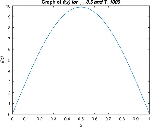For the numerical simulation, we take $\gamma =0.5$ and T=1000 (Figures 1 and 2).

Figure 1. For Example 6.1, the graph of $u(x,t)$ for $\gamma =0.5$ at t=0.5,0.75,5,900.

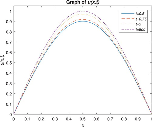
Figure 2. For Example 6.1, the graph of the source term $f\left(x\right)$, for $\gamma =0.5$.

Example 6.2

For particular example of IP-II, we consider $\alpha =2,f(x,t)=\frac{\mathrm{\Gamma }(3+\gamma )}{\mathrm{\Gamma }\left(3\right)}{t}^{-\gamma }\left(x^3-7x+6\frac{\sin \left(x\right)}{\sin \left(1\right)}\right)-6t\left(x-\frac{\sin \left(x\right)}{\sin \left(1\right)}\right)$ and $\phi \left(x\right)=0,E\left(t\right)=0.0278t^3.$ For the given data solution (23(23) $u(x,t)=\sum _{n=1}^{\mathrm{\infty }}\left\{{\phi }_n{E}_{\gamma ,1}\left({\lambda }_n{t}^{\gamma }\right)+a\left(t\right)f_n\left(t\right)\ast t^{\gamma -1}{E}_{\gamma ,\gamma }\left({\lambda }_n{t}^{\gamma }\right)\right\}{X}_n\left(x\right),$(23) ) can be written as $u(x,t)=\sum _{n=1}^{\mathrm{\infty }}\left\{a\left(t\right)f_n\left(t\right)\ast t^{\gamma -1}{E}_{\gamma ,\gamma }\left(n\pi t^{\gamma }\right)\right\}{X}_n\left(x\right),$ where $f_n\left(t\right)=⟨f(x,t),\sin \left(n\pi x\right)⟩.$

The expression for $a\left(t\right)$ is obtained as follows (by using (25(25) $a\left(t\right)={\left[{\int }_0^{1}f(x,t)\mathrm{d}x\right]}^{-1}\left[{}^c{D}_{0_{+},t}^{\gamma }E\left(t\right)-\mathcal{T}\left(t\right)-{\int }_0^{1}K(t,\tau )a\left(\tau \right)\mathrm{d}\tau \right].$(25) )): $a\left(t\right)={\left[{\int }_0^{1}f(x,t)\mathrm{d}x\right]}^{-1}\left[{}^c{D}_{0_{+},t}^{\gamma }\left(0.0278t^3\right)-{\int }_0^{t}K(t,\tau )a\left(\tau \right)\mathrm{d}\tau \right],$ where $K(t,\tau )=\sum _{n=1}^{\mathrm{\infty }}{f}_n\left(\tau \right)(t-\tau {)}^{\gamma -1}{E}_{\gamma ,\gamma }(n\pi (t-\tau {)}^{\gamma }).$ In this case, we are able to find the explicit expression for $a\left(t\right)$ as $a\left(t\right)=t^2,$ and the solution $u(x,t)$ becomes $u(x,t)=t^3\left(x^3-7x+6\frac{\sin \left(x\right)}{\sin \left(1\right)}\right)\sin \left(n\pi x\right).$ Let us mention that the eigenvalues of the spectral problem are not available explicitly. For particular examples in which the order of the space fractional derivative is some real number satisfying $1<\alpha <2$, an efficient numerical algorithm is needed.

7. Conclusions

For a space–time fractional differential equation, two inverse problems have been considered. The fractional derivatives involved in time and space are defined in Caputo's sense and are of order $0<\gamma <1$ and $1<\alpha <2$, respectively. From the over-specified condition, i.e. the given data at some time T, the inverse problem of recovering a space dependent source term has been considered (the inverse problem IP-I). A bi-orthogonal system of functions obtained from the spectral problem and its adjoint problem has been utilized to implement the generalized Fourier method. The series solution obtained is proved to be a regular solution of the inverse problem under certain assumptions on the given data (see Theorem 3.1) and the solution of the IP-I is proved to be stable. The determination of a time dependent source term from over-specified condition of integral type is the second inverse problem considered for the space–time fractional differential equation (the inverse problem IP-II). The result about the unique determination of a continuous source term is obtained by applying Banach fixed point theorem. The completeness of the set of eigenfunctions has been used to prove the uniqueness of $u(x,t)$. Some special cases of the inverse problems are discussed and particular numerical examples are provided. Let us mention that this analysis about the inverse problems can be extended to the problems involving the Hilfer fractional derivative [20]. Some other important inverse problems related to the space–time fractional differential equation (1(1) ${}^c{D}_{0_{+},t}^{\gamma }u(x,t)={}^c{D}_{0_{+},x}^{\alpha }u(x,t)+F(x,t),(x,t)\in \mathrm{\Pi },$(1) ) are worth to be considered. For example, the inverse problems of recovering the initial or boundary data and regularized algorithms for their reconstruction. Another interesting set of problems is related to the development of convergent numerical algorithms for solving direct and inverse problems related to Equation (1(1) ${}^c{D}_{0_{+},t}^{\gamma }u(x,t)={}^c{D}_{0_{+},x}^{\alpha }u(x,t)+F(x,t),(x,t)\in \mathrm{\Pi },$(1) ) with local or non-local boundary conditions.

Acknowledgements

The authors would like to express their gratitude to the anonymous reviewers for insightful comments which ultimately improve the quality of the paper.

Disclosure statement

No potential conflict of interest was reported by the authors.

References

- Slodička M. Determination of a solely time-dependent source in a semilinear parabolic problem by means of boundary measurements. J Comput Appl Math. 2015;289:433–440. doi: 10.1016/j.cam.2014.10.004
- Mohebbi A, Abbasi M. A fourth-order compact difference scheme for the parabolic inverse problem with an overspecification at a point. Inverse Probl Sci Eng. 2015;23:457–478. doi: 10.1080/17415977.2014.922075
- Aziz S, Malik SA. Identification of an unknown source term for a time fractional fourth order parabolic equation. Electron J Differ Equ. 2016;293:1–20.
- Sokolov IM, Klafter J. From diffusion to anomalous diffusion: a century after Einstein's Brownian motion. Chaos. 2005;15:026103. doi: 10.1063/1.1860472
- Fa KS. Fractal and generalized Fokker Planck equations: description of the characterization of anomalous diffusion in magnetic resonance imaging. J Stat Mech: Theor Exp. 2017;3:033207.
- Fedotov S, Korabel N. Subdiffusion in an external potential: anomalous effects hiding behind normal behavior. Phys Rev E. 2015;91:042112-1–042112-7.
- Kang PK, Dentz M, Le borgne T, et al. Anomalous transport in disordered fracture networks: spatial Markov model for dispersion with variable injection models. Adv Water Resour. 2017;106:80–94. doi: 10.1016/j.advwatres.2017.03.024
- Meerschaert MM, Sikorskii A. Stochastic models for fractional calculus. Berlin: De Gruyter; 2010.
- Chen ZQ, Kim P, Song R. Heat kernel estimates for the Dirichlet fractional Laplacian. J Eur Math Soc. 2010;12:1307–1329. doi: 10.4171/JEMS/231
- Salari L, Rondoni L, Giberti C, et al. A simple non-chaotic map generating subdiffusive, diffusive and superdiffusive dynamics. Chaos. 2015;25:073113. doi: 10.1063/1.4926621
- Weiss GH. Aspects and applications of the random walk. Amsterdam: North-Holland; 1994.
- Hughes DB. Random walks and random environments. Vol. I, Random walks. Oxford: Clarendon Press; 1995.
- Mura A, Pagnini G. Characterization and simulations of a class of stochastic processes to model anomalous diffusion. J Phys A: Math Theor. 2008;41:285003. doi: 10.1088/1751-8113/41/28/285003
- Metzler R, Jeon JH, Cherstvy AG, et al. Anomalous diffusion models and their properties: non-stationarity, non-ergodicity, and ageing at the centenary of single particle tracking. Phys Chem Chem Phys. 2014;16:24128–24164. doi: 10.1039/C4CP03465A
- Klages R, Radons G, Sokolov IM. Anomalous transport. Weinheim: WILEY-VCH Verlag GmbH & Co. KGaA; 2008.
- Sierociuk D, Skovranek T, Macias M, et al. Diffusion process modeling by using fractional-order models. Appl Math Comput. 2015;257:2–11.
- Povstenko Y. Linear fractional diffusion-wave equation for scientists and engineers. Switzerland: Springer International Publishing; 2015.
- Ionescu C, Lopes A, Copot D, et al. The role of fractional calculus in modelling biological phenomena: a review. Commun Nonlinear Sci Numer Simul. 2017;51:141–159. doi: 10.1016/j.cnsns.2017.04.001
- Höfling F, Franosch T. Anomalous transport in the crowded world of biological cells. Rep Prog Phys. 2013;76:046602 (50pp). doi: 10.1088/0034-4885/76/4/046602
- Hilfer R. Applications of fractional calculus in physics. Singapore: World Scientific; 2000.
- Tarasov VE. Fractional dynamics: applications of fractional calculus to dynamics of particles, fields and media. Beijing: Springer-Verlag; 2010.
- Machado JAT, Lopes AM. Relative fractional dynamics of stock markets. Nonlinear Dyn. 2016;86:1613–1619. doi: 10.1007/s11071-016-2980-1
- Bagley RL, Torvik PJ. A theoretical basis for the application of fractional calculus to viscoelasticity. J Rheol. 1983;27:201–210. doi: 10.1122/1.549724
- Mainardi F. Fractional calculus and waves in linear viscoelasticity. London: Imperial College Press; 2010.
- Caputo M, Carcione JM, Botelho MAB. Modeling extreme-event precursors with the fractional diffusion equation. Fract Calc Appl Anal. 2015;18:208–222. doi: 10.1515/fca-2015-0014
- Kirane M, Malik SA. Determination of an unknown source term and the temperature distribution for the linear heat equation involving fractional derivative in time. Appl Math Comput. 2011;218:163–170.
- Kirane M, Malik SA, Al-Gwaiz MA. An inverse source problem for a two dimensional time fractional diffusion equation with nonlocal boundary conditions. Math Methods Appl Sci. 2013;36:1056–1069. doi: 10.1002/mma.2661
- Ali M, Malik SA. An inverse problem for a family of time fractional diffusion equations. Inverse Probl Sci Eng. 2017;25:1299–1322. doi: 10.1080/17415977.2016.1255738
- Furati KM, Iyiola OS, Kirane M. An inverse problem for a generalised fractional diffusion. Appl Math Comput. 2014;249:24–31.
- Wei T, Sun L, Li Y. Uniqueness for an inverse space-dependent source term in a multi-dimensional time-fractional diffusion equation. Appl Math Lett. 2016;61:108–113. doi: 10.1016/j.aml.2016.05.004
- Malik SA, Aziz S. An inverse source problem for a two parameter anomalous diffusion equation with nonlocal boundary conditions. Comput Math Appl. 2017;73:2548–2560. doi: 10.1016/j.camwa.2017.03.019
- Lopushanska H, Rapita V. Inverse coefficient problem for the semi-linear fractional telegraph equation. Electron J Differ Equ. 2015;153:1–13.
- Šišková K, Slodička M. Recognition of a time-dependent source in a time-fractional wave equation. Appl Numer Math. 2017;121:1–17. doi: 10.1016/j.apnum.2017.06.005
- Aziz S, Malik SA. Identification of an unknown source term for a time fractional fourth-order parabolic equation. Electron J Differ Equ. 2016;293:1–28.
- Tatar S, Ulusoy S. An inverse source problem for a one dimensional space–time fractional diffusion equation. Appl Anal. 2015;94:2233–2244. doi: 10.1080/00036811.2014.979808
- Feng P, Karimov ET. Inverse source problems for time-fractional mixed parabolic-hyperbolic-type equations. J Inverse Ill-Posed Probl. 2015;23:339–353. doi: 10.1515/jiip-2014-0022
- Liu CS, Chen W, Fu Z. A multiple-scale MQ-RBF for solving the inverse Cauchy problems in arbitrary plane domain. Eng Anal Bound Elem. 2016;68:11–16. doi: 10.1016/j.enganabound.2016.02.011
- Al-Jamal MF. A backward problem for the time-fractional diffusion equation. Math Methods Appl Sci. 2017;40:2466–2474. doi: 10.1002/mma.4151
- Tuan NH, Long LD, Nguyen VT, et al. On a final value problem for the time-fractional diffusion equation with inhomogeneous source. Inverse Probl Sci Eng. 2017;25:1367–1395. doi: 10.1080/17415977.2016.1259316
- Lukashchuk SY. Estimation of parameters in fractional subdiffusion equations by the time integral characteristics method. Comput Math Appl. 2011;62:834–844. doi: 10.1016/j.camwa.2011.03.058
- Janno J. Determination of the order of fractional derivative and a kernel in an inverse problem for a generalized time fractional diffusion equation. Electron J Differ Equ. 2016;199:1–28.
- Chen S, Jiang XY. Parameter estimation for a new anomalous thermal diffusion model in layered media. Comput Math Appl. 2017;73:1172–1181. doi: 10.1016/j.camwa.2016.10.008
- Li Z, Imanuvilov OY, Yamamoto M. Uniqueness in inverse boundary value problems for fractional diffusion equations. Inverse Probl. 2015;32:015004.
- Li Z, Yamamoto M. Uniqueness for inverse problems of determining orders of multi-term time-fractional derivatives of diffusion equation. Appl Anal. 2015;94:570–579. doi: 10.1080/00036811.2014.926335
- Jiang D, Li Z, Liu Y, et al. Weak unique continuation property and a related inverse source problem for time-fractional diffusion–advection equations. Inverse Probl. 2017;33:055013.
- Liu Y, Rundell W, Yamamoto M. Strong maximum principle for fractional diffusion equations and an application to an inverse source problem. Fract Calc Appl Anal. 2016;19:888–906.
- Tatar S, Tinaztepe R, Ulusoy S. Simultaneous inversion for the exponents of the fractional time and space derivatives in the space–time fractional diffusion equation. Appl Anal. 2016;95:1–23. doi: 10.1080/00036811.2014.984291
- Jia J, Peng J, Yang J. Harnack's inequality for a space–time fractional diffusion equation and application to an inverse source problem. J Differ Equ. 2017;262:4415–4450. doi: 10.1016/j.jde.2017.01.002
- Ali M, Aziz S, Malik SA. Inverse problem for a space–time fractional diffusion equation: application of fractional Sturm–Liouville operator. Math Methods Appl Sci. 2018;41:2733–2744. doi: 10.1002/mma.4776
- Ali M, Aziz S, Malik SA. Inverse source problem for a space–time fractional diffusion equation. Fract Calc Appl Anal. 2018;21:844–863. doi: 10.1515/fca-2018-0045
- Gara R, Gorenflo R, Polito F, et al. Hilfer–Prabhakar derivatives and some applications. Appl Math Comput. 2014;242:576–589.
- Gorenflo R, Kilbas AA, Mainardi F Mittag–Leffler functions, related topics and applications. Berlin: Springer-Verlag; 2014.
- Podlubny I. Fractional differential equations. San Diego (CA): Academic Press; 1999.
- Samko SG, Kilbas AA, Marichev DI. Fractional integrals and derivatives: theory and applications. Amsterdam: Gordon and Breach Science Publishers; 1993.
- Aleroev TS, Kirane M, Tang YF. The boundary-value problem for a differential operator of fractional order. J Math Sci. 2013;194:499–512. doi: 10.1007/s10958-013-1543-y