The two-step method for determining a piecewise-continuous refractive index of a 2D scatterer by near field measurements

Abstract

The problem of determining an unknown piecewise-continuous refractive index of an inhomogeneous scatterer is considered. The boundary value problem is reduced to the Lippmann–Schwinger integral equation. The solution of the inverse problem is obtained in two steps. At the first step, the integral equation of the first kind is solved in the inhomogeneity region using measured values of the total field outside the region. It is proved that the solution to the integral equation of the first kind is unique in the class of piecewise constant functions. At the second step, the unknown refractive index is explicitly calculated via the found solution of the integral equation and the given total field. The proposed method was implemented and verified by solving a test inverse problem with a given refractive index. Efficiency of the two-step method was approved by comparison between the exact solution and the approximate ones.

Keywords:

• Refractive index reconstruction
• integral equations
• solution uniqueness
• inverse problems
• near field data

1. Introduction

The present paper describes a novel two-step method (TSM) for solving a two-dimensional inverse problem of recovering the refractive index of an inhomogeneous lossy scatterer.

Formulations of inverse problems in the two-dimensional space ${\mathbb{R}}^2$ have been considered through several decades (see, e.g. [1,2] and the bibliography therein) and are relevant up to now [3–5].

One of the approaches to solving such problems involves minimizing some error functionals. Such methods include Tikhonov regularization of the minimized functionals as well as iterative procedures that require a good initial approximation [6].

In [7] there was proposed a novel iterative technique that converges globally, i.e. it does not require a good initial approximation. Papers [8–10] represent more advanced globally convergent algorithms (the so-called convexification approach) for coefficient inverse problems. This approach based on the construction of a weighted globally strictly convex cost functional eliminates the phenomenon of multiple local minima of least-squares cost functionals and provides the global convergence to the correct solution of the gradient projection method.

We propose a non-iterative approach for identifying an unknown function $n\left(x\right)$ represents the contrast source of an inhomogeneous scatterer of a monochromatic wave. This approach was first used in [11] and was named the TSM for solving inverse problems of recovering an unknown refractive index (the method is also described in [12]).

The paper is organized as follows.

In Section 2, we consider the direct problem of diffraction by an inhomogeneous obstacle characterized by a piecewise-continuous refractive index. The original boundary value problem (BVP) for the Helmholtz equation is given in the quasiclassical formulation [13] which differs from the one considered in [14] and is seemingly more relevant from the physical point of view.

Since TSM is based on the contrast source integral representations, it is important to prove the equivalency between the original BVP and used system of integral equations (IEs). This system is shown to be an equivalent formulation of the diffraction problem and includes the Lippmann–Schwinger equation (LSE) which follows from the BVP. We prove theorems on the smoothness of solutions to the LSE and establish its unique solvability. This study is given in Section 2.2.

In the next section, the statement of the inverse problem is given, and the TSM for its solving is described. The method consists in solving a linear IE of the first kind (step 1) with respect to the current $J\left(x\right)=\left(k^2\right(x)-k_0^2)u\left(x\right)$ (here $u\left(x\right)$ is the total field, $k_0$ is the given wave number of free space), followed by an explicit calculation of the sought-for refractive index k (step 2).

The IEs used in TSM are well known under the name of source-type IEs (see, e.g. [15,16] and the bibliography therein). However, we use another approach for their studying. In this work, the linear IE of the first kind is solved with subsequent explicit calculation of the unknown function $k\left(x\right),$ whereas in [15] authors use an error functional minimization technique.

Solving the used IE is known to be an ill-posed problem since the uniqueness of a solution is not guaranteed; we show that the corresponding homogeneous IE has an infinite set of smooth solutions. However, it can be proved that the solution to the IE is unique in the class of piecewise constant functions. The sufficient conditions for the IE unique solvability are represented in Section 3.2.

Such a choice of the solution space is seemingly valid for several reasons. First, we use piecewise constants for the approximation of the function $J\left(x\right)$ rather than for studying discontinuous currents. Further, the total field u corresponding to the piecewise constant J satisfies the smoothness conditions which are formulated in the direct problem. That is due to the representation of the field u via the potential with the density J. Finally, application of piecewise constant functions with rectangular support is a relevant approach for solving some practical problems, e.g. diffraction by nanomaterials which have a periodic structure with a rectangular grid. In such problems, the grid is given, whereas the values of an unknown function (e.g. permittivity) are to be found.

In TSM, we define (and fixate) the computational grid. Therefore, classical theorems on the convergence of the method are not considered in the article. Such an approach is valid in practice since it is usually clear what accuracy (and, consequently, what grid) is needed. For example, it is sufficient to consider grids with 2 to 5 mm step in the method of microwave tomography for the breast cancer early diagnosis (thus, any grid refinement is no use).

The last section of the paper is concerned with numerical experiments whose results are represented in Figures 1–6. The modelling of the inverse scattering problem is organized as follows. At the beginning, we define the wave number $k_0$ of the space and the function $n\left(x\right)$ which represents the space-dependent contrast of the scattering object. Then we solve the direct problem of diffraction of a given field $u_0\left(x\right)$ with respect to the total field $u\left(x\right).$ In all experiments, we consider the incident field $u_0$ of a point source located outside the scatterer. Thus, we obtain the synthetic field data. Further, the TSM is applied for solving the model inverse problem. At the first step, we use the contrast source integral representation outside the scatterer and numerically solve the IE of the first kind to find the current J, being the product of the contrast of the scattering object and the total field. At the second step we explicitly calculate the sought-for function $k\left(x\right)$ using the LSE.

Figure 1. The given function $k\left(x\right).$

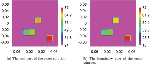
Figure 2. The approximate solution of the inverse problem with noiseless data.

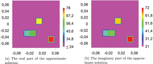
Figure 3. The approximate solution of the inverse problem with noisy data. The noise level is denoted by $\mathbf{n}\mathbf{l}.$

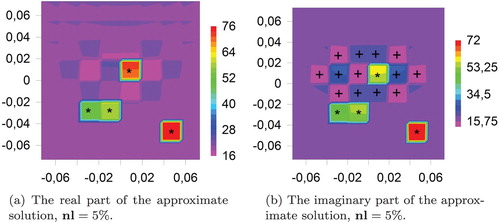
Figure 4. Solutions' real part obtained before the data processing at various noise levels (denoted by $\mathbf{n}\mathbf{l}$).

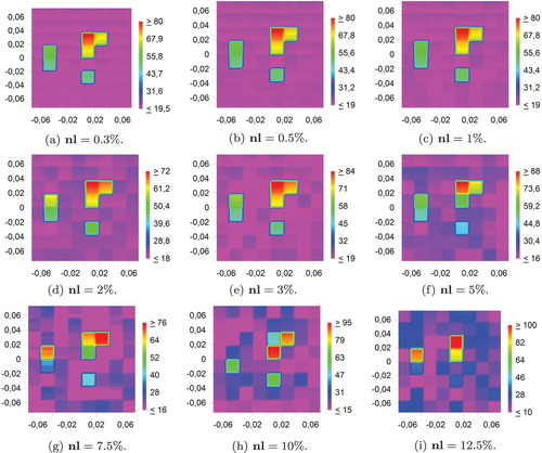
Figure 5. Real part of two solutions used for postprocessing: the data is noisy, $\mathbf{n}\mathbf{l}=5\mathrm{\%}.$ True inhomogeneities and artefacts are marked by * and +, respectively.

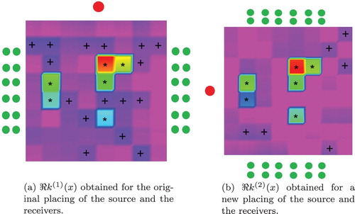
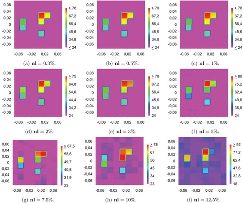
Figure 6. Solutions' real part obtained after pre- and postprocessing at various noise levels (denoted by $\mathbf{n}\mathbf{l}$).

Section 4 also contains comments on the implementation of the numerical method for solving the inverse problem, as well as a detailed description of our technique of solutions' refinement. The refinement is made in two steps. First, we propose to filter the noise of near field data. Second, we propose a postprocessing procedure for finding true inhomogeneities in a more accurate way, as well as for excluding artefacts and levelling of the background. The numerical simulation shows high efficiency of the proposed methods if the noise is less than 5% of the pure data.

2. Direct problem of diffraction

We consider the problem of diffraction in the two-dimensional unbounded space ${\mathbb{R}}^2$ filled with isotropic medium. The homogeneous space is characterized by a given wave number $k_0=\omega /c>0,$ where $\omega >0$ and c>0 are, respectively, the frequency and the speed of the incident wave $U_0(x,t)=u_0\left(x\right)e^{-\mathrm{i}\omega t}.$

2.1. Statement of the direct problem of diffraction

We consider the problem of diffraction of a monochromatic wave by a rectangular scatterer P, $P=\left\{x=(x_1,x_2):a_1<x_1<b_1,a_2<x_2<b_2\right\}.$ We introduce the mesh of nodes $x_{1,i_1}=a_1+\left(b_1-a_1/n\right)i_1,x_{2,i_2}=a_2+\left(b_2-a_2/n\right)i_2,$ and the set of finite elements ${\mathrm{\Pi }}_{i_1{i}_2}=\left\{x:x_{k,i_k}<x_k<x_{k,i_k+1}\right\},$  k=1,2 and $0\le i_k\le n-1.$

We denote the unions of vertices and sides of the rectangles ${\mathrm{\Pi }}_I$ by $V_P$ and $S_P,$ respectively, and introduce the notation $\mathrm{\partial }{\mathrm{\Pi }}_I^{\prime }={\mathrm{\Pi }}_I\setminus V_P,\mathrm{\partial }{P}^{\prime }=P\setminus V_P,P^{″}=P\setminus S_P.$ Define piecewise constant functions in the region P, (1) ${\chi }_{i_1{i}_2}\left(x\right)=\left\{\begin{array}{ll}1,& x\in {\mathrm{\Pi }}_{i_1{i}_2},\\ 0,& x\notin {\mathrm{\Pi }}_{i_1{i}_2},\end{array}\right.$(1) and assume that P is an inhomogeneous domain characterized by a piecewise Hölder function $k\left(x\right).$ More precisely, $k\left(x\right)=n\left(x\right)k_0=k_{i_1{i}_2}\left(x\right)$ at $x\in {\mathrm{\Pi }}_{i_1{i}_2},$ and $k_{i_1{i}_2}\left(x\right)$ are Hölder continuous functions in ${\mathrm{\Pi }}_{i_1{i}_2},$ $k_{i_1{i}_2}\in C^{0,\alpha }\left({\mathrm{\Pi }}_{i_1{i}_2}\right),$ where $\alpha \in (0,1).$

Remark 2.1

According to the above assumptions, the unknown $k\left(x\right)$ (or $n\left(x\right)$) can be a discontinuous function that has jumps on $\mathrm{\partial }{\mathrm{\Pi }}_I$ or a continuous function. Thus, one can also consider a function $k\left(x\right)\in C^{0,\alpha }\left(P\right).$

Introduce the multi-index $I=\left(i_1{i}_2\right)$ and define the function $k\left(x\right)$ for each $x\in P^{″}$ by equality $k\left(x\right)=\sum _I{k}_I\left(x\right){\chi }_I\left(x\right).$ At points $x\in S_p$ the function $k\left(x\right)$ can be defined via the one-sided limit from any side of the line $\mathrm{\partial }{\mathrm{\Pi }}_{i_1{i}_2}.$

We represent the total field $U(x;t)$ via the sum $U(x;t)=U_0(x;t)+U_s(x;t),$ where $U_s=u_s\left(x\right)e^{-\mathrm{i}\omega t}$ is the scattered field. Since the fields depend on time harmonically, then it suffices to formulate the scattering problem for the scalar complex amplitude $u\left(x\right)=u_0\left(x\right)+u_s\left(x\right)$ of the total field.

We define the incident wave as follows: (2) $u_0\left(x\right)=\frac{i}{4}{H}_0^{\left(1\right)}(k_0|x-x_0|).$(2)

Here $H_0^{\left(1\right)}$ is the Hankel function of the first kind [17], and $x_0$ is a fixed point outside $\overline{P}.$ The field $u_0$ is a solution to equation $(\mathrm{△}+k_0^2)u_0\left(x\right)=-\delta (x-x_0)$ satisfying the Sommerfeld radiation conditions $u_0=O\left(r^{-1/2}\right),\frac{\mathrm{\partial }{u}_0}{\mathrm{\partial }r}-i{k}_0{u}_0=o\left(r^{-1/2}\right),r=|x|\to \mathrm{\infty }.$ The direct problem of diffraction is to find a function $u\left(x\right),$ (3) $u\in C^1({\mathbb{R}}^2\setminus \{x_0\left\}\right)\bigcap _I{C}^2\left({\mathrm{\Pi }}_I\right)\bigcap C^{\mathrm{\infty }}({\mathbb{R}}^2\setminus (\overline{P}\cup \left\{x_0\right\}\left)\right),$(3) which satisfies the Helmholtz equation (4) $(\mathrm{△}+k_I^2(x\left)\right)u\left(x\right)=0,x\in {\mathrm{\Pi }}_I;(\mathrm{△}+k_0^2)u\left(x\right)=-\delta (x-x_0),x,x_0\in {\mathbb{R}}^2\setminus \left(\overline{P}\right),$(4) as well as the transmission conditions (5) ${\left.\left[u\right]\right|}_{\mathrm{\partial }{\mathrm{\Pi }}_I}=0,{\left.\left[\frac{\mathrm{\partial }u}{\mathrm{\partial }\mathbf{n}}\right]\right|}_{\mathrm{\partial }{\mathrm{\Pi }}_I^{\prime }}=0,$(5) the energy finiteness condition (6) $u\in H_{loc}^1({\mathbb{R}}^2\setminus \{x_0\left\}\right),$(6) and the Sommerfeld radiation conditions (7) $u=O\left(r^{-1/2}\right),\frac{\mathrm{\partial }u}{\mathrm{\partial }r}-i{k}_{0}u=o\left(r^{-1/2}\right),r=|x|\to \mathrm{\infty }.$(7)

Any solution of problem (4(4) $(\mathrm{△}+k_I^2(x\left)\right)u\left(x\right)=0,x\in {\mathrm{\Pi }}_I;(\mathrm{△}+k_0^2)u\left(x\right)=-\delta (x-x_0),x,x_0\in {\mathbb{R}}^2\setminus \left(\overline{P}\right),$(4) )–(7(7) $u=O\left(r^{-1/2}\right),\frac{\mathrm{\partial }u}{\mathrm{\partial }r}-i{k}_{0}u=o\left(r^{-1/2}\right),r=|x|\to \mathrm{\infty }.$(7) ) satisfying continuity conditions (3(3) $u\in C^1({\mathbb{R}}^2\setminus \{x_0\left\}\right)\bigcap _I{C}^2\left({\mathrm{\Pi }}_I\right)\bigcap C^{\mathrm{\infty }}({\mathbb{R}}^2\setminus (\overline{P}\cup \left\{x_0\right\}\left)\right),$(3) ) is called a quasiclassical solution to the direct scattering problem in differential statement $\left({\mathcal{P}}_1\right).$

Let us prove the uniqueness of a solution to the problem $\left({\mathcal{P}}_1\right).$

Theorem 2.1

For any wave number $k_0>0$ and any function $k\left(x\right)$ such that $\mathrm{\Re }k\left(x\right)>0,$ $\mathrm{\Im }k\left(x\right)\ge 0$ the problem $\left({\mathcal{P}}_1\right)$ has at most one quasiclassical solution.

Proof.

Since $\left({\mathcal{P}}_1\right)$ is a linear boundary value problem, it is sufficient to show that the homogeneous problem with $u_0\equiv 0$ in ${\mathbb{R}}^2$ has only the trivial solution $u_s\equiv u\equiv 0.$

1. Let B be a sufficiently large circle of radius R such that $\overline{P}\subset B.$ Define the bounded domain $Q:=B\setminus \left(\overline{P}\right)$ with the boundary $\mathrm{\partial }V=\mathrm{\partial }B\cup \mathrm{\partial }P$ and the unbounded region $W:={\mathbb{R}}^2\setminus \overline{B}.$

The boundary value problem for u can be reduced to a transmission problem in the subdomains ${\mathrm{\Pi }}_I,$ Q and W. The problem is to find the function $u\left(x\right)$ which satisfies the Helmholtz equations, (8) $\begin{array}{rl}(\mathrm{\Delta }+k_0^2)u\left(x\right)& =0,x\in Q\cup W,\\ (\mathrm{\Delta }+k_I^2(x\left)\right)u\left(x\right)& =0,x\in {\mathrm{\Pi }}_I,\end{array}$(8) as well as transmission conditions (9) $\begin{array}{rl}\left[u\right(x\left)\right]& =0,x\in \mathrm{\partial }{\mathrm{\Pi }}_I\cup \mathrm{\partial }P\cup \mathrm{\partial }B,\\ \left[\frac{\mathrm{\partial }u\left(x\right)}{\mathrm{\partial }\mathbf{n}}\right]& =0,x\in \mathrm{\partial }{\mathrm{\Pi }}_I^{\prime }\cup \mathrm{\partial }{P}^{\prime }\cup \mathrm{\partial }B.\end{array}$(9) The function u also satisfies radiation conditions (7(7) $u=O\left(r^{-1/2}\right),\frac{\mathrm{\partial }u}{\mathrm{\partial }r}-i{k}_{0}u=o\left(r^{-1/2}\right),r=|x|\to \mathrm{\infty }.$(7) ).

Let us apply the first Green formula ${\int }_Q(v\mathrm{△}u+\mathrm{\nabla }u\cdot \mathrm{\nabla }v)dx={\int }_{\mathrm{\partial }V}v\left(\mathrm{\partial }u/\mathrm{\partial }\mathbf{n}\right)\mathrm{d}s$ to the functions u and $v=\overline{u}$ in the bounded domains ${\mathrm{\Pi }}_I\subset P$ and Q. Taking into account the Helmholtz equations, we derive (10a) ${\int }_{{\mathrm{\Pi }}_I}(\overline{u}\mathrm{△}u+|\mathrm{\nabla }u{|}^2)\mathrm{d}x=-{\int }_{{\mathrm{\Pi }}_I}{k}_I^2|u{|}^2\mathrm{d}x+{\int }_{{\mathrm{\Pi }}_I}|\mathrm{\nabla }u{|}^2\mathrm{d}x={\int }_{\mathrm{\partial }{\mathrm{\Pi }}_I^{\prime }}\overline{u}\frac{\mathrm{\partial }u}{\mathrm{\partial }\mathbf{n}}\mathrm{d}s,$(10a) (10b) ${\int }_Q(\overline{u}\mathrm{△}u+|\mathrm{\nabla }u{|}^2)\mathrm{d}x=-k_0^2{\int }_Q|u{|}^2\mathrm{d}x+{\int }_Q|\mathrm{\nabla }u{|}^2\mathrm{d}x={\int }_{\mathrm{\partial }{Q}^{\prime }}\overline{u}\frac{\mathrm{\partial }u}{\mathrm{\partial }\mathbf{n}}\mathrm{d}s.$(10b)

Summing up Equations (10a(10a) ${\int }_{{\mathrm{\Pi }}_I}(\overline{u}\mathrm{△}u+|\mathrm{\nabla }u{|}^2)\mathrm{d}x=-{\int }_{{\mathrm{\Pi }}_I}{k}_I^2|u{|}^2\mathrm{d}x+{\int }_{{\mathrm{\Pi }}_I}|\mathrm{\nabla }u{|}^2\mathrm{d}x={\int }_{\mathrm{\partial }{\mathrm{\Pi }}_I^{\prime }}\overline{u}\frac{\mathrm{\partial }u}{\mathrm{\partial }\mathbf{n}}\mathrm{d}s,$(10a) ) and (10b(10b) ${\int }_Q(\overline{u}\mathrm{△}u+|\mathrm{\nabla }u{|}^2)\mathrm{d}x=-k_0^2{\int }_Q|u{|}^2\mathrm{d}x+{\int }_Q|\mathrm{\nabla }u{|}^2\mathrm{d}x={\int }_{\mathrm{\partial }{Q}^{\prime }}\overline{u}\frac{\mathrm{\partial }u}{\mathrm{\partial }\mathbf{n}}\mathrm{d}s.$(10b) ) and using the transmission conditions (9(9) $\begin{array}{rl}\left[u\right(x\left)\right]& =0,x\in \mathrm{\partial }{\mathrm{\Pi }}_I\cup \mathrm{\partial }P\cup \mathrm{\partial }B,\\ \left[\frac{\mathrm{\partial }u\left(x\right)}{\mathrm{\partial }\mathbf{n}}\right]& =0,x\in \mathrm{\partial }{\mathrm{\Pi }}_I^{\prime }\cup \mathrm{\partial }{P}^{\prime }\cup \mathrm{\partial }B.\end{array}$(9) ), we obtain (11) $\begin{array}{rl}{\int }_{\mathrm{\partial }B}\overline{u}\frac{\mathrm{\partial }u}{\mathrm{\partial }\mathbf{n}}\mathrm{d}s& =-\sum _I{\int }_{{\mathrm{\Pi }}_I}{k}_I^2|u{|}^2\mathrm{d}x-k_0^2{\int }_Q|u{|}^2\mathrm{d}x\\ & +{\int }_Q|\mathrm{\nabla }u{|}^2\mathrm{d}x+\sum _I{\int }_{{\mathrm{\Pi }}_I}|\mathrm{\nabla }u{|}^2\mathrm{d}x=-{\int }_{\mathrm{\partial }B}\overline{u}\frac{\mathrm{\partial }u}{\mathrm{\partial }\mathbf{n}}\mathrm{d}s.\end{array}$(11)

Remark 2.2

If $u\left(x\right)$ belongs to appropriate Sobolev classes [18], the Green formulas can be applied in the entire region P, and the above evaluation can be written in a shorter form.

2. Taking into account conditions (7(7) $u=O\left(r^{-1/2}\right),\frac{\mathrm{\partial }u}{\mathrm{\partial }r}-i{k}_{0}u=o\left(r^{-1/2}\right),r=|x|\to \mathrm{\infty }.$(7) ), we get $\begin{array}{rl}\mathrm{\Im }\left({\int }_{\mathrm{\partial }B}\overline{u}\frac{\mathrm{\partial }u}{\mathrm{\partial }\mathbf{n}}\mathrm{d}s\right)& =\mathrm{\Im }\left({\int }_{\mathrm{\partial }B}(i{k}_{0}u+o(R^{-1/2}\left)\right)\overline{u}\mathrm{d}s\right)\\ & =k_0{\int }_{\mathrm{\partial }B}|u{|}^2\mathrm{d}s+{\int }_{\mathrm{\partial }B}o\left(R^{-1}\right)\mathrm{d}s=k_0{\int }_{\mathrm{\partial }B}|u{|}^2\mathrm{d}s+o\left(1\right)=0.\end{array}$ By virtue of the Rellich lemma (see [2, p.55]) we deduce $u\equiv 0$ in W, which implies that the solution of the problem is trivial outside the inhomogeneity domain P.

3. Let us prove that $u\equiv 0$ in P.

Introduce the function $G(x,y)=\frac{i}{4}{H}_0^{\left(1\right)}(k_0|x-y|).$ Consider an arbitrary rectangle ${\overline{\mathrm{\Pi }}}_I$ such that $\mathrm{\partial }{\mathrm{\Pi }}_I\cap \mathrm{\partial }P=\mathrm{\partial }{\mathrm{\Pi }}_I\cap \mathrm{\partial }({\mathbb{R}}^2\setminus P)=S\ne \varnothing$). We will use the integral representation of the solution u, (12) $\begin{array}{rl}u\left(x\right)& ={\int }_{P}G(x,y)\left(k^2\right(y)-k_0^2)u\left(y\right)\mathrm{d}y\\ & =\sum _{J\ne I}{\int }_{{\mathrm{\Pi }}_J}G(x,y)\left(k_J^2\right(y)-k_0^2)u\left(y\right)\mathrm{d}y+{\int }_{{\mathrm{\Pi }}_I}G(x,y)\left(k_I^2\right(y)-k_0^2)u\left(y\right)\mathrm{d}y\\ & =v\left(x\right)+w\left(x\right),x\in {\overline{\mathrm{\Pi }}}_I.\end{array}$(12) Let us investigate $u\left(x\right)$ in a sufficiently small vicinity U of an arbitrary point $x_0\in S\setminus \mathrm{\partial }S.$ Since the kernels of the integral operators are infinitely differentiable for any $J\ne I,$ then $v\left(x\right)\in C^{\mathrm{\infty }}\left(U\right).$ Using continuity conditions (3(3) $u\in C^1({\mathbb{R}}^2\setminus \{x_0\left\}\right)\bigcap _I{C}^2\left({\mathrm{\Pi }}_I\right)\bigcap C^{\mathrm{\infty }}({\mathbb{R}}^2\setminus (\overline{P}\cup \left\{x_0\right\}\left)\right),$(3) ) and representation (12(12) $\begin{array}{rl}u\left(x\right)& ={\int }_{P}G(x,y)\left(k^2\right(y)-k_0^2)u\left(y\right)\mathrm{d}y\\ & =\sum _{J\ne I}{\int }_{{\mathrm{\Pi }}_J}G(x,y)\left(k_J^2\right(y)-k_0^2)u\left(y\right)\mathrm{d}y+{\int }_{{\mathrm{\Pi }}_I}G(x,y)\left(k_I^2\right(y)-k_0^2)u\left(y\right)\mathrm{d}y\\ & =v\left(x\right)+w\left(x\right),x\in {\overline{\mathrm{\Pi }}}_I.\end{array}$(12) ), we obtain (13) $w\left(x\right)\in C^2(U\setminus S)\cap C^1\left(U\right)\cap H^2\left(U\right).$(13) The function $w\left(x\right)$ satisfies equation $(\mathrm{△}+k_I^2(x\left)\right)w\left(x\right)=0$ in the subdomain $U\cap {\mathrm{\Pi }}_I$ with a coefficient $k_I^2\left(x\right)\in C^{\alpha }(\overline{U}\cap {\mathrm{\Pi }}_I).$ Hence (see §12 Ch. III in [19]) the inclusion $w\left(x\right)\in C^{2,\alpha }(\overline{U}\cap {\mathrm{\Pi }}_I)$ holds. Since the boundary values of the function $w\left(x\right)$ on S are smooth, $w{|}_S=u{|}_S-v{|}_S=-v{|}_S\in C^{\mathrm{\infty }}\left(S\right),$ then $w\left(x\right)\in C^{2,\alpha }\left(U\right).$

Thus, the function $u\in C^2\left(U\right)$ satisfies the Helmholtz equation $(\mathrm{△}+k^2(x\left)\right)u\left(x\right)=0$ with a piecewise Hölder coefficient in U. Consequently, $u\equiv 0$ in U. By virtue of the unique continuation principle ([14, p.272]) it follows from $u\equiv 0$ in $U\cap {\mathrm{\Pi }}_I$ that $u\equiv 0$ in the entire rectangle ${\mathrm{\Pi }}_I.$ Similar to the above reasoning, we can conclude that $u\equiv 0$ everywhere in P.

2.2. The LSE: smoothness of a solution

Let us derive the boundary value problem (4(4) $(\mathrm{△}+k_I^2(x\left)\right)u\left(x\right)=0,x\in {\mathrm{\Pi }}_I;(\mathrm{△}+k_0^2)u\left(x\right)=-\delta (x-x_0),x,x_0\in {\mathbb{R}}^2\setminus \left(\overline{P}\right),$(4) )–(7(7) $u=O\left(r^{-1/2}\right),\frac{\mathrm{\partial }u}{\mathrm{\partial }r}-i{k}_{0}u=o\left(r^{-1/2}\right),r=|x|\to \mathrm{\infty }.$(7) ) to a system of IEs. Rewrite the Helmholtz equation in the domains ${\mathrm{\Pi }}_I$ as follows: (14) $\mathrm{\Delta }u\left(x\right)+k_0^{2}u\left(x\right)=(k_0^2-k_I^2(x\left)\right)u\left(x\right),x\in {\mathrm{\Pi }}_I.$(14) In the bounded domain ${\mathrm{\Pi }}_0=B\setminus \overline{P},$ we have (15) $\mathrm{\Delta }u\left(x\right)+k_0^{2}u\left(x\right)=-\delta (x-x_0),x\in {\mathrm{\Pi }}_0,$(15) where $B\supset P$ is a circle of sufficiently large radius and $\mathrm{\partial }B=S.$

By the second Green formula, we derive (16) $\begin{array}{rl}{\int }_{\mathrm{\partial }{\mathrm{\Pi }}_I^{\prime }}\left(\frac{\mathrm{\partial }u\left(y\right)}{\mathrm{\partial }\mathbf{n}}G(x,y)-\frac{\mathrm{\partial }G(x,y)}{\mathrm{\partial }\mathbf{n}}u\left(y\right)\right)\mathrm{d}{s}_y& ={\int }_{{\mathrm{\Pi }}_I}(\mathrm{\Delta }u\left(y\right)G(x,y)-\mathrm{\Delta }G(x,y)u\left(y\right))\mathrm{d}y\\ & ={\int }_{{\mathrm{\Pi }}_I}(-k_I^2\left(y\right)u\left(y\right)G(x,y)+k_0^{2}G(x,y)u\left(y\right)\\ & +\delta (x-y)u\left(y\right))\mathrm{d}y\\ & =u\left(x\right)-{\int }_{{\mathrm{\Pi }}_I}\left(k_I^2\right(y)-k_0^2)G(x,y)u\left(y\right)\mathrm{d}y,\\ & \times x\in {\mathrm{\Pi }}_I,\end{array}$(16) (17) $\begin{array}{rl}{\int }_{\mathrm{\partial }{\mathrm{\Pi }}_J^{\prime }}\left(\frac{\mathrm{\partial }u\left(y\right)}{\mathrm{\partial }\mathbf{n}}G(x,y)-\frac{\mathrm{\partial }G(x,y)}{\mathrm{\partial }\mathbf{n}}u\left(y\right)\right)\mathrm{d}{s}_y& ={\int }_{{\mathrm{\Pi }}_J}(\mathrm{\Delta }u\left(y\right)G(x,y)-\mathrm{\Delta }G(x,y)u\left(y\right))\mathrm{d}y\\ & ={\int }_{{\mathrm{\Pi }}_J}(-k_J^2\left(y\right)u\left(y\right)G(x,y)+k_0^{2}G(x,y)u\left(y\right))\mathrm{d}y\\ & =-{\int }_{{\mathrm{\Pi }}_J}\left(k_J^2\right(y)-k_0^2)G(x,y)u\left(y\right)\mathrm{d}y,\\ & \times x\in {\mathrm{\Pi }}_I(J\ne I),\end{array}$(17) and (18) $\begin{array}{rl}& {\int }_{\mathrm{\partial }{P}^{\prime }\cup S}\left(\frac{\mathrm{\partial }u\left(y\right)}{\mathrm{\partial }\mathbf{n}}G(x,y)-\frac{\mathrm{\partial }G(x,y)}{\mathrm{\partial }\mathbf{n}}u\left(y\right)\right)\mathrm{d}s={\int }_{B\setminus P}(\mathrm{\Delta }u\left(y\right)G(x,y)-\mathrm{\Delta }G(x,y)u\left(y\right))\mathrm{d}x\\ & ={\int }_{B\setminus P}(-k_0^{2}u\left(y\right)G(x,y)-\delta (y-x_0)G(x,y)+k_0^{2}G(x,y)u\left(y\right))\mathrm{d}y=-u_0\left(x\right).\end{array}$(18) Summing up equalities (16(16) $\begin{array}{rl}{\int }_{\mathrm{\partial }{\mathrm{\Pi }}_I^{\prime }}\left(\frac{\mathrm{\partial }u\left(y\right)}{\mathrm{\partial }\mathbf{n}}G(x,y)-\frac{\mathrm{\partial }G(x,y)}{\mathrm{\partial }\mathbf{n}}u\left(y\right)\right)\mathrm{d}{s}_y& ={\int }_{{\mathrm{\Pi }}_I}(\mathrm{\Delta }u\left(y\right)G(x,y)-\mathrm{\Delta }G(x,y)u\left(y\right))\mathrm{d}y\\ & ={\int }_{{\mathrm{\Pi }}_I}(-k_I^2\left(y\right)u\left(y\right)G(x,y)+k_0^{2}G(x,y)u\left(y\right)\\ & +\delta (x-y)u\left(y\right))\mathrm{d}y\\ & =u\left(x\right)-{\int }_{{\mathrm{\Pi }}_I}\left(k_I^2\right(y)-k_0^2)G(x,y)u\left(y\right)\mathrm{d}y,\\ & \times x\in {\mathrm{\Pi }}_I,\end{array}$(16) )–(18(18) $\begin{array}{rl}& {\int }_{\mathrm{\partial }{P}^{\prime }\cup S}\left(\frac{\mathrm{\partial }u\left(y\right)}{\mathrm{\partial }\mathbf{n}}G(x,y)-\frac{\mathrm{\partial }G(x,y)}{\mathrm{\partial }\mathbf{n}}u\left(y\right)\right)\mathrm{d}s={\int }_{B\setminus P}(\mathrm{\Delta }u\left(y\right)G(x,y)-\mathrm{\Delta }G(x,y)u\left(y\right))\mathrm{d}x\\ & ={\int }_{B\setminus P}(-k_0^{2}u\left(y\right)G(x,y)-\delta (y-x_0)G(x,y)+k_0^{2}G(x,y)u\left(y\right))\mathrm{d}y=-u_0\left(x\right).\end{array}$(18) ), we deduce (19) $\begin{array}{rl}{\int }_S\left(\frac{\mathrm{\partial }u\left(y\right)}{\mathrm{\partial }\mathbf{n}}G(x,y)-\frac{\mathrm{\partial }G(x,y)}{\mathrm{\partial }\mathbf{n}}u\left(y\right)\right)\mathrm{d}s=u\left(x\right)& -\sum _J{\int }_{{\mathrm{\Pi }}_J}\left(k_J^2\right(y)-k_0^2)G(x,y)u\left(y\right)\mathrm{d}y\\ & -u_0\left(x\right),x\in {\mathrm{\Pi }}_I.\end{array}$(19) Passing to the limit as the radius R of the circle S tends to infinity, we obtain from (19(19) $\begin{array}{rl}{\int }_S\left(\frac{\mathrm{\partial }u\left(y\right)}{\mathrm{\partial }\mathbf{n}}G(x,y)-\frac{\mathrm{\partial }G(x,y)}{\mathrm{\partial }\mathbf{n}}u\left(y\right)\right)\mathrm{d}s=u\left(x\right)& -\sum _J{\int }_{{\mathrm{\Pi }}_J}\left(k_J^2\right(y)-k_0^2)G(x,y)u\left(y\right)\mathrm{d}y\\ & -u_0\left(x\right),x\in {\mathrm{\Pi }}_I.\end{array}$(19) ) that (20) $\begin{array}{rl}& u\left(x\right)-\sum _J{\int }_{{\mathrm{\Pi }}_J}\left(k_J^2\right(y)-k_0^2)G(x,y)u\left(y\right)\mathrm{d}y-u_0\left(x\right)\\ & =\underset{R\to \mathrm{\infty }}{lim}{\int }_S\left(\left(i{k}_{0}u\right(y)+o(|y{|}^{-1/2}\left)\right)G(x,y)-\left(i{k}_{0}G\right(x,y)+o(|y{|}^{-1/2}\left)\right)u\left(y\right)\right)\mathrm{d}s\\ & =\underset{R\to \mathrm{\infty }}{lim}{\int }_{S}o\left(|y{|}^{-1}\right)\mathrm{d}s=0,x\in {\mathrm{\Pi }}_I.\end{array}$(20) Finally, we have the following system of IEs: (21) $u\left(x\right)-{\int }_P\left(k^2\right(y)-k_0^2)G(x,y)u\left(y\right)\mathrm{d}y=u_0\left(x\right),x\in P,$(21) (22) $u\left(x\right)=u_0\left(x\right)+{\int }_P\left(k^2\right(y)-k_0^2)G(x,y)u\left(y\right)\mathrm{d}y,x\in {\mathbb{R}}^2\setminus (P\cup \{x_0\left\}\right).$(22)

Definition 2.2

The integral formulation of the direct diffraction problem is the system $\left({\mathcal{P}}_2\right)$ consisting of Equation (21(21) $u\left(x\right)-{\int }_P\left(k^2\right(y)-k_0^2)G(x,y)u\left(y\right)\mathrm{d}y=u_0\left(x\right),x\in P,$(21) ) in P and representation (22(22) $u\left(x\right)=u_0\left(x\right)+{\int }_P\left(k^2\right(y)-k_0^2)G(x,y)u\left(y\right)\mathrm{d}y,x\in {\mathbb{R}}^2\setminus (P\cup \{x_0\left\}\right).$(22) ) in ${\mathbb{R}}^2\setminus (P\cup \{x_0\left\}\right).$

We will also write Equation (21(21) $u\left(x\right)-{\int }_P\left(k^2\right(y)-k_0^2)G(x,y)u\left(y\right)\mathrm{d}y=u_0\left(x\right),x\in P,$(21) ) in the operator form $(\mathcal{I}-\mathcal{A})u=u_0$ treating $\mathcal{I}$ and $\mathcal{A}$ as mappings in the $L_2\left(P\right)$ space.

Let us show that $\left({\mathcal{P}}_1\right)$ and $\left({\mathcal{P}}_2\right)$ are equivalent formulations of the direct diffraction problem.

Theorem 2.3

If $u\left(x\right)$ is a quasiclassical solution of problem (4(4) $(\mathrm{△}+k_I^2(x\left)\right)u\left(x\right)=0,x\in {\mathrm{\Pi }}_I;(\mathrm{△}+k_0^2)u\left(x\right)=-\delta (x-x_0),x,x_0\in {\mathbb{R}}^2\setminus \left(\overline{P}\right),$(4) )–(7(7) $u=O\left(r^{-1/2}\right),\frac{\mathrm{\partial }u}{\mathrm{\partial }r}-i{k}_{0}u=o\left(r^{-1/2}\right),r=|x|\to \mathrm{\infty }.$(7) ), then $u\left(x\right)$ satisfies equalities (21(21) $u\left(x\right)-{\int }_P\left(k^2\right(y)-k_0^2)G(x,y)u\left(y\right)\mathrm{d}y=u_0\left(x\right),x\in P,$(21) ) and (22(22) $u\left(x\right)=u_0\left(x\right)+{\int }_P\left(k^2\right(y)-k_0^2)G(x,y)u\left(y\right)\mathrm{d}y,x\in {\mathbb{R}}^2\setminus (P\cup \{x_0\left\}\right).$(22) ). Vice versa, if $u\in L_2\left(P\right)$ is a solution to (21(21) $u\left(x\right)-{\int }_P\left(k^2\right(y)-k_0^2)G(x,y)u\left(y\right)\mathrm{d}y=u_0\left(x\right),x\in P,$(21) ) with the given right-hand side $u_0,$ then the function $u\left(x\right)$ extended by (22(22) $u\left(x\right)=u_0\left(x\right)+{\int }_P\left(k^2\right(y)-k_0^2)G(x,y)u\left(y\right)\mathrm{d}y,x\in {\mathbb{R}}^2\setminus (P\cup \{x_0\left\}\right).$(22) ) to ${\mathbb{R}}^2$ is a quasiclassical solution to problem (4(4) $(\mathrm{△}+k_I^2(x\left)\right)u\left(x\right)=0,x\in {\mathrm{\Pi }}_I;(\mathrm{△}+k_0^2)u\left(x\right)=-\delta (x-x_0),x,x_0\in {\mathbb{R}}^2\setminus \left(\overline{P}\right),$(4) )–(7(7) $u=O\left(r^{-1/2}\right),\frac{\mathrm{\partial }u}{\mathrm{\partial }r}-i{k}_{0}u=o\left(r^{-1/2}\right),r=|x|\to \mathrm{\infty }.$(7) ).

Proof.

1. The former part of the theorem follows from the derivation of IEs (4(4) $(\mathrm{△}+k_I^2(x\left)\right)u\left(x\right)=0,x\in {\mathrm{\Pi }}_I;(\mathrm{△}+k_0^2)u\left(x\right)=-\delta (x-x_0),x,x_0\in {\mathbb{R}}^2\setminus \left(\overline{P}\right),$(4) )–(7(7) $u=O\left(r^{-1/2}\right),\frac{\mathrm{\partial }u}{\mathrm{\partial }r}-i{k}_{0}u=o\left(r^{-1/2}\right),r=|x|\to \mathrm{\infty }.$(7) ).

2. Let $u\in L_2\left(P\right)$ be a solution to Equation (21(21) $u\left(x\right)-{\int }_P\left(k^2\right(y)-k_0^2)G(x,y)u\left(y\right)\mathrm{d}y=u_0\left(x\right),x\in P,$(21) ). Let us first show that the total field $u\left(x\right)$ extended outside P by (22(22) $u\left(x\right)=u_0\left(x\right)+{\int }_P\left(k^2\right(y)-k_0^2)G(x,y)u\left(y\right)\mathrm{d}y,x\in {\mathbb{R}}^2\setminus (P\cup \{x_0\left\}\right).$(22) ) satisfies continuity conditions (3(3) $u\in C^1({\mathbb{R}}^2\setminus \{x_0\left\}\right)\bigcap _I{C}^2\left({\mathrm{\Pi }}_I\right)\bigcap C^{\mathrm{\infty }}({\mathbb{R}}^2\setminus (\overline{P}\cup \left\{x_0\right\}\left)\right),$(3) ).

Since $u_0\in C^{\mathrm{\infty }}({\mathbb{R}}^2\setminus \{x_0\left\}\right)$ by definition and the integral operator in representation (22(22) $u\left(x\right)=u_0\left(x\right)+{\int }_P\left(k^2\right(y)-k_0^2)G(x,y)u\left(y\right)\mathrm{d}y,x\in {\mathbb{R}}^2\setminus (P\cup \{x_0\left\}\right).$(22) ) has the infinitely differentiable kernel, then $u\left(x\right)\in C^{\mathrm{\infty }}({\mathbb{R}}^2\setminus \overline{P}).$

Further, we have $u=u_0+\mathcal{A}u\in H^2\left(P\right).$ By virtue of Sobolev space embedding theorems [20], we get $u\in C^{\alpha }\left(\overline{P}\right)$ for any $0<\alpha <1.$ Extracting the singularity of the kernel of the operator $\mathcal{A},$ we obtain $\mathcal{A}u\left(x\right)=\frac{2i}{\pi }{\int }_P\ln |x-y|j\left(y\right)\mathrm{d}y+{\int }_{P}g(x,y)j\left(y\right)\mathrm{d}y=I_1\left(x\right)+I_2\left(x\right),$ where $j\left(y\right)=\left(k^2\right(y)-k_0^2)u\left(y\right)$ is a piecewise-continuous and bounded function in P whereas $g(x,y)\in C^{\mathrm{\infty }}(P\times P).$ The latter yields $I_2\in C^1\left({\mathbb{R}}^2\right).$ Further, since $\ln \left(r\right)=o\left(r^{-\alpha }\right)$ for any $\alpha >0$ as $r\to 0,$ then (23) $I_2\left(x\right)=\frac{2i}{\pi }{\int }_P|x-y{|}^{-\alpha }{j}_1\left(y\right)\mathrm{d}y,$(23) where $j_1\left(y\right)$ is an absolutely integrable and bounded function in P. From the latter, it follows [17] that $I_1\in C^1\left({\mathbb{R}}^2\right).$

Thus, $u\in C^1({\mathbb{R}}^2\setminus \{x_0\left\}\right)$ which also yields the energy finiteness condition $u\in H_{\mathrm{l}\mathrm{o}\mathrm{c}}^1({\mathbb{R}}^2\setminus \{x_0\left\}\right).$

It suffices to show that $u\in C^2\left({\mathrm{\Pi }}_I\right)$ for any I. Using (22(22) $u\left(x\right)=u_0\left(x\right)+{\int }_P\left(k^2\right(y)-k_0^2)G(x,y)u\left(y\right)\mathrm{d}y,x\in {\mathbb{R}}^2\setminus (P\cup \{x_0\left\}\right).$(22) ), we represent u as follows: (24) $u\left(x\right)={\int }_{{\mathrm{\Pi }}_I}\left(k_I^2\right(y)-k_0^2)G(x,y)u\left(y\right)\mathrm{d}y+w\left(x\right)=v\left(x\right)+w\left(x\right),x\in {\mathrm{\Pi }}_I,$(24) where $w\in C^{\mathrm{\infty }}\left({\mathrm{\Pi }}_I\right).$ It was shown above that $v\in H^2\left({\mathrm{\Pi }}_I\right)\cap C^1\left({\overline{\mathrm{\Pi }}}_I\right).$ From the definition of the function $v\left(x\right),$ it follows that it satisfies the Helmholtz equations $(\mathrm{△}+k_I^2(x\left)\right)v\left(x\right)=0$ almost everywhere in ${\mathrm{\Pi }}_I.$ Since $k_I\left(x\right)\in C^{\alpha }\left({\overline{\mathrm{\Pi }}}_I\right),$ then theorem 12.1 [19] yields the necessary inclusion $v\in C^{2,\alpha }\left({\overline{\mathrm{\Pi }}}_I\right).$

3. It now follows that u satisfies (in the classical sense) the Helmholtz equation in the domains ${\mathrm{\Pi }}_I,$ $(\mathrm{△}+k_0^2)u\left(x\right)=0,$ as well as outside the inhomogeneity domain, $(\mathrm{△}+k_0^2)u\left(x\right)=-\delta (x-x_0),x\in {\mathbb{R}}^2\setminus \overline{P}.$

The total field satisfies the transmission condition by virtue of the inclusion $u\in C^1({\mathbb{R}}^2\setminus \{x_0\left\}\right),$ whereas the scattered field $u_s\left(x\right)={\int }_P\left(k^2\right(y)-k_0^2)G(x,y)u\left(y\right)\mathrm{d}y$ satisfies the radiation conditions.

Since for any $u\in L_2\left(P\right)$ we have $\mathcal{A}u\in H^2\left(P\right),$ then $\mathcal{A}$ is a compact operator in $L_2\left(P\right).$ Consequently, $(\mathcal{I}-\mathcal{A}):L_2\left(P\right)\to L_2\left(P\right)$ is a Fredholm operator with index zero.

Consider the homogeneous IE $(\mathcal{I}-\mathcal{A})u\left(x\right)=0,$ $x\in P.$ By Theorem 2.3, the field $u\left(x\right)$ extended to ${\mathbb{R}}^2$ is a quasiclassical solution to the problem $\left({\mathcal{P}}_1\right).$ This solution is, by virtue of Theorem 2.1, is trivial and, consequently, $(\mathcal{I}-\mathcal{A})$ is an injective operator. Thus, we arrive at

Theorem 2.4

The operator $(\mathcal{I}-\mathcal{A}):L_2\left(P\right)\to L_2\left(P\right)$ is continuously invertible.

3. Inverse problem of diffraction

3.1. Statement of the problem

We consider an inhomogeneous rectangle P located in ${\mathbb{R}}^2$ with a given mesh nodes $x_{i,i_k}$ and a set of rectangular subdomains ${\mathrm{\Pi }}_I$ defined in Section 2. We assume that P is characterized by an unknown refractive index $n\left(x\right)=k\left(x\right)/k_0$ which is a piecewise Hölder function in P.

By D we denote a bounded domain such that $\overline{D}\cap \overline{P}=\varnothing .$ We assume that the measured values of the total field (25) $U(x,t)=U_0(x,t)+U_s(x,t),U_s(x,t)=u_s{e}^{-\mathrm{i}\omega t}$(25) are given in the points $x\in D$ at a fixed frequency ω.

The incident monochromatic wave (the source field) is defined by $U_0(x,t)=u_0\left(x\right)e^{-i\omega t},$ where $u_0\left(x\right)$ is introduced by (2(2) $u_0\left(x\right)=\frac{i}{4}{H}_0^{\left(1\right)}(k_0|x-x_0|).$(2) ); the source point $x_0\notin \overline{P}\cup \overline{D}.$

We will use the system $\left({\mathcal{P}}_2\right)$ of IEs to formulate the inverse diffraction problem. This system is equivalent to the boundary value problem $\left({\mathcal{P}}_1\right)$ and represents the relation between the function $k\left(x\right)$ and the total field $u\left(x\right).$

Definition 3.1

Statement of the inverse problem

Consider a rectangle P. Let $\left\{{\mathrm{\Pi }}_I\right\}$ be a given set of rectangles, ${\mathrm{\Pi }}_I=\{x:x_{k,i_k}<x_k<x_{k,i_k+1}\}\subset P,$ k=1,2 and $0\le i_k\le n-1.$ Let $k\left(x\right),$ $x\in P,$ be an unknown piecewise Hölder function that may have discontinuities on $\mathrm{\partial }{\mathrm{\Pi }}_I$ only (see also Remark 2.1). Assume that $k\left(x\right)$ satisfies inequality $|k\left(x\right)|\ge \tilde{k}>k_0$ in P. The inverse problem of diffraction in the integral formulation is to find the function $k\left(x\right)$ in the entire inhomogeneity domain P (i.e. in all ${\mathrm{\Pi }}_I$) from equation (26) ${\int }_P\left(k^2\right(y)-k_0^2)G(x,y)u\left(y\right)\mathrm{d}y=u\left(x\right)-u_0\left(x\right),x\in D,$(26) using values of the total field $u\left(x\right),$ $x\in D,$ and taking into account equation (27) $u\left(x\right)-{\int }_P\left(k^2\right(y)-k_0^2)G(x,y)u\left(y\right)\mathrm{d}y=u_0\left(x\right),x\in P.$(27)

3.2. TSM for solving the inverse problem

We assume that the condition $|k\left(x\right)|\ge \tilde{k}>k_0$ is satisfied everywhere in P. Introducing the function $J\left(x\right)=\left(k^2\right(x)-k_0^2)u\left(x\right)$ in P, we rewrite Equations (22(22) $u\left(x\right)=u_0\left(x\right)+{\int }_P\left(k^2\right(y)-k_0^2)G(x,y)u\left(y\right)\mathrm{d}y,x\in {\mathbb{R}}^2\setminus (P\cup \{x_0\left\}\right).$(22) ) and (21(21) $u\left(x\right)-{\int }_P\left(k^2\right(y)-k_0^2)G(x,y)u\left(y\right)\mathrm{d}y=u_0\left(x\right),x\in P,$(21) ) as (28) ${\int }_{P}G(x,y)J\left(y\right)\mathrm{d}y=u\left(x\right)-u_0\left(x\right)=u_s\left(x\right),x\in D,$(28) and (29) $\frac{J\left(x\right)}{k^2\left(x\right)-k_0^2}-{\int }_{P}G(x,y)J\left(y\right)\mathrm{d}y=u_0\left(x\right),x\in P.$(29) The idea of TSM for reconstruction of the unknown function $k\left(x\right)$ is as follows:

• using the values of the incident wave $u_0\left(x\right)$ and the total field $u\left(x\right)$ in the domain D, we find the solution $J\left(x\right)$ to (28(28) ${\int }_{P}G(x,y)J\left(y\right)\mathrm{d}y=u\left(x\right)-u_0\left(x\right)=u_s\left(x\right),x\in D,$(28) ) in P;

• we explicitly evaluate the function $k\left(x\right)$ in P using relation (29(29) $\frac{J\left(x\right)}{k^2\left(x\right)-k_0^2}-{\int }_{P}G(x,y)J\left(y\right)\mathrm{d}y=u_0\left(x\right),x\in P.$(29) ).

It can be shown that homogeneous equation (28(28) ${\int }_{P}G(x,y)J\left(y\right)\mathrm{d}y=u\left(x\right)-u_0\left(x\right)=u_s\left(x\right),x\in D,$(28) ) has non-trivial solutions for any $k_0>0.$ Indeed, consider the function $\psi \left(x\right)=(1-x_1^2{)}^2(1-x_2^2{)}^2$ in the rectangle $P=[-1;1{]}^2$ and define $J\left(x\right)=-(\mathrm{△}+k_0^2)\psi .$ Since ψ satisfies the homogeneous boundary conditions $\psi {|}_{\mathrm{\partial }P}=\frac{\mathrm{\partial }\psi }{\mathrm{\partial }\mathbf{n}}{|}_{\mathrm{\partial }{P}^{\prime }}=0,$ then $\psi \left(x\right)={\int }_{P}G(x,y)J\left(y\right)\mathrm{d}y.$ Introduce the potential $v\left(x\right)={\int }_{P}G(x,y)J\left(y\right)\mathrm{d}y,x\in {\mathbb{R}}^2.$ Obviously, $v\left(x\right)=\psi \left(x\right)$ in P. However, $v\left(x\right)=0$ at any point $x\notin \overline{P}:$ $\begin{array}{rl}0& ={\int }_{\mathrm{\partial }P}(\psi \left(y\right)\frac{\mathrm{\partial }G(x,y)}{\mathrm{\partial }\mathbf{n}}-G(x,y)\frac{\mathrm{\partial }\psi \left(y\right)}{\mathrm{\partial }\mathbf{n}})\mathrm{d}{s}_y\\ & ={\int }_P(\psi \left(y\right){\mathrm{△}}_{y}G(x,y)-G(x,y){\mathrm{△}}_y\psi \left(y\right))\mathrm{d}y\\ & ={\int }_P(-k_0^2\psi \left(y\right)G(x,y)-G(x,y){\mathrm{△}}_y\psi \left(y\right))\mathrm{d}y={\int }_{P}G(x,y)J\left(y\right)\mathrm{d}y=v\left(x\right),x\notin \overline{P}.\end{array}$ Below we will establish uniqueness of a solution J to the IE of the first kind assuming that J belongs to the class of piecewise constant functions, (30) $J\left(x\right)=\sum _I{J}_I{\chi }_I\left(x\right),$(30) where $J_I$ are unknown coefficients and ${\chi }_I\left(x\right)$ are the indicator functions of subdomains ${\mathrm{\Pi }}_I.$

3.3. Uniqueness of the piecewise constant solution $J\left(x\right)$

Let us denote by ${\mathcal{P}}_n={\mathcal{P}}_n\left(P\right)$ a given partition of the region P by the rectangles ${\mathrm{\Pi }}_I$ defined in Section 2.1. We define the class $S_0\left({\mathcal{P}}_n\right)$ of piecewise constant functions $J\left(x\right)=\sum _I{J}_I{\chi }_I\left(x\right),$ where $J_I$ are some coefficients and ${\chi }_I\left(x\right)$ are the characteristic functions of subdomains ${\mathrm{\Pi }}_I.$

Theorem 3.2

Let (31) $k_0>\frac{4{\pi }^2{n}^4}{9l},l=\underset{i}{min}|b_i-a_i|.$(31)

Then equation (32) ${\int }_{P}G(x,y)J\left(y\right)\mathrm{d}y=u_s\left(x\right),x\in D,\overline{D}\cap \overline{P}=\varnothing ,u_s\in C^{\mathrm{\infty }}\left(\overline{D}\right),$(32) has at most one solution $J\in S_0\left({\mathcal{P}}_n\right).$

Remark 3.1

The equivalent formulation is as follows. Suppose that there exist two piecewise constant solutions $J_1\left(x\right)$ and $J_2\left(x\right)$ of Equation (32(32) ${\int }_{P}G(x,y)J\left(y\right)\mathrm{d}y=u_s\left(x\right),x\in D,\overline{D}\cap \overline{P}=\varnothing ,u_s\in C^{\mathrm{\infty }}\left(\overline{D}\right),$(32) ) with the same right-hand side $u_s\left(x\right).$ Assume that the characteristic functions ${\chi }_I\left(x\right)$ are the same for both functions $J_1\left(x\right)$ and $J_2\left(x\right),$ i.e. $J_k\left(x\right)$ are defined on the same partition $S_0\left({\mathcal{P}}_n\right).$ Let $J_1\left(x\right)=J_I^{\left(1\right)}$ and $J_2\left(x\right)=J_I^{\left(2\right)}$ at $x\in {\mathrm{\Pi }}_I.$ If condition (31(31) $k_0>\frac{4{\pi }^2{n}^4}{9l},l=\underset{i}{min}|b_i-a_i|.$(31) ) is satisfied, the $J_I^{\left(1\right)}=J_I^{\left(2\right)}$ for all rectangles ${\mathrm{\Pi }}_I.$

Proof.

It suffices to prove that the homogeneous equation (33) ${\int }_{P}G(x,y)J\left(y\right)\mathrm{d}y=0,x\in D$(33) has only the trivial solution $J\equiv 0$ in P.

1. Introduce the potential (34) $v\left(x\right)={\int }_{P}G(x,y)J\left(y\right)\mathrm{d}y,x\in {\mathbb{R}}^2.$(34) Note that $v\in C^{\mathrm{\infty }}({\mathbb{R}}^2\setminus \overline{P}),$ the equation $(\mathrm{△}+k_0^2)v\left(x\right)=0$ holds outside $\overline{P}$ (one has $(\mathrm{△}+k_0^2)v\left(x\right)=-J\left(x\right)$ inside P), and $v\equiv 0$ in the domain $D\subset {\mathbb{R}}^2\setminus \overline{P}.$ Then, by virtue of the unique continuation principle ([14, p.272]) the function v is equal to zero in ${\mathbb{R}}^2\setminus \overline{P}.$ The inclusion $v\left(x\right)\in C^1\left({\mathbb{R}}^2\right)$ implies that (35) $v{|}_{\mathrm{\partial }P}=\frac{\mathrm{\partial }v}{\mathrm{\partial }\mathbf{n}}{|}_{\mathrm{\partial }{P}^{\prime }}=0.$(35)

2. Consider the fundamental solution $\overline{G}(x,y)=-\frac{i}{4}{H}_0^{\left(2\right)}(k_0|x-y|)$ of the Helmholtz equation. Applying the second Green formula (see [18, p.617–618], and Remark 2.2) to the functions $v,\overline{G}$ in P, taking into account the homogeneous boundary conditions on $\mathrm{\partial }P,$ we derive (36) $\begin{array}{rl}0& ={\int }_{\mathrm{\partial }{P}^{\prime }}(v\left(y\right)\frac{\mathrm{\partial }}{\mathrm{\partial }\mathbf{n}}\overline{G}(x,y)-\overline{G}(x,y)\frac{\mathrm{\partial }}{\mathrm{\partial }\mathbf{n}}v\left(y\right))\mathrm{d}{s}_y\\ & ={\int }_P(v\left(y\right)({\mathrm{△}}_y+k_0^2)\overline{G}(x,y)-\overline{G}(x,y)({\mathrm{△}}_y+k_0^2)v\left(y\right))\mathrm{d}y\\ & ={\int }_P(v\left(y\right)(-\delta (x-y\left)\right)-\overline{G}(x,y)(-J(y\left)\right))\mathrm{d}y\\ & =-v\left(x\right)+{\int }_P\overline{G}(x,y)J\left(y\right)\mathrm{d}y,x\in P.\end{array}$(36) The latter implies that (37) $v\left(x\right)={\int }_P\overline{G}(x,y)J\left(y\right)\mathrm{d}y,x\in P.$(37) Subtracting (37(37) $v\left(x\right)={\int }_P\overline{G}(x,y)J\left(y\right)\mathrm{d}y,x\in P.$(37) ) from (34(34) $v\left(x\right)={\int }_{P}G(x,y)J\left(y\right)\mathrm{d}y,x\in {\mathbb{R}}^2.$(34) ), we obtain $w\left(x\right)={\int }_P{G}_0(|x-y|)J\left(y\right)\mathrm{d}y\equiv 0,x\in P,$ where $G_0(x,y)=\frac{i}{4}{H}_0^{\left(1\right)}(k_0|x-y|)-\frac{-i}{4}{\overline{H}}_0^{\left(1\right)}(k_0|x-y|)=\frac{i}{2}{J}_0(k_0|x-y|).$ Note that the kernel $G_0(x,y)$ is an analytic function which satisfies the homogeneous Helmholtz equation. Since the repeated differentiation is valid for $w\left(x\right),$ then $(\mathrm{△}+k_0^2)w\left(x\right)={\int }_P({\mathrm{△}}_x+k_0^2)G_0(x,y)J\left(y\right)\mathrm{d}y=0.$ Thus, the function $w\in C^2\left({\mathbb{R}}^2\right)$ is a classical solution to the Helmholtz equation ${\mathbb{R}}^2$ and is equal to zero in P. The unique continuation principle implies that $w\equiv 0$ in ${\mathbb{R}}^2.$

3. It follows from the latter that the Fourier transform $\mathcal{F}w\left(\xi \right)$ is also equal to zero everywhere in ${\mathbb{R}}^2.$

Introduce the grid parameters $h_i=(b_i-a_i)/n$ (i=1,2) and define vectors $r_{i_1{i}_2}=r_I=(i_1{h}_1,i_2{h}_2).$ Then any finite element ${\mathrm{\Pi }}_I={\mathrm{\Pi }}_{i_1{i}_2}$ in P can be defined via the shift of ${\mathrm{\Pi }}_0=[a_1,a_1+h_1]\times [a_2,a_2+h_2]$ by an appropriate vector $r_I:$ ${\mathrm{\Pi }}_I={\mathrm{\Pi }}_0+r_I.$

The function $w\left(x\right)$ can be represented as (38) $w\left(x\right)=\sum _I{J}_I{\int }_{{\mathrm{\Pi }}_0+r_I}{G}_0(|x-y|)\mathrm{d}x=\sum _I{J}_I{\int }_{{\mathrm{\Pi }}_0}{G}_0(|x-y-r_I|)\mathrm{d}x.$(38) Let us evaluate the Fourier transform of the function w taking into account relations (38(38) $w\left(x\right)=\sum _I{J}_I{\int }_{{\mathrm{\Pi }}_0+r_I}{G}_0(|x-y|)\mathrm{d}x=\sum _I{J}_I{\int }_{{\mathrm{\Pi }}_0}{G}_0(|x-y-r_I|)\mathrm{d}x.$(38) ). Since (39) $\begin{array}{rl}\mathcal{F}\left(G_0\right(|x|\left)\right)\left(\xi \right)& =\mathcal{F}G\left(|x|\right)-\mathcal{F}\overline{G}\left(|x|\right)=\frac{1}{|{\xi }^2|-k_0^2-i0}-\frac{1}{|{\xi }^2|-k_0^2+i0}\\ & =(v.p.\frac{1}{|{\xi }^2|-k_0^2}+i\pi \delta (|{\xi }^2|-k_0^2))-(v.p.\frac{1}{|{\xi }^2|-k_0^2}-i\pi \delta (|{\xi }^2|-k_0^2))\\ & =2i\pi \delta (|{\xi }^2|-k_0^2)),\end{array}$(39) then (40) $\begin{array}{rl}\mathcal{F}w& =\sum _I{J}_I\mathcal{F}(G_0(|x-r_I|)\ast {\chi }_0\left(x\right))\\ & =\sum _I{J}_I\mathcal{F}(G_0(|x-r_I|))\mathcal{F}({\chi }_0\left(x\right))=\mathcal{F}{\chi }_0\left(\xi \right)\mathcal{F}{G}_0\left(\xi \right)\sum _I{J}_I{e}^{i{r}_I\cdot \xi }\\ & =(2\pi {)}^{-2}\frac{(e^{-i{h}_1{\xi }_1}-1)(e^{-i{h}_2{\xi }_2}-1)}{{\xi }_1{\xi }_2}\cdot (2i\pi \delta (|\xi |-k_0))\cdot \sum _I{J}_I{e}^{i{r}_I\cdot \xi }.\end{array}$(40) Thus, the relation $\mathcal{F}w\equiv 0$ is reduced to the equality (41) $\sum _I{J}_I{e}^{i{r}_I\cdot \xi }\equiv 0$(41) on the circle $S_{k_0}^1\subset {\mathbb{R}}^2$ of radius $k_0.$

4. Let us prove that the functions $e^{i{r}_I\cdot \xi }$ are linearly independent on $S_{k_0}^1\in {\mathbb{R}}^2.$ To this end, we will establish non-singularity of the corresponding Gram matrix Γ.

Any element ${\mathrm{\Gamma }}_{I{I}^{\prime }}$ of the Gram matrix can be represented in the following way: (42) $\begin{array}{rl}{\mathrm{\Gamma }}_{I{I}^{\prime }}& ={\int }_{S_{k_0}}{e}^{i{r}_I\cdot \xi }{e}^{-i{r}_{I^{\prime }}\cdot \xi }\mathrm{d}{s}_{\xi }=k_0{\int }_{S^1}{e}^{i{k}_0(r_I-r_{I^{\prime }})\cdot \xi }\mathrm{d}{s}_{\xi }=k_0{\int }_{S^1}{e}^{i{k}_0{r}_{I{I}^{\prime }}\cdot \xi }\mathrm{d}{s}_{\xi }\\ & =k_0{\int }_{S^1}{e}^{i{k}_0|r_{I{I}^{\prime }}|{\omega }_{I{I}^{\prime }}\cdot \xi }\mathrm{d}{s}_{\xi }\end{array}$(42)

Note that the last integral in (42(42) $\begin{array}{rl}{\mathrm{\Gamma }}_{I{I}^{\prime }}& ={\int }_{S_{k_0}}{e}^{i{r}_I\cdot \xi }{e}^{-i{r}_{I^{\prime }}\cdot \xi }\mathrm{d}{s}_{\xi }=k_0{\int }_{S^1}{e}^{i{k}_0(r_I-r_{I^{\prime }})\cdot \xi }\mathrm{d}{s}_{\xi }=k_0{\int }_{S^1}{e}^{i{k}_0{r}_{I{I}^{\prime }}\cdot \xi }\mathrm{d}{s}_{\xi }\\ & =k_0{\int }_{S^1}{e}^{i{k}_0|r_{I{I}^{\prime }}|{\omega }_{I{I}^{\prime }}\cdot \xi }\mathrm{d}{s}_{\xi }\end{array}$(42) ) does not depend on $\omega \in S^1.$ Then, applying formula (see [21, p.214]) (43) ${\int }_{S^{n-1}}f(\omega \cdot \xi )\mathrm{d}{s}_{\xi }=|S^{n-2}|{\int }_{-1}^{1}f\left(t\right)(1-t^2{)}^{(n-3)/2}\mathrm{d}t$(43) with n=2 and $|S^0|=2,$ we finally derive (44) ${\mathrm{\Gamma }}_{I{I}^{\prime }}=2k_0{\int }_{-1}^1{e}^{i{k}_0|r_{I{I}^{\prime }}|t}(1-t^2{)}^{-1/2}\mathrm{d}t.$(44)

Applying formula 3.753.1 from [22], we obtain ${\mathrm{\Gamma }}_{I{I}^{\prime }}=4k_0{\int }_0^1\frac{\cos \left(k_0|r_{I{I}^{\prime }}|t\right)}{\sqrt{1-t^2}}\mathrm{d}t=2\pi k_0{J}_0\left(k_0|r_{I{I}^{\prime }}|\right).$ Thus, we get (45) ${\mathrm{\Gamma }}_{I{I}^{\prime }}=\left\{\begin{array}{ll}2\pi k_0{J}_0\left(k_0|r_{I{I}^{\prime }}|\right),& I\ne I^{\prime },\\ 2\pi k_0,& I=I^{\prime }.\end{array}\right.$(45)

5. Represent the Gram matrix as follows: $\mathrm{\Gamma }=2\pi k_0(\tilde{I}+\tilde{\mathrm{\Gamma }}),$ where $\tilde{I}$ is the unit matrix. We will show that estimate (31(31) $k_0>\frac{4{\pi }^2{n}^4}{9l},l=\underset{i}{min}|b_i-a_i|.$(31) ) yields $\parallel \tilde{\mathrm{\Gamma }}{\parallel }_{\mathrm{\infty }}=\underset{I}{max}\sum _{I^{\prime }}|{\tilde{\mathrm{\Gamma }}}_{I{I}^{\prime }}|\le 1,$ so that the determinant of the matrix Γ is non-zero.

Let us fix the row number $I^{\prime }=(0,0)$ and define $h=min\{h_1,h_2\}.$ We obtain (46) $\begin{array}{rl}\sum _{I\ne I^{\prime }}|{\tilde{\mathrm{\Gamma }}}_{I{I}^{\prime }}|& \le \sum _{I\ne I^{\prime }}\frac{1}{|k_0{r}_{I{I}^{\prime }}{|}^{1/2}}=\sum _{(i_1,i_2)=(0,1)}^{(n,n)}\frac{k_0^{-1/2}}{\left(\right(i_1{h}_1{)}^2+(i_2{h}_2{)}^2{)}^{1/4}}\\ & \le (h{k}_0{)}^{-1/2}\sum _{(i_1,i_2)=(0,1)}^{(n,n)}\frac{1}{(i_1^2+i_2^2{)}^{1/4}}\le (h{k}_0{)}^{-1/2}[1+\sum _{(i_1,i_2)=(1,1)}^{(n,n)}\frac{1}{(i_1^2+i_2^2{)}^{1/4}}]\\ & \le (h{k}_0{)}^{-1/2}[1+2{\iint }_1^n\frac{\mathrm{d}x}{|x{|}^{1/2}}]\le (h{k}_0{)}^{-1/2}[1+0.5{\iint }_{1<|x|<n}\frac{\mathrm{d}x}{|x{|}^{1/2}}]\\ & =(h{k}_0{)}^{-1/2}[1+\pi {\int }_1^n\frac{r}{r^{1/2}}\mathrm{d}r]<(h{k}_0{)}^{-1/2}\frac{2\pi }{3}{n}^{3/2}\le \frac{2\pi }{3}{k}_0^{-1/2}\frac{n^2}{l^{1/2}}<1,\end{array}$(46) if condition (31(31) $k_0>\frac{4{\pi }^2{n}^4}{9l},l=\underset{i}{min}|b_i-a_i|.$(31) ) is satisfied. The proof is complete.

By virtue of Theorem 3.2 and relation (29(29) $\frac{J\left(x\right)}{k^2\left(x\right)-k_0^2}-{\int }_{P}G(x,y)J\left(y\right)\mathrm{d}y=u_0\left(x\right),x\in P.$(29) ), the solution $k\left(x\right)$ to the inverse problem is unique.

Remark 3.2

on the existence of a solution

Let the right-hand side of (32(32) ${\int }_{P}G(x,y)J\left(y\right)\mathrm{d}y=u_s\left(x\right),x\in D,\overline{D}\cap \overline{P}=\varnothing ,u_s\in C^{\mathrm{\infty }}\left(\overline{D}\right),$(32) ) belong to the linear span of functions ${\int }_{{\mathrm{\Pi }}_I}G(x,y)\mathrm{d}y$ (for a given mesh on P). Then ${\int }_{P}G(x,y)J\left(y\right)\mathrm{d}y$ can be treated as an operator in finite-dimensional spaces. By theorem 2.4 this operator is continuously invertible. Thus, there exists a unique solution of the inverse problem which depends continuously on near field data (on the measured values of the total field).

4. Numerical simulation

We consider a model problem with an inhomogeneous rectangular scatterer P whose contrast function is everywhere non-zero, i.e. the function $k\left(x\right)$ is not equal to the wavenumber $k_0$ of the obstacle-free space.

We obtain the solution of the model problem in the following way. First, we consider the square scatterer P and define the mesh of nodes $x_{k,i_k}$ and a set $\left\{{\mathrm{\Pi }}_I\right\}$ of rectangle subdomains of the region P. In the entire region P we define a function $k\left(x\right)$ which represents the exact solution to the inverse problem and satisfies the condition $|k\left(x\right)|\ge \tilde{k}>k_0$ in P. We consider a piecewise Hölder function which is continuous in each element ${\mathrm{\Pi }}_I$ of the a priori defined mesh and has jumps on several sides $\mathrm{\partial }{\mathrm{\Pi }}_I.$

Given the function $k\left(x\right),$ we find a unique solution $u\left(x\right),x\in P,$ to the direct scattering problem. This solution is then used to simulate the total field $u\left(x\right),x\in D,$ in the inverse problem of diffraction according to (22(22) $u\left(x\right)=u_0\left(x\right)+{\int }_P\left(k^2\right(y)-k_0^2)G(x,y)u\left(y\right)\mathrm{d}y,x\in {\mathbb{R}}^2\setminus (P\cup \{x_0\left\}\right).$(22) ).

For the given incident wave $u_0$ and the simulated total field, we obtain the solution J of Equation (28(28) ${\int }_{P}G(x,y)J\left(y\right)\mathrm{d}y=u\left(x\right)-u_0\left(x\right)=u_s\left(x\right),x\in D,$(28) ). Finally, the approximate solution $k\left(x\right),$ $x\in P$ of the inverse problem is calculated explicitly by formula (29(29) $\frac{J\left(x\right)}{k^2\left(x\right)-k_0^2}-{\int }_{P}G(x,y)J\left(y\right)\mathrm{d}y=u_0\left(x\right),x\in P.$(29) ). Thus, using the TSM, we reconstruct the function $k\left(x\right)$ in the entire domain P.

To solve IE (28(28) ${\int }_{P}G(x,y)J\left(y\right)\mathrm{d}y=u\left(x\right)-u_0\left(x\right)=u_s\left(x\right),x\in D,$(28) ), we use the collocation method (47) ${\int }_{P}G(x_k,y)J\left(y\right)\mathrm{d}y=u\left(x_k\right)-u_0\left(x_k\right),k=1,\dots ,n^2$(47) choosing the collocation points $x_k$ in domain D, where the total field is given. Approximations to $J\left(x\right)$ are sought in the form (30(30) $J\left(x\right)=\sum _I{J}_I{\chi }_I\left(x\right),$(30) ). If the originally introduced grid $\left\{{\mathrm{\Pi }}_I\right\}$ doesn't provide sufficient accuracy of a solution, we can define a more fine grid by splitting the rectangles ${\mathrm{\Pi }}_I$ into a finite number of new rectangles $\left\{{\tilde{\mathrm{\Pi }}}_J\right\}.$

Note that in our method the number of equations coincides with the number of unknown coefficients $J_I.$ We apply the central rectangles quadrature formula to calculate the integrals of the left-hand side of Equation (47(47) ${\int }_{P}G(x_k,y)J\left(y\right)\mathrm{d}y=u\left(x_k\right)-u_0\left(x_k\right),k=1,\dots ,n^2$(47) ). Since we integrate over subdomains ${\mathrm{\Pi }}_I$ of P, the points $x_k\in D$ and, by assumption, $\overline{P}\cap \overline{D}=\varnothing ,$ then the kernel G is infinitely differentiable. Consequently, the rectangle method provides sufficient accuracy even with a small number of subdivisions. In the carried out experiments, we applied the midpoint rule taking from 16 to 40 terms in the quadrature.

Since we use the collocation method and don't involve any iterative procedures for finding approximate solutions, the TSM turns out to be a relatively fast method. We used a PC with the CoreI5–2500 processor with the clock speed 3.37 GHz. The code was compiled using full 64 bit optimization. The entire solution procedure took less than 5 min. The RAM required for solving the problem depends primarily on the number of unknown complex coefficients $J_I$ and can be approximately estimated as $n^4\cdot sizeof\left(complex\right),$ where the last factor depends on the definition of the complex numbers. According to our implementation of the algorithm, the required RAM varies from 0.5 to 1.5 GB. Thus, TSM is quite an efficient numerical technique which doesn't require supercomputing or distributed computing.

Below, we represent the comparison of the exact solution of the inverse problem and the approximate ones.

We consider the problem of diffraction by a square $P=[-0.075,0.075{]}^2,$ i.e. with a side of 15 cm. The incident wave is field (2(2) $u_0\left(x\right)=\frac{i}{4}{H}_0^{\left(1\right)}(k_0|x-x_0|).$(2) ) of the point source located at the point $x_0=(0,0.15),$ the wave frequency $\omega =100$ MHz.

The real and the imaginary parts of the exact solution of this model problem are shown in Figure 1, whereas Figure 2 represents the approximate solution obtained using the TSM.

To show dependence of the solution accuracy on the amount of noise in the given data (the given values of the field in the right-hand side of the equation), we carried out a series of experiments. The idea of the data noising test is as follows. We first solve the direct scattering problem with “pure” data. Then we calculate the near field according to definition by formula (22(22) $u\left(x\right)=u_0\left(x\right)+{\int }_P\left(k^2\right(y)-k_0^2)G(x,y)u\left(y\right)\mathrm{d}y,x\in {\mathbb{R}}^2\setminus (P\cup \{x_0\left\}\right).$(22) ) adding random noise to the previously found solution $u\left(x\right),x\in P,$ of the direct problem. So we obtain a good simulation of perturbed near field data $u_s\left(x\right),x\in D,$ of the inverse problem.

Figure 3 represents the approximate solution of the inverse problem with a noisy scattered field (the scatterer is the same as in Figure 2). In this experiment, the true inhomogeneities (marked by *) are well-distinguished despite the noisy background and some artefacts (marked by +). The last ones are in fact comparatively large disturbances of the background.

Figure 4 demonstrates the real part of the approximate solutions (henceforward we consider another kind of inhomogeneity) corresponding to noisy data in the region D with various noise level ranging from $0.3\mathrm{\%}$ to $12.5\mathrm{\%}$ with respect to the amplitude of the noiseless field.

We propose a method for excluding the artefacts and more accurate detection of true inhomogeneities which consists of two steps: a preprocessing procedure (filtering of the noisy data) and a postprocessing procedure (refinement of obtained approximate solutions).

At the first step, we filter the given near field data which is then used in the collocation method. We take a collocation node $x_k\in D$ and consider it's small vicinity $U_{x_k}$ with diameter $d\left(U_{x_k}\right)=\delta ,$ where δ is the minimal distance from $x_k$ to other collocation points. We calculate the average value $u_s^{av}$ in $U_{x_k}$ using (22(22) $u\left(x\right)=u_0\left(x\right)+{\int }_P\left(k^2\right(y)-k_0^2)G(x,y)u\left(y\right)\mathrm{d}y,x\in {\mathbb{R}}^2\setminus (P\cup \{x_0\left\}\right).$(22) ) and make a comparison between $u_s^{av}$ and the given value $u_s\left(x_k\right).$ If $|u_s^{av}-u_s\left(x_k\right)|$ is not within 5% of the value $|u_s^{av}|$ then we set $u_s\left(x_k\right)=u_s^{av}$ in the collocation method. Otherwise, the given value $u_s\left(x_k\right)$ is used.

During the postprocessing procedure, we first make a series of two experiments (see Figure 5) considering two variants of placing the source point (shown by the single dot) and the receivers (the collocation points shown by the double rows of dots): the original placing is shown in Figure 5(a), while Figure 5(b) represents rotation of the original structure by $\pi /2$ counter-clockwise. Then we consider two approximate solutions $k^{\left(1\right)}\left(x\right)$ and $k^{\left(2\right)}\left(x\right)$ at the points of subdomains $P_I.$ Note that the true homogeneities are at the same positions in both pictures, whereas most of the artefacts changed their location or even disappeared. Further analysis is quite simple: if the difference between these values is less than 5% of the average $k_I^{av}$ and is within 10% of the background values, then we say that $k^{\left(i\right)}\left(x\right)$ represents the wavenumber of the background. Otherwise we set $k\left(x\right):=\left(k^{\left(1\right)}\right(x)+k^{\left(2\right)}(x\left)\right)/2$ and call it the wavenumber of the sought-for inhomogeneity. In fact, it may be not a true inhomogeneity but an artefact.

Finally, we make levelling of the background in those grid cells $P_I^{bg}$ that are marked as background subdomains. To this end, we consider all background cells $P_I^{bg}$ and first replace the values of $k\left(x\right)$ for all $x\in P_I^{bg}$ by the average values $k_I^{av}.$ Then we consider all background cells again in a given order to compare the values $k_I^{av}.$ If $|k_{I+1}^{av}-k_I^{av}|/|k_I^{av}|>0.05$ then we set $k_{I+1}^{av}:=(k_{I+1}^{av}+k_I^{av})/2;$ otherwise, the value $k_{I+1}^{av}$ remains unchanged.

Figure 6 demonstrates the real part of the refined approximate solutions according to the above described pre- and postprocessing procedures.

Conclusion

We have proposed and theoretically justified the two-step numerical method for solving the two-dimensional problem of reconstructing a piecewise Hölder refractive index of an inhomogeneous scatterer P using near field data. The index is described by a piecewise-continuous function that may have discontinuities on sides of rectangles which represent an a priori given rectangular partition of P. The proposed method is a non-iterative technique which involves solving a linear IE of the first kind in the inhomogeneity domain with consequent evaluation of the sought-for refractive index by an explicit formula. Uniqueness of a solution to the IE is proven in the class of piecewise constant functions. We also have proposed and implemented an efficient two-stage algorithm for refining approximate solutions of the problem. The method consists of noise filtering (the preprocessing) and the refinement itself (the postprocessing), and provides high accuracy of solutions if the noise level doesn't exceed 5%.

Disclosure statement

No potential conflict of interest was reported by the authors.

ORCID

M. Yu. Medvedik http://orcid.org/0000-0003-4066-1818

Yu. G. Smirnov http://orcid.org/0000-0001-9040-628X

A. A. Tsupak http://orcid.org/0000-0002-4462-4697

Additional information

Funding

This work was supported by the Ministry of Education and Science of the Russian Federation [agreement No. 1.894.2017/4.6] and Russian Foundation for Basic Research [grant No. 18-01-00219 A].

References

- Colton DL, Kress R. Integral equation methods in scattering theory. New York (NY): Wiley; 1983.
- Cakoni F, Colton D. Qualitative methods in inverse scattering theory. Berlin: Springer-Verlag; 2006.
- Moiseev T, Cameron DC. A three-step algorithm for solving 2d inverse magnetostatic problems for magnetron design applications. Inverse Probl Sci Eng. 2005;13(3):279–297. doi: 10.1080/17415970500044000
- Olson LG, Throne RD. An inverse problem approach to stiffness mapping for early detection of breast cancer. Inverse Probl Sci Eng. 2013;21(2):314–338. doi: 10.1080/17415977.2012.700710
- Hamdi A. A non-iterative method for identifying multiple unknown time-dependent sources compactly supported occurring in a 2d parabolic equation. Inverse Probl Sci Eng. 2018;26(5):744–772. doi: 10.1080/17415977.2017.1347648
- Bakushinsky AB, Kokurin MY. Iterative methods for approximate solution of inverse problems. New York (NY): Springer; 2004.
- Beilina L, Klibanov M. Approximate global convergence and adaptivity for coefficient inverse problems. New York (NY): Springer; 2012.
- Klibanov M, Kolesov A, Nguyen L, et al. Globally strictly convex cost functional for a 1-d inverse medium scattering problem with experimental data. SIAM J Appl Math. 2017;77(5):1733–1755. doi: 10.1137/17M1122487
- Klibanov MV, Kolesov AE, Nguyen D-L. Convexification method for a coefficient inverse problem and its performance for experimental backscatter data for buried targets. 2018; https://arxiv.org/pdf/1805.07618v1.
- Klibanov MV, Li J, Zhang W. Convexification of electrical impedance tomography with restricted Dirichlet-to-Neumann map data. Inverse Probl. 2019;35(3):035005. doi: 10.1088/1361-6420/aafecd
- Medvedik MY, Smirnov YG, Tsupak AA. Two-step method for solving inverse problem of diffraction by an inhomogeneous body. In: Beilina L, Smirnov YG, editors. Nonlinear and inverse problems in electromagnetics. Cham: Springer International Publishing; 2018. p. 83–92. (Springer Proceedings in Mathematics & Statistics; vol. 243).
- Medvedik MY, Smirnov YG, Tsupak AA, Inverse problem of diffraction by an inhomogeneous solid with a piecewise holder refractive index. 2018; http://arxiv.org/submit/2193011/pdf.
- Smirnov Y, Tsupak AA. Method of integral equations in a scalar diffraction problem on a partially screened inhomogeneous body. Differ Equ. 2015;51(9):1225–1235. doi: 10.1134/S0012266115090128
- Colton D, Kress R. Inverse acoustic and electromagnetic scattering theory, third edition. Berlin: Springer-Verlag; 2013.
- Abubakar A, Habashy TM, vandenBerg PM. et al. The diagonalized contrast source approach: an inversion method beyond the born approximation. Inverse Probl. 2005;21:685.702 doi: 10.1088/0266-5611/21/2/015
- Zakaria A, Gilmore C, LoVetri J. Finite-element contrast source inversion method for microwave imaging. Inverse Probl. 2010;26:115010. doi: 10.1088/0266-5611/26/11/115010
- Vladimirov VS. Equations of mathematical physics. New York (NY): Marcel Dekker; 1971.
- Costabel M. Boundary integral operators on Lipschitz domains: elementary results. SIAM J Math Anal. 1988;19:613–626. doi: 10.1137/0519043
- Ladyzhenskaya OA, Ural'tseva NN. Linear and quasilinear elliptic equations. New York (NY): Academic Press; 1968.
- Adams RA. Fournier JJF: Sobolev spaces. Amsterdam: Academic Press; 2003.
- Natterer F. The mathematics of computerized tomography. Stuttgart: Wiley and BG Teubner; 1986.
- Gradshteyn IS, Ryzhik IM. Table of integrals, series, and products. New York (NY): Academic Press; 1965.