Reconstructing flexural stiffness of symmetric simply supported beams using the high-order mode

ABSTRACT

The simply supported beam is a commonly used structure in engineering practice, and often has geometric and physical parameters that are symmetric with respect to the middle cross-section. In this paper, we discuss a simple semi-inverse problem of the single mode for symmetric simply supported beams. The calculation scheme is given with high-order mode and a polynomial density function to construct the beam’s flexural stiffness. Two examples are elaborated in detail. The issue of ensuring the positive value property of the stiffness function for a symmetric simply supported beam is treated in detail. Additionally, it is demonstrated that the proposed solution is well-posed.

KEYWORDS:

• High-order mode
• symmetric simply supported beam
• inverse problem of single mode
• positivity

1. Introduction

Many functionally graded beams have important applications in engineering practice [1–6]. In the literature, attention was initially concentrated on functional grading in the transverse direction. The vibrational problem with regard to the functionally graded materials along the longitudinal direction was first investigated by Elishakoff et al. [7–12]. A beam with structural parameters that are symmetrical with respect to the middle cross-section is a common structure in engineering practice. Its displacement modes have two alternative forms: a symmetric mode and an anti-symmetric mode. A previous paper [13] discussed methods associated with reconstruction of flexural rigidity based upon knowledge of the first-order mode (also known as the fundamental mode or symmetric mode, particularly without a node) or the second-order mode (or anti-symmetric mode with a single node) of a symmetric simply supported beam with a known symmetric polynomial type density function allowing for reconstruction of the symmetric polynomial flexural stiffness function $r\left(\xi \right)=E\left(\xi \right)J\left(\xi \right)$. The positive value of the flexural stiffness has also been discussed in [13]. Another study [14] investigated the conditions and methods for the first-order mode (also known as a fundamental mode or symmetric mode without a node) of a symmetric rod with the boundary condition of two elastic supports, or the second-order mode (also known as an anti-symmetric mode with a single node) and a known symmetric polynomial type linear density function to construct the same symmetric polynomial type axial stiffness $EA\left(x\right)$. The issue of a positive axial stiffness value is also discussed. Based on the above-mentioned findings, this paper investigates the conditions for stiffness reconstruction based upon knowledge of the third-order mode (also known as a symmetric mode with two nodes) or the fourth-order mode (or anti-symmetric mode with three nodes) of a symmetric simply supported beam.

This reconstruction process is in conjunction with known symmetric polynomial type density function, allowing to construct the symmetric polynomial type of the flexural stiffness $r\left(x\right)=E\left(x\right)J\left(x\right)$. The positive value of the flexural stiffness of a symmetric simply supported beam is discussed for the different mass distribution functions. Two concrete examples are presented.

2. Problem description

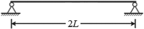
Let us assume that there exists a beam with a length of $2L$, where the cross-sectional area of $A$ is uniform. The dimensionless coordinate $\xi =x/L$ is introduced. The origin of the coordinate is located at the midpoint of the symmetric beam. Then, $-1\le \xi \le 1$. The dimensionless dynamic equation of the beam’s transverse vibration is expressed as follows: (1) $\frac{{\text{d}}^2}{\text{d}{\xi }^2}\left[r\left(\xi \right)\frac{{\text{d}}^{2}W\left(\xi \right)}{\text{d}{\xi }^2}\right]-\lambda \rho \left(\xi \right)W\left(\xi \right)=0.$(1) Here, $r\left(\xi \right)=E\left(\xi \right)J\left(\xi \right)$ is a flexural stiffness function, $\rho \left(\xi \right)$ is a linear density function, $W\left(\xi \right)$ is the displacement mode and $\lambda ={\omega }^2{L}^{4}A$ is the eigenvalue of this problem (Figure 1).

Figure 1. Symmetric simply supported beam about midpoint.

Unlike [13,14], if the coordinate origin is at the midpoint of the beam, the line density $\rho \left(\xi \right)$ and the flexural stiffness $r\left(\xi \right)$ of the symmetric beam are taken as polynomial functions containing an even power, as follows: (2) $\rho \left(\xi \right)=\sum _{i=0}^m{a}_i{\xi }^{2i},r\left(\xi \right)=\sum _{i=0}^n{b}_i{\xi }^{2i},$(2) where m and n are positive integers. The first item on the left side of Equation (1) contains the four order derivative; therefore, $n=m+2$.

The boundary conditions of the simply supported beam can be expressed as follows: (3) $W\left(\pm 1\right)=0,W^{\mathrm{\prime \prime }}\left(\pm 1\right)=0.$(3) The dimensionless coordinates of the nodes for the third-order vibration mode of the symmetric simply supported beam are assumed to be $\pm c\left(0<c<1\right)$, and $W\left(\pm c\right)=0$ exists. Additionally, the dimensionless coordinates of the nodes of the fourth-order vibration mode of the symmetric simply supported beam are assumed to be (a) zero, (b) $\pm d\left(0<d<1\right)$, so that following conditions are satisfied: $W\left(0\right)=0$ and $W\left(\pm d\right)=0$. From the study [15], one concludes that the nodes of the third-order vibration mode and the fourth-order vibration mode of the symmetric simply supported beam alternate with each other; therefore, $0<c<d<1$. The third-order vibration mode satisfying the boundary conditions is expressed by Equation (3) and is denoted by the subscript $\text{T}$. The fourth-order vibration mode is denoted by subscript $\text{F}$. These modes read, respectively, (4) $\left\{\begin{array}{l}{W}_{\text{T}}\left(\xi \right)=B\left({\alpha }_0+{\alpha }_1{\xi }^2+{\alpha }_2{\xi }^4+{\xi }^6\right),\\ W_{\text{F}}\left(\xi \right)=C\xi \left({\beta }_0+{\beta }_1{\xi }^2+{\beta }_2{\xi }^4+{\xi }^6\right).\end{array}\right.$(4) In the above equation, B and C are arbitrary non-zero constants. Additionally, the following relationships hold: (5) $\begin{array}{rl}{\alpha }_0& =\frac{5c^4-9c^2}{5-c^2},{\alpha }_1=\frac{-6c^4+9c^2+9}{5-c^2},{\alpha }_2=\frac{c^4+c^2-14}{5-c^2}.\end{array}$(5) (6) $\begin{array}{rl}{\beta }_0& =\frac{7d^4-11d^2}{7-3d^2},{\beta }_1=\frac{-10d^4+11d^2+11}{7-3d^2},{\beta }_2=\frac{3d^4+3d^2-18}{7-3d^2}.\end{array}$(6) In this paper, we discuss a novel approach toward reconstructing the flexural stiffness $r\left(\xi \right)$ of a symmetric simply supported beam when the line density distribution function $\rho \left(\xi \right)$, displacement mode $W_{\text{T}}\left(\xi \right)$ or $W_{\text{F}}\left(\xi \right)$, and the corresponding natural circle frequency $\omega$ are known, and an approach toward ensuring the positive values of both $\rho \left(\xi \right)$ and $r\left(\xi \right)$.

3. Reconstructing flexural stiffness of symmetric simply supported beam from third-order mode and given linear density functions

3.1. Basic equations

For the first form of Equation (4), the second-order derivative is obtained as follows: (7) $W_{\text{T}}^{\mathrm{\prime \prime }}\left(\xi \right)=B\left(2{\alpha }_1+12{\alpha }_2{\xi }^2+30{\xi }^4\right).$(7) Equations (2) and (7) are substituted into Equation (1) to result in (8) ${\left[\sum _{i=0}^{m+2}{b}_i{\xi }^{2i}\left(2{\alpha }_1+12{\alpha }_2{\xi }^2+30{\xi }^4\right)\right]}^{\mathrm{\prime \prime }}=\lambda \sum _{i=0}^m{a}_i{\xi }^{2i}\left({\alpha }_0+{\alpha }_1{\xi }^2+{\alpha }_2{\xi }^4+{\xi }^6\right).$(8) Equation (8) can be rewritten as follows: (9) $\begin{array}{rl}& 2{\alpha }_1\sum _{i=1}^{m+2}2i\left(2i-1\right)b_i{\xi }^{2i-2}+12{\alpha }_2\sum _{i=0}^{m+2}\left(2i+2\right)\left(2i+1\right)b_i{\xi }^{2i}\\ & +30\sum _{i=0}^{m+2}\left(2i+4\right)\left(2i+3\right)b_i{\xi }^{2i+2}\\ & =\lambda \sum _{i=0}^m{a}_i{\xi }^{2i}\left({\alpha }_0+{\alpha }_1{\xi }^2+{\alpha }_2{\xi }^4+{\xi }^6\right).\end{array}$(9) Equation (9) is valid for an arbitrary $\xi \in \left[-1,1\right]$. By using the coefficient comparison method, we obtain the following equations: (10) $\begin{array}{rl}& 24{\alpha }_2{b}_0+4{\alpha }_1{b}_1=\lambda {\alpha }_0{a}_0,\end{array}$(10) (11) $\begin{array}{rl}& 360b_0+144{\alpha }_2{b}_1+24{\alpha }_1{b}_2=\lambda \left({\alpha }_1{a}_0+{\alpha }_0{a}_1\right),\end{array}$(11) (12) $\begin{array}{rl}& 900b_1+360{\alpha }_2{b}_2+60{\alpha }_1{b}_3=\lambda \left({\alpha }_2{a}_0+{\alpha }_1{a}_1+{\alpha }_0{a}_2\right),\end{array}$(12) (13) $\begin{array}{rl}& \left(2i+2\right)\left(2i+1\right)\left(30b_{i-1}+12{\alpha }_2{b}_i+2{\alpha }_1{b}_{i+1}\right)\\ & =\lambda \left(a_{i-3}+{\alpha }_2{a}_{i-2}+{\alpha }_1{a}_{i-1}+{\alpha }_0{a}_i\right),\left(i=3,4,\dots ,m\right),\end{array}$(13) (14) $\begin{array}{rl}& \left(2m+4\right)\left(2m+3\right)\left(30b_m+12{\alpha }_2{b}_{m+1}+2{\alpha }_1{b}_{m+2}\right)=\lambda \left(a_{m-2}+{\alpha }_2{a}_{m-1}+{\alpha }_1{a}_m\right),\end{array}$(14) (15) $\begin{array}{rl}& \left(2m+6\right)\left(2m+5\right)\left(30b_{m+1}+12{\alpha }_2{b}_{m+2}\right)=\lambda \left(a_{m-1}+{\alpha }_2{a}_m\right),\end{array}$(15) (16) $\begin{array}{rl}& \left(2m+8\right)\left(2m+7\right)30b_{m+2}=\lambda a_m.\end{array}$(16)

Equations (11)–(16) can be expressed as the following matrix equation: (17) $\mathit{D}\mathit{b}=\lambda \mathit{C}\mathit{a}.$(17) In Equation (17), $\mathit{a}=\left(a_0,a_1,a_2,\dots ,a_{m-1},a_m\right)$ is an $m+1$ dimensional column vector, $\mathit{b}=\left(b_0,b_1,b_2,\dots ,b_{m+1},b_{m+2}\right)$ is an $m+3$ dimensional column vector; D is an $m+3$ order square matrix; C is an $m+3$ row and $m+1$ column matrix. $\begin{array}{rl}\mathit{D}& =\left[\begin{array}{ccccc}360& 144{\alpha }_2& 24{\alpha }_1& & \\ & 900& 360{\alpha }_2& 60{\alpha }_1& \\ & & 1680& 672{\alpha }_2& 112{\alpha }_1\\ & & & \ddots & \ddots \\ & & & & 30\left(2m+4\right)\left(2m+3\right)\\ & 0& & & \\ & & & & \end{array}\right.\\ & \left.\begin{array}{cc}& \\ 0& \\ & \\ \ddots & \\ 12\left(2m+4\right)\left(2m+3\right){\alpha }_2& 2\left(2m+4\right)\left(2m+3\right){\alpha }_1\\ 30\left(2m+6\right)\left(2m+5\right)& 12\left(2m+6\right)\left(2m+5\right){\alpha }_2\\ & 30\left(2m+8\right)\left(2m+7\right)\end{array}\right],\\ \mathit{C}& =\left[\begin{array}{cccccc}{\alpha }_1& {\alpha }_0& & & & \\ {\alpha }_2& {\alpha }_1& {\alpha }_0& & 0& \\ 1& {\alpha }_2& {\alpha }_1& {\alpha }_0& & \\ & \ddots & \ddots & \ddots & \ddots & \\ & & 1& {\alpha }_2& {\alpha }_1& {\alpha }_0\\ & & & 1& {\alpha }_2& {\alpha }_1\\ & 0& & & 1& {\alpha }_2\\ & & & & & 1\end{array}\right].\end{array}$

Due to the fact that $\mathit{D}$ is an upper triangular matrix, its inverse ${\mathit{D}}^{-1}$ obviously exists. Thus the following relationship holds: (18) $\mathit{b}=\lambda {\mathit{D}}^{-1}\mathit{C}\mathit{a}\mathbf{.}$(18) In other words, there exists a formal solution to the inverse problem. Note that Equation (10) is a redundant equation and thus can be discarded. Substituting the obtained values of obtaining $b_0$ and $b_1$ into Equation (10), we arrive at $f\left(a_0,a_1,\dots ,a_m;{\alpha }_0,{\alpha }_1,{\alpha }_2\right)=0.$ Since $b_0$ and $b{}_1$ constitute linear functions of $a_0,a_1,\dots ,a_m$, and ${\alpha }_0,{\alpha }_1,{\alpha }_2$ are the functions of the node position dimensionless coordinate $c$, the above equation can be put in the following form: (19) $f_0\left(c\right)a_0+f_1\left(c\right)a_1+\cdots +f_m\left(c\right)a_m=0.$(19) Equation (19) is hereinafter referred as the constraint equation. Only when $a_0,a_1,\dots ,a_m$ satisfy this equation, the formal solution obtained above is the solution of the inverse problem. Below, will be shown that when c is taken from a certain interval, not only does a solution to the inverse problem exist but also the obtained $r\left(\xi \right)$ constitutes a positive function.

3.2. Special cases

As special cases of Equation (17), $m=0,1,2$ are discussed separately in the following sections.

If $m=0$, n turns out to be $n=2$, $\rho \left(\xi \right)=a_0$ and $r\left(\xi \right)=b_0+b_1{\xi }^2+b_2{\xi }^4.$

In this case, Equation (17) becomes $\left[\begin{array}{ccc}360& 144{\alpha }_2& 24{\alpha }_1\\ 0& 900& 360{\alpha }_2\\ 0& 0& 1680\end{array}\right]\cdot \left[\begin{array}{c}{b}_0\\ b_1\\ b_2\end{array}\right]=\lambda a_0\left[\begin{array}{c}{\alpha }_1\\ {\alpha }_2\\ 1\end{array}\right].$ The solution is expressed as follows: $b_2=\frac{\lambda a_0}{1680},b_1=\frac{11\lambda a_0{\alpha }_2}{12,600},b_0=\left(\frac{23{\alpha }_1}{8400}-\frac{11{\alpha }_2^2}{31,500}\right)\lambda a_0.$ The corresponding constraint equation reads $f_0\left(c\right)a_0=0.$ Here, the following relationship holds: (20) $f_0\left(c\right)=\frac{545{\alpha }_1{\alpha }_2-66{\alpha }_2^3-7875{\alpha }_0}{7875}.$(20) One can easily check that function $f_0\left(c\right)$ monotonically increases in the interval of $\left(0,1\right)$ and has only a zero point $c_0$. The numerical solution is obtained as follows: $c_0^2\approx 0.1231\text{or}{c}_0\approx \mathrm{0.3508.}$ If $c=c_0$, we can just let $a_0>0$. The inverse problem then has the following positive solution: $r\left(\xi \right)=\lambda a_0\left(2.7857-2.4804{\xi }^2+0.5952{\xi }^4\right)/1000.$ If $m=1$, the value of n turns out to equal $n=3$; and $\rho \left(\xi \right)=a_0+a_1{\xi }^2$ and $r\left(\xi \right)=b_0+b_1{\xi }^2+b_2{\xi }^4+b_3{\xi }^6.$

In this case, Equation (17) becomes $\left[\begin{array}{cccc}360& 144{\alpha }_2& 24{\alpha }_1& 0\\ 0& 900& 360{\alpha }_2& 60{\alpha }_1\\ 0& 0& 1680& 672{\alpha }_2\\ 0& 0& 0& 2700\end{array}\right]\cdot \left[\begin{array}{c}{b}_0\\ b_1\\ b_2\\ b_3\end{array}\right]=\lambda \left[\begin{array}{cc}{\alpha }_1& {\alpha }_0\\ {\alpha }_2& {\alpha }_1\\ 1& {\alpha }_2\\ 0& 1\end{array}\right]\cdot \left[\begin{array}{c}{a}_0\\ a_1\end{array}\right].$ The solution is expressed as follows: $\begin{array}{rl}{b}_3& =\frac{\lambda a_1}{2700},b_2=\frac{\lambda a_0}{1680}+\frac{169{\alpha }_2\lambda a_1}{378000}{b}_1=\frac{11{\alpha }_2\lambda a_0}{12600}+\left(\frac{11{\alpha }_1}{10125}-\frac{169{\alpha }_2^2}{945000}\right)\lambda a_1,\\ b_0& =\left(\frac{23{\alpha }_1}{8400}-\frac{11{\alpha }_2^2}{31500}\right)\lambda a_0+\left(\frac{{\alpha }_0}{360}-\frac{2633{\alpha }_1{\alpha }_2}{5670000}+\frac{169{\alpha }_2^3}{2362500}\right)\lambda a_1.\end{array}$ The corresponding constraint equation becomes $f_0\left(c\right)a_0+f_1\left(c\right)a_1=0.$ Note that $f_0\left(c\right)$ has been given in Equation (20), while the following relationship holds: (21) $f_1\left(c\right)=\frac{118125{\alpha }_0{\alpha }_2+7700{\alpha }_1^2-21015{\alpha }_1{\alpha }_2^2+3042{\alpha }_2^4}{1771875}.$(21) The variation of the functions $f_0\left(c\right)$ and $f_1\left(c\right)$ with c in the interval of $\left(0,1\right)$ is shown in Figure 2.

Figure 2. Plan of two functions $f_0\left(c\right)$ and $f_1\left(c\right)$.

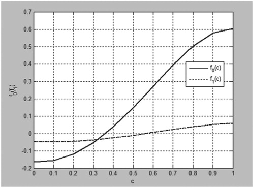
The function $f_1\left(c\right)$ monotonically increases in the interval of $\left(0,1\right)$ and has a unique zero point at $c=c_1$; the numerical solution is given by $c_1^2\approx 0.2898\text{or}{c}_1\approx \mathrm{0.5384.}$ Additionally, the unique solution to the equation $f_0\left(c\right)=f_1\left(c\right)$ in the interval of $\left(0,1\right)$ is given by $c_{01}$ $c_{01}^2\approx 0.0994\text{or}{c}_{01}\approx \mathrm{0.3153.}$ Thus, by using the method proposed in [12], we can draw the following conclusion. If $c_{01}<c<c_1$, $0.3153<c<0.5384,$ and positive solutions exist for the posed inverse problem.

In fact, if $c_{01}<c<c_1$, $a_0>0$ is selected, in the present situation, the following relationship holds: $a_1=-\left[f_0\left(c\right)/f_1\left(c\right)\right]a_0\ge 0.$ Thus we obtain the following relationships: $\rho \left(\xi \right)>0,r\left(\xi \right)=a_0{F}_0\left(\xi ,c\right)+a_1{F}_1\left(\xi ,c\right),$ where $\begin{array}{rl}\frac{F_0\left(\xi ,c\right)}{\lambda }& =\left(\frac{23{\alpha }_1}{8400}-\frac{11{\alpha }_2^2}{31500}\right)+\frac{11{\alpha }_2}{12600}{\xi }^2+\frac{1}{1680}{\xi }^4,\\ \frac{F_1\left(\xi ,c\right)}{\lambda }& =\left(\frac{{\alpha }_0}{360}-\frac{2633{\alpha }_1{\alpha }_2}{5670000}+\frac{169{\alpha }_2^3}{2362500}\right)\\ & +\left(\frac{11{\alpha }_1}{10125}-\frac{169{\alpha }_2^2}{945000}\right){\xi }^2+\frac{169{\alpha }_2}{378000}{\xi }^4+\frac{1}{2700}{\xi }^6.\end{array}$ From Figure 3, one concludes that $F_0\left(\xi ,c\right)$ and $F_1\left(\xi ,c\right)$ are both positive functions in the two-dimensional region $\left(\xi ,c\right)\in \left[0,1\right]\times \left(c_0,c_1\right)$; therefore, $r\left(\xi \right)>0.$

Figure 3. Variation of functions $F_0\left(\xi ,c\right)$ and $F_1\left(\xi ,c\right)$ in two-dimensional region $\left(\xi ,c\right)\in \left[0,1\right]\times \left(c_0,c_1\right)$.

If $c_{01}<c<c_0$ and $a_0>0$ are selected, then the following relationship holds: $a_1=-\left[f_0\left(c\right)/f_1\left(c\right)\right]a_0<0,\text{but}|a_1|<a_0.$ Thus $\rho \left(\xi \right)>0$ also exists. According to Figure 4, it can be verified in a similar manner that the following relationship holds: $r\left(\xi \right)=a_0{F}_0\left(\xi ,c\right)+a_1{F}_1\left(\xi ,c\right)>a_0\left[F_0\left(\xi ,c\right)-F_1\left(\xi ,c\right)\right]>0.$ Generally, as long as $c_{01}<c<c_1$, a positive solution exists for the inverse problem.

Figure 4. Variation of function $F_0\left(\xi ,c\right)-F_1\left(\xi ,c\right)$ in two-dimensional region $\left(\xi ,c\right)\in \left[0,1\right]\times \left(c_0,c_1\right).$

Consider now the case $m=2$. One gets $n=4.$ Moreover, $\rho \left(\xi \right)=a_0+a_1{\xi }^2+a_2{\xi }^4,r\left(\xi \right)=b_0+b_1{\xi }^2+b_2{\xi }^4+b_3{\xi }^6+b_4{\xi }^8.$ In this case, Equation (17) becomes $\left[\begin{array}{ccccc}360& 144{\alpha }_2& 24{\alpha }_1& 0& 0\\ 0& 900& 360{\alpha }_2& 60{\alpha }_1& 0\\ 0& 0& 1680& 672{\alpha }_2& 112{\alpha }_1\\ 0& 0& 0& 2700& 1080{\alpha }_2\\ 0& 0& 0& 0& 3960\end{array}\right]\cdot \left[\begin{array}{c}{b}_0\\ b_1\\ b_2\\ b_3\\ b_4\end{array}\right]=\lambda \left[\begin{array}{ccc}{\alpha }_1& {\alpha }_0& 0\\ {\alpha }_2& {\alpha }_1& {\alpha }_0\\ 1& {\alpha }_2& {\alpha }_1\\ 0& 1& {\alpha }_2\\ 0& 0& 1\end{array}\right]\cdot \left[\begin{array}{c}{a}_0\\ a_1\\ a_2\end{array}\right].$ The solution is obtained as follows: $\begin{array}{rl}{b}_4& =\frac{\lambda a_2}{3960},b_3=\frac{\lambda a_1}{2700}+\frac{2{\alpha }_2\lambda a_2}{7425},b_2=\frac{\lambda a_0}{1680}+\frac{169{\alpha }_2\lambda a_1}{378000}+\left(\frac{481{\alpha }_1}{831600}-\frac{4{\alpha }_2^2}{37125}\right)\lambda a_2,\\ b_1& =\frac{11{\alpha }_2\lambda a_0}{12600}+\left(\frac{11{\alpha }_1}{10125}-\frac{169{\alpha }_2^2}{945000}\right)\lambda a_1+\left(\frac{{\alpha }_0}{900}-\frac{311{\alpha }_1{\alpha }_2}{1247400}+\frac{8{\alpha }_2^3}{185625}\right)\lambda a_2,\\ b_0& =\left(\frac{23{\alpha }_1}{8400}-\frac{11{\alpha }_2^2}{31500}\right)\lambda a_0+\left(\frac{{\alpha }_0}{360}-\frac{2633{\alpha }_1{\alpha }_2}{5670000}+\frac{169{\alpha }_2^3}{2362500}\right)\lambda a_1\\ & +\left(-\frac{{\alpha }_0{\alpha }_2}{2250}-\frac{481{\alpha }_1^2}{12474000}+\frac{1667{\alpha }_1{\alpha }_2^2}{15592500}+\frac{16{\alpha }_2^4}{928125}\right)\lambda a_2.\end{array}$

Thus the following relationship holds: $r\left(\xi \right)=a_0{F}_0\left(\xi ,c\right)+a_1{F}_1\left(\xi ,c\right)+a_2{F}_2\left(\xi ,c\right).$ Here, $F_0\left(\xi ,c\right)$ and $F_1\left(\xi ,c\right)$ have been given above, and the following relationship holds (Figure 5): $\begin{array}{rl}\frac{F_2\left(\xi ,c\right)}{\lambda }& =\left(-\frac{{\alpha }_0{\alpha }_2}{2250}-\frac{481{\alpha }_1^2}{12474000}+\frac{1667{\alpha }_1{\alpha }_2^2}{15592500}-\frac{16{\alpha }_2^4}{928125}\right)\\ & +\left(\frac{{\alpha }_0}{900}-\frac{311{\alpha }_1{\alpha }_2}{1247400}+\frac{8{\alpha }_2^3}{185625}\right){\xi }^2\\ & +\left(\frac{481{\alpha }_1}{831600}-\frac{4{\alpha }_2^2}{37125}\right){\xi }^4+\frac{2{\alpha }_2}{7425}{\xi }^6+\frac{1}{3960}{\xi }^8.\end{array}$ The corresponding constraint equation is expressed as follows: $f_0\left(c\right)a_0+f_1\left(c\right)a_1+f_2\left(c\right)a_2=0.$ Here, $f_0\left(c\right)$ and $f_1\left(c\right)$ have been given in Equations (20) and (21), respectively, and the following relationship holds: (22) $f_2\left(c\right)=\frac{86625{\alpha }_0{\alpha }_1-207900{\alpha }_0{\alpha }_2^2-37475{\alpha }_1^2{\alpha }_2+53370{\alpha }_1{\alpha }_2^3-8064{\alpha }_2^5}{19490625}.$(22) Function $f_2\left(c\right)$ has a unique zero point $c_2$ in the interval of $\left(0,1\right)$, and the numerical solution can be obtained as follows: $c_2^2\approx 0.4043or{c}_2\approx \mathrm{0.6359.}$ According to the discussion presented in Section 2.2.2, if $c_1\le c<c_2$, $a_0>0$ and $a_1>0$ are selected, then, $a_2=-{\left[f_0\left(c\right)a_0+f_1\left(c\right)a_1\right]/f}_2\left(c\right)>0.$ If $c_{01}<c<c_1$, $a_0>0$ is selected, $a_2$ is selected as a positive number that is smaller than $a_0$, and we select $a_1=-\left[f_0\left(c\right)a_0+f_2\left(c\right)a_2\right]/f_1\left(c\right)=a_{10}+a_{12}.$ Then, if $c_0\le c<c_1$, $a_1>0$. Additionally, if $c_{01}<c<c_0$, $|a_{10}|<a_0$. Thus, a detailed conclusion can be drawn, according to which, if $c_{01}<c<c_2$, then, $0.3153<c<0.6359$, approximately. Therefore, positive solutions exist for the inverse problems.

The above discussion can be extended to the situation of $m\ge 3$. Generally, the node is taken at $c=1/3.$ Moreover, we can expect that special circumstances apply for $m=0,$ and positive solutions exist for the inverse problems. An example is presented below.

Figure 5. Variation of function $F_2\left(\xi ,c\right)$ in a two-dimensional region $\left(\xi ,c\right)\in \left[0,1\right]\times \left(c_{01},c_2\right).$

Example 1. If coefficients $a_i$ are known and $\rho \left(\xi \right)$ is given, one needs to calculate $b_i$. This process allows one to obtain $r\left(\xi \right)$. If, for example, $c=1/3$ is selected, then ${\alpha }_0=-19/99,{\alpha }_1=67/33,$ ${\alpha }_2=-281/99.$ If in Equations (11)–(16), $m=4$ is selected, one obtains $\lambda =990.$ Thus we can obtain the following relationship: $\left[\begin{array}{c}{b}_0\\ b_1\\ b_2\\ b_3\\ b_4\\ b_5\\ b_6\end{array}\right]=\left[\begin{array}{ccccc}2.7183& 0.5021& 0.2265& 0.1193& 0.0695\\ -2.4532& 0.7573& 0.2356& 0.1197& 0.0695\\ 0.5893& -1.2563& 0.3032& 0.1231& 0.0697\\ 0& 0.3667& -0.7569& 0.1480& 0.0711\\ 0& 0& 0.2500& -0.5037& 0.0819\\ 0& 0& 0& 0.1813& -0.3585\\ 0& 0& 0& 0& 0.1375\end{array}\right]\cdot \left[\begin{array}{c}{a}_0\\ a_1\\ a_2\\ a_3\\ a_4\end{array}\right].$ The corresponding constraint equation is expressed as follows: $1494.588a_0+2777.2932a_1+1338.0936a_2+708.3204a_3+412.83a_4=0.$ It can be seen that just by taking $a_0$ as a positive number, $a_2$, $a_3$ and $a_4$ are positive numbers and relatively smaller than $a_0$. Now, if we select $a_1$ as follows: $a_1=-\frac{1494.588a_0+1338.0936a_2+708.3204a_3+412.83a_4}{2777.2932},$ then $\begin{array}{rl}\rho \left(\xi \right)& =a_0\left(1-\frac{1494.588}{2777.2932}{\xi }^2\right)+a_2{\xi }^2\left({\xi }^2-\frac{1338.0936}{2777.2932}\right)\\ & +a_3{\xi }^2\left({\xi }^4-\frac{708.3204}{2777.2932}\right)+a_4{\xi }^2\left({\xi }^6-\frac{412.83}{2777.2932}\right)\end{array}$ constitutes a positive function. Additionally, under the selection method of $a_i(i=0,1,2,3,4),$ although $a_1$ is negative, it still satisfies the inequality $|a_1|<a_0$; therefore, the following function is also positive: $r\left(\xi \right)=a_0{F}_0\left(\xi ,1/3\right)+a_1{F}_1\left(\xi ,1/3\right)+a_2{F}_2\left(\xi ,1/3\right)+a_3{F}_3\left(\xi ,1/3\right)+a_4{F}_4\left(\xi ,1/3\right).$ In above equation, $F_i\left(\xi ,1/3\right)\left(i=0,1,2,3,4\right)$ is the particular solution to column i of the coefficient matrix in the above solution. Thus it is easy to verify the positive values of these special solutions and the $F_0\left(\xi ,1/3\right)-F_1\left(\xi ,1/3\right)$ function.

3.3. Well-posedness of the solution

The solution is well-posed because it exists, is unique, and stable. The existence of the solution is discussed in Section 2.1. It is straightforward to see from Section 2.1 that the solution of the inverse problem is unique as long as the selected node location c is located within the interval satisfying the constraint Equation (19). In the following paragraph, the stability of the solution will be mainly illuminated.

In fact, the solution of the above inverse problem depends on three types of known quantities: the given mass distribution function $\rho \left(\xi \right)$, the given mode of vibration $W_{\text{T}}\left(\xi \right)$ and the corresponding eigenvalue $\lambda$. Equation (18) shows that the coefficient vector $\mathit{b}$ of the solution is obviously linearly dependent on the eigenvector $\lambda$ and the coefficient vector $\mathit{a}$ of the mass distribution function. Therefore, when these two types of quantities change slightly, the corresponding solution $r\left(\xi \right)$ will only change slightly, i.e. the solution is stable to the changes of these two types of quantities. Moreover, we investigated the expressions of the $W_{\text{T}}\left(\xi \right)$ mode and found that their coefficients are only related to the dimensionless coordinate c of the node location. From Equation (5), because $0<c<1$, the coefficients ${\alpha }_0,{\alpha }_1,{\alpha }_2$ of $W_{\text{T}}\left(\xi \right)$ are all continuously differentiable functions of c. In the expression of matrices $\mathit{C}$ and $\mathit{D}$ in the solution expressed by Equation (18), it can be seen that the matrix elements are also continuously differentiable functions of c. Moreover, it can be seen that $\mathit{D}$ is an upper triangular matrix, and that the principal diagonal elements are independent constant coefficients of $c$. Hence, the elements of ${\mathit{D}}^{-1}$ are also continuously differentiable functions of c. Therefore, as a composite function of c, the coefficient vector $\mathit{b}$ of the solution must be a continuously differentiable function of c, and the special case presented in Section 2.2 also verifies this conclusion. Therefore, the solution $r\left(\xi \right)$ is stable to the change of the node position c.

In conclusion, the solution of the inverse problem obtained in this section is well-posed.

4. Reconstructing flexural stiffness of symmetric simply supported beam from fourth-order mode and given linear density functions

4.1. Basic equations

For the second form of Equation (4), the two order derivative can be obtained as follows: (23) $W_F^{\mathrm{\prime \prime }}\left(\xi \right)=C\left(6d_1\xi +20d_2{\xi }^3+42{\xi }^5\right).$(23) Equations (2) and (23) are substituted into Equation (1) as follows: (24) ${\left[\sum _{i=0}^{m+2}{b}_i{\xi }^{2i}\left(6{\beta }_1\xi +20{\beta }_2{\xi }^3+42{\xi }^5\right)\right]}^{\mathrm{\prime \prime }}=\lambda \sum _{i=0}^m{a}_i{\xi }^{2i}\left({\beta }_0\xi +{\beta }_1{\xi }^3+{\beta }_2{\xi }^5+{\xi }^7\right).$(24) Equation (24) can be rewritten as follows: (25) $\begin{array}{rl}& 6{\beta }_1\sum _{i=1}^{m+2}\left(2i+1\right)2i{b}_i{\xi }^{2i-1}+20{\beta }_2\sum _{i=0}^{m+2}\left(2i+3\right)\left(2i+2\right)b_i{\xi }^{2i+1}\\ & +42\sum _{i=0}^{m+2}\left(2i+5\right)\left(2i+4\right)b_i{\xi }^{2i+3}\\ & =\lambda \sum _{i=0}^m{a}_i{\xi }^{2i}\left({\beta }_0\xi +{\beta }_1{\xi }^3+{\beta }_2{\xi }^5+{\xi }^7\right).\end{array}$(25) Equation (25) is established for an arbitrary $\xi \in \left[-1,1\right]$. By using the comparison coefficient method, we can obtain the following relationships: (26) $\begin{array}{rl}& 120{\beta }_2{b}_0+36{\beta }_1{b}_1=\lambda {\beta }_0{a}_0,\end{array}$(26) (27) $\begin{array}{rl}& 840b_0+400{\beta }_2{b}_1+120{\beta }_1{b}_2=\lambda \left({\beta }_1{a}_0+{\beta }_0{a}_1\right),\end{array}$(27) (28) $\begin{array}{rl}& 1764b_1+840{\beta }_2{b}_2+252{\beta }_1{b}_3=\lambda \left({\beta }_2{a}_0+{\beta }_1{a}_1+{\beta }_0{a}_2\right),\end{array}$(28) (29) $\begin{array}{rl}& \left(2i+3\right)\left(2i+2\right)\left(42b_{i-1}+20{\beta }_2{b}_i+6{\beta }_1{b}_{i+1}\right)\\ & =\lambda \left(a_{i-3}+{\beta }_2{a}_{i-2}+{\beta }_1{a}_{i-1}+{\beta }_0{a}_i\right),\left(i=3,4,\dots ,m\right),\end{array}$(29) (30) $\begin{array}{rl}& \left(2m+5\right)\left(2m+4\right)\left(42b_m+20{\beta }_2{b}_{m+1}+6{\beta }_1{b}_{m+2}\right)=\lambda \left(a_{m-2}+{\beta }_2{a}_{m-1}+{\beta }_1{a}_m\right),\end{array}$(30) (31) $\begin{array}{rl}& \left(2m+7\right)\left(2m+6\right)\left(42b_{m+1}+20{\beta }_2{b}_{m+2}\right)=\lambda \left(a_{m-1}+{\beta }_2{a}_m\right),\end{array}$(31) (32) $\begin{array}{rl}& \left(2m+9\right)\left(2m+8\right)42b_{m+2}=\lambda a_m.\end{array}$(32)

Equations (27)–(32) can be written as a matrix equation, as follows: (33) $\mathit{F}\mathit{b}=\lambda \mathit{E}\mathit{a}.$(33) In Equation (33), $\mathit{a}$ and $\mathit{b}$ are column vectors that are still defined in the previous section; F is an $m+3$ order square matrix; E is an $m+3$ row and $m+1$ column matrix. $\begin{array}{rl}\mathit{F}& =\left[\begin{array}{cccc}840& 400{\beta }_2& 120{\beta }_1& \\ & 1764& 840{\beta }_2& 252{\beta }_1\\ & & 3024& 1440{\beta }_2\\ & & \ddots & \ddots \\ & & & 42\left(2m+5\right)\left(2m+4\right)\\ & 0& & \\ & & & \end{array}\right.\\ & \left.\begin{array}{cc}& \\ & 0\\ 432{\beta }_1& \\ \ddots & \\ 20\left(2m+5\right)\left(2m+4\right){\beta }_2& 6\left(2m+5\right)\left(2m+4\right){\beta }_1\\ 42\left(2m+7\right)\left(2m+6\right)& 20\left(2m+7\right)\left(2m+6\right){\beta }_2\\ & 42\left(2m+9\right)\left(2m+8\right)\end{array}\right],\\ E& =\left[\begin{array}{cccccc}{\beta }_1& {\beta }_0& & & & \\ {\beta }_2& {\beta }_1& {\beta }_0& & 0& \\ 1& {\beta }_2& {\beta }_1& {\beta }_0& & \\ & \ddots & \ddots & \ddots & \ddots & \\ & & 1& {\beta }_2& {\beta }_1& {\beta }_0\\ & & & 1& {\beta }_2& {\beta }_1\\ & 0& & & 1& {\beta }_2\\ & & & & & 1\end{array}\right].\end{array}$

In the same way as in the previous section, matrix $\mathit{F}$ has an inverse matrix $\mathit{Y}$. Then, Equation (33) can be rewritten as follows: (34) $\mathit{b}=\lambda \mathit{Y}\mathit{E}\mathit{a}.$(34) In other words, formal solutions to an inverse problem exist. Additionally, in the same way as in the previous section, Equation (26) is a redundant equation and is called the constraint equation corresponding to the fourth-order modes. This equation can eventually be written as follows: (35) $g_0\left(c\right)a_0+g_1\left(c\right)a_1+\cdots +g_m\left(c\right)a_m=0.$(35) Only when $a_0,a_1,\dots ,a_m$ satisfy the above equation, the obtained formal solution is actually the solution of the inverse problem.

4.2. Special case

The establishment of Equation (33) requires $m\ge 3$; $m=0,1,2$ is discussed separately in the following sections.

If $m=0$, n turns to equal $n=2$; $\rho \left(\xi \right)=a_0$ and $r\left(\xi \right)=b_0+b_1{\xi }^2+b_2{\xi }^4.$ $[\left(b_0+b_1{\xi }^2+b_2{\xi }^4\right)\cdot \left(6{\beta }_1\xi +20{\beta }_2{\xi }^3+42{\xi }^5\right){]}^{\mathrm{\prime \prime }}=\lambda a_0\left({\beta }_0\xi +{\beta }_1{\xi }^3+{\beta }_2{\xi }^5+{\xi }^7\right).$ By the comparison coefficient method, the following relationship is obtained: $\left[\begin{array}{ccc}840& 400{\beta }_2& 120{\beta }_1\\ 0& 1764& 840{\beta }_2\\ 0& 0& 3024\end{array}\right]\cdot \left[\begin{array}{c}{b}_0\\ b_1\\ b_2\end{array}\right]=\lambda a_0\left[\begin{array}{c}{\beta }_1\\ {\beta }_2\\ 1\end{array}\right].$ The solution reads $b_2=\frac{\lambda a_0}{3024},b_1=\frac{13\lambda {\beta }_2{a}_0}{31752},b_0=\frac{121\lambda {\beta }_1{a}_0}{105840}-\frac{65\lambda {\beta }_2^2{a}_0}{333396}.$ The corresponding constraint equation is expressed as follows: (36) $g_0\left(d\right)a_0=0,$(36) where $g_0\left(d\right)=\frac{67{\beta }_1{\beta }_2}{441}-\frac{650{\beta }_2^3}{27783}-{\beta }_0.$ Equation (36) has a unique zero point $d_0$ in the interval of $(0,1)$. The numerical solution is obtained as follows: $d_0^2\approx 0.2873\text{or}{d}_0\approx \mathrm{0.5360.}$ We take this value as a node; accordingly, the following functions both take positive values: $\rho \left(\xi \right)=a_0,r\left(\xi \right)=\lambda a_0\left(1.0074-1.1266{\xi }^2+0.3307{\xi }^4\right)/1000.$ For $m=1,$ $n=3$; $\rho \left(\xi \right)=a_0+a_1{\xi }^2,r\left(\xi \right)=b_0+b_1{\xi }^2+b_2{\xi }^4+b_3{\xi }^6$ and $\begin{array}{rl}& [\left(b_0+b_1{\xi }^2+b_2{\xi }^4+b_3{\xi }^6\right)\cdot \left(6{\beta }_1\xi +20{\beta }_2{\xi }^3+42{\xi }^5\right){]}^{\mathrm{\prime \prime }}\\ & =\lambda \left(a_0+a_1{\xi }^2\right)\cdot \left({\beta }_0\xi +{\beta }_1{\xi }^3+{\beta }_2{\xi }^5+{\xi }^7\right).\end{array}$ By the comparison coefficient method, the following relationship is derived: $\left[\begin{array}{cccc}840& 400{\beta }_2& 120{\beta }_1& 0\\ 0& 1764& 840{\beta }_2& 252{\beta }_1\\ 0& 0& 3024& 1440{\beta }_2\\ 0& 0& 0& 4620\end{array}\right]\cdot \left[\begin{array}{c}{b}_0\\ b_1\\ b_2\\ b_3\end{array}\right]=\lambda \left[\begin{array}{cc}{\beta }_1& {\beta }_0\\ {\beta }_2& {\beta }_1\\ 1& {\beta }_2\\ 0& 1\end{array}\right]\cdot \left[\begin{array}{c}{a}_0\\ a_1\end{array}\right].$ The solution is expressed as follows: $\begin{array}{rl}{b}_3& =\frac{\lambda a_1}{4620},b_2=\frac{\lambda a_0}{3024}+\frac{53\lambda {\beta }_2{a}_1}{232848},b_1=\frac{13{\beta }_2}{31752}\lambda a_0+\left(\frac{13{\beta }_1}{24255}-\frac{265{\beta }_2^2}{2444904}\right)\lambda a_1,\\ b_0& =\left(\frac{121{\beta }_1}{105840}-\frac{65{\beta }_2^2}{333396}\right)\lambda a_0+\left(\frac{{\beta }_0}{840}+\frac{1325{\beta }_2^3}{25671492}-\frac{67{\beta }_1{\beta }_2}{232848}\right)\lambda a_1.\end{array}$ Thus the solution of corresponding inverse problem is $r\left(\xi \right)=a_0{G}_0\left(\xi ,d\right)+a_1{G}_1\left(\xi ,d\right),$ where $\begin{array}{rl}\frac{G_0\left(\xi ,d\right)}{\lambda }& =\left(\frac{121{\beta }_1}{105840}-\frac{65{\beta }_2^2}{333396}\right)+\frac{13{\beta }_2}{31752}{\xi }^2+\frac{1}{3024}{\xi }^4,\\ \frac{G_1\left(\xi ,d\right)}{\lambda }& =\left(\frac{{\beta }_0}{840}-\frac{67{\beta }_1{\beta }_2}{232848}+\frac{1325{\beta }_2^3}{25671492}\right)\\ & +\left(\frac{13{\beta }_1}{24255}-\frac{265{\beta }_2^2}{2444904}\right){\xi }^2+\frac{53{\beta }_2}{232848}{\xi }^4+\frac{1}{4620}{\xi }^6.\end{array}$ By substituting these relationships into the constraint equation (26), the following relationship is arrived at (37) $g_0\left(d\right)a_0+g_1\left(d\right)a_1=0,$(37) where $g_0\left(d\right)$ has been given in Equation (36). Moreover, $g_1\left(d\right)=\frac{{\beta }_0{\beta }_2}{7}+\frac{52{\beta }_1^2}{2695}-\frac{145{\beta }_1{\beta }_2^2}{3773}+\frac{13250{\beta }_2^4}{2139291}.$ Equation (37) has a unique root $d_1$ in the interval of $\left(0,1\right)$, its numerical value being: $d_1^2\approx 0.3810d_1\approx \mathrm{0.6173.}$ Additionally, the unique solution to equation $g_0\left(d\right)=g_1\left(d\right)$ in the interval of $(0,1)$ is $d_{01}$: $d_{01}^2\approx 0.2436\text{or}{d}_{01}\approx \mathrm{0.4936.}$ Thus we can draw the following conclusion: if $d_{01}<d<d_1$, then 0.4936 < d < 0.6173. Moreover, positive solutions exist for the inverse problem at hand.

For $m=2,n=4;$ $\rho \left(\xi \right)=a_0+a_1{\xi }^2+a_2{\xi }^4$ and $r\left(\xi \right)=b_0+b_1{\xi }^2+b_2{\xi }^4+b_3{\xi }^6+b_4{\xi }^8.$ Substitution into governing differential equation yields $\begin{array}{rl}& [\left(b_0+b_1{\xi }^2+b_2{\xi }^4+b_3{\xi }^6+b_4{\xi }^8\right)\cdot \left(6{\beta }_1\xi +20{\beta }_2{\xi }^3+42{\xi }^5\right){]}^{\mathrm{\prime \prime }}\\ & =\lambda \left(a_0+a_1{\xi }^2+a_2{\xi }^4\right)\cdot \left({\beta }_0\xi +{\beta }_1{\xi }^3+{\beta }_2{\xi }^5+{\xi }^7\right).\end{array}$

By the comparison coefficient method, the following relationship is obtained as $\left[\begin{array}{ccccc}840& 400{\beta }_2& 120{\beta }_1& 0& 0\\ 0& 1764& 840{\beta }_2& 252{\beta }_1& 0\\ 0& 0& 3024& 1440{\beta }_2& 432{\beta }_1\\ 0& 0& 0& 4620& 2200{\beta }_2\\ 0& 0& 0& 0& 6552\end{array}\right]\cdot \left[\begin{array}{c}{b}_0\\ b_1\\ b_2\\ b_3\\ b_4\end{array}\right]=\lambda \left[\begin{array}{ccc}{\beta }_1& {\beta }_0& 0\\ {\beta }_2& {\beta }_1& {\beta }_0\\ 1& {\beta }_2& {\beta }_1\\ 0& 1& {\beta }_2\\ 0& 0& 1\end{array}\right]\cdot \left[\begin{array}{c}{a}_0\\ a_1\\ a_2\end{array}\right].$ The solution reads $\begin{array}{rl}{b}_4& =\frac{\lambda a_2}{6552},b_3=\frac{\lambda a_1}{4620}+\frac{136\lambda {\beta }_2{a}_2}{945945},\\ b_2& =\frac{\lambda a_0}{3024}+\frac{53{\beta }_2\lambda a_1}{232848}+\left(\frac{85{\beta }_1}{275184}-\frac{272{\beta }_2^2}{3972969}\right)\lambda a_2,\\ b_1& =\frac{13{\beta }_2}{1764}\lambda a_0+\left(\frac{52{\beta }_1}{24255}-\frac{265{\beta }_2^2}{2444904}\right)\lambda a_1+\left(\frac{{\beta }_0}{1764}+\frac{2720{\beta }_2^3}{83432349}-\frac{26639{\beta }_1{\beta }_2}{158918760}\right)\lambda a_2,\\ b_0& =\left(\frac{121{\beta }_1}{105840}-\frac{65{\beta }_2^2}{18522}\right)\lambda a_0+\left(\frac{{\beta }_0}{840}-\frac{1717{\beta }_1{\beta }_2}{1629936}+\frac{1325{\beta }_2^3}{25671492}\right)\lambda a_1\\ & +\left(-\frac{5{\beta }_0{\beta }_2}{18522}-\frac{85{\beta }_1^2}{1926288}+\frac{29903{\beta }_1{\beta }_2^2}{333729396}-\frac{27200{\beta }_2^4}{1752079329}\right)\lambda a_2.\end{array}$

Thus the following relationship holds: $r\left(\xi \right)=a_0{G}_0\left(\xi ,d\right)+a_1{G}_1\left(\xi ,d\right)+a_2{G}_2\left(\xi ,d\right).$ Here, $G_0\left(\xi ,d\right)$ and $G_1\left(\xi ,d\right)$ have been given above, and the following relationship holds: $\begin{array}{rl}\frac{G_2\left(\xi ,d\right)}{\lambda }& =\left(-\frac{5{\beta }_0{\beta }_2}{18522}-\frac{85{\beta }_1^2}{1926288}+\frac{29903{\beta }_1{\beta }_2^2}{333729396}-\frac{27200{\beta }_2^4}{1752079329}\right)\\ & +\left(\frac{{\beta }_0}{1764}-\frac{26639{\beta }_1{\beta }_2}{158918760}+\frac{2720{\beta }_2^3}{83432349}\right){\xi }^2\\ & +\left(\frac{85{\beta }_1}{275184}-\frac{272{\beta }_2^2}{3972969}\right){\xi }^4+\frac{136{\beta }_2}{945945}{\xi }^6+\frac{1}{6552}{\xi }^8.\end{array}$ By substituting $b_1$ and $b_0$ into the constraint equation (26), the following relationship exists: $g_0\left(d\right)a_0+g_1\left(d\right)a_1+g_2\left(d\right)a_2=0.$ In the above equation, $g_0\left(d\right)$ and $g_1\left(d\right)$ have been given in Equations (36) and (37), respectively, and the following relationship holds: (38) $g_2\left(d\right)=\frac{{\beta }_0{\beta }_1}{49}-\frac{100{\beta }_0{\beta }_2^2}{3087}-\frac{25007{\beta }_1^2{\beta }_2}{2207205}+\frac{331670{\beta }_1{\beta }_2^3}{27810783}-\frac{1088000{\beta }_2^5}{584026443}.$(38) Function $g_2\left(d\right)$ has a unique zero point $d_2$ in the interval of $\left(0,1\right)$, and a numerical solution can be obtained as follows: $d_2^2\approx 0.4747\text{or}{d}_2\approx \mathrm{0.6890.}$ According to the discussion presented in the previous section, we can conclude that, if $d_{01}<d<d_2,$ $0.4936<d<0.6890,$ approximately, and positive solutions exist for the inverse problems.

The discussion above can be extended to the case of $m\ge 3$. Generally, the same can be observed in the node taken at $d=1/2;$ we expect the special circumstances of $m=0,$ and positive solutions exist for the inverse problems. Another example is given as follows.

Example 2. Similar to Example 1, if $a_i$ is known and $\rho \left(\xi \right)$ is given, we want to calculate $b_i$, and then $r\left(\xi \right)$ is also obtained. If $d=1/2$ is selected, then ${\beta }_0=-0.37,{\beta }_1=2.1,{\beta }_2=-\mathrm{2.73.}$ Additionally, if $m=4$ and $\lambda =3000$ are selected, from Equation (34), the following relationship exists: $\left[\begin{array}{c}{b}_0\\ b_1\\ b_2\\ b_3\\ b_4\\ b_5\\ b_6\end{array}\right]=\left[\begin{array}{ccccc}2.8433& 0.4770& 0.2184& 0.1262& 0.0793\\ -3.3532& 0.9532& 0.2638& 0.1317& 0.0801\\ 0.9921& -1.8642& 0.4152& 0.1501& 0.0827\\ 0& 0.6494& -1.1775& 0.2114& 0.0911\\ 0& 0& 0.4579& -0.8078& 0.1194\\ 0& 0& 0& 0.3401& -0.5872\\ 0& 0& 0& 0& 0.2626\end{array}\right]\cdot \left[\begin{array}{c}{a}_0\\ a_1\\ a_2\\ a_3\\ a_4\end{array}\right].$ The corresponding constraint equation is expressed as follows: $74.967a_0+84.2032a_1+51.60456a_2+31.3866a_3+19.92312a_4=0.$ It can be seen that by just taking $a_0$ as a positive number, then $a_2$, $a_3$ and $a_4$ are positive numbers relatively smaller than $a_0$, and $a_1$ is selected as follows: $a_1=-\frac{74.967a_0+51.60456a_2+31.3866a_3+19.92312a_4}{84.20328}.$ Then, in the same way as in Example 1 given in the previous section, $\begin{array}{rl}\rho \left(\xi \right)& =a_0\left(1-\frac{74.967}{84.20328}{\xi }^2\right)+a_2{\xi }^2\left({\xi }^2-\frac{51.60456}{84.20328}\right)\\ & +a_3{\xi }^2\left({\xi }^4-\frac{31.3866}{84.20328}\right)+a_4{\xi }^2\left({\xi }^6-\frac{19.92312}{84.20328}\right)\end{array}$ and $r\left(\xi \right)=a_0{G}_0\left(\xi ,1/2\right)+a_1{G}_1\left(\xi ,1/2\right)+a_2{G}_2\left(\xi ,1/2\right)+a_3{G}_3\left(\xi ,1/2\right)+a_4{G}_4\left(\xi ,1/2\right)$ will both be positive functions. In the above equation, $G_i\left(\xi ,1/2\right)\left(i=0,1,2,3,4\right)$ is the particular solution to column i of the coefficient matrix in the above solution.

4.3. Well-posedness of solution

Similar to the discussion presented in Section 2.3, the existence and uniqueness of the solution of the inverse problem is straightforward. With regard to stability, as can be seen in Equation (6), because $0<d<1$ exists, the coefficients ${\beta }_0,{\beta }_1,{\beta }_2$ of $W_{\text{F}}\left(\xi \right)$ are all continuously differentiable functions of d. Because the inference process discussed in Section 3.1 is completely similar to that discussed in Section 2.1, the coefficient vector $\mathit{b}$ of the solution in Equation (34) is also linearly dependent on the eigenvalues $\lambda$ and coefficient vector $\mathit{a}$ of the mass distribution function $\rho \left(\xi \right)$. Additionally, this is a continuously differentiable function of d, and the special case presented in Section 3.2 also verifies this fact. Therefore, the solution $r\left(\xi \right)$ is stable for three types of known quantities.

5. Discussion

Owing to the symmetric structure, beam possesses only two displacement modes: the symmetric mode and the anti-symmetric mode, which are equivalent to two associated half-length structures [15]. The half-length structure corresponding to the symmetrical mode is a single-span beam with a sliding end on the left, and a pinned end on the right. Additionally, the half-length structure corresponding to the anti-symmetric mode is a single-span beam with two pinned ends. Therefore, the higher order modes mentioned in this paper are actually the second-order modes of two different half-length structures. Thus the discussion presented in this paper can also be extended to a beam with a sliding-pinned end and a beam with two pinned ends.

6. Conclusion

In this paper, we discuss the conditions required for constructing the flexural stiffness of a symmetric simply supported beam using the symmetric mode or anti-symmetric mode. Similarly, we also consider higher order modes, such as the fifth-order mode, sixth-order mode and symmetric polynomial type flexural stiffness to construct the linear density function of symmetric simply supported beams. It is shown that the calculation process becomes more complicated as the mode-order increases.

Acknowledgements

This study was supported by the Anhui Provincial Natural Science Foundation under Grant Nos. 1808085MA05, 1808085MA20 and 1708085MA10. We thank Liwen Bianji, Edanz Editing China (www.liwenbianji.cn/ac), for editing the English text of a draft of this manuscript.

Disclosure statement

No potential conflict of interest was reported by the authors.

References

- Loy CT, Lam KY, Reddy JN. Vibration of functionally graded cylindrical shells. Int J Mech Sci. 1999;41(3):309–324. doi: 10.1016/S0020-7403(98)00054-X
- Yang J, Shen MS. Free vibration and parametric resonance of shear deformable functionally graded cylindrical panels. J Sound Vib. 2003;261(5):871–893. doi: 10.1016/S0022-460X(02)01015-5
- Yang J, Shen MS. Dynamic response of initially stressed functionally graded rectangular thin plates. Compos Struct. 2001;54(4):497–508. doi: 10.1016/S0263-8223(01)00122-2
- Chen WQ, Ding HJ. On free vibration of a functionally graded piezoelectric rectangular plate. Acta Mech. 2002;153(3):207–216. doi: 10.1007/BF01177452
- Kim KS, Noda N. Green's function approach to unsteady thermal stresses in an infinite hollow cylinder of functionally graded material. Acta Mech. 2002;156(3):145–161. doi: 10.1007/BF01176753
- Akgöz B, Civalek Ö. Buckling analysis of functionally graded microbeams based on the strain gradient theory. Acta Mech. 2013;224(9):2185–2201. doi: 10.1007/s00707-013-0883-5
- Elishakoff I, Candan S. Apparently first closed-form solution for vibrating: inhomogeneous beams. Int J Solids Struct. 2001;38:3411–3441. doi: 10.1016/S0020-7683(00)00266-3
- Elishakoff I, Candan S. Apparently first closed-form solution for frequencies of deterministically and /or stochastically inhomogeneous simply supported beams. J Appl Mech. 2001;68(3):176–185.
- Elishakoff I. Eigenvalues of inhomogeneous structures: unusual closed-form solutions. Boca Raton: CRC Press; 2004.
- Wu L, Wang Q, Elishakoff I. Semi-inverse method for axially functionally graded beams with an anti-symmetric vibration mode. J Sound Vib. 2005;284(3):1190–1202. doi: 10.1016/j.jsv.2004.08.038
- Wu L, Zhang L, Wang Q, et al. Reconstructing cantilever beams via vibration mode with a given node location. Acta Mech. 2011;217(1):135–148.
- He M, Zhang L, Wang Q. Reconstructing cross-sectional physical parameters for two-span beams with overhang using fundamental mode. Acta Mech. 2014;225(2):349–359. doi: 10.1007/s00707-013-0963-6
- Wang Q, Liu M, Zhang L, et al. Reconstruction flexural stiffness of symmetric simply supported beams with single mode. J Comput Phys. 2014;31(2):216–222.
- He M, Zhang L, Huang Z, et al. Reconstructing the axial stiffness of a symmetric rod with two elastic supports using single mode. Acta Mech. 2017;228(4):1511–1524. doi: 10.1007/s00707-016-1783-2
- Wang D, Wang Q, He B. Qualitative theory in structural mechanics. Beijing: Peking University Press; 2014, pp. 235–237.