A general spatial multi-loop linkage optimization model for motion generation with static loading

ABSTRACT

A general spatial multi-loop linkage optimization model for the inverse problem of defect-free motion generation is formulated and demonstrated in this work. The particular linkage of focus is the Revolute-Spherical-Spherical-Revolute-Spherical-Spherical joint (or RSSR-SS) linkage: one of the most basic spatial multi-loop linkages in terms of construction and kinematics. With this optimization model, the RSSR-SS linkage dimensions required to approximate precision positions are calculated along with the driving link torque required to achieve static equilibrium for precision position forces. The optimization model also includes constraints to eliminate order, branch and circuit defects-defects that are common in classical dyad-based dimensional synthesis. Therefore, the novelty of this work is the development of a general optimization model for RSSR-SS motion generation with static loading that simultaneously considers order, branch and circuit defect elimination. This work conveys both the benefits and drawbacks realized when implementing the RSSR-SS optimization model on a personal computer using the commercial mathematical analysis software package Matlab.

KEYWORDS:

• RSSR-SS linkage
• motion generation
• static loading
• constrained nonlinear optimization
• Matlab

1. Introduction

1.1. The RSSR-SS linkage

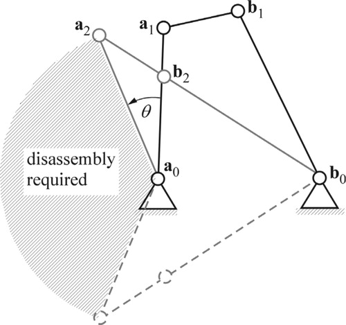
The Revolute-Spherical-Spherical-Revolute-Spherical-Spherical joint or RSSR-SS linkage (Figure 1) is a particular type of spatial multi-loop linkage. As illustrated in Figure 1, the coupler link of this linkage is supported by three links (2 R-S links and 1 S-S link). In comparison, the coupler link of four-bar linkages is supported by only two links. The additional coupler link support in the RSSR-SS linkage makes it more capable of supporting loads in comparison to single-loop four-bar spatial linkages and as a result, more structurally sound.

Figure 1. RSSR-SS linkage (left) with joint descriptions and (right) with displacement variables.

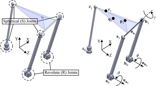
The RSSR-SS linkage is one of the most basic spatial multi-loop linkages in terms of construction and kinematics. Regarding basic construction, the RSSR-SS linkage is comprised of only 5 links interconnected by 2 revolute joints and 4 spherical joints. In addition, this linkage requires no specific construction scheme for assembly (in comparison to the four-bar spherical linkage with requires that all joint axes have a common intersection point). Regarding basic kinematics, fully-controlled coupler link motion of the RSSR-SS linkage is achieved by controlling the rotation of a single revolute joint. As illustrated in Figure 1, the coupler link includes ${\mathbf{p}}_1$, ${\mathbf{q}}_1$ and ${\mathbf{r}}_1$. The RSSR-SS linkage is a simpler, lower-cost alternative to the six degree of freedom robotic Stewart platform manipulator [1].

1.2. Developments in RSSR-SS linkage design and analysis

Contributions in the areas of RSSR-SS linkage design and analysis include a computer-aided method to synthesize order and branch defect-free RSSR-SS linkages to achieve four partially exact and partially approximate coupler positions [2]. A method was presented for the synthesis of adjustable RSSR-SS linkages to approximate both prescribed coupler positions and prescribed coupler velocities and accelerations [3]. A combined analytical-numerical model was developed for the kinematic displacement analysis of RSSR-SS linkages [4]. Also, a fully analytical model was developed for the kinematic displacement and velocity analysis of RSSR-SS linkages [5].

So RSSR-SS design methods such as defect-free motion generation, motion generation with prescribed coupler velocities and kinematic motion analysis have all been addressed in published works. The RSSR-SS method being addressed in this work however is defect-free RSSR-SS motion generation with static structural loading.

1.3. Spatial motion generation with static structural loading

The objective in motion generation is to calculate the linkage dimensions required to approximate user-prescribed link positions (called precision positions). Motion generation has traditionally been exclusively kinematic in focus-considering motion without respect to forces.

While a kinematic analysis is among the most fundamental analyses to consider in mechanical design, there is an order of progression among analyses in mechanical design. Beyond a kinematic analysis is the static structural analysis-the most fundamental analysis to consider in mechanical design where structural loading is included.

By including static loading constraints in a motion generation optimization model, one can not only calculate the linkage dimensions required to approximate precision positions, but also calculate the driving link torque required to achieve static equilibrium at the precision positions given loads at these positions.

Optimization models for defect-free motion generation with static structural loading have already been presented for spatial single-loop linkages such as the Spherical four-bar linkage, the RRSS linkage and the RRSC linkage [6–9]. However, because the RSSR-SS linkage (being a multi-loop spatial linkage) is more structurally sound than any single-loop spatial linkage, it would make a more suitable linkage of focus for defect-free spatial motion generation with static structural loading. In this work, a general optimization model is developed and demonstrated for defect-free RSSR-SS motion generation with static structural loading the first time.

1.4. Motivation and scope of work

The motivation for this work includes the dearth of design tools available for optimal RSSR-SS motion generation. Also motivating this work is the need to simultaneously consider defect elimination within motion generation to ensure that RSSR-SS designs are calculated that are free of order, branch and circuit defects. Lastly, the relevance of static structural analysis in the design of mechanical systems also motivates this work.

The novelty of this work is the first-time development of a general optimization model for RSSR-SS motion generation with static loading that simultaneously considers order, branch and circuit defect elimination. This work also conveys both the benefits and the drawbacks associated with the general RSSR-SS optimization model and its implementation in the commercial mathematical analysis software package Matlab on a personal computer.

2. Kinematic displacement and velocity models for the RSSR-SS linkage

2.1. RSSR-SS displacement model

A fully-analytical kinematic displacement model was presented for the RSSR-SS linkage [5]. The displacements of moving pivots ${\mathbf{a}}_1$ and ${\mathbf{b}}_1$ result from the rotation of links ${\mathbf{a}}_0-{\mathbf{a}}_1$ and ${\mathbf{b}}_0-{\mathbf{b}}_1$ about their fixed-pivot joint axes by displacement angles $\theta$ and $\phi$ (Figure 1). The displacements of ${\mathbf{a}}_1$ and ${\mathbf{b}}_1$ are given by (1) $\mathbf{a}=\left[R_{\theta ,{\mathbf{u}}_{{\mathbf{a}}_0}}\right]\left({\mathbf{a}}_1-{\mathbf{a}}_0\right)+{\mathbf{a}}_0$(1) (2) $\mathbf{b}=\left[R_{\mathrm{\varnothing },{\mathbf{u}}_{{\mathbf{b}}_0}}\right]\left({\mathbf{b}}_1-{\mathbf{b}}_0\right)+{\mathbf{b}}_0$(2)

In these equations, $\left[R_{\theta ,{\mathbf{u}}_{{\mathbf{a}}_0}}\right]$ and $\left[R_{\phi ,{\mathbf{u}}_{{\mathbf{b}}_0}}\right]$ are 3 × 3 spatial rotation matrices about the fixed pivot axis vectors ${\mathbf{u}}_{{\mathbf{a}}_0}$ and ${\mathbf{u}}_{{\mathbf{b}}_0}$ respectively (Figure 1). The general form of the spatial rotation matrix (considering a rotation axis vector $\mathbf{u}$ and a displacement angle $\delta$) is (3) $\left[R_{\delta ,\mathbf{u}}\right]=\left[\begin{array}{ccc}{u}_x^{2}v\left(\delta \right)+\cos \left(\delta \right)& u_x^{}{u}_y^{}v\left(\delta \right)-u_z^{}\sin \left(\delta \right)& u_x^{}{u}_z^{}v\left(\delta \right)+u_y^{}\sin \left(\delta \right)\\ u_x^{}{u}_y^{}v\left(\delta \right)+u_z^{}\sin \left(\delta \right)& u_y^{2}v\left(\delta \right)+\cos \left(\delta \right)& u_y^{}{u}_z^{}v\left(\delta \right)-u_x^{}\sin \left(\delta \right)\\ u_x^{}{u}_z^{}v\left(\delta \right)-u_y^{}\sin \left(\delta \right)& u_y^{}{u}_z^{}v\left(\delta \right)-u_x^{}\sin \left(\delta \right)& u_z^{2}v\left(\delta \right)+\cos \left(\delta \right)\end{array}\right]$(3) where $v\left(\delta \right)=1-\cos \left(\delta \right)$.

The RSSR-SS kinematic displacement model is completed by including equations for the displacements of RSSR-SS moving pivot ${\mathbf{c}}_1$ and coupler point ${\mathbf{p}}_1$ (Figure 1) [5]. These equations are (4) $\begin{array}{rl}\mathbf{c}& =\left[R_{\gamma ,{\mathbf{u}}_{\mathbf{a}}}\right]\left[R_{\omega ,\mathbf{w}}\right]\left(\left[R_{\theta ,{\mathbf{u}}_{{\mathbf{a}}_0}}\right]\left({\mathbf{c}}_1-{\mathbf{a}}_0\right)+{\mathbf{a}}_0-\mathbf{a}\right)+\mathbf{a}\end{array}$(4) (5) $\begin{array}{rl}\mathbf{p}& =\left[R_{\gamma ,{\mathbf{u}}_{\mathbf{a}}}\right]\left[R_{\omega ,\mathbf{w}}\right]\left(\left[R_{\theta ,{\mathbf{u}}_{{\mathbf{a}}_0}}\right]\left({\mathbf{p}}_1-{\mathbf{a}}_0\right)+{\mathbf{a}}_0-\mathbf{a}\right)+\mathbf{a}\end{array}$(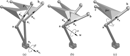5) It can be observed from the given spatial rotation matrices $\left[R_{\theta ,{\mathbf{u}}_{{\mathbf{a}}_0}}\right]$, $\left[R_{\omega ,\mathbf{w}}\right]$ and $\left[R_{\gamma ,{\mathbf{u}}_{\mathbf{a}}}\right]$ that three distinct and simultaneous rotations comprise a coupler link displacement in the RSSR-SS linkage [5]. These rotations and their corresponding rotation axis vectors are illustrated in Figure 2. The coupler link rotates about the driving link fixed pivot axis vector ${\mathbf{u}}_{{\mathbf{a}}_0}$ by the driving link displacement angle $\theta$. This rotation displaces the moving pivot ${\mathbf{a}}_1$ and the axis ${\mathbf{u}}_{{\mathbf{a}}_1}$ to $\mathbf{a}$ and ${{\mathbf{u}}^{\mathrm{\prime }}}_{{\mathbf{a}}_1}$ respectively (Figure 2a). The coupler link also rotates about a vector $\mathbf{w}$ by a displacement angle $\omega$. Vector $\mathbf{w}$ is a unit vector orthogonal to the plane including vectors ${\mathbf{u}}_{{\mathbf{a}}_{\text{1}}}$ and ${{\mathbf{u}}^{\mathrm{\prime }}}_{{\mathbf{a}}_1}$. This rotation achieves the final moving pivot location $\mathbf{b}$ and displaces the axis ${{\mathbf{u}}^{\mathrm{\prime }}}_{{\mathbf{a}}_1}$ to ${\mathbf{u}}_{\mathbf{a}}$ (Figure 2b). Lastly, the coupler rotates about a vector ${\mathbf{u}}_{\mathbf{a}}$ by a displacement angle $\gamma$. This rotation achieves the final moving pivot location $\mathbf{c}$ and coupler point location $\mathbf{p}$ (Figure 2c).

Figure 2. RSSR-SS (a) $\theta -{\mathbf{u}}_{{\mathbf{a}}_0}$, (b) $\omega -\mathbf{w}$ and (c) $\gamma -{\mathbf{u}}_{\mathbf{a}}$ coupler rotations.

Vector ${\mathbf{u}}_{\mathbf{a}}$ is produced by the displaced moving pivots $\mathbf{a}$ and $\mathbf{b}$(therefore ${\mathbf{u}}_{\mathbf{a}}=\left(\mathbf{b}-\mathbf{a}\right)/||\mathbf{b}-\mathbf{a}||$). Additionally, vector $\mathbf{w}$ (a coupler rotation axis vector formed by the cross product ${{\mathbf{u}}^{\mathrm{\prime }}}_{{\mathbf{a}}_1}\times {\mathbf{u}}_{\mathbf{a}}$) is defined as (6) $\mathbf{w}=\frac{{{\mathbf{u}}^{\mathrm{\prime }}}_{{\mathbf{a}}_1}\times {\mathbf{u}}_{\mathbf{a}}}{|{{\mathbf{u}}^{\mathrm{\prime }}}_{{\mathbf{a}}_1}\times {\mathbf{u}}_{\mathbf{a}}|}$(6) where (7) ${{\mathbf{u}}^{\mathrm{\prime }}}_{{\mathbf{a}}_1}=\left[R_{\theta ,{\mathbf{u}}_{{\mathbf{a}}_0}}\right]{\mathbf{u}}_{{\mathbf{a}}_1}$(7)

Vector ${\mathbf{u}}_{{\mathbf{a}}_1}$ is produced by the initial moving pivots ${\mathbf{a}}_1$ and ${\mathbf{b}}_1$ (therefore ${\mathbf{u}}_{{\mathbf{a}}_{\text{1}}}=\left({\mathbf{b}}_{\text{1}}-{\mathbf{a}}_1\right)/||{\mathbf{b}}_{\text{1}}-{\mathbf{a}}_1||$). Being spatial rotation matrices, both $\left[R_{\omega ,\mathbf{w}}\right]$ and $\left[R_{\gamma ,{\mathbf{u}}_{\mathbf{a}}}\right]$ are identical in form to Equation (3).

The RSSR-SS variables ${\mathbf{a}}_0$, ${\mathbf{a}}_1$, ${\mathbf{u}}_{{\mathbf{a}}_0}$, ${\mathbf{b}}_0$, ${\mathbf{b}}_1$, ${\mathbf{u}}_{{\mathbf{b}}_0}$, ${\mathbf{c}}_0$, ${\mathbf{c}}_1$ and ${\mathbf{p}}_1$ are all 3 × 1 vectors containing natural coordinates-spatial Cartesian x, y and z-components. Coupler point ${\mathbf{p}}_1$ as well as coupler points ${\mathbf{q}}_1$ and ${\mathbf{r}}_1$ (which are introduced in Section 5) are three arbitrarily-chosen nonlinear points used to describe the spatial position of the rigid-body affixed to the coupler in the initial mechanism position. As the linkage is driven, these points are displaced along with the rigid-body.

In practice, coupler points ${\mathbf{p}}_1$, ${\mathbf{q}}_1$ and ${\mathbf{r}}_1$ are selected from the geometry of the coupler link. The Cartesian coordinates of these points could be easily measured, for example, from the coupler link geometry when modeled using computer-aided design software. Because there are no restrictions on where the three points could be measured on the coupler link as long as they form a plane (three coincident or linear points don’t achieve this), these points are selected according to the user’s own preferences.

2.2. RSSR-SS velocity model

A fully-analytical kinematic velocity model was also presented for the RSSR-SS linkage [5]. This section does not include the entire velocity model, rather just the velocity equations that are needed to formulate the forthcoming static loading constraint in the RSSR-SS optimization model. The reader is encouraged to refer to the Shen et. al. reference for the complete RSSR-SS velocity model [5].

To formulate the forthcoming static loading constraint in the RSSR-SS optimization model, an equation for the velocity of the displaced coupler point ${\mathbf{p}}_1$ (which will be named $\dot{\mathbf{p}}$) is needed. In the RSSR-SS velocity model, the equation formulated for $\dot{\mathbf{p}}$ is (8) $\dot{\mathbf{p}}=\dot{\gamma }\left[P_{{\mathbf{u}}_{\mathbf{a}}}\right]\left(\mathbf{p}-\mathbf{a}\right)+\dot{\omega }\left[P_{\text{w}}\right]\left(\mathbf{p}-\mathbf{a}\right)+\dot{\theta }\left[P_{{\mathbf{u}}_{{\mathbf{a}}_0}}\right]\left(\mathbf{p}-{\mathbf{a}}_{\mathbf{0}}\right)$(8) where (9) $\dot{\gamma }=\frac{-\dot{\omega }{\left(\mathbf{c}-{\mathbf{c}}_0\right)}^T\left[P_{\text{w}}\right]\left(\mathbf{c}-\mathbf{a}\right)-\dot{\theta }{\left(\mathbf{c}-{\mathbf{c}}_0\right)}^T\left[P_{{\mathbf{u}}_{{\mathbf{a}}_0}}\right]\left(\mathbf{c}-{\mathbf{a}}_0\right)}{{\left(\mathbf{c}-{\mathbf{c}}_0\right)}^T\left[P_{{\mathbf{u}}_{\mathbf{a}}}\right]\left(\mathbf{c}-\mathbf{a}\right)}$(9) (10) $\dot{\omega }=\dot{\theta }\frac{{\left(\mathbf{b}-{\mathbf{b}}_0\right)}^T\left\{\frac{{\left(\mathbf{a}\mathbf{-}{\mathbf{a}}_{\mathbf{0}}\right)}^T\left[P_{{\mathbf{u}}_{{\mathbf{a}}_0}}\right]\left(\mathbf{a}-\mathbf{b}\right)}{{\left(\mathbf{a}-\mathbf{b}\right)}^T\left[P_{{\mathbf{u}}_{{\mathbf{b}}_0}}\right]\left(\mathbf{b}-{\mathbf{b}}_0\right)}\left[P_{{\mathbf{u}}_{{\mathbf{b}}_0}}\right]\left(\mathbf{b}-{\mathbf{b}}_0\right)-\left[P_{{\mathbf{u}}_{{\mathbf{a}}_0}}\right]\left(\mathbf{b}-{\mathbf{a}}_0\right)\right\}}{{\left(\mathbf{b}-{\mathbf{b}}_0\right)}^T\left[P_{\text{w}}\right]\left(\mathbf{b}-\mathbf{a}\right)}$(10) and the matrix $\left[P_{\mathbf{u}}\right]$ has the form (11) $\left[P_{\mathbf{u}}\right]=\left[\begin{array}{ccc}0& -u_z& u_y\\ u_z& 0& -u_x\\ -u_y& u_x& 0\end{array}\right]$(11)

Matrix $\left[P_{\mathbf{u}}\right]$ is produced from the derivative of $\left[R_{\delta ,\mathbf{u}}\right]$ in Equation (3): $\frac{\text{d}\left[R_{\delta ,\mathbf{u}}\right]}{dt}=\dot{\delta }\left[P_{\mathbf{u}}\right]$.

3. Branch, order and circuit defects

Although many motion generation approaches ensure that synthesized linkages will achieve or approximate precision positions, they do not guarantee:

1. the synthesized linkage will achieve the precision positions without a change in its original assembly configuration (thus requiring linkage disassembly).

2. the synthesized linkage will achieve the precision positions in the intended order.

3. the synthesized linkage will achieve the precision positions without breaking the linkage closed loop (also requiring linkage disassembly).

These three uncertainties are often fatal defects (in terms of linkage performance) and are inherent in motion generation.

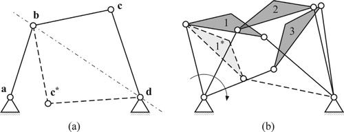
The first noted defect is commonly called the branch defect [10,11]. Figure 3a illustrates the two assembly configurations of a planar four-bar linkage: configurations a-b-c-d and a-b-c-d. In kinematic synthesis, a branch represents the precision positions that are achieved by a single linkage assembly configuration. When both assembly configurations are required to achieve all of the precision positions, this can introduce a potential design problem because the linkage would require disassembly and reassembly from one assembly configuration to the other during operation to achieve all of the precision positions. Figure 3b illustrates a planar four-bar branch defect. In this figure, precision positions 1-2-3 are achieved by planar four-bar configuration a-b-c-d while precision position 1 is achieved by configuration a-b-c-d. So if the design application requires that this linkage achieves the precision positions in the order 1-1-2-3 continuously, this would not be possible with a single mechanism assembly configuration due to the given branch defect.

Figure 3. (a) Four-bar linkage assembly configurations and (b) branch defect.

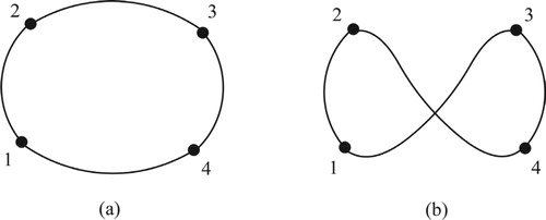
The second noted defect is commonly called the order defect [10,11]. When precision positions or precision points are defined, it is typically desired that the synthesized linkage achieves them in the given order in which they were prescribed. If, for example, the precision points are defined in the order 1-2-3-4-1 (Figure 4a) but the synthesized linkage achieves the points in the order 1-2-4-3-1 (Figure 4b) this can present a potential problem-especially if the prescribed point order is required to trace a particular coupler curve. As shown in Figure 4, the order in which precision positions or precision points are achieved determines the particular coupler path profile or coupler motion sequence achieved.

Figure 4. Order difference with four precision points (orders (a) 1-2-3-4 and (b) 1-2-4-3).

The third noted defect is commonly called the circuit defect [10,11]. While both branch and circuit defects require linkage disassembly to rectify, the reasons for linkage disassembly are distinct. With the branch defect, linkage disassembly is required to go from one linkage assembly configuration to another. With the circuit defect however, linkage disassembly is required to allow linkage motion beyond its limit position for the same assembly configuration. Using the planar four-bar linkage in Figure 5 as an example, when the driving link (link ${\mathbf{a}}_0-{\mathbf{a}}_1$) is rotated by angle $\theta$, it can travel no farther in the counter-clockwise direction unless the linkage is disassembled. Any non-Grashof linkage (a four-bar linkage where the driving link cannot achieve a 360° rotation) will have limit positions. If the driving link of a synthesized linkage must travel beyond its limit positions to achieve its precision positions, linkage disassembly is required.

Figure 5. Four-bar linkage with circuit defect.

4. Formulation of an RSSR-SS linkage static coupler force with driver static torque constraint

If an arbitrary force $\mathbf{F}$ is applied at the displaced coupler point $\mathbf{p}$ of the RSSR-SS linkage, one can conclude from the principal of virtual work that (12) $\mathbf{F}\cdot \dot{\mathbf{p}}=T\dot{\theta }$(12) where $T$ is the torque applied to the driving link (link ${\mathbf{a}}_0-{\mathbf{a}}_1$ in Figure 1). Substituting Equations (9) and (10) into Equation (8), and substituting the resulting equation into Equation (12) produces (13) $T=\mathbf{F}\cdot \left\{\left(-\frac{k_3{k}_5}{k_4{k}_7}-\frac{k{}_6}{k_7}\right)\left[P_{{\mathbf{u}}_{\mathbf{a}}}\right]\left(\mathbf{p}-\mathbf{a}\right)+\frac{k_3}{k_4}\left[P_{\mathbf{w}}\right]\left(\mathbf{p}-\mathbf{a}\right)+\left[P_{{\mathbf{u}}_{{\mathbf{a}}_0}}\right]\left(\mathbf{p}-{\mathbf{a}}_0\right)\right\}$(13) where (14) $\left\{\begin{array}{l}{k}_1={\left(\mathbf{a}-{\mathbf{a}}_0\right)}^T\left[P_{{\mathbf{u}}_{{\mathbf{a}}_0}}\right]\left(\mathbf{a}-\mathbf{b}\right)\\ k_2={\left(\mathbf{a}-\mathbf{b}\right)}^T\left[P_{{\mathbf{u}}_{{\mathbf{b}}_0}}\right]\left(\mathbf{b}-{\mathbf{b}}_0\right)\\ k_3={\left(\mathbf{b}-{\mathbf{b}}_0\right)}^T\left\{\frac{k_1}{k_2}\left[P_{\mathbf{u}{\mathbf{b}}_0}\right]\left(\mathbf{b}-{\mathbf{b}}_0\right)-\left[P_{{\mathbf{u}}_{{\mathbf{a}}_0}}\right]\left(\mathbf{b}-{\mathbf{a}}_0\right)\right\}\\ k_4={\left(\mathbf{b}-{\mathbf{b}}_0\right)}^T\left[P_{\mathbf{w}}\right]\left(\mathbf{b}-\mathbf{a}\right)\\ k_5={\left(\mathbf{c}-{\mathbf{c}}_0\right)}^T\left[P_{\mathbf{w}}\right]\left(\mathbf{c}-\mathbf{a}\right)\\ k_6={\left(\mathbf{c}-{\mathbf{c}}_0\right)}^T\left[P_{{\mathbf{u}}_{{\mathbf{a}}_0}}\right]\left(\mathbf{c}-{\mathbf{a}}_0\right)\\ k_7={\left(\mathbf{c}-{\mathbf{c}}_0\right)}^T\left[P_{{\mathbf{u}}_{\mathbf{a}}}\right]\left(\mathbf{c}-{\mathbf{a}}_0\right)\end{array}\right.$(14) Using Equation (13), the driver torque of the RSSR-SS linkage (required to achieve static equilibrium) is calculated for a coupler force $\mathbf{F}$ applied at the displaced coupler point $\mathbf{p}$.

5. Constrained optimization model for RSSR-SS motion generation with static structural loading

What makes the optimization model here a general model is that the entire general displacement model presented in Section 2.1 is incorporated into it. This optimization model includes the objective function (15) $f\left(\mathbf{X}\right)=\sum _{j=2}^N\left\{{||{\mathbf{p}}_j^{\ast }-{\mathbf{p}}_j^{}||}^2+{||{\mathbf{q}}_j^{\ast }-{\mathbf{q}}_j^{}||}^2+{||{\mathbf{r}}_j^{\ast }-{\mathbf{r}}_j^{}||}^2\right\}$(15) In Equation (15), $\mathbf{X}=({\mathbf{a}}_0,{\mathbf{a}}_1,{\mathbf{u}}_{{\mathbf{a}}_0},{\mathbf{b}}_0,{\mathbf{b}}_1,{\mathbf{u}}_{{\mathbf{b}}_0},{\mathbf{c}}_0,{\mathbf{c}}_1,{\theta }_{1-2}\dots {\theta }_{1-N},{\mathrm{\varnothing }}_{1-2}\dots {\mathrm{\varnothing }}_{1-N},{\gamma }_{1-2}\dots {\gamma }_{1-N})$ which are all of the design variables for the RSSR-SS linkage (Figure 1). Displacement angle variables $\phi$ and $\gamma$ are both dependent on angle $\theta$ since the RSSR-SS linkage has a single degree of freedom. This can be observed in the equations for $\phi$ and $\gamma$ (not included in this work) in the RSSR-SS displacement model that is included in the RSSR-SS optimization model [5]. Variables ${\mathbf{p}}_j^{\ast }$, ${\mathbf{q}}_j^{\ast }$ and ${\mathbf{r}}_j^{\ast }$ in Equation (15) represent the precision position coordinates and variables ${\mathbf{p}}_j^{}$, ${\mathbf{q}}_j^{}$ and ${\mathbf{r}}_j^{}$ include the coupler position coordinates achieved by the synthesized RSSR-SS motion generator. The equations for the displaced coupler points $\mathbf{q}$ and $\mathbf{r}$ are identical in form to Equation (5) where $\mathbf{p}$ and ${\mathbf{p}}_1$ are replaced with $\mathbf{q}$ and ${\mathbf{q}}_1$ respectively (or $\mathbf{r}$ and ${\mathbf{r}}_1$).

Equation (15) allows for the direct minimization of the structural error between the precision positions and the coupler positions achieved by the synthesized RSSR-SS motion generator. An objective function having this capability is ideal for motion generation since, by definition, the objective in motion generation is to replicate precision positions as closely as possible.

Along with the objective function, the optimization model includes three kinds of equality constraints. Equations (16) and (17) are unit vector constraints for joint axis vectors ${\mathbf{u}}_{{\mathbf{a}}_0}$ and ${\mathbf{u}}_{{\mathbf{b}}_0}$ (Figure 1). (16) $\begin{array}{rl}& ({\mathbf{u}}_{{\mathbf{a}}_0}{)}^T\left({\mathbf{u}}_{{\mathbf{a}}_0}\right)-1=0\end{array}$(16) (17) $\begin{array}{rl}& ({\mathbf{u}}_{{\mathbf{b}}_0}{)}^T\left({\mathbf{u}}_{{\mathbf{b}}_0}\right)-1=0\end{array}$(17)

Equations (18) and (19) are orthogonality constraints to ensure that links ${\mathbf{a}}_1-{\mathbf{a}}_0$ and ${\mathbf{b}}_1-{\mathbf{b}}_0$ are orthogonal to joint axis vectors ${\mathbf{u}}_{{\mathbf{a}}_0}$ and ${\mathbf{u}}_{{\mathbf{b}}_0}$ respectively (Figure 1). (18) $\begin{array}{rl}& ({\mathbf{u}}_{{\mathbf{a}}_0}{)}^T\left({\mathbf{a}}_{\text{j}}-{\mathbf{a}}_0\right)=0,j=2\dots N\end{array}$(18) (19) $\begin{array}{rl}& ({\mathbf{u}}_{{\mathbf{b}}_0}{)}^T\left({\mathbf{b}}_{\text{j}}-{\mathbf{b}}_0\right)=0,j=2\dots N\end{array}$(19)

Equations (20) through (25) are constant length constraints for links ${\mathbf{a}}_1-{\mathbf{a}}_0$, ${\mathbf{b}}_1-{\mathbf{b}}_0$, ${\mathbf{c}}_1-{\mathbf{c}}_0$ and coupler link distances ${\mathbf{a}}_1-{\mathbf{b}}_1$, ${\mathbf{a}}_1-{\mathbf{c}}_1$ and ${\mathbf{b}}_1-{\mathbf{c}}_1$ respectively (Figure 1). The displaced moving pivots $\mathbf{a}$, $\mathbf{b}$ and $\mathbf{c}$ are calculated using Equations (1), (2) and (4) from the RSSR-SS kinematic displacement model. (20) $\begin{array}{rl}& ({\mathbf{a}}_{\text{j}}-{\mathbf{a}}_0{)}^T\left({\mathbf{a}}_{\text{j}}-{\mathbf{a}}_0\right)-({\mathbf{a}}_1-{\mathbf{a}}_0{)}^T\left({\mathbf{a}}_1-{\mathbf{a}}_0\right)=0,j=2\dots N\end{array}$(20) (21) $\begin{array}{rl}& ({\mathbf{b}}_{\text{j}}-{\mathbf{b}}_0{)}^T\left({\mathbf{b}}_{\text{j}}-{\mathbf{b}}_0\right)-({\mathbf{b}}_1-{\mathbf{b}}_0{)}^T\left({\mathbf{b}}_1-{\mathbf{b}}_0\right)=0,j=2\dots N\end{array}$(21) (22) $\begin{array}{rl}& ({\mathbf{a}}_{\text{j}}-{\mathbf{b}}_{\text{j}}{)}^T\left({\mathbf{a}}_{\text{j}}-{\mathbf{b}}_{\text{j}}\right)-({\mathbf{a}}_1-{\mathbf{b}}_1{)}^T\left({\mathbf{a}}_1-{\mathbf{b}}_1\right)=0,j=2\dots N\end{array}$(22) (23) $\begin{array}{rl}& ({\mathbf{c}}_{\text{j}}-{\mathbf{c}}_0{)}^T\left({\mathbf{c}}_{\text{j}}-{\mathbf{c}}_0\right)-({\mathbf{c}}_1-{\mathbf{c}}_0{)}^T\left({\mathbf{c}}_1-{\mathbf{c}}_0\right)=0,j=2\dots N\end{array}$(23) (24) $\begin{array}{rl}& ({\mathbf{a}}_{\text{j}}-{\mathbf{c}}_{\text{j}}{)}^T\left({\mathbf{a}}_{\text{j}}-{\mathbf{c}}_{\text{j}}\right)-({\mathbf{a}}_1-{\mathbf{c}}_1{)}^T\left({\mathbf{a}}_1-{\mathbf{c}}_1\right)=0,j=2\dots N\end{array}$(24) (25) $\begin{array}{rl}& ({\mathbf{b}}_{\text{j}}-{\mathbf{c}}_{\text{j}}{)}^T\left({\mathbf{b}}_{\text{j}}-{\mathbf{c}}_{\text{j}}\right)-({\mathbf{b}}_1-{\mathbf{c}}_1{)}^T\left({\mathbf{b}}_1-{\mathbf{c}}_1\right)=0,j=2\dots N\end{array}$(25)

The RSSR-SS optimization model also includes three kinds of inequality constraints. Inequality (26) eliminates branch defects in the RSSR-SS linkage loop ${\mathbf{a}}_0-{\mathbf{a}}_1-{\mathbf{b}}_1-{\mathbf{b}}_0$ because it ensures a constant cross product of link ${\mathbf{b}}_0\mathbf{-}\mathbf{b}$ and distance ${\mathbf{b}}_0\mathbf{-}\mathbf{a}$ [10,11]. A change in branch would result in a change in sign of the cross-products. Likewise, Inequality (27) eliminates branch defects in the RSSR-SS linkage loop ${\mathbf{c}}_0-{\mathbf{c}}_1-0\text{.5}\left({\mathbf{a}}_{\text{1}}\mathbf{+}{\mathbf{b}}_1\right)-0\text{.5}\left({\mathbf{a}}_{\text{0}}\mathbf{+}{\mathbf{b}}_0\right)$. Inequality (28) ensures that the driver torque required for static equilibrium (calculated from Equation (13)) is less than a prescribed maximum driver torque ${\tau }_{max}$. Inequality (29) eliminates order defects [10,11] because it ensures constant counter-clockwise crank rotation (or clockwise rotation if ${\theta }_j<{\theta }_{j-1}$ is used). (26) $\left[\left({\mathbf{b}}_{\text{j}}-{\mathbf{b}}_0\right)\times \left({\mathbf{a}}_{\text{j}}-{\mathbf{b}}_0\right)\right]\cdot \left[\left({\mathbf{b}}_1-{\mathbf{b}}_0\right)\times \left({\mathbf{a}}_1-{\mathbf{b}}_0\right)\right]>0,j=2\dots N$(26) (27) $\left[\left({\mathbf{c}}_{\text{j}}-{\mathbf{c}}_0\right)\times \left(\frac{{\mathbf{a}}_{\text{j}}+{\mathbf{b}}_{\text{j}}}{2}-{\mathbf{c}}_0\right)\right]\cdot \left[\left({\mathbf{c}}_1-{\mathbf{c}}_0\right)\times \left(\frac{{\mathbf{a}}_1+{\mathbf{b}}_1}{2}-{\mathbf{c}}_0\right)\right]>0,j=2\dots N$(27) (28) $|T_j|<{\tau }_{max},j=2,3,\dots ,N$(28) (29) $\left\{\begin{array}{l}{\theta }_j>{\theta }_{j-1}\\ {\theta }_N<2\pi \end{array}\right.,j=2,3,\dots ,N$(29)

This combination of objective function and inequality constraints allows for the direct minimization of precision position error while simultaneously mitigating order and branch defects. The driver torque constraint ensures that static equilibrium will be achieved for selected coupler positions within a maximum driver torque limit. And by including the entire closed-loop displacement model in the optimization model, circuit defects are also mitigated [10,11]. In comparison, defect elimination cannot be ensured in RSSR-SS design methods where individual dyads are calculated and then assembled to produce the RSSR-SS linkage [2,3]. For this work, this general RSSR-SS motion generation model with static loading was implemented in the commercial mathematical analysis software Matlab. This optimization model utilizes natural coordinates-coordinates based on line or quadratic equations (rather than chiefly trigonometric expressions) [12].

6. Optimization model file size comparison in Matlab

The RSSR-SS motion optimization model presented in Section 5 was codified in the commercial mathematical analysis software package Matlab and solved using the interior-point algorithm for constrained nonlinear optimization problems [13]. While the RSSR-SS kinematic models and the RSSR-SS optimization model are given in matrix form in Sections 2 through 4, the full algebraic expansion of these models are required prior to solution calculation in Matlab.

The interior-point algorithm requires both the gradient and the Hessian of a constrained optimization model’s objective function and nonlinear constraints [13]. If the gradients and Hessians are not explicitly provided by the user, they will be estimated in Matlab. But as with any estimation, there is a possibility that it will poorly reflect reality. This possibility becomes more probable as the scale of the optimization model grows. Therefore, the best optimization model gradient and Hessian formulations would be algebraic formulations provided by the user [13]. However, it is when algebraic gradients and Hessians are included in the RSSR-SS optimization model that implementation challenges become evident.

Table 1 includes the files sizes in Matlab of the fully-expanded RSSR-SS optimization model, its gradients and its Hessians formulated for 2 precision positions. The total file size of the fully-expanded optimization model (the $f\left(\mathbf{X}\right)$ column in Table 1) is 43.318 megabytes. An optimization model of this size is very manageable in Matlab on a 64-bit personal computer in terms of the memory required for solution calculation. The total size of the fully-expanded optimization model and gradients (the $\mathrm{\nabla }f$ column in Table 1) is 14.4 gigabytes. An optimization model of this size poses a significant challenge in Matlab on a 64-bit personal computer. However, the total size of the fully-expanded optimization model and gradients and Hessians (the $\mathbf{H}\left(f\right)$ column in Table 1) is 265 gigabytes-a size that makes the complete optimization impractical for use in Matlab on even high-end personal computers.

Table 1. Equation, Gradient and Hessian File Sizes (in MB for $N=2$ coupler positions) in Matlab.

Eq. No.	$f\left(\mathbf{X}\right)$	$\mathrm{\nabla }f$	$\mathbf{H}\left(f\right)$
15 (for 2 pos.)	2.564	847.304	*18954
16	0.001	0.001	0.004
17	0.001	0.001	0.004
18	0.001	0.015	0.073
19	0.001	0.017	0.080
20	0.001	0.031	0.404
21	0.001	0.034	0.440
22	0.002	0.054	1.208
23	0.855	257.754	*5766
24	0.854	257.725	*5765
25	0.855	257.725	*5765
26	0.003	0.113	1.901
27	1.172	542.304	*9123
28	37.007	*12229	*205728
sum	43.318	*14390	*251103

*estimated minimum file size

Therefore, balancing the need to produce a robust but pc-manageable RSSR-SS optimization model resulted in the development of a 2-position RSSR-SS optimization model that includes no Hessians and all but one of the user-generated gradients (the gradient of Inequality (28)) for demonstration in this work. Eliminating the gradient of Inequality (28) reduces the total size of the fully-expanded optimization model and gradients to 2.2 gigabytes.

7. Example problems

7.1. Problem description

Because the general RSSR-SS motion generation model with static loading has been formulated for only 2 precision positions, this section includes two example problems where RSSR-SS linkages are synthesized to approximate positions 1–2 and positions 1–3 in Figure 6. The coordinates for these positions appear in Table 2. Points ${\mathbf{p}}_j^{\ast }$, ${\mathbf{q}}_j^{\ast }$ and ${\mathbf{r}}_j^{\ast }$ were measured from the corners of a triangular surface used to represent a rigid-body (see Figure 6) and the spatial positions of the rigid-body were arbitrarily chosen. The force applied at points ${\mathbf{p}}_2^{\ast }$ and ${\mathbf{p}}_3^{\ast }$ and the maximum driver torque are $\mathbf{F}=[-\text{100, }-\text{100, 100]N}$ and ${\tau }_{max}=300\text{N - m}$ respectively. While the precision positions in Figure 6 can be achieved precisely by a Stewart platform manipulator, the goal here is to design RSSR-SS linkages to accomplish the same task (and thus offering simpler, lower cost alternatives).

Figure 6. Precision positions and precision position force.

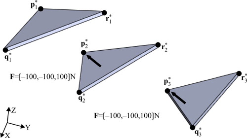
Table 2. Precision position coordinates.

Pos. #	${\mathbf{p}}^{\ast }$ [m]	${\mathbf{q}}^{\ast }$ [m]	${\mathbf{r}}^{\ast }$ [m]
1	−0.7500,−0.7500,−0.5000	0.2159,−1.0088,−0.5000	−0.5154, 0.1254, −0.0774
2	0.3750, 0.3750, 0.2500	1.3664, 0.5055, 0.2500	0.2476, 1.3429, 0.0336
3	1.5000, 1.5000, 1.0000	2.3660, 2.0000, 1.0000	1.2132, 1.9967, 0.1808

7.2. Example: precision positions 1–2

Here, an RSSR-SS linkage is synthesized to approximate precision positions 1–2 in Figure 6. Table 3 includes the initial values and calculated values for the RSSR-SS linkage dimensions. The initial values were not determined arbitrarily, but judiciously by graphically visualizing the precision positions in 3D space. By graphically visualizing the precision position in 3D space using Computer Aided Design (CAD) software, one can sketch spatial RSSR-SS linkages from which initial values are selected. Using this approach, the initial RSSR-SS dimension values for the optimization model are specified far more judiciously that they would by random guessing.

Table 3. Initial and calculated RSSR-SS linkage variable values.

variable	initial values	calculated values
a0	−3, −3, 3	−1.0140. −1.6574, 3.3824
a1	−3, −3, 3	−1.1595, −1.3124, 0.3007
$\mathbf{u}{}_{{\mathbf{a}}_0}$	−0.5, 0.5, 0.5	−0.8087, 0.5792, 0.1030
b0	5, −5, 5	2.2400, −1.6886, 2.3063
b1	1, −1, 1	0.7723, −1.8300, 0.3007
$\mathbf{u}{}_{{\mathbf{b}}_0}$	−0.5, 0.5, 0.5	−0.7956, 0.2126, 0.5672
c0	1, 5, 5	0.3312, 1.5657, 3.7417
c1	−1, 1, 1	−0.6903, 0.4384, 1.1459
θ1–2, φ1–2, γ1–2	−50°, −50°, 100°	−43.4329°,−71.9654°, 75.5734°
Number of Iterations: 239 Elapsed Time: 9262 s

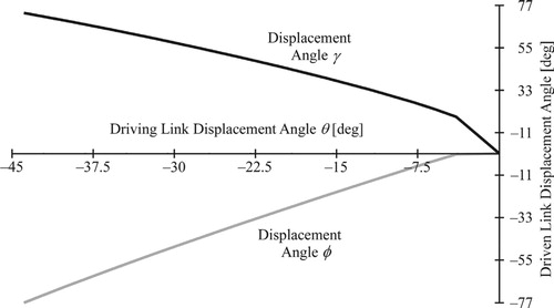
Table 4 includes the coupler positions achieved by the synthesized RSSR-SS motion generator (Figure 7). Figure 8 includes plots of displacement angles $\phi$ and $\gamma$ with respect to the crank displacement angle theta. As shown by the continuity of the displacement angle plots and the coupler positions achieved by the synthesized RSSR-SS motion generator, it is free of branch and circuit defects over the calculated driving link rotation range. While Inequality (29) ensures order-defect elimination, because order defects are not inherent in two-position synthesis problems (they occur in problems having at least three precision positions) this inequality is not required for this RSSR-SS optimization example. The driver torque required to achieve static equilibrium for the synthesized RSSR-SS linkage at coupler position 2 is 98N-m which is within the maximum specified magnitude of ${\tau }_{max}$.

Table 4. Coupler position coordinates achieved by the synthesized RSSR-SS linkage.

Pos. #	p [m]	q [m]	r [m]
1	−0.7500,−0.7500,−0.5000	0.2159, −1.0088,−0.5000	−0.5154, 0.1254, −0.0774
2	0.3777, 0.3781, 0.2484	1.3693, 0.5079, 0.2500	0.2514, 1.3464, 0.0330

Figure 7. Synthesized RSSR-SS linkage at (top) initial and (bottom) final achieved coupler positions.

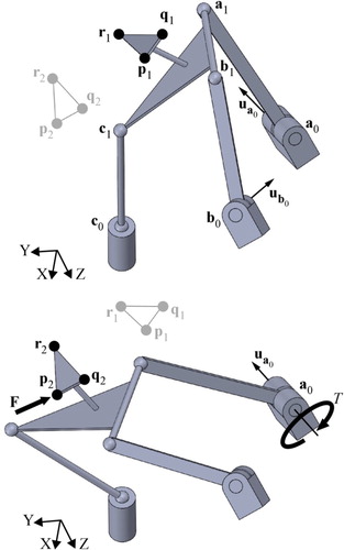
Figure 8. Driven link displacement angles (versus driving link rotation) for synthesized linkage.

7.3. Example: precision positions 1–3

Here, an RSSR-SS linkage is synthesized to approximate precision positions 1–3 in Figure 6. Table 5 includes the initial values and calculated values for the RSSR-SS linkage dimensions. Table 6 includes the coupler positions achieved by the synthesized RSSR-SS motion generator (Figure 9). Figure 10 includes plots of displacement angles $\phi$ and $\gamma$ with respect to the crank displacement angle theta. As shown by the continuity of the displacement angle plots and the coupler positions achieved by the synthesized RSSR-SS motion generator, it is free of branch and circuit defects over the calculated driving link rotation range. Being another two-position RSSR-SS optimization example (like the example in Section 7.2), Inequality (29) is not required. The driver torque required to achieve static equilibrium for the synthesized RSSR-SS linkage at coupler position 3 is −236N-m which is within the maximum specified magnitude of ${\tau }_{max}$.

Figure 9. Synthesized RSSR-SS linkage at (top) initial and (bottom) final achieved coupler positions.

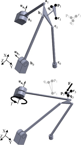
Figure 10. Driven link displacement angles (versus driving link rotation) for synthesized linkage.

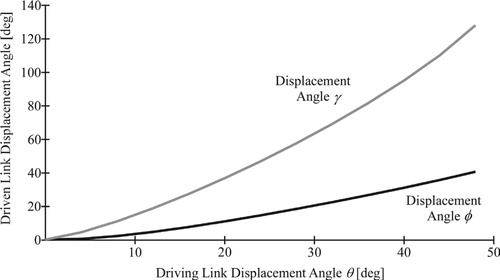
Table 5. Initial and calculated RSSR-SS linkage variable values.

variable	initial values	calculated values
a0	−3, −3, 3	3.6571, −1.8056, 6.2335
a1	4, −4, 1	0.7723, −1.8300, 0.3007
$\mathbf{u}{}_{{\mathbf{a}}_0}$	0.5, 0.5, 0.5	0.8781, −0.2178, −0.4261
b0	−2, 0.5, 2	−3.3603, 0.3239, 5.6743
b1	−5, −5, 0.5	−1.1595, −1.3124, 0.3007
$\mathbf{u}{}_{{\mathbf{b}}_0}$	0.5, 0.5, 0.5	0.6435, −0.6179, 0.4517
c0	−2, 2, 2	−0.0911,3.7265,5.7921
c1	−4, 4, 1	−0.6903, 0.4384, 1.1459
θ1–2, φ1–2, γ1–2	30°, 50°, 70°	47.9849°, 40.3923°, 127.6369°
Number of Iterations: 261 Elapsed Time: 10121 s

Table 6. Coupler position coordinates achieved by the synthesized RSSR-SS linkage.

Pos. #	p [m]	q [m]	r [m]
1	−0.7500,−0.7500,−0.5000	0.2159,−1.0088,−0.5000	−0.5154, 0.1254, −0.0774
3	1.5009, 1.5007, 1.0032	2.3671, 2.0004, 1.0028	1.2147, 1.9961, 0.1830

7.4. Applicability of optimum motion generation with static loading in engineering design

Kinematics (which includes motion generation) is only one of several engineering disciplines to consider in the design of linkage systems. Beyond a kinematic analysis, structural analyses where forces and deformations are accounted for are also considered. The RSSR-SS linkage solutions in Sections 7.2 and 7.3 have not only been synthesized to approximate prescribed coupler positions, but also to satisfy prescribed maximum driver torque values under prescribed coupler static loads. Therefore, when the driving links of both solutions are designed for example, one already knows the static torque capacity (${\tau }_{max}$) to apply to the driver in a finite element analysis (to analyze link stresses, strains and deflections) or in the selection of a drive system for the RSSR-SS linkage. Synthesizing the RSSR-SS linkage without considering static loads could result in repeated ‘trial and error’ attempts to synthesize a linkage that requires a suitable driver torque for a known RSSR-SS coupler force. So in summary, the inclusion of static loading in RSSR-SS dimensional synthesis makes the user more efficient in design of RSSR-SS linkages when static structural loading is to be considered in linkage design.

8. Discussion

While the authors presented RSSR-SS synthesis examples where all of the linkage dimensions are included among the variables to be calculated, the user is free to exclude any dimension from among the variables and prescribe them instead (e.g. fixed pivots ${\mathbf{a}}_0$, ${\mathbf{b}}_0$ and ${\mathbf{c}}_0$). Any excluded dimension will eliminate their corresponding partial derivatives in the gradients and Hessians of the optimization model.

The particular computing platform used to develop and run the 2-position RSSR-SS optimization model was a 64-bit Windows laptop with 16 gigabytes of memory and a 2.1 GHz processor. The amount of memory required to run a constrained optimization model is largely dependent on the number of variables included in the model. While there are only 27 specific types of variables in the optimization model used in Section 5, these variables appear over 2.7 million times in Equations (15) through (28) (for N = 2) alone.

From Table 1, it can be observed that the largest equations include either the displaced moving pivot $\mathbf{c}$ from Equation (4) or the displaced coupler point $\mathbf{p}$ from Equation (5). Both equations include the coupler rotation matrix $\left[R_{\omega ,\mathbf{w}}\right]$ which includes the rotation axis vector $\mathbf{w}$ from Equation (6). The chief contributor to the sizes of Equations (15), (23) through (25) and Inequalities (27) and (28) is the inclusion of the rotation axis vector $\mathbf{w}$. If an alternate analytical kinematic RSSR-SS displacement model could be formulated that does not require this coupler rotation, then it is possible that a much smaller and subsequently more manageable RSSR-SS optimization model could be produced.

Another possible option is to consider an alternate solution algorithm. Evolutionary Algorithms are algorithms based on a natural selection process that mimics biological evolution. In the context of planar linkage motion generation, the evolutionary algorithm method has been noted to offer simplicity of implementation and fast convergence to the optimal solution with no need of a substantial knowledge of the solution space [14,15]. Perhaps the large-scale RSSR-SS optimization model would be a more manageable problem when solved using these algorithms.

Making the RSSR-SS optimization more practical on a personal computing platform would greatly expand the number of precision positions the user can define. Making the model more practical would also make the implementation of auxiliary design studies possible. For example, stochastic analysis methods enable the use of parameters with uncertainties in RSSR-SS design [16]. Rather than static loads, modal and distributed dynamic loads are also relevant conditions in real-word engineering design [17]. Incorporating analysis methods for boundary lubrication is also a relevant condition where journal bearings are considered (as the revolute joints) in RSSR-SS design [18].

9. Conclusion

A general RSSR-SS optimization model for defect-free motion generation with static loading was implemented in this work. With this model, both the dimensions of an RSSR-SS linkage required to approximate precision positions were calculated as well as the static driver torque for the linkage given a precision position force. Its primary drawbacks (in Matlab on a personal computer) are the large file sizes of the algebraic gradients and Hessians for the optimization model’s objective function and constraints. Only a 2-position RSSR-SS optimization model with partial user-supplied gradients and no Hessians could be produced and demonstrated in this work on a 64-bit laptop computer with 16 gigabytes of memory.

Disclosure statement

No potential conflict of interest was reported by the authors.

References

- Dasgupta B, Mruthyunjaya TS. The Stewart platform manipulator: A Review. Mech Mach Theory. 2000;35(1):15–40. doi: 10.1016/S0094-114X(99)00006-3
- Sandor GN, Xu LJ, Yang SP. Computer-Aided synthesis of Two-closed-loop RSSR-SS spatial motion generator with Branching and sequence constraints. Mech Mach Theory. 1986;21(4):345–350. doi: 10.1016/0094-114X(86)90056-X
- Russell K, Sodhi RS. Kinematic synthesis of adjustable RSSR-SS Mechanisms for multi-Phase finite and Multiply-Separated positions. ASME Journal of Mechanical Design. 2003a;125(4):847–853. doi: 10.1115/1.1631576
- Russell K, Sodhi RS. On displacement analysis of the RSSR-SS mechanism. Mech Based Des Struct Mach. 2003b;31(2):281–296. doi: 10.1081/SME-120020294
- Shen Q, Russell K, Sodhi RS. Analytical Displacement and Velocity Modeling of the RSSR-SS Linkage, Proceedings of the 11th International Conference on the Theory of Machines and Mechanisms, Liberec, Czech Republic (2012).
- Shen Q, Russell K, Sodhi RS, et al. Spherical four-Bar motion generation with a prescribed rigid-body Load. Transactions of the Canadian Society for Mechanical Engineering. 2008;32(3-4):401–410. doi: 10.1139/tcsme-2008-0026
- Russell K, Shen Q, Lee W, et al. On the synthesis of spatial RRSS motion Generators with prescribed coupler loads. JSME Journal of Advanced Mechanical Design, Systems and Manufacturing. 2009;3(3):236–244. doi: 10.1299/jamdsm.3.236
- Russell K, Shen Q. A general static torque constraint for spatial four-Bar motion generation with a coupler Load. ASME Journal of Mechanisms and Robotics. 2010;2(4):044502. doi: 10.1115/1.4002514
- Russell K, Shen Q, Lee W, et al. On the synthesis of spatial Revolute-Revolute-Spherical-Cylindrical motion Generators with prescribed coupler loads. Journal of Multi-Body Dynamics. 2010;224(2):183–190.
- Balli SS, Chand S. Defects in link Mechanisms and solution Rectification. Mech Mach Theory. 2002;37(9):851–876. doi: 10.1016/S0094-114X(02)00035-6
- Mallik AK, Ghosh A, Dittrich D. Kinematic analysis and synthesis of Mechanisms. Boca Raton: CRC Press; 1994.
- de Jalón J G. Twenty-five Years of natural coordinates. Multibody Syst Dyn. 2007;18(1):15–33. doi: 10.1007/s11044-007-9068-0
- Constrained Nonlinear Optimization Algorithms. Available from: https://www.mathworks.com/help/optim/ug/constrained-nonlinear-optimization-algorithms.html (Accessed on: January 14, 2019).
- Acharyya SK, Mandal M. Performance of EAs for four-Bar linkage synthesis. Mech Mach Theory. 2009;44(9):1784–1794. doi: 10.1016/j.mechmachtheory.2009.03.003
- Cabrera JA, Simon A, Prado M. Optimal synthesis of Mechanisms with Genetic algorithms. Mech Mach Theory. 2002;37(10):1165–1177. doi: 10.1016/S0094-114X(02)00051-4
- Liun J, Hu Y, Xu C, et al. Probability Assessments of Identified parameters for stochastic Structures using point estimation method. Reliability Engineering and System Safety. 2016;156:51–58. doi: 10.1016/j.ress.2016.07.021
- Li K, Liu J, Han X, et al. Distributed dynamic Load Identification based on Shape function method and Polynomial selection Technique. Inverse Probl Sci Eng. 2017;25(9):1323–1342. doi: 10.1080/17415977.2016.1255740
- Li K, Liu J, Han X, et al. Identification of Oil-film Coefficients for a Rotor-journal Bearing system based on Equivalent Load Reconstruction. Tribol Int. 2016;104:285–293. doi: 10.1016/j.triboint.2016.09.012