Use of moving average filter for regularization of the transfer function based on Green's function method (TFBGF) to solve an IHCP

ABSTRACT

Most techniques for inverse problems minimize the least squares error function between the calculated and measured temperature to estimate the heat flux in the IHCP. In this work, we apply the method of the transfer function based on Green's functions (TFBGF). Unlike the optimization techniques, TFBGF is a technique that uses deconvolution of the measured temperature and the heat transfer function of the system to estimate the unknown heat flux in a forward way.However, due to the presence of the inherent experimental uncertainties, some regularization methods may be necessary to add stability to the inverse solution. The regularization procedure proposed here is the moving average filters. Since the convolution has a filter characteristic, it has the advantage of being able to be implemented easily and incorporated to TFBGF method. In this work, an experimental procedure is designed to demonstrate the ability and technical robustness of TFBGF method with the regularization considering temperature data in regions of low sensitivity and high experimental uncertainty.

KEYWORDS:

• Heat transfer function
• Green's function
• moving average filter
• IHCP

2010 MATHEMATICS SUBJECT CLASSIFICATION:

• 15A29

1. Introduction

Inverse heat conduction problems (IHCP) belong to the class of problems called mathematically ill-posed. In opposition, well-posed problems require (i) existence, (ii) uniqueness and (iii) stability of the solution. It is proved in [1] that the solution of an inverse problem in heat conduction obtained by means of differential equations is usually difficult because it does not satisfy the condition of stability. This problem is caused by the noise present in measured temperatures. The stability condition is correlated to the continuous dependence of the data, thus, small oscillations in temperature can cause large discrepancies in the estimation of heat flux.

The classical methods of solving inverse problems in conduction are usually based on minimizing the sum of the squares of the differences between the experimental and the calculated temperatures which in turn is a function of the heat flux which is intended to be estimated [2]. Thus, to reach the success in the estimation of the heat flux these methods provide mechanisms that look by stability of the solution.

For example, based on the least squares method and Duhamel theorem, Beck et al. [1] developed the sequential function specification method (SFSM), which is still one of the most used techniques for solving inverse heat conduction problems and is widely used for estimating heat flux either constant or linear forms. The technique consists of successive minimization of the error estimated for the current time and some future time steps. In the sequential function specified method the future time is responsible for ensuring stability to the solution of the inverse problem [1]. The classical SFSM is reviewed by Samadi et al. and a general framework is developed for solving inverse heat conduction problem using SFSM with hypothesis of polynomials functions. A generalized algorithm is used to define polynomials of any degree and estimate heat fluxes using SFSM with any number of past and future data [3].

Some researchers have proposed adaptations of this method seeking minimization of problems arising from the existence of measurement errors [4]. The objective is to obtain greater stability of the algorithm. In this case, Keanini et al. [4] proposed a modified method of the sequential function specification method to stabilize the inverse parabolic problem of heat conduction. The method uses computational time steps which are larger than the experimental sampling intervals as well as the future time steps that are equal to the sampling intervals.

Regularization is another artifice used to convert mathematically ill-conditioned problems into well-conditioned problems. Tikhonov regularization technique is widely used to ensure stability to the IHCP. In this method, one or more terms have been added to the sum of the least squares. The authors in [5] concludes in their work that Tikhonov regularization can be interpreted as a digital filter for real-time data processing.

The relationship between the thermal response and the unknown input can be expressed through a sensitivity matrix. The sensitivity matrix tends to be quasi-singular. Another effective technique to solve ill-posed problems is based in the Singular Value Decomposition (SVD) of an ill-conditioned matrix [6–8].

The proper orthogonal decomposition (POD) method is investigated in [7]. This method is based on the dynamics of the problem in studied, that can be solved by two approaches. In the first way the governing PDE is reduced to a system of ODE's which reduces the computational time considerably. In the second approach the ill-conditioned matrix is modified using the singular value decomposition (SVD) which reduces the destructive effects of the random noise of the temperature data.

Another technique often used is the conjugate gradient method with adjoint equation described in detail in [9,10]. This technique is based on an optimization process using iterative regularization, that is, the results of minimization of the objective function tend to stabilize through iterations.

Ahmadi et al. presented an efficient application of wavelets as a strategy to remove the effect of noise on inverse heat conduction problems solved by the variable metric method [11]. Farahani et al. compared mollification, transformed wavelets and moving average methods as alternatives to minimize the effect of noise inherent to the experimental measures [12]. In the comparison of these techniques, the insertion of the mollification method as a step prior to the application of the conjugate gradient and Tikhonov regularization methods showed smaller variance error for the estimation of the heat flux.

This work evaluates the application of the moving average filter in conjunction with the TFBFG method, whose objective is to convert poorly conditioned problems into an approximate well-conditioned problems. In the TFBFG method the solution of the inverse problem identifies the analytical transfer function by means of Green's functions. It is a simple approach without iterative processes, and therefore extremely fast. As the technique uses the principle of linear superposition and deconvolution, any noise due to errors in temperature measurement is directly transported and amplified for the estimated heat flux components. The TFBGF method is described in detail in [13] with application in thermal problems related to the orthogonal machining process with success for higher temperature gradient. If the temperature is high and the noise is low, that is, noise is not significant, the problem behaves as a well-conditioned problem. In this case, heat flow can be estimated directly without the use of the moving average. The analysis of the moving average filter in this research is presented through simulated and experimental tests for lower temperature gradient.

2. Transfer function based on Green's function method (TFBGF)

The TFBGF method for IHCP depends essentially on the identification of the transfer function, which in turn is obtained from the Green's function that provides the solution of the direct heat conduction problem. The Green's functions for heat conduction problems are readily available in [14]. TFBGF is a proposed solution of inverse problem that can be applied to the various physical phenomena described by linear differential equations, and in this research the objective is to estimate heat flux.

The transfer function is responsible for characterizing the relationship between input and output of a dynamic system. In this case, the heat flux, $q\left(t\right)$, is the input of the system (excitation) and the temperature, $T(\mathbf{x},t)$, is the response (cause) to that excitation, as shown by the block diagram (Figure 1).

Figure 1. Block diagram of a one input/one output dynamic system.

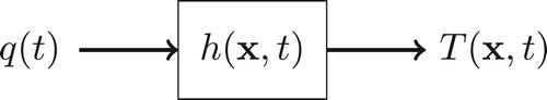
In the time domain the relation between input/output is given by the convolution, i.e. (1) $T(\mathbf{x},t)=h(\mathbf{x},t)\ast q\left(t\right).$(1) In the complex domain, with the s variable, the analysis of dynamic systems is facilitated due to the use of the Laplace transform, thus, the input/output relation is given by multiplication, (2) $T(\mathbf{x},s)=H(\mathbf{x},s).q\left(s\right),$(2) where the transfer function is given by $H(\mathbf{x},s)=\mathcal{L}\left\{h\right(\mathbf{x},t\left)\right\}$.

Or again, returning to the time domain, through the inverse transform of Laplace, we have, (3) $\begin{array}{rl}T(\mathbf{x},t)& ={\mathcal{L}}^{-1}\left\{H\right(\mathbf{x},s).q(s\left)\right\}\\ & =h(\mathbf{x},t)\ast q\left(t\right)={\int }_0^{t}h(\mathbf{x},t-\tau )q\left(\tau \right)\mathrm{d}\tau .\end{array}$(3) It is observed that the transfer function is a property of the system, therefore, it is independent of the input/output pair of the dynamic system. Thus, by considering the heat flux as the Dirac Delta function, $q\left(t\right)=\delta \left(t\right)$, the temperature, $T(x,t)$, is the so-called impulse response function of the system. The transfer function can be defined as the Laplace transform of the impulse response function, i.e. $H(\mathbf{x},s)=\mathcal{L}\left\{h\right(\mathbf{x},t\left)\right\}$, where $h(\mathbf{x},t)$ is the impulse response function.

From the property of the neutral element¹ of convolution we have that $T(\mathbf{x},t)=h(\mathbf{x},t)\ast \delta \left(t\right)=h(\mathbf{x},t)$, this means that the system's impulse response function is given by the temperature field when the excitation is a Dirac Delta type pulse. Therefore, if the thermal problem can be modelled analytically by means of the Green's functions, then the impulse response is immediately identified.

According to [15], the convolution procedure between the input of the system and its impulse response function (IRF) is the most rigorous way to implement a digital filter. In this case, the filter is called a kernel. In dynamic systems there are three study variables: the excitation (heat flux), the transfer function and the system response (temperature), in this way the problems are solved knowing always two variables and estimating the third. Thus, by knowing the experimental temperatures and the impulse response (transfer function), the estimation for the heat flux in the TFBGF method can be accomplished by different approaches, by means of the deconvolution concept, or by applying the fast Fourier transform and its inverse, or else, by the spectral density calculus, all equivalent to each other [13].

At the core of the TFBG method is to identify the impulse response function of the thermal problem, in the Section 4.2 it is shown how the impulse response is obtained considering a three-dimensional problem in Cartesian coordinates, which is object of study for this research.

By using the relations between input/output of a dynamic system, in the complex domain s (Equation (2(2) $T(\mathbf{x},s)=H(\mathbf{x},s).q\left(s\right),$(2) )), the heat flux, $q\left(s\right)$, is estimated by (4) $q\left(s\right)=T(\mathbf{x},s)/H(\mathbf{x},s).$(4) Applying the inverse Laplace transform on $q\left(s\right)$ gives $q\left(t\right)$ as (5) $q\left(t\right)={\mathcal{L}}^{-1}\left\{q\right(s\left)\right\}.$(5) Alternatively one can obtain $q\left(t\right)$ by deconvolution (6) $q\left(t\right)=T(\mathbf{x},t)\ast {\mathcal{L}}^{-1}\left\{1/H\right(\mathbf{x},s\left)\right\}.$(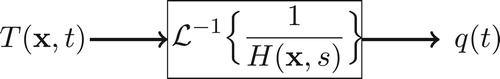6) Thus, the block diagram representation for inverse problem, given by Equations (4(4) $q\left(s\right)=T(\mathbf{x},s)/H(\mathbf{x},s).$(4) ) and (6(6) $q\left(t\right)=T(\mathbf{x},t)\ast {\mathcal{L}}^{-1}\left\{1/H\right(\mathbf{x},s\left)\right\}.$(6) ), is shown in Figure 2. We observe the inversion of the input/output pair and that the system is described by ${\mathcal{L}}^{-1}\left\{1/H\right(\mathbf{x},s\left)\right\}$.

Figure 2. Block diagram of the dynamic system for the inverse problem.

However, it is found that the presence of noise, $\epsilon \left(t\right)$, in the measured temperature can cause great discrepancies in the estimate of the heat flux, that is, considering (7) $T(\mathbf{x},t)\pm \epsilon \left(t\right)=q\left(t\right)\ast h(\mathbf{x},t),$(7) then, by applying the Laplace transform, we have (8) $\mathcal{L}\left\{T\right(\mathbf{x},t)\pm \epsilon (t\left)\right\}=\mathcal{L}\left\{q\right(t)\ast h(\mathbf{x},t\left)\right\},$(8) this is, (9) $T(\mathbf{x},s)\pm \epsilon \left(s\right)=q\left(s\right)\cdot H(\mathbf{x},s)$(9) therefore, (10) $q\left(s\right)=\frac{T(\mathbf{x},s)}{H(\mathbf{x},s)}\pm \frac{\epsilon \left(s\right)}{H(\mathbf{x},s)}.$(10) Applying the inverse Laplace transform, we have (11) $q\left(t\right)={\mathcal{L}}^{-1}\left\{\frac{T(\mathbf{x},s)}{H(\mathbf{x},s)}\right\}\pm {\mathcal{L}}^{-1}\left\{\frac{\epsilon \left(s\right)}{H(\mathbf{x},s)}\right\},$(11) or, in terms of convolution, (12) $q\left(t\right)=T(\mathbf{x},t)\ast {\mathcal{L}}^{-1}\left\{\frac{1}{H(\mathbf{x},s)}\right\}\pm \epsilon \left(t\right)\ast {\mathcal{L}}^{-1}\left\{\frac{1}{H(\mathbf{x},s)}\right\}.$(12) It is observed in the last term of Equation (12(12) $q\left(t\right)=T(\mathbf{x},t)\ast {\mathcal{L}}^{-1}\left\{\frac{1}{H(\mathbf{x},s)}\right\}\pm \epsilon \left(t\right)\ast {\mathcal{L}}^{-1}\left\{\frac{1}{H(\mathbf{x},s)}\right\}.$(12) ) that the presence of significant noises in the temperature is responsible for causing discrepancies in the estimate of the heat flux. If noise is significant, the ill-condition of the problem is provided by that term, so it becomes necessary to minimize the effect of noise. Thus, the purpose of applying the moving average filter is to minimize the noise from the use of the experimental temperature, i.e. in the Equations (7(7) $T(\mathbf{x},t)\pm \epsilon \left(t\right)=q\left(t\right)\ast h(\mathbf{x},t),$(7) )–(12(12) $q\left(t\right)=T(\mathbf{x},t)\ast {\mathcal{L}}^{-1}\left\{\frac{1}{H(\mathbf{x},s)}\right\}\pm \epsilon \left(t\right)\ast {\mathcal{L}}^{-1}\left\{\frac{1}{H(\mathbf{x},s)}\right\}.$(12) ), make $\epsilon \left(t\right)$ tend to zero.

In Equation (7(7) $T(\mathbf{x},t)\pm \epsilon \left(t\right)=q\left(t\right)\ast h(\mathbf{x},t),$(7) ), represented by the block diagram in Figure 3, it is possible to observe that the noise present at the temperature is transferred to the heat flux, and, is modulated as $\delta \left(t\right)=\epsilon \left(t\right)\ast {\mathcal{L}}^{-1}\left\{1/H\right(\mathbf{x},s\left)\right\}$ tends to zero.

Figure 3. Block diagram for the inverse problem with temperature noise.

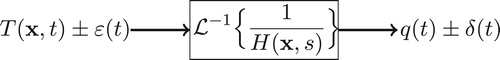
In this way, moving average filter can be applied either a priori (in temperature) or a posteriori (in the heat flow), or even simultaneously. The option to apply the moving average as a filter is due to the ease of implementation of the algorithm, its low computational cost and its efficiency.

3. Moving average filter

The simple moving average is a digital filter of easy understanding and use, and therefore, of wide application. Despite its mathematical simplicity, the moving average is ideal for the reduction of random noise present in experimental data. This procedure is equivalent to a low pass filter [12].

Smith [15] describes the moving average filter by averaging the number of points from the input signal to each point in the output signal, Equation (13(13) $y\left[i\right]=\frac{1}{n}\sum _{j=0}^{n-1}x[i+j],$(13) ). It is noted that moving average filter is a convolution of the signal with a rectangular pulse having an area of one. (13) $y\left[i\right]=\frac{1}{n}\sum _{j=0}^{n-1}x[i+j],$(13) where $x\left[i\right]$ is the input data and $y\left[i\right]$ is the input data smoothing by replacing each $x\left[i\right]$ with the mean of consecutive n data.

In the Figure 4 the effect of ‘smoothing’ on the temperature data is observed when the average is applied, considering $n=10,50\mathrm{a}\mathrm{n}\mathrm{d}100$. In this example we considered the addition of a random error of $\pm {0.15}^{\circ }$C, which corresponds to 1% of the maximum value of the simulated temperature. It is observed that for $n=10$ the data was smoothed around average values of the curve if adjusted the tendency of the curve. However, for $n=50$ and $n=100$, smoothed data escaped the original evolution, implying that there is an optimal number of n that establishes a compromise between noise smoothing without altering the original behaviour of data.

Figure 4. Effect of moving average ($n=10,50\mathrm{a}\mathrm{n}\mathrm{d}100$) on simulated temperature with error ($\epsilon =\pm 0.15$) of $1\mathrm{\%}$ of maximum value.

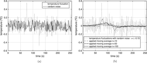
The effect of the moving average can also be exploited by comparing temperature fluctuation data $\left(T\right(t_i)-T(t_{i+1}\left)\right)$ with random noise, evidently for simulated data studies. In Figure 5(a), a comparison of these signals is performed, while in Figure 5(b), the results for reduction of temperature fluctuation after applying the moving average is shown. It is observed that the larger the value of n, the lower the data fluctuation, however, in the case of n=100 the smoothing occurs so drastically that it compromises the behaviour of the temperature data, as already noted in Figure 4.

Figure 5. Minimization of temperature fluctuation using moving average. (a) Random noise Vs temperature fluctuation. (b) Temperature fluctuation with moving average ($n=10,50,\mathrm{a}\mathrm{n}\mathrm{d}100$).

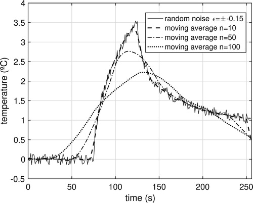
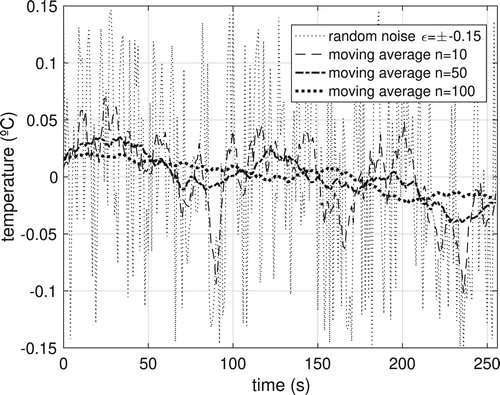
Therefore, the value of n should be chosen so that noise minimization is enough to transform the problem from a poorly conditioned into an approximate well-conditioned one, without changing the behaviour of the curve. According to [15], of all possible linear filters, the moving average produces the best noise minimization that does not imply in changing the behaviour of the curve. The noise reduction is proportional to the square root of the number of points of the mean, that is, if n=10, then the noise will be reduced to the factor of $\sqrt{10}$. Therefore, if the noise considered is $\epsilon =\pm 0.15$, then, after the application of the moving average, the residual noise is given by ${\epsilon }_r=\frac{\pm 0.15}{\sqrt{10}}\approx \pm 0.0474$. In Figure 6 it is possible to observe the noise reduction factor for n=10,50 and 100.

Figure 6. Effect of moving average on simulated noise.

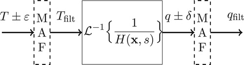
It can be observed that the moving average filter can be applied both in the experimental data (measured temperature) and in the estimated values (heat flux), by means of the Equations (7(7) $T(\mathbf{x},t)\pm \epsilon \left(t\right)=q\left(t\right)\ast h(\mathbf{x},t),$(7) ) and (12(12) $q\left(t\right)=T(\mathbf{x},t)\ast {\mathcal{L}}^{-1}\left\{\frac{1}{H(\mathbf{x},s)}\right\}\pm \epsilon \left(t\right)\ast {\mathcal{L}}^{-1}\left\{\frac{1}{H(\mathbf{x},s)}\right\}.$(12) ) or simultaneously. The block diagram presented in Figure 7 contemplates the possible applications of the moving average filter in conjunction with the TFBGF technique.

Figure 7. Moving average filter (MAF) applied to TFBGF.

4. Mathematical model

We present in this section the mathematical model for the thermal problem used for the analysis of the application of the moving average in the estimation of the heat flux of an IHCP using TFBGF. The transient and three-dimensional thermal model, shown in Figure 8, called $X23Y23Z23$ by [14] investigated in this paper corresponds to the experimental apparatus shown in Section 5.

Figure 8. Tridimensional thermal model (X23Y23Z23).

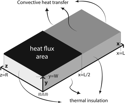
The thermal problem $X23Y23Z23$ refers to a rectangular geometry whose boundary conditions in the directions x, y and z are given by the boundary conditions of type 2, prescribed heat flux, and boundary condition of type 3, surface exposed to heat convection [14]. For the planes xy, yz and xz that intersect at the origin, zero heat flux is imposed. It is observed in Figure 8 that in x=L and z=R the surfaces are exposed to the convective medium and the heat flux, $q\left(t\right)$, is imposed on area highlighted in y=W, with the remaining area exposed to the convective medium.

The governing equation of the thermal problem represented in Figure 8 is given by (14a) $\frac{{\mathrm{\partial }}^2\theta }{\mathrm{\partial }{x}^2}+\frac{{\mathrm{\partial }}^2\theta }{\mathrm{\partial }{y}^2}+\frac{{\mathrm{\partial }}^2\theta }{\mathrm{\partial }{z}^2}=\frac{1}{\alpha }\frac{\mathrm{\partial }\theta }{\mathrm{\partial }t}$(14a) subjected to boundary conditions to $t\in (0,\mathrm{\infty })$: (14b) $\begin{array}{rl}& {\left.-k\frac{\mathrm{\partial }\theta }{\mathrm{\partial }x}\right|}_{x=0}=0,{\left.-k\frac{\mathrm{\partial }\theta }{\mathrm{\partial }y}\right|}_{y=0}=0,{\left.-k\frac{\mathrm{\partial }\theta }{\mathrm{\partial }z}\right|}_{z=0}=0,\\ & {\left.-k\frac{\mathrm{\partial }\theta }{\mathrm{\partial }x}\right|}_{x=L}=h\theta ,{\left.-k\frac{\mathrm{\partial }\theta }{\mathrm{\partial }z}\right|}_{z=R}=h\theta ,\\ & {\left.-k\frac{\mathrm{\partial }\theta }{\mathrm{\partial }y}\right|}_{y=W}=h\theta -q\left(t\right),\\ & q\left(t\right)\in \left(0,\frac{L}{2}\right)\times (0,R);h\theta \in \left(\frac{L}{2},L\right)\times (0,R)\end{array}$(14b) and the initial condition: (14c) $\begin{array}{rl}& {\theta }_0=T(x,y,z,0)-T_{\mathrm{\infty }},\\ & (x,y,z)\in (0,L)\times (0,W)\times (0,R),\end{array}$(14c) where $\theta =T-T_{\mathrm{\infty }}$, where T is the temperature of the body and $T_{\mathrm{\infty }}$ is the temperature of the medium, k and h are, respectively, the thermal diffusivity, the thermal conductivity and the coefficient of heat exchange by convection.

Equations (14a(14a) $\frac{{\mathrm{\partial }}^2\theta }{\mathrm{\partial }{x}^2}+\frac{{\mathrm{\partial }}^2\theta }{\mathrm{\partial }{y}^2}+\frac{{\mathrm{\partial }}^2\theta }{\mathrm{\partial }{z}^2}=\frac{1}{\alpha }\frac{\mathrm{\partial }\theta }{\mathrm{\partial }t}$(14a) )–(14c(14c) $\begin{array}{rl}& {\theta }_0=T(x,y,z,0)-T_{\mathrm{\infty }},\\ & (x,y,z)\in (0,L)\times (0,W)\times (0,R),\end{array}$(14c) ) represent the thermal model of the direct problem studied. If the heat flux $q\left(t\right)$ is an unknown function and a variable to be estimated, then the inverse problem is established. The solution to the direct problem is presented below. Details of the solution to this problem can be found in the work of [1,13].

4.1. Direct problem: solution by Green's functions

The solution of the problem described by Equations (14a(14a) $\frac{{\mathrm{\partial }}^2\theta }{\mathrm{\partial }{x}^2}+\frac{{\mathrm{\partial }}^2\theta }{\mathrm{\partial }{y}^2}+\frac{{\mathrm{\partial }}^2\theta }{\mathrm{\partial }{z}^2}=\frac{1}{\alpha }\frac{\mathrm{\partial }\theta }{\mathrm{\partial }t}$(14a) )–(14c(14c) $\begin{array}{rl}& {\theta }_0=T(x,y,z,0)-T_{\mathrm{\infty }},\\ & (x,y,z)\in (0,L)\times (0,W)\times (0,R),\end{array}$(14c) ) in terms of Green's functions is given by (15) $\begin{array}{rl}& \theta (x,y,z,t)\\ & ={\int }_{x^{\prime }=0}^L{\int }_{y^{\prime }=0}^W{\int }_{z^{\prime }=0}^{R}G(x,y,z,t|x^{\prime },y^{\prime },z^{\prime },0){\theta }_0\mathrm{d}{x}^{\prime }\mathrm{d}{y}^{\prime }\mathrm{d}{z}^{\prime }\\ & +\frac{\alpha }{k}{\int }_{\tau =0}^t{\int }_{x^{\prime }=0}^{L/2}{\int }_{z^{\prime }=0}^{R}q\left(\tau \right)G(x,y,z,t|x^{\prime },W,z^{\prime },\tau )\mathrm{d}{x}^{\prime }\mathrm{d}{z}^{\prime }\mathrm{d}\tau .\end{array}$(15) The Green's function for the problem given by the Equation (15(15) $\begin{array}{rl}& \theta (x,y,z,t)\\ & ={\int }_{x^{\prime }=0}^L{\int }_{y^{\prime }=0}^W{\int }_{z^{\prime }=0}^{R}G(x,y,z,t|x^{\prime },y^{\prime },z^{\prime },0){\theta }_0\mathrm{d}{x}^{\prime }\mathrm{d}{y}^{\prime }\mathrm{d}{z}^{\prime }\\ & +\frac{\alpha }{k}{\int }_{\tau =0}^t{\int }_{x^{\prime }=0}^{L/2}{\int }_{z^{\prime }=0}^{R}q\left(\tau \right)G(x,y,z,t|x^{\prime },W,z^{\prime },\tau )\mathrm{d}{x}^{\prime }\mathrm{d}{z}^{\prime }\mathrm{d}\tau .\end{array}$(15) ) is given by [14] (16) $\begin{array}{rl}& G(x,y,z,t|x^{\prime },y^{\prime },z^{\prime },\tau )\\ & =\frac{8}{LWR}\sum _{p=1}^{\mathrm{\infty }}\sum _{n=1}^{\mathrm{\infty }}\sum _{m=1}^{\mathrm{\infty }}{\mathrm{e}}^{-\left(\frac{{\alpha }_m^2}{L^2}+\frac{{\beta }_n^2}{W^2}+\frac{{\gamma }_p^2}{R^2}\right)\alpha (t-\tau )}\\ & \times \left[\frac{{\alpha }_m^2+B_1^2}{{\alpha }_m^2+B_1^2+B_1}\right]\left[\frac{{\beta }_n^2+B_2^2}{{\beta }_n^2+B_2^2+B_2}\right]\left[\frac{{\gamma }_p^2+B_3^2}{{\gamma }_p^2+B_3^2+B_3}\right]\\ & \times \left[\cos \left(\frac{{\alpha }_{m}x}{L}\right)\cos \left(\frac{{\alpha }_m{x}^{\prime }}{L}\right)\right]\left[\cos \left(\frac{{\beta }_{n}y}{W}\right)\cos \left(\frac{{\beta }_n{y}^{\prime }}{W}\right)\right]\\ & \times \left[\cos \left(\frac{{\gamma }_{p}z}{R}\right)\cos \left(\frac{{\gamma }_p{z}^{\prime }}{R}\right)\right]\end{array}$(16) where ${\alpha }_m$, ${\beta }_n$ and ${\gamma }_p$ are the eigenvalues by means of the transcendental equations ${\alpha }_m\tan {\alpha }_m=B_1$, ${\beta }_n\tan {\beta }_n=B_2$ and ${\gamma }_p\tan {\gamma }_p=B_3$. The indices $m=1,\dots ,M$, $n=1,\dots ,N$ and $p=1,\dots ,P$ define the amount of (iterations) required for the convergence of series, given a truncation error, ε, desired. Since $B_1=\frac{hL}{k}$, $B_2=\frac{hW}{k}$ and $B_3=\frac{hR}{k}$ are numbers associated with each surface.

Thus, by replacing the Green's function, Equation (16(16) $\begin{array}{rl}& G(x,y,z,t|x^{\prime },y^{\prime },z^{\prime },\tau )\\ & =\frac{8}{LWR}\sum _{p=1}^{\mathrm{\infty }}\sum _{n=1}^{\mathrm{\infty }}\sum _{m=1}^{\mathrm{\infty }}{\mathrm{e}}^{-\left(\frac{{\alpha }_m^2}{L^2}+\frac{{\beta }_n^2}{W^2}+\frac{{\gamma }_p^2}{R^2}\right)\alpha (t-\tau )}\\ & \times \left[\frac{{\alpha }_m^2+B_1^2}{{\alpha }_m^2+B_1^2+B_1}\right]\left[\frac{{\beta }_n^2+B_2^2}{{\beta }_n^2+B_2^2+B_2}\right]\left[\frac{{\gamma }_p^2+B_3^2}{{\gamma }_p^2+B_3^2+B_3}\right]\\ & \times \left[\cos \left(\frac{{\alpha }_{m}x}{L}\right)\cos \left(\frac{{\alpha }_m{x}^{\prime }}{L}\right)\right]\left[\cos \left(\frac{{\beta }_{n}y}{W}\right)\cos \left(\frac{{\beta }_n{y}^{\prime }}{W}\right)\right]\\ & \times \left[\cos \left(\frac{{\gamma }_{p}z}{R}\right)\cos \left(\frac{{\gamma }_p{z}^{\prime }}{R}\right)\right]\end{array}$(16) ), in Equation (15(15) $\begin{array}{rl}& \theta (x,y,z,t)\\ & ={\int }_{x^{\prime }=0}^L{\int }_{y^{\prime }=0}^W{\int }_{z^{\prime }=0}^{R}G(x,y,z,t|x^{\prime },y^{\prime },z^{\prime },0){\theta }_0\mathrm{d}{x}^{\prime }\mathrm{d}{y}^{\prime }\mathrm{d}{z}^{\prime }\\ & +\frac{\alpha }{k}{\int }_{\tau =0}^t{\int }_{x^{\prime }=0}^{L/2}{\int }_{z^{\prime }=0}^{R}q\left(\tau \right)G(x,y,z,t|x^{\prime },W,z^{\prime },\tau )\mathrm{d}{x}^{\prime }\mathrm{d}{z}^{\prime }\mathrm{d}\tau .\end{array}$(15) ), the analytical solution in terms of the variable θ is given by (17) $\begin{array}{rl}\theta (x,y,z,t)& =8{\theta }_0\sum _{p=1}^{\mathrm{\infty }}\sum _{m=1}^{\mathrm{\infty }}\sum _{n=1}^{\mathrm{\infty }}{\mathrm{e}}^{-\left(\frac{{\alpha }_m^2}{L^2}+\frac{{\beta }_n^2}{W^2}+\frac{{\gamma }_p^2}{R^2}\right)\alpha t}\\ & \times \left[\frac{{\alpha }_m^2+B_1^2}{{\alpha }_m^2+B_1^2+B_1}\right]\left[\frac{{\beta }_n^2+B_2^2}{{\beta }_n^2+B_2^2+B_2}\right]\left[\frac{{\gamma }_p^2+B_3^2}{{\gamma }_p^2+B_3^2+B_3}\right]\\ & \times \left[\cos \left(\frac{{\alpha }_{m}x}{L}\right)\frac{\sin {\alpha }_m}{{\alpha }_m}\right]\left[\cos \left(\frac{{\beta }_{n}y}{W}\right)\frac{\sin {\beta }_n}{{\beta }_n}\right]\\ & \times \left[\cos \left(\frac{{\gamma }_{p}z}{R}\right)\frac{\sin {\gamma }_p}{{\gamma }_p}\right]\\ & +\frac{8\alpha }{kW}\sum _{p=1}^{\mathrm{\infty }}\sum _{n=1}^{\mathrm{\infty }}\sum _{m=1}^{\mathrm{\infty }}{\mathrm{e}}^{-\left(\frac{{\alpha }_m^2}{L^2}+\frac{{\beta }_n^2}{W^2}+\frac{{\gamma }_p^2}{R^2}\right)\alpha t}\\ & \times \left[\frac{{\alpha }_m^2+B_1^2}{{\alpha }_m^2+B_1^2+B_1}\right]\left[\frac{{\beta }_n^2+B_2^2}{{\beta }_n^2+B_2^2+B_2}\right]\left[\frac{{\gamma }_p^2+B_3^2}{{\gamma }_p^2+B_3^2+B_3}\right]\\ & \times \left[\cos \left(\frac{{\alpha }_{m}x}{L}\right)\frac{\sin \left(\frac{{\alpha }_m}{2}\right)}{{\alpha }_m}\right]\left[\cos \left(\frac{{\beta }_{n}y}{W}\right)\cos {\beta }_n\right]\\ & \times \left[\cos \left(\frac{{\gamma }_{p}z}{R}\right)\frac{\sin \left(\frac{{\gamma }_p}{2}\right)}{{\gamma }_p}\right]{\int }_0^t\left[q\left(\tau \right){\mathrm{e}}^{\left(\frac{{\alpha }_m^2}{L^2}+\frac{{\beta }_n^2}{W^2}+\frac{{\gamma }_p^2}{R^2}\right)\alpha \tau }\right]\mathrm{d}\tau .\end{array}$(17) The solution in terms of the original variable T is readily obtained by $T=\theta +T_{\mathrm{\infty }}$. It is observed that the solution of the direct heat conduction problem $X23Y23Z23$ (Equation (17(17) $\begin{array}{rl}\theta (x,y,z,t)& =8{\theta }_0\sum _{p=1}^{\mathrm{\infty }}\sum _{m=1}^{\mathrm{\infty }}\sum _{n=1}^{\mathrm{\infty }}{\mathrm{e}}^{-\left(\frac{{\alpha }_m^2}{L^2}+\frac{{\beta }_n^2}{W^2}+\frac{{\gamma }_p^2}{R^2}\right)\alpha t}\\ & \times \left[\frac{{\alpha }_m^2+B_1^2}{{\alpha }_m^2+B_1^2+B_1}\right]\left[\frac{{\beta }_n^2+B_2^2}{{\beta }_n^2+B_2^2+B_2}\right]\left[\frac{{\gamma }_p^2+B_3^2}{{\gamma }_p^2+B_3^2+B_3}\right]\\ & \times \left[\cos \left(\frac{{\alpha }_{m}x}{L}\right)\frac{\sin {\alpha }_m}{{\alpha }_m}\right]\left[\cos \left(\frac{{\beta }_{n}y}{W}\right)\frac{\sin {\beta }_n}{{\beta }_n}\right]\\ & \times \left[\cos \left(\frac{{\gamma }_{p}z}{R}\right)\frac{\sin {\gamma }_p}{{\gamma }_p}\right]\\ & +\frac{8\alpha }{kW}\sum _{p=1}^{\mathrm{\infty }}\sum _{n=1}^{\mathrm{\infty }}\sum _{m=1}^{\mathrm{\infty }}{\mathrm{e}}^{-\left(\frac{{\alpha }_m^2}{L^2}+\frac{{\beta }_n^2}{W^2}+\frac{{\gamma }_p^2}{R^2}\right)\alpha t}\\ & \times \left[\frac{{\alpha }_m^2+B_1^2}{{\alpha }_m^2+B_1^2+B_1}\right]\left[\frac{{\beta }_n^2+B_2^2}{{\beta }_n^2+B_2^2+B_2}\right]\left[\frac{{\gamma }_p^2+B_3^2}{{\gamma }_p^2+B_3^2+B_3}\right]\\ & \times \left[\cos \left(\frac{{\alpha }_{m}x}{L}\right)\frac{\sin \left(\frac{{\alpha }_m}{2}\right)}{{\alpha }_m}\right]\left[\cos \left(\frac{{\beta }_{n}y}{W}\right)\cos {\beta }_n\right]\\ & \times \left[\cos \left(\frac{{\gamma }_{p}z}{R}\right)\frac{\sin \left(\frac{{\gamma }_p}{2}\right)}{{\gamma }_p}\right]{\int }_0^t\left[q\left(\tau \right){\mathrm{e}}^{\left(\frac{{\alpha }_m^2}{L^2}+\frac{{\beta }_n^2}{W^2}+\frac{{\gamma }_p^2}{R^2}\right)\alpha \tau }\right]\mathrm{d}\tau .\end{array}$(17) )) is determined as long as the heat flux, $q\left(t\right)$, and also the convective heat exchange coefficients, h, are known.

The analytical solution of the problem $X23Y23Z23$, given by Equation (17(17) $\begin{array}{rl}\theta (x,y,z,t)& =8{\theta }_0\sum _{p=1}^{\mathrm{\infty }}\sum _{m=1}^{\mathrm{\infty }}\sum _{n=1}^{\mathrm{\infty }}{\mathrm{e}}^{-\left(\frac{{\alpha }_m^2}{L^2}+\frac{{\beta }_n^2}{W^2}+\frac{{\gamma }_p^2}{R^2}\right)\alpha t}\\ & \times \left[\frac{{\alpha }_m^2+B_1^2}{{\alpha }_m^2+B_1^2+B_1}\right]\left[\frac{{\beta }_n^2+B_2^2}{{\beta }_n^2+B_2^2+B_2}\right]\left[\frac{{\gamma }_p^2+B_3^2}{{\gamma }_p^2+B_3^2+B_3}\right]\\ & \times \left[\cos \left(\frac{{\alpha }_{m}x}{L}\right)\frac{\sin {\alpha }_m}{{\alpha }_m}\right]\left[\cos \left(\frac{{\beta }_{n}y}{W}\right)\frac{\sin {\beta }_n}{{\beta }_n}\right]\\ & \times \left[\cos \left(\frac{{\gamma }_{p}z}{R}\right)\frac{\sin {\gamma }_p}{{\gamma }_p}\right]\\ & +\frac{8\alpha }{kW}\sum _{p=1}^{\mathrm{\infty }}\sum _{n=1}^{\mathrm{\infty }}\sum _{m=1}^{\mathrm{\infty }}{\mathrm{e}}^{-\left(\frac{{\alpha }_m^2}{L^2}+\frac{{\beta }_n^2}{W^2}+\frac{{\gamma }_p^2}{R^2}\right)\alpha t}\\ & \times \left[\frac{{\alpha }_m^2+B_1^2}{{\alpha }_m^2+B_1^2+B_1}\right]\left[\frac{{\beta }_n^2+B_2^2}{{\beta }_n^2+B_2^2+B_2}\right]\left[\frac{{\gamma }_p^2+B_3^2}{{\gamma }_p^2+B_3^2+B_3}\right]\\ & \times \left[\cos \left(\frac{{\alpha }_{m}x}{L}\right)\frac{\sin \left(\frac{{\alpha }_m}{2}\right)}{{\alpha }_m}\right]\left[\cos \left(\frac{{\beta }_{n}y}{W}\right)\cos {\beta }_n\right]\\ & \times \left[\cos \left(\frac{{\gamma }_{p}z}{R}\right)\frac{\sin \left(\frac{{\gamma }_p}{2}\right)}{{\gamma }_p}\right]{\int }_0^t\left[q\left(\tau \right){\mathrm{e}}^{\left(\frac{{\alpha }_m^2}{L^2}+\frac{{\beta }_n^2}{W^2}+\frac{{\gamma }_p^2}{R^2}\right)\alpha \tau }\right]\mathrm{d}\tau .\end{array}$(17) ), was verified from the comparison with the problem $Y23$, and also verified intrinsically with the problem $Y30$. The contour given by the 0 index indicates semi-infinite geometry. The analytic solution to the problem whose geometry is semi-infinite is exact and has no summation, so it is not necessary to apply any form of truncation to the summation. The verification of the solution is in [13].

4.2. Transfer function

As already mentioned, the TFBGF technique is the convolution between inverse ratio of the transfer function and experimental temperature. Thus, the thermal problem described by the direct problem must be designed experimentally in order to provide the necessary experimental information. The position of the temperature sensors in turn defines the positions of calculation of the transfer function as indicated in Equation (20(20) $\begin{array}{rl}h(x,y,z,t)& =\frac{8\alpha }{kW}\sum _{p=1}^{\mathrm{\infty }}\sum _{n=1}^{\mathrm{\infty }}\sum _{m=1}^{\mathrm{\infty }}{\mathrm{e}}^{-\left(\frac{{\alpha }_m^2}{L^2}+\frac{{\beta }_n^2}{W^2}+\frac{{\gamma }_p^2}{R^2}\right)\alpha t}\\ & \times \left[\frac{{\alpha }_m^2+B_1^2}{{\alpha }_m^2+B_1^2+B_1}\right]\left[\frac{{\beta }_n^2+B_2^2}{{\beta }_n^2+B_2^2+B_2}\right]\left[\frac{{\gamma }_p^2+B_3^2}{{\gamma }_p^2+B_3^2+B_3}\right]\\ & \times \left[\cos \left(\frac{{\alpha }_{m}x}{L}\right)\frac{\sin \left(\frac{{\alpha }_m}{2}\right)}{{\alpha }_m}\right]\left[\cos \left(\frac{{\beta }_{n}y}{W}\right)\cos {\beta }_n\right]\\ & \times \left[\cos \left(\frac{{\gamma }_{p}z}{R}\right)\frac{\sin \left(\frac{{\gamma }_p}{2}\right)}{{\gamma }_p}\right]\end{array}$(20) ).

The impulse response of the thermal problem is obtained by means of the Equation (15(15) $\begin{array}{rl}& \theta (x,y,z,t)\\ & ={\int }_{x^{\prime }=0}^L{\int }_{y^{\prime }=0}^W{\int }_{z^{\prime }=0}^{R}G(x,y,z,t|x^{\prime },y^{\prime },z^{\prime },0){\theta }_0\mathrm{d}{x}^{\prime }\mathrm{d}{y}^{\prime }\mathrm{d}{z}^{\prime }\\ & +\frac{\alpha }{k}{\int }_{\tau =0}^t{\int }_{x^{\prime }=0}^{L/2}{\int }_{z^{\prime }=0}^{R}q\left(\tau \right)G(x,y,z,t|x^{\prime },W,z^{\prime },\tau )\mathrm{d}{x}^{\prime }\mathrm{d}{z}^{\prime }\mathrm{d}\tau .\end{array}$(15) ), that is, of the solution to the direct problem, considering the heat flux $q\left(t\right)$ being a Dirac Delta function, $q\left(t\right)=\delta \left(t\right)$. Thus, heat flow is idealized as an instantaneous impulse.

From the properties of the impulse function, we have (18) ${\int }_0^t\delta \left(\tau \right)G(x,y,z,t|x^{\prime },W,z^{\prime },\tau )\mathrm{d}\tau =G(x,y,z,t).$(18) Therefore, the impulse response of the problem is obtained as (19) $h(x,y,z,t)=\frac{\alpha }{k}{\int }_{x^{\prime }=0}^{\frac{L}{2}}{\int }_{z^{\prime }=0}^{R}G(x,y,z,t|x^{\prime },W,z^{\prime },\tau )\mathrm{d}{x}^{\prime }\mathrm{d}{z}^{\prime },$(19) considering that ${\theta }_0=0$, and G is given by Equation (16(16) $\begin{array}{rl}& G(x,y,z,t|x^{\prime },y^{\prime },z^{\prime },\tau )\\ & =\frac{8}{LWR}\sum _{p=1}^{\mathrm{\infty }}\sum _{n=1}^{\mathrm{\infty }}\sum _{m=1}^{\mathrm{\infty }}{\mathrm{e}}^{-\left(\frac{{\alpha }_m^2}{L^2}+\frac{{\beta }_n^2}{W^2}+\frac{{\gamma }_p^2}{R^2}\right)\alpha (t-\tau )}\\ & \times \left[\frac{{\alpha }_m^2+B_1^2}{{\alpha }_m^2+B_1^2+B_1}\right]\left[\frac{{\beta }_n^2+B_2^2}{{\beta }_n^2+B_2^2+B_2}\right]\left[\frac{{\gamma }_p^2+B_3^2}{{\gamma }_p^2+B_3^2+B_3}\right]\\ & \times \left[\cos \left(\frac{{\alpha }_{m}x}{L}\right)\cos \left(\frac{{\alpha }_m{x}^{\prime }}{L}\right)\right]\left[\cos \left(\frac{{\beta }_{n}y}{W}\right)\cos \left(\frac{{\beta }_n{y}^{\prime }}{W}\right)\right]\\ & \times \left[\cos \left(\frac{{\gamma }_{p}z}{R}\right)\cos \left(\frac{{\gamma }_p{z}^{\prime }}{R}\right)\right]\end{array}$(16) ). Thus, the analytic expression for the impulse response of the $X23Y23Z23$ problem is given by (20) $\begin{array}{rl}h(x,y,z,t)& =\frac{8\alpha }{kW}\sum _{p=1}^{\mathrm{\infty }}\sum _{n=1}^{\mathrm{\infty }}\sum _{m=1}^{\mathrm{\infty }}{\mathrm{e}}^{-\left(\frac{{\alpha }_m^2}{L^2}+\frac{{\beta }_n^2}{W^2}+\frac{{\gamma }_p^2}{R^2}\right)\alpha t}\\ & \times \left[\frac{{\alpha }_m^2+B_1^2}{{\alpha }_m^2+B_1^2+B_1}\right]\left[\frac{{\beta }_n^2+B_2^2}{{\beta }_n^2+B_2^2+B_2}\right]\left[\frac{{\gamma }_p^2+B_3^2}{{\gamma }_p^2+B_3^2+B_3}\right]\\ & \times \left[\cos \left(\frac{{\alpha }_{m}x}{L}\right)\frac{\sin \left(\frac{{\alpha }_m}{2}\right)}{{\alpha }_m}\right]\left[\cos \left(\frac{{\beta }_{n}y}{W}\right)\cos {\beta }_n\right]\\ & \times \left[\cos \left(\frac{{\gamma }_{p}z}{R}\right)\frac{\sin \left(\frac{{\gamma }_p}{2}\right)}{{\gamma }_p}\right]\end{array}$(20) The transfer function is given by the Laplace transform of the impulse response, so $H(x,y,z,s)=\mathcal{L}\left\{h\right(x,y,z,t\left)\right\}$. The heat flux is estimated by $q\left(t\right)=T\ast {\mathcal{L}}^{-1}\left\{1/H\right\}$, where $T(x,y,z,t)$ is experimentally acquired and the impulse response $h(x,y,z,t)$ is defined analytically by Equation (20(20) $\begin{array}{rl}h(x,y,z,t)& =\frac{8\alpha }{kW}\sum _{p=1}^{\mathrm{\infty }}\sum _{n=1}^{\mathrm{\infty }}\sum _{m=1}^{\mathrm{\infty }}{\mathrm{e}}^{-\left(\frac{{\alpha }_m^2}{L^2}+\frac{{\beta }_n^2}{W^2}+\frac{{\gamma }_p^2}{R^2}\right)\alpha t}\\ & \times \left[\frac{{\alpha }_m^2+B_1^2}{{\alpha }_m^2+B_1^2+B_1}\right]\left[\frac{{\beta }_n^2+B_2^2}{{\beta }_n^2+B_2^2+B_2}\right]\left[\frac{{\gamma }_p^2+B_3^2}{{\gamma }_p^2+B_3^2+B_3}\right]\\ & \times \left[\cos \left(\frac{{\alpha }_{m}x}{L}\right)\frac{\sin \left(\frac{{\alpha }_m}{2}\right)}{{\alpha }_m}\right]\left[\cos \left(\frac{{\beta }_{n}y}{W}\right)\cos {\beta }_n\right]\\ & \times \left[\cos \left(\frac{{\gamma }_{p}z}{R}\right)\frac{\sin \left(\frac{{\gamma }_p}{2}\right)}{{\gamma }_p}\right]\end{array}$(20) ).

In this case, it is observed that (21) $\begin{array}{rl}\underset{t\to \mathrm{\infty }}{lim}h(x,y,z,t)& =\frac{8\alpha }{kW}\sum _{p=1}^{\mathrm{\infty }}\sum _{n=1}^{\mathrm{\infty }}\sum _{m=1}^{\mathrm{\infty }}\left[\frac{{\alpha }_m^2+B_1^2}{{\alpha }_m^2+B_1^2+B_1}\right]\\ & \times \left[\frac{{\beta }_n^2+B_2^2}{{\beta }_n^2+B_2^2+B_2}\right]\left[\frac{{\gamma }_p^2+B_3^2}{{\gamma }_p^2+B_3^2+B_3}\right]\\ & \times \left[\cos \left(\frac{{\alpha }_{m}x}{L}\right)\frac{\sin \left(\frac{{\alpha }_m}{2}\right)}{{\alpha }_m}\right]\left[\cos \left(\frac{{\beta }_{n}y}{W}\right)\cos {\beta }_n\right]\\ & \times \left[\cos \left(\frac{{\gamma }_{p}z}{R}\right)\frac{\sin \left(\frac{{\gamma }_p}{2}\right)}{{\gamma }_p}\right]\end{array}$(21) Thus, the combination of the thermophysical parameters (α and k) and geometric parameter (W) has important weight for the evaluation of the term $\epsilon \left(t\right)\ast {\mathcal{L}}^{-1}\left\{\frac{1}{H(\mathbf{x}\mathbf{,}\mathbf{s}\mathbf{)}}\right\}$ parsed in Equation (12(12) $q\left(t\right)=T(\mathbf{x},t)\ast {\mathcal{L}}^{-1}\left\{\frac{1}{H(\mathbf{x},s)}\right\}\pm \epsilon \left(t\right)\ast {\mathcal{L}}^{-1}\left\{\frac{1}{H(\mathbf{x},s)}\right\}.$(12) ), since its order of magnitude will be added to the heat flux estimate, and consequently in the conditioning of the problem.

It can be observed that stability condition is correlated to the continuous dependence of the data, thus, small oscillations in temperature can cause large discrepancies in the estimation of heat flux.

The transfer function is characterized by its zeros (values of s where $H=0$) and poles (values of s in which $H\to \mathrm{\infty }$). In this case, it is observed that H does not have zero, and the poles are $(\frac{{\alpha }_m^2}{L^2}+\frac{{\beta }_n^2}{W^2}+\frac{{\gamma }_p^2}{R^2})\alpha$. It is known that stable dynamic systems are characterized by having all their poles in the left half of the complex plane.

5. Experimental setup

The boundary conditions of the mathematical model of Figure 8, (Equations (14a(14a) $\frac{{\mathrm{\partial }}^2\theta }{\mathrm{\partial }{x}^2}+\frac{{\mathrm{\partial }}^2\theta }{\mathrm{\partial }{y}^2}+\frac{{\mathrm{\partial }}^2\theta }{\mathrm{\partial }{z}^2}=\frac{1}{\alpha }\frac{\mathrm{\partial }\theta }{\mathrm{\partial }t}$(14a) )–(14c(14c) $\begin{array}{rl}& {\theta }_0=T(x,y,z,0)-T_{\mathrm{\infty }},\\ & (x,y,z)\in (0,L)\times (0,W)\times (0,R),\end{array}$(14c) )), must be reproduced in the experimental setup shown in Figure 9. The experimental apparatus uses symmetry in the planes through the origin to obtain the insulated conditions.

Figure 9. Schematic of experimental setup (dimensions in mm). (a) Assembly. (b) Top view. (c) Transverse section. (d) Detail isolation (by symmetry).

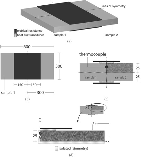
Two identical samples of PVC (polyvinyl chloride) in a symmetric assembly were used, each sample has thickness of 50 mm and lateral dimensions of $300\times 300$ mm.

The ensemble of the samples initially in thermal equilibrium at $T_0$ is then submitted to a unidirectional uniform heat flux. The heat is supplied by a 318 ohm electric resistance heater, covered with silicone rubber, with lateral dimensions of $300\times 300$ mm and thickness of 0.1 mm.

The heat flux is acquired by a transducer of lateral dimensions of $50\times 50$ mm and thickness of 0.1 mm with time constant of less than 10 ms. The transducer is based on the thermopile conception of multiple phyelectric junctions (made by electrolytic deposition) on a thin conductor sheet [16]. The temperatures are measured using type K thermocouples. The signals of heat flux and temperatures are acquired by a AGILENT model 34970A data acquisition system controlled by a personal computer.

The resistance/transducer assembly is shown in Figure 9. The thermal model of this experiment determines heating in a given area while the remaining surfaces are insulated. The condition of thermal insulation in the left face and lower surface of Figure 9(d) are obtained by the symmetrical assembly of the experiment. The remaining conditions are obtained by insulation with expanded polystyrene. Although this insulation is not perfect, its influence on the measured temperature is negligible.

The priori calibrated heat flux transducer is responsible for experimental heat flux data. The signals from these devices suffer an attenuation and a thermal delay due to their thermal resistance. The heat flux transducer and the electrical resistance are responsible for measuring and producing the heat flux that heats the sample superficially.

6. Results

The sample of polyvinyl chloride (PVC) has L=0.3030 m, W=0.0125 m and R=0.1530 m as defined in Figure 9. The experimental tests were made with the heat flux shown in Figure 10. The experimental temperatures $T_1$ and $T_2$ were obtained at the positions shown in Table 1. Figure 11(a) shows the evolution of experimental temperatures. Figure 11(b) shows $\left(T\right(t_i)-T(t_{i+1}\left)\right)$, that is, the temperature fluctuation showing the discontinuity of the data caused by the noise inherent of the experimental data.

Figure 10. Typical signal of experimental heat flux.

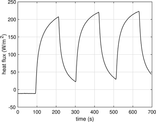
Figure 11. Experimental temperatures used to estimate the heat flux. (a) Experimental temperatures. (b) Fluctuation, $T\left(t_i\right)-T\left(t_{i+1}\right)$.

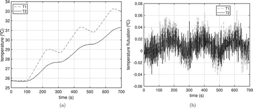
Table 1. Thermocouple locations.

location	x (m)	y (m)	z (m)
termocouple 1 ($T_1$)	0	$0.0113$	0.1
termocouple 2 ($T_2$)	0	0.0075	0.1

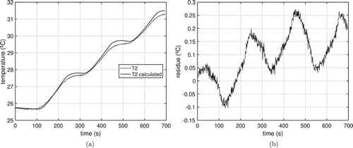
Figures 12 and 13 show the comparison between the experimental temperatures $T_1$ and $T_2$ and the temperatures calculated by Equation (17(17) $\begin{array}{rl}\theta (x,y,z,t)& =8{\theta }_0\sum _{p=1}^{\mathrm{\infty }}\sum _{m=1}^{\mathrm{\infty }}\sum _{n=1}^{\mathrm{\infty }}{\mathrm{e}}^{-\left(\frac{{\alpha }_m^2}{L^2}+\frac{{\beta }_n^2}{W^2}+\frac{{\gamma }_p^2}{R^2}\right)\alpha t}\\ & \times \left[\frac{{\alpha }_m^2+B_1^2}{{\alpha }_m^2+B_1^2+B_1}\right]\left[\frac{{\beta }_n^2+B_2^2}{{\beta }_n^2+B_2^2+B_2}\right]\left[\frac{{\gamma }_p^2+B_3^2}{{\gamma }_p^2+B_3^2+B_3}\right]\\ & \times \left[\cos \left(\frac{{\alpha }_{m}x}{L}\right)\frac{\sin {\alpha }_m}{{\alpha }_m}\right]\left[\cos \left(\frac{{\beta }_{n}y}{W}\right)\frac{\sin {\beta }_n}{{\beta }_n}\right]\\ & \times \left[\cos \left(\frac{{\gamma }_{p}z}{R}\right)\frac{\sin {\gamma }_p}{{\gamma }_p}\right]\\ & +\frac{8\alpha }{kW}\sum _{p=1}^{\mathrm{\infty }}\sum _{n=1}^{\mathrm{\infty }}\sum _{m=1}^{\mathrm{\infty }}{\mathrm{e}}^{-\left(\frac{{\alpha }_m^2}{L^2}+\frac{{\beta }_n^2}{W^2}+\frac{{\gamma }_p^2}{R^2}\right)\alpha t}\\ & \times \left[\frac{{\alpha }_m^2+B_1^2}{{\alpha }_m^2+B_1^2+B_1}\right]\left[\frac{{\beta }_n^2+B_2^2}{{\beta }_n^2+B_2^2+B_2}\right]\left[\frac{{\gamma }_p^2+B_3^2}{{\gamma }_p^2+B_3^2+B_3}\right]\\ & \times \left[\cos \left(\frac{{\alpha }_{m}x}{L}\right)\frac{\sin \left(\frac{{\alpha }_m}{2}\right)}{{\alpha }_m}\right]\left[\cos \left(\frac{{\beta }_{n}y}{W}\right)\cos {\beta }_n\right]\\ & \times \left[\cos \left(\frac{{\gamma }_{p}z}{R}\right)\frac{\sin \left(\frac{{\gamma }_p}{2}\right)}{{\gamma }_p}\right]{\int }_0^t\left[q\left(\tau \right){\mathrm{e}}^{\left(\frac{{\alpha }_m^2}{L^2}+\frac{{\beta }_n^2}{W^2}+\frac{{\gamma }_p^2}{R^2}\right)\alpha \tau }\right]\mathrm{d}\tau .\end{array}$(17) ) applying the experimental heat flux (Figure 10). The respective residues are of the order of 1.2%.

Figure 12. Experimental temperature ($T_1$) versus calculated temperature. (a) Experimental Vs calculated. (b) Residue.

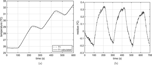
Figure 13. Experimental temperature ($T_2$) versus calculated temperature. (a) Experimental Vs calculated. (b) Residue.

For the calculation of the temperatures by Equation (17(17) $\begin{array}{rl}\theta (x,y,z,t)& =8{\theta }_0\sum _{p=1}^{\mathrm{\infty }}\sum _{m=1}^{\mathrm{\infty }}\sum _{n=1}^{\mathrm{\infty }}{\mathrm{e}}^{-\left(\frac{{\alpha }_m^2}{L^2}+\frac{{\beta }_n^2}{W^2}+\frac{{\gamma }_p^2}{R^2}\right)\alpha t}\\ & \times \left[\frac{{\alpha }_m^2+B_1^2}{{\alpha }_m^2+B_1^2+B_1}\right]\left[\frac{{\beta }_n^2+B_2^2}{{\beta }_n^2+B_2^2+B_2}\right]\left[\frac{{\gamma }_p^2+B_3^2}{{\gamma }_p^2+B_3^2+B_3}\right]\\ & \times \left[\cos \left(\frac{{\alpha }_{m}x}{L}\right)\frac{\sin {\alpha }_m}{{\alpha }_m}\right]\left[\cos \left(\frac{{\beta }_{n}y}{W}\right)\frac{\sin {\beta }_n}{{\beta }_n}\right]\\ & \times \left[\cos \left(\frac{{\gamma }_{p}z}{R}\right)\frac{\sin {\gamma }_p}{{\gamma }_p}\right]\\ & +\frac{8\alpha }{kW}\sum _{p=1}^{\mathrm{\infty }}\sum _{n=1}^{\mathrm{\infty }}\sum _{m=1}^{\mathrm{\infty }}{\mathrm{e}}^{-\left(\frac{{\alpha }_m^2}{L^2}+\frac{{\beta }_n^2}{W^2}+\frac{{\gamma }_p^2}{R^2}\right)\alpha t}\\ & \times \left[\frac{{\alpha }_m^2+B_1^2}{{\alpha }_m^2+B_1^2+B_1}\right]\left[\frac{{\beta }_n^2+B_2^2}{{\beta }_n^2+B_2^2+B_2}\right]\left[\frac{{\gamma }_p^2+B_3^2}{{\gamma }_p^2+B_3^2+B_3}\right]\\ & \times \left[\cos \left(\frac{{\alpha }_{m}x}{L}\right)\frac{\sin \left(\frac{{\alpha }_m}{2}\right)}{{\alpha }_m}\right]\left[\cos \left(\frac{{\beta }_{n}y}{W}\right)\cos {\beta }_n\right]\\ & \times \left[\cos \left(\frac{{\gamma }_{p}z}{R}\right)\frac{\sin \left(\frac{{\gamma }_p}{2}\right)}{{\gamma }_p}\right]{\int }_0^t\left[q\left(\tau \right){\mathrm{e}}^{\left(\frac{{\alpha }_m^2}{L^2}+\frac{{\beta }_n^2}{W^2}+\frac{{\gamma }_p^2}{R^2}\right)\alpha \tau }\right]\mathrm{d}\tau .\end{array}$(17) ), both the initial temperature, $T_0$, and the ambient temperature, $T_{\mathrm{\infty }}$, were $25.74{(}^{\circ }\mathrm{C})$. Thermophysical properties were k=0.152 (W/mK) and $\alpha =1.17E-07$ (m²/s) [17]. In the planes yz (at x=L) and xy (at z=R), h=10  (W/m²K) equivalent to natural convection was used. In the area adjacent to the heat flux area, h is sufficiently small to simulate thermal insulation. Time step $dt=1$ (s).

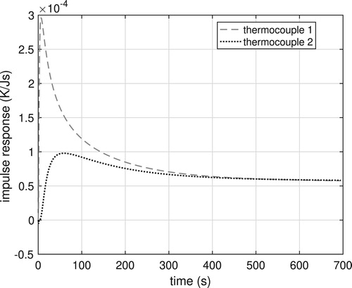
Figure 14 shows the behaviour of the impulse response calculated with Equation (20(20) $\begin{array}{rl}h(x,y,z,t)& =\frac{8\alpha }{kW}\sum _{p=1}^{\mathrm{\infty }}\sum _{n=1}^{\mathrm{\infty }}\sum _{m=1}^{\mathrm{\infty }}{\mathrm{e}}^{-\left(\frac{{\alpha }_m^2}{L^2}+\frac{{\beta }_n^2}{W^2}+\frac{{\gamma }_p^2}{R^2}\right)\alpha t}\\ & \times \left[\frac{{\alpha }_m^2+B_1^2}{{\alpha }_m^2+B_1^2+B_1}\right]\left[\frac{{\beta }_n^2+B_2^2}{{\beta }_n^2+B_2^2+B_2}\right]\left[\frac{{\gamma }_p^2+B_3^2}{{\gamma }_p^2+B_3^2+B_3}\right]\\ & \times \left[\cos \left(\frac{{\alpha }_{m}x}{L}\right)\frac{\sin \left(\frac{{\alpha }_m}{2}\right)}{{\alpha }_m}\right]\left[\cos \left(\frac{{\beta }_{n}y}{W}\right)\cos {\beta }_n\right]\\ & \times \left[\cos \left(\frac{{\gamma }_{p}z}{R}\right)\frac{\sin \left(\frac{{\gamma }_p}{2}\right)}{{\gamma }_p}\right]\end{array}$(20) ) for the positions of (Table 1). It shows the damped behaviour of the impulse response function at the position of $T_2$, which is further away from the heat source, and therefore, with less sensitivity. As the impulse response acts as a filter, this damping is one of the factors which makes it difficult to estimate the heat flux using the information of this position.

Figure 14. Impulse response.

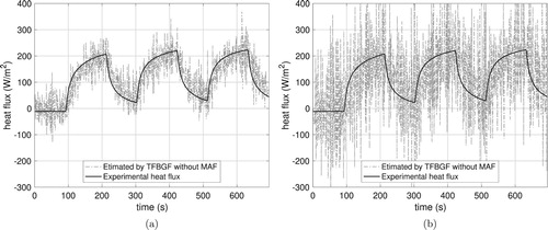
Applying the TFBGF technique, the heat flux is estimated by means of the impulse response and the experimental temperature. Figure 15 shows attempts to estimate heat flux without the use of the moving average filter. The noise present in the experimental temperature is amplified in the estimate of the heat flux. The ill-conditioning nature of the problem is clear.

Figure 15. Experimental heat flux and estimated heat flux (by TFBGF) without moving average filter (MAF). (a) From $T_1$. (b) From $T_2$.

As a strategy to transform the poorly-conditioned problem into an approximate well-conditioned problem the moving average filter was applied. The moving average can be applied to the temperature vector (in the input) or the heat flux estimation vector, since it is a linear problem.

To analyse the choice of the size N of the moving average, the mean square error (ERMS) was calculated. Table 2 shows the ERMS for the estimation of the heat flux using the experimental temperatures $T_1$ and $T_2$.

Table 2. ERMS error for different sizes $\left(N\right)$ of moving average.

N	filt. $T_1$	filt. $T_2$	filt. $q\left(T_1\right)$	filt. $q\left(T_2\right)$
1	53.1102	148.9666	53.1102	148.9666
2	30.9874	84.1824	30.9948	84.1972
3	25.0706	60.0461	25.0950	60.0745
4	20.5264	48.3253	20.5420	48.3557
5	18.8339	42.2404	18.8573	42.2811
6	16.7481	37.6493	16.7700	37.6708
7	16.0024	34.5721	16.0421	34.6078
8	15.2256	31.8608	15.2696	31.8774
9	15.0146	30.4425	15.0669	30.4546
10	15.2119	28.6195	15.2694	28.6332
11	15.4659	27.6272	15.5184	27.6388
12	16.6897	26.3038	16.7389	26.3031
13	17.1090	25.5668	17.1606	25.5634
14	18.8794	24.8884	18.9233	24.8770
15	19.4848	24.6888	19.5326	24.6751
16	21.5415	24.3562	21.5894	24.3307
17	22.2418	24.2441	22.2888	24.2206
18	24.4785	24.4282	24.5223	24.3857
19	25.2072	24.4782	25.2527	24.4311
20	27.4969	25.1483	27.5331	25.0939

Columns 1 and 2 (Table 2) show that the lowest quadratic error value between experimental and estimated heat flux was obtained with moving average filter of N=9 for $T_1$ and N=17 for $T_2$.

Table 2 shows the different ERMS values for $N=1,\dots ,20$. The problem of finding an optimal value of N can be reduced to a search within an initial interval $N_1<N<N_2$. In Figure 4 it is observed that for N very large the ERMS will be increasing.

The option to apply the moving average as a filter is due to the ease of implementation of the algorithm, its low computational cost and its efficiency.

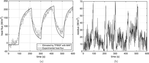
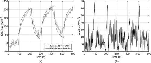
Figures 16 and 17 show the experimental heat flux and the estimated heat flux and the absolute residues, obtained from positions/temperatures $T_1$ and $T_2$ respectively.

Figure 16. Estimated heat flux (using $T_1$) with moving average filter $(N=9)$ in temperature vector. (a) From $T_1$. (b) Absolute residue.

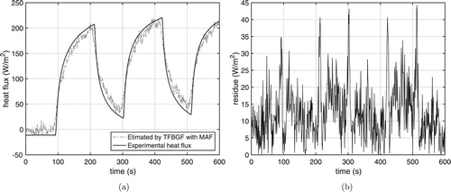
Figure 17. Estimated heat flux (using $T_2$) with moving average filter $(N=17)$ in temperature vector. (a) From $T_2$. (b) Absolute residue.

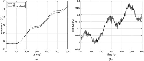
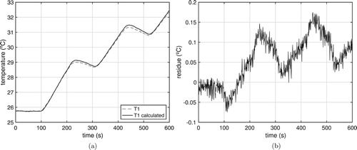
The estimated heat flux from position $T_1$ (Figure 16) whose ERMS is 15.01, is applied to the direct problem given by Equation (17(17) $\begin{array}{rl}\theta (x,y,z,t)& =8{\theta }_0\sum _{p=1}^{\mathrm{\infty }}\sum _{m=1}^{\mathrm{\infty }}\sum _{n=1}^{\mathrm{\infty }}{\mathrm{e}}^{-\left(\frac{{\alpha }_m^2}{L^2}+\frac{{\beta }_n^2}{W^2}+\frac{{\gamma }_p^2}{R^2}\right)\alpha t}\\ & \times \left[\frac{{\alpha }_m^2+B_1^2}{{\alpha }_m^2+B_1^2+B_1}\right]\left[\frac{{\beta }_n^2+B_2^2}{{\beta }_n^2+B_2^2+B_2}\right]\left[\frac{{\gamma }_p^2+B_3^2}{{\gamma }_p^2+B_3^2+B_3}\right]\\ & \times \left[\cos \left(\frac{{\alpha }_{m}x}{L}\right)\frac{\sin {\alpha }_m}{{\alpha }_m}\right]\left[\cos \left(\frac{{\beta }_{n}y}{W}\right)\frac{\sin {\beta }_n}{{\beta }_n}\right]\\ & \times \left[\cos \left(\frac{{\gamma }_{p}z}{R}\right)\frac{\sin {\gamma }_p}{{\gamma }_p}\right]\\ & +\frac{8\alpha }{kW}\sum _{p=1}^{\mathrm{\infty }}\sum _{n=1}^{\mathrm{\infty }}\sum _{m=1}^{\mathrm{\infty }}{\mathrm{e}}^{-\left(\frac{{\alpha }_m^2}{L^2}+\frac{{\beta }_n^2}{W^2}+\frac{{\gamma }_p^2}{R^2}\right)\alpha t}\\ & \times \left[\frac{{\alpha }_m^2+B_1^2}{{\alpha }_m^2+B_1^2+B_1}\right]\left[\frac{{\beta }_n^2+B_2^2}{{\beta }_n^2+B_2^2+B_2}\right]\left[\frac{{\gamma }_p^2+B_3^2}{{\gamma }_p^2+B_3^2+B_3}\right]\\ & \times \left[\cos \left(\frac{{\alpha }_{m}x}{L}\right)\frac{\sin \left(\frac{{\alpha }_m}{2}\right)}{{\alpha }_m}\right]\left[\cos \left(\frac{{\beta }_{n}y}{W}\right)\cos {\beta }_n\right]\\ & \times \left[\cos \left(\frac{{\gamma }_{p}z}{R}\right)\frac{\sin \left(\frac{{\gamma }_p}{2}\right)}{{\gamma }_p}\right]{\int }_0^t\left[q\left(\tau \right){\mathrm{e}}^{\left(\frac{{\alpha }_m^2}{L^2}+\frac{{\beta }_n^2}{W^2}+\frac{{\gamma }_p^2}{R^2}\right)\alpha \tau }\right]\mathrm{d}\tau .\end{array}$(17) ). Figures 18 and 19 show the experimental and estimated temperatures obtained with the estimated heat flux from position $T_1$ and the moving average filter (N=9).

Figure 18. Experimental temperature ($T_1$) versus calculated temperature using estimated heat flux. (a) Experimental Vs calculated. (b) Residue.

Figures 16 and 17 show that the heat flux estimation with the moving average filter was obtained successfully. In both cases the residues between calculated and experimental temperatures were within the limits of the experimental random errors of temperature, i.e. less than ${0.3}^{\circ }$C.

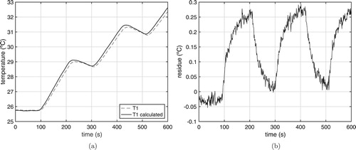
Figure 19. Experimental temperature ($T_2$) versus calculated temperature using estimated heat flux. (a) Experimental Vs calculated. (b) Residue.

As shown in Figure 7, the moving average filter can be applied after the convolution (Equation (6(6) $q\left(t\right)=T(\mathbf{x},t)\ast {\mathcal{L}}^{-1}\left\{1/H\right(\mathbf{x},s\left)\right\}.$(6) )), i.e. without the experimental temperatures being pre-filtered. The moving average filter will be applied to the heat flux shown in Figure 15. Columns three and four of Table 2 show the ERMS for each moving average size N applied directly to the heat flux vector. Table 2 and Figures 20 and 21 show that there is no significant difference between the application a priori (temperature) or posteriori (heat flux) of the moving average filter.

Figure 20. Estimated heat flux applying moving average filter $(N=9)$ in heat flux vector. (a) From $T_1$. (b) Absolute residue.

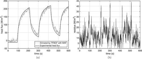
Figure 21. Estimated heat flux applying moving average filter $(N=17)$ in heat flux vector. (a) From $T_2$. (b) Absolute residue.

Given the linear treatment of the solution of the direct and inverse problem presented in Section 2, it can also be observed that in the convolution $T(x,t)=h(x,t)\ast q\left(t\right)$, if $q\left(t\right)$ is replaced by the estimated heat flux $q_{\mathrm{e}\mathrm{s}\mathrm{t}}=q\left(t\right)\pm \delta \left(t\right)$, where $\delta \left(t\right)$ is the error amplified by noise in the temperature, and in the domain of the variable s is expressed as $\delta \left(s\right)=\epsilon \left(s\right)/H(\mathbf{x},s)$), therefore (22) $\begin{array}{rl}T(\mathbf{x},t)& =h(\mathbf{x},t)\ast [q\left(t\right)\pm \delta \left(t\right)]\Rightarrow \\ T(\mathbf{x},s)& =H(\mathbf{x},s)q\left(s\right)\pm H(\mathbf{x},s)\delta \left(s\right)\Rightarrow \\ T(\mathbf{x},t)& =h(\mathbf{x},t)\ast q\left(t\right)\pm \epsilon \left(t\right)\end{array}$(22) Which signifies that the amplified error in the estimation of the heat flux is annihilated in the direct problem solution. The estimate for the heat flux shown in Figure 15 when applied to the solution of the direct problem by Green's functions (Equation (15(15) $\begin{array}{rl}& \theta (x,y,z,t)\\ & ={\int }_{x^{\prime }=0}^L{\int }_{y^{\prime }=0}^W{\int }_{z^{\prime }=0}^{R}G(x,y,z,t|x^{\prime },y^{\prime },z^{\prime },0){\theta }_0\mathrm{d}{x}^{\prime }\mathrm{d}{y}^{\prime }\mathrm{d}{z}^{\prime }\\ & +\frac{\alpha }{k}{\int }_{\tau =0}^t{\int }_{x^{\prime }=0}^{L/2}{\int }_{z^{\prime }=0}^{R}q\left(\tau \right)G(x,y,z,t|x^{\prime },W,z^{\prime },\tau )\mathrm{d}{x}^{\prime }\mathrm{d}{z}^{\prime }\mathrm{d}\tau .\end{array}$(15) )) describes the temperature successfully as shown in Figure 22, with residue less than ${0.2}^{\circ }$C.

Figure 22. Experimental temperature ($T_1$) versus calculated temperature. (a) Experimental Vs calculated. (b) Residue.

7. Conclusion

This work evaluates the application of the moving average filter in conjunction with the TFBFG method, whose objective is to convert poorly conditioned problems into approximate well-conditioned problems. In the TFBFG method the solution of the inverse problem identifies the analytical transfer function by means of Green's functions. It is a simple approach without iterative processes, and therefore extremely fast. As the technique uses the principle of linear superposition and deconvolution, any noise due to errors in temperature measurement is directly transported and amplified for the estimated heat flux components. In this case, some regularization method may be necessary to add stability to the inverse solution. The regularization procedure proposed here is the moving average filters.

As the technique is based on the principle of linear superposition, the moving average filter can be applied both a priori, that is, to the temperature vector, and a posteriori, to the heat flux vector.

In this work, an experimental procedure was designed to demonstrate the ability and technical robustness of TFBGF method with the regularization considering temperature data in regions of low sensitivity and high experimental uncertainty.

Acknowledgements

The authors thank the researchers Luis Henrique Ignacio, Alisson Figueiredo and Fernando Costa Malheiros for the great help in the experimental execution, and to the research funding agencies CNPq, CAPES and FAPEMIG.

Disclosure statement

No potential conflict of interest was reported by the authors.

Additional information

Funding

This work was supported by Coordenação de Aperfeiçoamento de Pessoal de Nível Superior [grant number PNPD20131329].

Notes

1 The element of a set of numbers that when combined with another number in a particular operation leaves that number unchanged.

References

- Beck J, Blackwell B, Clair C. Inverse heat conduction: Ill-posed problems. New York (NY): Wiley; 1985.
- Woodbury KA, Beck JV, Najafi H. Filter solution of inverse heat conduction problem using measured temperature history as remote boundary condition. Int J Heat Mass Transf. 2014;72:139–147. doi: 10.1016/j.ijheatmasstransfer.2013.12.073
- Samadi F, Woodbury K, Beck J. Evaluation of generalized polynomial function specification methods. Int J Heat Mass Transf. 2018;122:1116–1127. Available from: http://www.sciencedirect.com/science/article/pii/S001793101735086X doi: 10.1016/j.ijheatmasstransfer.2018.02.018
- Keanini RG, Ling X, Cherukuri HP. A modified sequential function specification finite element-based method for parabolic inverse heat conduction problems. Comput Mech. 2005;36(2):117–128. doi: 10.1007/s00466-004-0644-3
- Woodbury KA, Beck JV. Estimation metrics and optimal regularization in a tikhonov digital filter for the inverse heat conduction problem. Int J Heat Mass Transf. 2013;62:31–39. doi: 10.1016/j.ijheatmasstransfer.2013.02.052
- Cabeza JMG, García JAM, Rodríguez AC. A sequential algorithm of inverse heat conduction problems using singular value decomposition. Int J Therm Sci. 2005;44(3):235–244. Available from: http://www.sciencedirect.com/science/article/pii/S1290072904001838 doi: 10.1016/j.ijthermalsci.2004.06.009
- Rajabpour A, Kowsary F, Esfahanian V. Reduction of the computational time and noise filtration in the ihcp by using the proper orthogonal decomposition (pod) method. Int Commun Heat Mass Transf. 2008;35(8):1024–1031. Available from: http://www.sciencedirect.com/science/article/pii/S0735193308001024 doi: 10.1016/j.icheatmasstransfer.2008.05.004
- Shenefelt J, Luck R, Taylor R, et al. Solution to inverse heat conduction problems employing singular value decomposition and model-reduction. Int J Heat Mass Transf. 2002;45(1):67–74. Available from: http://www.sciencedirect.com/science/article/pii/S0017931001001296 doi: 10.1016/S0017-9310(01)00129-6
- Alifanov OM. Solution of an inverse problem of heat conduction by iteration methods. J Eng Phys Thermophys. 1974;26(4):471–476. doi: 10.1007/BF00827525
- Özişik MN, Orlande HRB. Inverse heat transfer. New York (NY): Taylor & Francis; 2000.
- Ahmadi-Noubari H, Pourshaghaghy A, Kowsary F, et al. Wavelet application for reduction of measurement noise effects in inverse boundary heat conduction problems. Int J Numer Methods Heat Fluid Flow. 2008;18(2):217–236. doi: 10.1108/09615530810846356
- Farahani SD, Kowsary F. Comparison of the molliffication method, wavelet transform and moving average filter for reduction of measurement noise effects in inverse heat conduction problems. Transaction B. 2010;17(4):301–314.
- Fernandes AP Analytical transfer function applied to solve IHCP [dissertation]. Federal University of Uberlândia; 2013. (in Portuguese).
- Cole KD, Beck JV, Haji-Sheikh A, et al. Heat conduction using Green's functions. Boca Raton (FL): Taylor & Francis Group; 2010. (Series in computational and physical processes in mechanics and thermal sciences).
- Smith SW. The scientist and engineer's guide to digital signal processing. San Diego: California Technical Publishing; 1998.
- Guimarães G, Philippi PC, Thery P. Use of parameters estimation method in the frequency domain for the simultaneous estimation of thermal diffusivity and conductivity. Rev Sci Instrum. 1995;66(3):2582–2588. doi: 10.1063/1.1145592
- Borges VL, Lima e Silva SMM, Guimarães G. A dynamic thermal identification method applied to conductor and nonconductor materials. Inverse Probl Sci Eng. 2006;14(5):511–527. doi: 10.1080/17415970600573700