Prediction of nonlinear viscoelastic behaviour of simulative soil for deep-sea sediment using a thermodynamically compatible model

ABSTRACT

This work focuses on the development of a suitable theoretical model for defining the nonlinear viscoelastic behaviour of deep-seabed sediments. To that end, shear rheological tests are performed on simulative soil samples at different shear rates. These samples are prepared by mixing bentonite with water based on the in situ vane shear strength of deep-sea sediments. A nonlinear viscoelastic fluid model based on a thermodynamic standpoint is derived by considering two scalar functions. The two scalar functions, namely, the stored energy and the rate of dissipation are found using the nonlinear response of the samples collected from experiments. This novel approach identifies the model parameters having physical significance and has considerable advantages over previous models which are predominantly empirical. This is carried out as an inverse problem in which the parameters are estimated by minimizing the deviation between the predicted and measured torque response of the sample when subjected to shear rheometry with the shear rate as the input. The efficacy of the model has been investigated and reasonable agreement with the peak as well as steady-state values of torque is observed.

KEYWORDS:

• Deep-sea sediments
• shear rheology
• nonlinear viscoelasticity
• theoretical model
• inverse problem
• parameter identification

2010 MATHEMATICS SUBJECT CLASSIFICATION:

• 74D10

1. Introduction

In recent times, mineral resources which are abundant in the deep-seabed have received significant global attention [1]. Scientists and engineers have been keenly involved in developing an undersea mining machine which can collect the deep-sea minerals (known as Poly-metallic nodules) from the seabed. Recent technologies use remotely operated undercarriage tracked vehicles (crawlers) to collect minerals from prospective mine sites [2,3].

The movement of mining vehicle on soft cohesive soil is one of the major challenges in deep-sea mining as its traction is decided by shear strength of the deep-sea sediments. Deep-sea sediments have higher water content and lower shear strength than ordinary land soils [4]. Therefore, the mining vehicle can slip easily and becomes immobile as it moves past the seabed surface. Owing to the difficulty in obtaining the deep-sea sediments for large scale of experimental studies, bentonite-water mixtures have been used as the best substitutive for deep-sea sediments by many researchers [5,6]. The deep-sea sediment substitute is prepared by mixing the bentonite with water at a proper ratio till the bentonite paste material has the same vane shear strength as the deep-sea sediment in situ. The widely used bentonite clay resemble the original deep-sea sediments (physical and mechanical characteristics in most of the aspects) [7].

For the optimization of traction of the mining vehicle, it is desirable to determine the estimation of trafficability of the seafloor surface. Hence, based on various test and experimental analysis (shear ring, vane test, track segment shear tests) in the bentonite-water mixture (deep-sea sediment simulacrum), different empirical relations for sea bed sediments have been developed [8–10]. However, these relations vary significantly with the types of testing. Moreover, the time-dependent effect of deep-sea sediment is not considered in the above studies. Some attempts have been made to explore the time-dependent effect of deep-sea sediments based on the experiments conducted in the bentonite-water mixture. Ma et al. [7] studied shear creep characteristics on the simulative soil of shear strength ranging from 1 to 5 kPa by shear creep test and shear creep parameters are found out by adopting the Burgers rheological model [11]. Recently, Xu et al. [12] derived compression-shear coupling rheological model based on the compression-shear creep experiments and the compression-shear coupling rheological parameters are identified.

While considering the bentonite suspensions in a variety of industrial applications mainly from the drilling fluid industry point of view. Research has been done focusing on bentonite suspensions thixotropic behaviour, wherein the bentonite suspension contains at least $90\mathrm{\%}$ of water [13]. The bentonite suspensions are quite complex by their thixotropy, which involves the monotonically decreasing shear stress with time when the fluid is subjected to a constant shear rate, and to recover these properties progressively when the shear rate is relieved [14]. By considering this behaviour, measurement on rheological properties of bentonite suspensions has been reported by many researchers [15,16].

The phenomenon for the thixotropic behaviour of bentonite suspensions with different mass concentrations was studied by Bekkour et al. [17] using different experimental procedures. It was found that the bentonite dispersions exhibit a time-dependent non-Newtonian behaviour and major factors affecting the rheological properties in the dispersion were the value of shear rate and duration. Bekkour and Kherfellah [18] conducted creep and oscillatory shear experiments in the linear viscoelastic domain on bentonite-water suspensions at different solid fractions. It was found that bentonite dispersions exhibit viscoelastic behaviour for concentrations higher than 6% by weight and the generalized Kelvin–Voigt mechanical model is used to describe the behaviour.

From the above literature survey, it is clear that an understanding of the rheological behaviour of the bentonite-water mixture is of vital importance since such materials are being used as a substitute for deep-sea sediments. Though deep-sea sediments have been used extensively from prehistoric times, development of accurate theoretical models is an ongoing important area of research. However, the development of theoretical models is still based on the linearized theory of viscoelasticity. Therefore, the concentrated bentonite suspension offers a unique opportunity in developing models using nonlinear constitutive relations. This work focuses on the nonlinear viscoelastic model that has been developed from a thermodynamic framework [19], that generally covers the physical behaviour for a range of material media. This novel extension to deep-sea sediments seeks improved accuracy and consistency in the formulation of nonlinear constitutive relations and in the identification of model parameters based on torsion experiments conducted in the simulative soil (bentonite-water mixture) samples. The key feature of the thermodynamic framework used in this study is that the model response is entirely determined by the knowledge of two scalar potentials namely, the stored energy function and the rate of dissipation function.

2. Experiment

2.1. Materials and sample preparation

Commercially available sodium bentonite was used to prepare the simulative soil samples. As the sample under consideration is a substitute for deep-sea sediments, more attention was given to assure that the geotechnical properties are matching with field data available for deep-sea sediments. Deep-sea sediments have higher water content and exhibit entirely different shear properties than land soils [4]. Soft soils having a very low shear strength ranging from 1 to 3 kPa are encountered on the top layer of the deep-seabed and it affects the stability of the structures placed thereon [20,21]. Therefore, the sample preparations have been made based on these considerations. The appropriate amount of water was added to bentonite so as to match its shear strength with deep-sea clay. The water content of the samples prepared decides the shear strength in the desired range.

The sample preparation procedure has a great impact on the final state of the suspensions and thus on the rheological behaviour. Hence, an identical procedure was followed each time. Initially, bentonite powder sieved through 75-µm sieve to remove lumps and impurities. It was then dried in an oven at ${102}^{\circ }\mathrm{C}$ to remove the traces of natural moisture content. It is well established that the pH value and the ion content of the water are important parameters related to the inner structure of the suspension [22]. Hence, bentonite powder was dispersed in the required amount of deionized water with no chemical additives. Since the amount of sample required for the experiment is very low, homogenization was achieved by continuous mechanical agitation through thorough hand mixing for an hour by squeezing the sample in airtight ziplock bag/cover. The sample obtained was used for experiments. Table 1 shows the constitution of various simulative soils (bentonite-water mixture) samples ranging from 1 to 3 kPa. It can be seen that the shear strength of the sample increases as the percentage of water content decreases from 85% to 70%.

Table 1. Shear strength variation with water content in simulative soil samples.

		Water content
Sample no.	Bentonite weight (g)	Weight (g)	Percentage of water	Ratio of mass of water to mass of bentonite	Approximate shear strength (kPa)
1	6	34	85	5.66	$<1$
2	8	32	80	4	1
3	10	30	75	3	3
4	12	28	70	2.33	$>3$

2.2. Experimental set up and procedures

Samples with shear strength ranging from 1 to 3 kPa were considered for experimental studies since it could better represent the soil on the top of the sea-bed which has low shear strength, as discussed in Section 2.1. The evolution of samples over time was studied with the application of shear rheometry. Rheological tests allow more fundamental investigation compared to other tests. Furthermore, it provides a precise description of flow properties and serves as input for numerical simulations.

Anton-Paar MCR 301 Rheometer was used for this study (shown in Figure 1). The loading and unloading of samples in the parallel plate geometry has been found more suitable than cone-and-plate or concentric cylinder geometries for shearing the type of concentrated suspensions used in this work [23]. Thus, the parallel plate rheometry was used.

Figure 1. Photograph of Anton-Paar MCR 301 Rheometer with bentonite-water mixture sample.

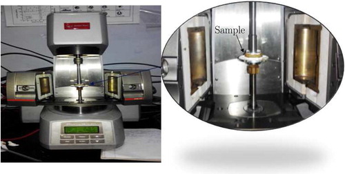
Here, the sample was contained between an upper rotating flat stainless steel disc and a lower stationary disc sharing a common axis. The samples are carefully loaded on the stationary plate of the rheometer with a spatula and then the desired gap of 2 mm was maintained. While maintaining the desired gap, the squeezing of the sample occurs and leads to an increase in normal stress of the sample. Hence, before starting the test, the normal stress created by the squeezing motion was allowed to relax to its steady-state value. The extra material squeezed out of parallel plate was trimmed off. The complete geometry was covered by a vapour hood for retaining moisture in the sample during the test. All the tests were conducted at a constant temperature equal to ${25}^{\circ }\mathrm{C}$. The flow occurs between the rheometer stationary bottom plate and the rotating top plate and is schematically shown in Figure 2(a).

Figure 2. Parallel plate geometry: (a) torsional flow of the sample and (b) enlarged view of parallel plate disc with sandpaper.

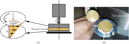
The serious slip effects (wall effects) can be minimized by increasing the roughness of rotating discs. Therefore, this geometry was modified by bonding the waterproof sandpaper (with a grit size of 200  µm) using the double-sided adhesive tape as shown in Figure 2(b). When the slip effects are minimal, small variations in the gap between the plates does not affect the results. The modified parallel plate geometry was again validated by assuring the repeatability of results.

The time-dependent response of the sample was investigated by torsional shear, strain rate-controlled mode. This involves holding the sample at a constant shear rate and then the torsional force produced on the top plate was measured as a function of time. The shear rate was computed as $\gamma =\omega R/h$ in a parallel plate geometry. Therefore, the angular velocity ω (rad ${\mathrm{s}}^{-1}$) calculated at the edge of the top rotating plate was maintained at a steady value in the shear rate-controlled mode. At each loading condition, the samples were tested at least twice to ensure the accuracy and fairly repeatable results were observed. The shear rates of 0.1, 1 and $10{\mathrm{s}}^{-1}$ were considered in our study. The diameter of the plate is $R=12.5\mathrm{mm}$ and a constant gap of $h=2\mathrm{mm}$ was maintained during the measurements. Obviously, for each shear rates, a fresh sample was used.

2.3. Experimental results

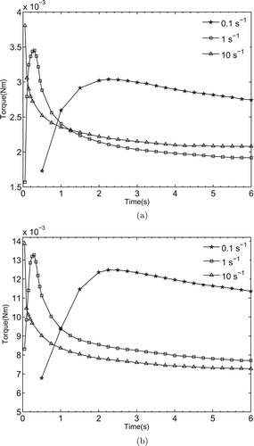
The evolution of torque with time in simulative soil (bentonite-water mixture) samples at different values of shear rate is illustrated in Figure 3. For brevity, only the results for the 20 and 25 wt.% bentonite-water mixture (samples 2 and 3) is shown, the other concentrations (samples 1 and 4), as in Table 1, follow the same trend. The results of the experiments clearly show that the simulative soil samples used in this study exhibit non-linear response. When the samples are subjected to different shear rates, the torque produced by this transient deformation displays an initial overshoot before reaching a steady-state value. However, the initial overshoot behaviour of torque is not captured at a very high rate of $10{\mathrm{s}}^{-1}$ due to the very fast destructuration of the sample. Since torque is proportional to shear stress, the initial increase in torque with time indicates the elastic strain of the material. At a certain angle, the sample starts flowing above a critical torque. The time-dependent changes in torque can be described with periods. The first period corresponds to the elastic strain of the material. The second corresponds to flow and break down of the structure. The order of magnitude of the time scale in the first period is shorter than that in the second which shows viscous behaviour is more predominant in this sample. In addition, the experimental data shows that for the same shear rate, the value of torque maxima increases with increasing bentonite concentration. Thus the peak and steady-state values of torques are strongly affected by the imposed shear rate value and the water content. Moreover, it is noted that zero normal stress is recorded shortly after the start of most experiments. Further studies are needed to clarify the problem.

Figure 3. Evolution of torque with time in simulative soil samples at various shear rates: (a) sample with a shear strength of 1 kPa and (b) sample with a shear strength of 3 kPa.

3. Theoretical model formulation

As mentioned in Section 1, some attempts have been made using linear viscoelastic models to describe the response of bentonite-water mixture. The linear viscoelastic model is remarkably a successful model that relied on the fact that the applied stresses are relatively small so that only small strains are involved. However, from the above experimental studies, it can be observed that the variation of torque with time at various shear rates is clearly nonlinear. Hence it is difficult to interpret these characteristics using traditional linearized viscoelastic models. In view of this, it is required to develop a nonlinear constitutive relation which is capable of predicting a wide range of deformations with a reasonable accuracy.

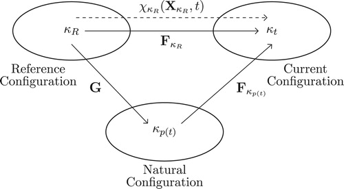
The thermodynamic framework developed in [19] is used in modelling the nonlinear response of simulative soils (bentonite-water mixtures) at different shear rates. Málek and Rajagopal [24] generalized this framework to derive a unique constitutive relation for the Cauchy stress tensor by using the same concept. In this framework, the constitutive relation for the stress is determined by making judicious assumptions regarding the manner in which the body stores and dissipates energy. This can be achieved through two scalar functions namely, the stored energy function and the rate of dissipation function which are associated with the body. According to the thermodynamic framework, the body occupies a deformed current configuration owing to the action of external stimuli. A configuration referred to as ‘natural configuration’ of the body is attained by removing the external stimuli. Thus the viscoelastic response is determined by stored energy function (Helmholtz potential) related to the elastic response from the natural configuration and a rate of dissipation function which describes the rate of dissipation due to the viscous effects. As the underlying natural configuration evolves, a change in it is determined using a thermodynamic criterion, namely, maximizing the rate of dissipation (in general, the rate of entropy production). This evolution of the natural configuration leads to rate type constitutive models. Thus, the framework guarantees that the models that are derived automatically satisfy the second law of thermodynamics. Many popular rate type models including Maxwell model and Oldroyd-B model has been derived using the same procedure [25]. In particular, some viscoelastic fluid models have been developed using this framework which can predict shear stresses and torque during torsion experiments [26,27].

This methodology for developing nonlinear constitutive relations is somehow preferable over previous methods. Instead of directly proposing a constitutive relation for the Cauchy stress tensor, which has six independent components, here we are choosing constitutive relations for two scalar quantities.

3.1. Kinematics

Let ${\kappa }_R$ denote the reference configuration and ${\kappa }_t$ denote the current configuration of a viscoelastic fluid of interest (see Figure 4). The motion function ${\chi }_{{\kappa }_R}$ is a one-to-one mapping that assigns each position ${\mathbf{X}}_{{\kappa }_R}\in {\kappa }_R$ to a corresponding position $\mathbf{x}\in {\kappa }_t$ at each time t>0, (1) $\mathbf{x}:={\chi }_{{\kappa }_R}({\mathbf{X}}_{{\kappa }_R},t).$(1) For the derivatives to exist, the motion function is assumed to be sufficiently smooth. The deformation gradient is defined through (2) ${\mathbf{F}}_{{\kappa }_R}:=\frac{d{\chi }_{{\kappa }_R}}{d{\mathbf{X}}_{{\kappa }_R}}.$(2) The left and right Green–Cauchy stretch tensors are given by (3) ${\mathbf{B}}_{{\kappa }_R}:={\mathbf{F}}_{{\kappa }_R}{\mathbf{F}}_{{\kappa }_R}^{\mathrm{T}}\mathrm{and}{\mathbf{C}}_{{\kappa }_R}:={\mathbf{F}}_{{\kappa }_R}^{\mathrm{T}}{\mathbf{F}}_{{\kappa }_R}.$(3) The principal invariants of ${\mathbf{B}}_{{\kappa }_R}$ are denoted by $I_{{\kappa }_R}$, $I{I}_{{\kappa }_R}$ and $II{I}_{{\kappa }_R}$: (4) $I_{{\kappa }_R}:=\mathrm{tr}({\mathbf{B}}_{{\kappa }_R}),I{I}_{{\kappa }_R}:=\frac{1}{2}\{{[\mathrm{tr}({\mathbf{B}}_{{\kappa }_R})]}^2-\mathrm{tr}({\mathbf{B}}_{{\kappa }_R}^2)\},II{I}_{{\kappa }_R}:=\det ({\mathbf{B}}_{{\kappa }_R}).$(4) Let ${\kappa }_{p(t)}$ denote the stress-free configuration that is reached by the instantaneous unloading of the body, which is at the configuration ${\kappa }_t$ as depicted in Figure 4.

Figure 4. Schematic diagram illustrating the notion of current natural configuration of the material.

The deformation gradient can be multiplicatively decomposed as (5) ${\mathbf{F}}_{{\kappa }_R}={\mathbf{F}}_{{\kappa }_{p(t)}}\mathbf{G},$(5) where ${\mathbf{F}}_{{\kappa }_{p(t)}}$ is the gradient of the mapping from ${\kappa }_{p(t)}$ to ${\kappa }_t$ and G is the gradient of the mapping from ${\kappa }_R$ to ${\kappa }_{p(t)}$.

The velocity gradient $\mathbf{L}$ and ${\mathbf{L}}_{{\kappa }_{p(t)}}$: (6) $\mathbf{L}:={\dot{\mathbf{F}}}_{{\kappa }_R}{\mathbf{F}}_{{\kappa }_R}^{-1},{\mathbf{L}}_{{\kappa }_{p(t)}}:=\dot{\mathbf{G}}{\mathbf{G}}^{-1}.$(6) The symmetric part of the velocity gradient tensor are (7) $\mathbf{D}:=\frac{\mathbf{L}+{\mathbf{L}}^{\mathrm{T}}}{2},{\mathbf{D}}_{{\kappa }_{p(t)}}:=\frac{{\mathbf{L}}_{{\kappa }_{p(t)}}+{\mathbf{L}}_{{\kappa }_{p(t)}}^{\mathrm{T}}}{2}.$(7) The left and right Green–Cauchy stretch tensors associated with the tensor ${\mathbf{F}}_{{\kappa }_{p(t)}}$ are (8) ${\mathbf{B}}_{{\kappa }_{p(t)}}:={\mathbf{F}}_{{\kappa }_{p(t)}}{\mathbf{F}}_{{\kappa }_{p(t)}}^{\mathrm{T}}\mathrm{and}{\mathbf{C}}_{{\kappa }_{p(t)}}:={\mathbf{F}}_{{\kappa }_{p(t)}}^{\mathrm{T}}{\mathbf{F}}_{{\kappa }_{p(t)}}.$(8) Accordingly, the principal invariants of the tensor ${\mathbf{B}}_{{\kappa }_p(t)}$ are defined as (9) $I_{{\kappa }_{p(t)}}:=\mathrm{tr}({\mathbf{B}}_{{\kappa }_{p(t)}}),I{I}_{{\kappa }_{p(t)}}:=\frac{1}{2}\{{[\mathrm{tr}({\mathbf{B}}_{{\kappa }_{p(t)}})]}^2-\mathrm{tr}({\mathbf{B}}_{{\kappa }_{p(t)}}^2)\},II{I}_{{\kappa }_{p(t)}}:=\det ({\mathbf{B}}_{{\kappa }_{p(t)}}).$(9) The upper convected Oldroyd derivative of ${\mathbf{B}}_{{\kappa }_p(t)}$ is defined through (10) ${\stackrel{\mathrm{\nabla }}{\mathbf{B}}}_{{\kappa }_{p(t)}}={\dot{\mathbf{B}}}_{{\kappa }_{p(t)}}-\mathbf{L}{\mathbf{B}}_{{\kappa }_{p(t)}}-{\mathbf{B}}_{{\kappa }_{p(t)}}{\mathbf{L}}^{\mathrm{T}}=-2{\mathbf{F}}_{{\kappa }_{p(t)}}{\mathbf{D}}_{{\kappa }_{p(t)}}{\mathbf{F}}_{{\kappa }_{p(t)}}^{\mathrm{T}}.$(10) We shall assume that the material is incompressible, which implies that (11) $\det {\mathbf{F}}_{{\kappa }_R}=1.$(11) It also follows from the incompressibilty of the elastic response that (12) $\det {\mathbf{F}}_{{\kappa }_{p(t)}}=1\Rightarrow \det {\mathbf{B}}_{{\kappa }_{p(t)}}=1.$(12) Differentiation of (11(11) $\det {\mathbf{F}}_{{\kappa }_R}=1.$(11) ) and (12(12) $\det {\mathbf{F}}_{{\kappa }_{p(t)}}=1\Rightarrow \det {\mathbf{B}}_{{\kappa }_{p(t)}}=1.$(12) ) with respect to time leads to (13) $\mathrm{tr}\mathbf{D}=\mathrm{tr}{\mathbf{D}}_{{\kappa }_{p(t)}}=0.$(13)

3.2. Balance laws

For the description of the flow of a nonlinear viscoelastic fluid, the spatial description at the current configuration ${\kappa }_t$ is used. In this section, we summarize the balance of laws in the local form (assuming continuity of integrand for arbitrary sub-parts of a body).

The balance of mass for a material with a single constituent is given through (14) $\frac{\mathrm{\partial }\rho }{\mathrm{\partial }t}+\mathrm{div}(\rho \mathbf{v})=0,$(14) where ρ is the local density of a material and v is the velocity. If a material is incompressible, Equation (14(14) $\frac{\mathrm{\partial }\rho }{\mathrm{\partial }t}+\mathrm{div}(\rho \mathbf{v})=0,$(14) ) reduces to (15) $\mathrm{div}(\mathbf{v})=0.$(15) The balance of linear momentum is (16) $\mathrm{div}({\mathbf{T}}^{\mathrm{T}})+\rho \mathbf{b}=\rho (\frac{\mathrm{\partial }\mathbf{v}}{\mathrm{\partial }t}+[\mathrm{grad}(\mathbf{v})]\mathbf{v}),$(16) where $\mathbf{T}$ is the Cauchy stress tensor and $\mathbf{b}$ is the specific body force.

In the absence of body couples, one can show that the Cauchy stress tensor $\mathbf{T}$ is symmetric, i.e. $\mathbf{T}={\mathbf{T}}^{\mathrm{T}}$.

The balance of energy is (17) $\rho \dot{\epsilon }=\mathbf{T}\cdot \mathbf{D}-\mathrm{div}(\mathbf{q})+\rho r,$(17) where $\mathbf{T}\cdot \mathbf{D}$ is referred to as the stress power, $\dot{\epsilon }$ is the rate of specific internal energy, $\mathbf{q}$ is the heat flux vector and r is the specific radiant heating.

3.3. Constitutive model

In this section, a rate type nonlinear viscoelastic fluid model whose material parameters depend on the shear rate is derived within the generalized thermodynamic framework outlined in [24–26]. Here, we are finding the judicious scalar functions, namely, the Helmholtz potential and the rate of dissipation functions for simulative soil (bentonite paste material) based on the nonlinear response collected from experiments. To investigate the structural evolution, the simulative soils are modelled as an incompressible, homogeneous and isotropic continuum. Moreover, the process is isothermal.

The second law of thermodynamics is introduced in the following form (see [19]): (18) $0\le \xi =\mathbf{T}\cdot \mathbf{D}-\rho \dot{\psi },$(18) where $\dot{\psi }$ is the rate of Helmholtz potential per unit mass, ρ is the density of the material and ξ is the rate of dissipation per unit volume.

The Helmholtz potential per unit mass associated with the elastic response is assumed to be that of a generalized neo-Hookean material known as Knowles stored-energy function [28], (19) $\psi =\frac{\mu }{2\rho b}\{{[1+\frac{b}{n}(\mathrm{tr}({\mathbf{B}}_{{\kappa }_{p(t)}})-3)]}^n-1\},$(19) where µ is the shear modulus and b, n are material constants and all are assumed to be positive. Note that for n=1 and b=1, it reduces to Neo-Hookean model which is one of the simplest and reliable models for the non-linear deformation behaviour of materials.

The rate of dissipation per unit volume corresponds to a generalized form of an Oldroyd-B type model discussed in [19]. Hence, $\xi =\hat{\xi }(\mathbf{D},{\mathbf{D}}_{{\kappa }_{p(t)}},{\mathbf{B}}_{{\kappa }_{p(t)}})$ (20) $\hat{\xi }=ϵ(\mathbf{D}\cdot \mathbf{D}{)}^{\gamma }+\eta ({\mathbf{D}}_{{\kappa }_{p(t)}}\cdot {\mathbf{B}}_{{\kappa }_{p(t)}}{\mathbf{D}}_{{\kappa }_{p(t)}}{)}^{\beta },$(20) where ε, η are viscosities and γ, β are constants. Notice that for $\eta =0$ one gets a power law viscous fluid and for $ϵ=0$ one gets a viscoelastic fluid that has a power law viscosity. Additionally, the parameter γ in the model determines whether the material is shear thinning or shear thickening, assuming that the parameter γ is always positive. The model shear thickens when $\gamma >1$ and shear thins when $\gamma <1$.

Based on the assumption of Isotropic elastic response, we choose ${\kappa }_{p(t)}$ such that (21) ${\mathbf{F}}_{{\kappa }_{p(t)}}={\mathbf{V}}_{{\kappa }_{p(t)}},$(21) where ${\mathbf{V}}_{{\kappa }_{p(t)}}$ is the right stretch tensor in the polar decomposition of ${\mathbf{F}}_{{\kappa }_{p(t)}}$. Notice that ${\mathbf{V}}_{{\kappa }_{p(t)}}$ is a symmetric tensor, i.e. ${\mathbf{V}}_{{\kappa }_{p(t)}}^2={\mathbf{F}}_{{\kappa }_{p(t)}}{\mathbf{F}}_{{\kappa }_{p(t)}}^{\mathrm{T}}$.

The procedure for determining the nonlinear constitutive equation is outlined as follows. Substitution of Equation (19(19) $\psi =\frac{\mu }{2\rho b}\{{[1+\frac{b}{n}(\mathrm{tr}({\mathbf{B}}_{{\kappa }_{p(t)}})-3)]}^n-1\},$(19) ) into Equation (18(18) $0\le \xi =\mathbf{T}\cdot \mathbf{D}-\rho \dot{\psi },$(18) ) reveals that (22) $\begin{array}{rl}\xi & =(\mathbf{T}-\mu {[1+\frac{b}{n}(\mathrm{tr}({\mathbf{B}}_{{\kappa }_{p(t)}})-3)]}^{n-1}{\mathbf{B}}_{{\kappa }_{p(t)}})\cdot \mathbf{D}\\ & +\mu {[1+\frac{b}{n}(\mathrm{tr}({\mathbf{B}}_{{\kappa }_{p(t)}})-3)]}^{n-1}{\mathbf{B}}_{{\kappa }_{p(t)}}{\mathbf{D}}_{{\kappa }_{p(t)}}.\end{array}$(22) Denote (23) $\begin{array}{rl}\zeta (\mathbf{D},{\mathbf{D}}_{{\kappa }_{p(t)}})& =(\mathbf{T}-\mu {[1+\frac{b}{n}(\mathrm{tr}({\mathbf{B}}_{{\kappa }_{p(t)}})-3)]}^{n-1}{\mathbf{B}}_{{\kappa }_{p(t)}})\cdot \mathbf{D}\\ & +\mu {[1+\frac{b}{n}(\mathrm{tr}({\mathbf{B}}_{{\kappa }_{p(t)}})-3)]}^{n-1}{\mathbf{B}}_{{\kappa }_{p(t)}}{\mathbf{D}}_{{\kappa }_{p(t)}}-\hat{\xi }(\mathbf{D},{\mathbf{D}}_{{\kappa }_{p(t)}},{\mathbf{B}}_{{\kappa }_{p(t)}}).\end{array}$(23) To determine the stress at any point in the current configuration ${\kappa }_t$ (see Figure 4), the evolution of natural configuration ${\kappa }_{p(t)}$ needs to be known. Here the second law of thermodynamics (reduced thermodynamic inequality) Equation (23(23) $\begin{array}{rl}\zeta (\mathbf{D},{\mathbf{D}}_{{\kappa }_{p(t)}})& =(\mathbf{T}-\mu {[1+\frac{b}{n}(\mathrm{tr}({\mathbf{B}}_{{\kappa }_{p(t)}})-3)]}^{n-1}{\mathbf{B}}_{{\kappa }_{p(t)}})\cdot \mathbf{D}\\ & +\mu {[1+\frac{b}{n}(\mathrm{tr}({\mathbf{B}}_{{\kappa }_{p(t)}})-3)]}^{n-1}{\mathbf{B}}_{{\kappa }_{p(t)}}{\mathbf{D}}_{{\kappa }_{p(t)}}-\hat{\xi }(\mathbf{D},{\mathbf{D}}_{{\kappa }_{p(t)}},{\mathbf{B}}_{{\kappa }_{p(t)}}).\end{array}$(23) ) imposes some restrictions on the tensors $\mathbf{D}$ and ${\mathbf{D}}_{{\kappa }_{p(t)}}$. We maximize the rate of dissipation $\hat{\xi }(\mathbf{D},{\mathbf{D}}_{{\kappa }_{p(t)}},{\mathbf{B}}_{{\kappa }_{p(t)}})$ for fixed ${\mathbf{B}}_{{\kappa }_{p(t)}}$, among all the possible values of $\mathbf{D}$ and ${\mathbf{D}}_{{\kappa }_{p(t)}}$ that fulfil the second law of thermodynamics and the constraints of incompressibility.

Here we have three constraints (24) $\begin{array}{rl}\zeta (\mathbf{D},{\mathbf{D}}_{{\kappa }_{p(t)}})& =0,\\ \mathrm{tr}(\mathbf{D})& =0,\\ \mathrm{tr}({\mathbf{D}}_{{\kappa }_{p(t)}})& =0.\end{array}$(24)

Applying the standard method of constrained maximization with Lagrange multipliers (${\lambda }_1$, ${\lambda }_2$ and ${\lambda }_3$), the rate of dissipation $\hat{\xi }$ has to maximize with the constraints imposed by Equation (24(24) $\begin{array}{rl}\zeta (\mathbf{D},{\mathbf{D}}_{{\kappa }_{p(t)}})& =0,\\ \mathrm{tr}(\mathbf{D})& =0,\\ \mathrm{tr}({\mathbf{D}}_{{\kappa }_{p(t)}})& =0.\end{array}$(24) ). Denote (25) $\varphi =\hat{\xi }-{\lambda }_1\zeta -{\lambda }_2\mathrm{tr}(\mathbf{D})-{\lambda }_3\mathrm{tr}({\mathbf{D}}_{{\kappa }_{p(t)}}).$(25) Differentiation φ with $\mathbf{D}$ and ${\mathbf{D}}_{{\kappa }_{p(t)}}$ and equating it to zero, one arrives at (26) $\begin{array}{rl}& \frac{1+{\lambda }_1}{{\lambda }_1}2ϵ\gamma (\mathbf{D}\cdot \mathbf{D}{)}^{\gamma -1}\mathbf{D}=\mathbf{T}-\mu {[1+\frac{b}{n}(\mathrm{tr}({\mathbf{B}}_{{\kappa }_{p(t)}})-3)]}^{n-1}{\mathbf{B}}_{{\kappa }_{p(t)}}+\frac{{\lambda }_2}{{\lambda }_1}\mathbf{I},\end{array}$(26) (27) $\begin{array}{rl}& \frac{1+{\lambda }_1}{{\lambda }_1}2\eta \beta ({\mathbf{D}}_{{\kappa }_{p(t)}}\cdot {\mathbf{B}}_{{\kappa }_{p(t)}}{\mathbf{D}}_{{\kappa }_{p(t)}}{)}^{\beta -1}{\mathbf{B}}_{{\kappa }_{p(t)}}{\mathbf{D}}_{{\kappa }_{p(t)}}\\ & =\mu {[1+\frac{b}{n}(\mathrm{tr}({\mathbf{B}}_{{\kappa }_{p(t)}})-3)]}^{n-1}{\mathbf{B}}_{{\kappa }_{p(t)}}+\frac{{\lambda }_3}{{\lambda }_1}\mathbf{I}.\end{array}$(27) By taking the inner product of Equation (26(26) $\begin{array}{rl}& \frac{1+{\lambda }_1}{{\lambda }_1}2ϵ\gamma (\mathbf{D}\cdot \mathbf{D}{)}^{\gamma -1}\mathbf{D}=\mathbf{T}-\mu {[1+\frac{b}{n}(\mathrm{tr}({\mathbf{B}}_{{\kappa }_{p(t)}})-3)]}^{n-1}{\mathbf{B}}_{{\kappa }_{p(t)}}+\frac{{\lambda }_2}{{\lambda }_1}\mathbf{I},\end{array}$(26) ) with $\mathbf{D}$ and Equation (27(27) $\begin{array}{rl}& \frac{1+{\lambda }_1}{{\lambda }_1}2\eta \beta ({\mathbf{D}}_{{\kappa }_{p(t)}}\cdot {\mathbf{B}}_{{\kappa }_{p(t)}}{\mathbf{D}}_{{\kappa }_{p(t)}}{)}^{\beta -1}{\mathbf{B}}_{{\kappa }_{p(t)}}{\mathbf{D}}_{{\kappa }_{p(t)}}\\ & =\mu {[1+\frac{b}{n}(\mathrm{tr}({\mathbf{B}}_{{\kappa }_{p(t)}})-3)]}^{n-1}{\mathbf{B}}_{{\kappa }_{p(t)}}+\frac{{\lambda }_3}{{\lambda }_1}\mathbf{I}.\end{array}$(27) ) with ${\mathbf{D}}_{{\kappa }_{p(t)}}$ and adding these products, one obtains (28) $2\frac{1+{\lambda }_1}{{\lambda }_1}=\frac{ϵ(\mathbf{D}\cdot \mathbf{D}{)}^{\gamma }+\eta ({\mathbf{D}}_{{\kappa }_{p(t)}}\cdot {\mathbf{B}}_{{\kappa }_{p(t)}}{\mathbf{D}}_{{\kappa }_{p(t)}}{)}^{\beta }}{ϵ\gamma (\mathbf{D}\cdot \mathbf{D}{)}^{\gamma }+\eta \beta ({\mathbf{D}}_{{\kappa }_{p(t)}}\cdot {\mathbf{B}}_{{\kappa }_{p(t)}}{\mathbf{D}}_{{\kappa }_{p(t)}}{)}^{\beta }}.$(28) Let Z denote the right-hand side of Equation (28(28) $2\frac{1+{\lambda }_1}{{\lambda }_1}=\frac{ϵ(\mathbf{D}\cdot \mathbf{D}{)}^{\gamma }+\eta ({\mathbf{D}}_{{\kappa }_{p(t)}}\cdot {\mathbf{B}}_{{\kappa }_{p(t)}}{\mathbf{D}}_{{\kappa }_{p(t)}}{)}^{\beta }}{ϵ\gamma (\mathbf{D}\cdot \mathbf{D}{)}^{\gamma }+\eta \beta ({\mathbf{D}}_{{\kappa }_{p(t)}}\cdot {\mathbf{B}}_{{\kappa }_{p(t)}}{\mathbf{D}}_{{\kappa }_{p(t)}}{)}^{\beta }}.$(28) ), obviously $Z\ge 0$.

By applying the trace operator on both sides of Equation (26(26) $\begin{array}{rl}& \frac{1+{\lambda }_1}{{\lambda }_1}2ϵ\gamma (\mathbf{D}\cdot \mathbf{D}{)}^{\gamma -1}\mathbf{D}=\mathbf{T}-\mu {[1+\frac{b}{n}(\mathrm{tr}({\mathbf{B}}_{{\kappa }_{p(t)}})-3)]}^{n-1}{\mathbf{B}}_{{\kappa }_{p(t)}}+\frac{{\lambda }_2}{{\lambda }_1}\mathbf{I},\end{array}$(26) ), one obtains (29) $p=\frac{-{\lambda }_2}{{\lambda }_1}=\frac{1}{3}\mathrm{tr}\{\mathbf{T}-\mu {[1+\frac{b}{n}(\mathrm{tr}({\mathbf{B}}_{{\kappa }_{p(t)}})-3)]}^{n-1}{\mathbf{B}}_{{\kappa }_{p(t)}}\}.$(29) Substitution of Equations (28(28) $2\frac{1+{\lambda }_1}{{\lambda }_1}=\frac{ϵ(\mathbf{D}\cdot \mathbf{D}{)}^{\gamma }+\eta ({\mathbf{D}}_{{\kappa }_{p(t)}}\cdot {\mathbf{B}}_{{\kappa }_{p(t)}}{\mathbf{D}}_{{\kappa }_{p(t)}}{)}^{\beta }}{ϵ\gamma (\mathbf{D}\cdot \mathbf{D}{)}^{\gamma }+\eta \beta ({\mathbf{D}}_{{\kappa }_{p(t)}}\cdot {\mathbf{B}}_{{\kappa }_{p(t)}}{\mathbf{D}}_{{\kappa }_{p(t)}}{)}^{\beta }}.$(28) ) and (29(29) $p=\frac{-{\lambda }_2}{{\lambda }_1}=\frac{1}{3}\mathrm{tr}\{\mathbf{T}-\mu {[1+\frac{b}{n}(\mathrm{tr}({\mathbf{B}}_{{\kappa }_{p(t)}})-3)]}^{n-1}{\mathbf{B}}_{{\kappa }_{p(t)}}\}.$(29) ) into Equation (26(26) $\begin{array}{rl}& \frac{1+{\lambda }_1}{{\lambda }_1}2ϵ\gamma (\mathbf{D}\cdot \mathbf{D}{)}^{\gamma -1}\mathbf{D}=\mathbf{T}-\mu {[1+\frac{b}{n}(\mathrm{tr}({\mathbf{B}}_{{\kappa }_{p(t)}})-3)]}^{n-1}{\mathbf{B}}_{{\kappa }_{p(t)}}+\frac{{\lambda }_2}{{\lambda }_1}\mathbf{I},\end{array}$(26) ) yields the constitutive equation (30) $\mathbf{T}=-p\mathbf{I}+Zϵ\gamma (\mathbf{D}\cdot \mathbf{D}{)}^{\gamma -1}\mathbf{D}+\mu {[1+\frac{b}{n}(\mathrm{tr}({\mathbf{B}}_{{\kappa }_{p(t)}})-3)]}^{n-1}{\mathbf{B}}_{{\kappa }_{p(t)}}.$(30) Premultiplying Equation (27(27) $\begin{array}{rl}& \frac{1+{\lambda }_1}{{\lambda }_1}2\eta \beta ({\mathbf{D}}_{{\kappa }_{p(t)}}\cdot {\mathbf{B}}_{{\kappa }_{p(t)}}{\mathbf{D}}_{{\kappa }_{p(t)}}{)}^{\beta -1}{\mathbf{B}}_{{\kappa }_{p(t)}}{\mathbf{D}}_{{\kappa }_{p(t)}}\\ & =\mu {[1+\frac{b}{n}(\mathrm{tr}({\mathbf{B}}_{{\kappa }_{p(t)}})-3)]}^{n-1}{\mathbf{B}}_{{\kappa }_{p(t)}}+\frac{{\lambda }_3}{{\lambda }_1}\mathbf{I}.\end{array}$(27) ) by $B_{{\kappa }_{p(t)}}^{-1}$, followed by applying the trace operator on both sides of the resulting equation one obtains (31) $\frac{{\lambda }_3}{{\lambda }_1}=-\lambda \mu {[1+\frac{b}{n}(\mathrm{tr}({\mathbf{B}}_{{\kappa }_{p(t)}})-3)]}^{n-1},$(31) where (32) $\lambda =\frac{6}{(\mathrm{tr}({\mathbf{B}}_{{\kappa }_{p(t)}}){)}^2-\mathrm{tr}({\mathbf{B}}_{{\kappa }_{p(t)}}^2)}.$(32) On substituting Equations (28(28) $2\frac{1+{\lambda }_1}{{\lambda }_1}=\frac{ϵ(\mathbf{D}\cdot \mathbf{D}{)}^{\gamma }+\eta ({\mathbf{D}}_{{\kappa }_{p(t)}}\cdot {\mathbf{B}}_{{\kappa }_{p(t)}}{\mathbf{D}}_{{\kappa }_{p(t)}}{)}^{\beta }}{ϵ\gamma (\mathbf{D}\cdot \mathbf{D}{)}^{\gamma }+\eta \beta ({\mathbf{D}}_{{\kappa }_{p(t)}}\cdot {\mathbf{B}}_{{\kappa }_{p(t)}}{\mathbf{D}}_{{\kappa }_{p(t)}}{)}^{\beta }}.$(28) ) and (31(31) $\frac{{\lambda }_3}{{\lambda }_1}=-\lambda \mu {[1+\frac{b}{n}(\mathrm{tr}({\mathbf{B}}_{{\kappa }_{p(t)}})-3)]}^{n-1},$(31) ) into Equation (27(27) $\begin{array}{rl}& \frac{1+{\lambda }_1}{{\lambda }_1}2\eta \beta ({\mathbf{D}}_{{\kappa }_{p(t)}}\cdot {\mathbf{B}}_{{\kappa }_{p(t)}}{\mathbf{D}}_{{\kappa }_{p(t)}}{)}^{\beta -1}{\mathbf{B}}_{{\kappa }_{p(t)}}{\mathbf{D}}_{{\kappa }_{p(t)}}\\ & =\mu {[1+\frac{b}{n}(\mathrm{tr}({\mathbf{B}}_{{\kappa }_{p(t)}})-3)]}^{n-1}{\mathbf{B}}_{{\kappa }_{p(t)}}+\frac{{\lambda }_3}{{\lambda }_1}\mathbf{I}.\end{array}$(27) ), one arrives at (33) $Z\eta \beta ({\mathbf{D}}_{{\kappa }_{p(t)}}\cdot {\mathbf{B}}_{{\kappa }_{p(t)}}{\mathbf{D}}_{{\kappa }_{p(t)}}{)}^{\beta -1}{\mathbf{B}}_{{\kappa }_{p(t)}}{\mathbf{D}}_{{\kappa }_{p(t)}}=\mu {[1+\frac{b}{n}(\mathrm{tr}({\mathbf{B}}_{{\kappa }_{p(t)}})-3)]}^{n-1}({\mathbf{B}}_{{\kappa }_{p(t)}}-\lambda \mathbf{I}).$(33) By applying the trace operator on both sides of Equation (33(33) $Z\eta \beta ({\mathbf{D}}_{{\kappa }_{p(t)}}\cdot {\mathbf{B}}_{{\kappa }_{p(t)}}{\mathbf{D}}_{{\kappa }_{p(t)}}{)}^{\beta -1}{\mathbf{B}}_{{\kappa }_{p(t)}}{\mathbf{D}}_{{\kappa }_{p(t)}}=\mu {[1+\frac{b}{n}(\mathrm{tr}({\mathbf{B}}_{{\kappa }_{p(t)}})-3)]}^{n-1}({\mathbf{B}}_{{\kappa }_{p(t)}}-\lambda \mathbf{I}).$(33) ), (34) $\begin{array}{rl}& Z\eta \beta ({\mathbf{D}}_{{\kappa }_{p(t)}}\cdot {\mathbf{B}}_{{\kappa }_{p(t)}}{\mathbf{D}}_{{\kappa }_{p(t)}}{)}^{\beta -1}{\mathbf{B}}_{{\kappa }_{p(t)}}\cdot {\mathbf{D}}_{{\kappa }_{p(t)}}\\ & =\mu {[1+\frac{b}{n}(\mathrm{tr}({\mathbf{B}}_{{\kappa }_{p(t)}})-3)]}^{n-1}(\mathrm{tr}({\mathbf{B}}_{{\kappa }_{p(t)}})-3\lambda ).\end{array}$(34) By taking the inner product of Equation (33(33) $Z\eta \beta ({\mathbf{D}}_{{\kappa }_{p(t)}}\cdot {\mathbf{B}}_{{\kappa }_{p(t)}}{\mathbf{D}}_{{\kappa }_{p(t)}}{)}^{\beta -1}{\mathbf{B}}_{{\kappa }_{p(t)}}{\mathbf{D}}_{{\kappa }_{p(t)}}=\mu {[1+\frac{b}{n}(\mathrm{tr}({\mathbf{B}}_{{\kappa }_{p(t)}})-3)]}^{n-1}({\mathbf{B}}_{{\kappa }_{p(t)}}-\lambda \mathbf{I}).$(33) ) with ${\mathbf{D}}_{{\kappa }_{p(t)}}$ and by using Equation (34(34) $\begin{array}{rl}& Z\eta \beta ({\mathbf{D}}_{{\kappa }_{p(t)}}\cdot {\mathbf{B}}_{{\kappa }_{p(t)}}{\mathbf{D}}_{{\kappa }_{p(t)}}{)}^{\beta -1}{\mathbf{B}}_{{\kappa }_{p(t)}}\cdot {\mathbf{D}}_{{\kappa }_{p(t)}}\\ & =\mu {[1+\frac{b}{n}(\mathrm{tr}({\mathbf{B}}_{{\kappa }_{p(t)}})-3)]}^{n-1}(\mathrm{tr}({\mathbf{B}}_{{\kappa }_{p(t)}})-3\lambda ).\end{array}$(34) ), one can show that (35) $\begin{array}{r}{Z}^2{\eta }^2{\beta }^2({\mathbf{D}}_{{\kappa }_{p(t)}}\cdot {\mathbf{B}}_{{\kappa }_{p(t)}}{\mathbf{D}}_{{\kappa }_{p(t)}}{)}^{2\beta -1}={\mu }^2{[1+\frac{b}{n}(\mathrm{tr}({\mathbf{B}}_{{\kappa }_{p(t)}})-3)]}^{2n-2}(\mathrm{tr}({\mathbf{B}}_{{\kappa }_{p(t)}})-3\lambda ).\end{array}$(35) Now premultiplying Equation (33(33) $Z\eta \beta ({\mathbf{D}}_{{\kappa }_{p(t)}}\cdot {\mathbf{B}}_{{\kappa }_{p(t)}}{\mathbf{D}}_{{\kappa }_{p(t)}}{)}^{\beta -1}{\mathbf{B}}_{{\kappa }_{p(t)}}{\mathbf{D}}_{{\kappa }_{p(t)}}=\mu {[1+\frac{b}{n}(\mathrm{tr}({\mathbf{B}}_{{\kappa }_{p(t)}})-3)]}^{n-1}({\mathbf{B}}_{{\kappa }_{p(t)}}-\lambda \mathbf{I}).$(33) ) with $V_{{\kappa }_{p(t)}}^{-1}$ and postmultiplying by $V_{{\kappa }_{p(t)}}$, one can obtain (36) $\begin{array}{rl}& {\mathbf{V}}_{{\kappa }_{p(t)}}^{-1}Z\eta \beta ({\mathbf{D}}_{{\kappa }_{p(t)}}\cdot {\mathbf{B}}_{{\kappa }_{p(t)}}{\mathbf{D}}_{{\kappa }_{p(t)}}{)}^{\beta -1}{\mathbf{B}}_{{\kappa }_{p(t)}}{\mathbf{D}}_{{\kappa }_{p(t)}}{\mathbf{V}}_{{\kappa }_{p(t)}}\\ & ={\mathbf{V}}_{{\kappa }_{p(t)}}^{-1}\mu {[1+\frac{b}{n}(\mathrm{tr}({\mathbf{B}}_{{\kappa }_{p(t)}})-3)]}^{n-1}({\mathbf{B}}_{{\kappa }_{p(t)}}-\lambda \mathbf{I}){\mathbf{V}}_{{\kappa }_{p(t)}}.\end{array}$(36) The above equation along with Equations (10(10) ${\stackrel{\mathrm{\nabla }}{\mathbf{B}}}_{{\kappa }_{p(t)}}={\dot{\mathbf{B}}}_{{\kappa }_{p(t)}}-\mathbf{L}{\mathbf{B}}_{{\kappa }_{p(t)}}-{\mathbf{B}}_{{\kappa }_{p(t)}}{\mathbf{L}}^{\mathrm{T}}=-2{\mathbf{F}}_{{\kappa }_{p(t)}}{\mathbf{D}}_{{\kappa }_{p(t)}}{\mathbf{F}}_{{\kappa }_{p(t)}}^{\mathrm{T}}.$(10) ), (21(21) ${\mathbf{F}}_{{\kappa }_{p(t)}}={\mathbf{V}}_{{\kappa }_{p(t)}},$(21) ) and (35(35) $\begin{array}{r}{Z}^2{\eta }^2{\beta }^2({\mathbf{D}}_{{\kappa }_{p(t)}}\cdot {\mathbf{B}}_{{\kappa }_{p(t)}}{\mathbf{D}}_{{\kappa }_{p(t)}}{)}^{2\beta -1}={\mu }^2{[1+\frac{b}{n}(\mathrm{tr}({\mathbf{B}}_{{\kappa }_{p(t)}})-3)]}^{2n-2}(\mathrm{tr}({\mathbf{B}}_{{\kappa }_{p(t)}})-3\lambda ).\end{array}$(35) ) results in the following evolution equation: (37) $\sqrt{\mathrm{tr}({\mathbf{B}}_{{\kappa }_{p(t)}})-3\lambda }{\stackrel{\mathrm{\nabla }}{\mathbf{B}}}_{{\kappa }_{p(t)}}=-2\sqrt{{\mathbf{D}}_{{\kappa }_{p(t)}}\cdot {\mathbf{B}}_{{\kappa }_{p(t)}}{\mathbf{D}}_{{\kappa }_{p(t)}}}({\mathbf{B}}_{{\kappa }_{p(t)}}-\lambda \mathbf{I}),$(37) where ${\stackrel{\mathrm{\nabla }}{\mathbf{B}}}_{{\kappa }_{p(t)}}=-2\sqrt{Q}({\mathbf{B}}_{{\kappa }_{p(t)}}-\lambda \mathbf{I}))$ and $Q=({\mathbf{D}}_{{\kappa }_{p(t)}}\cdot {\mathbf{B}}_{{\kappa }_{p(t)}}{\mathbf{D}}_{{\kappa }_{p(t)}})/(\mathrm{tr}({\mathbf{B}}_{{\kappa }_{p(t)}})-3\lambda )$. One can also obtain an expression for Q from Equation (35(35) $\begin{array}{r}{Z}^2{\eta }^2{\beta }^2({\mathbf{D}}_{{\kappa }_{p(t)}}\cdot {\mathbf{B}}_{{\kappa }_{p(t)}}{\mathbf{D}}_{{\kappa }_{p(t)}}{)}^{2\beta -1}={\mu }^2{[1+\frac{b}{n}(\mathrm{tr}({\mathbf{B}}_{{\kappa }_{p(t)}})-3)]}^{2n-2}(\mathrm{tr}({\mathbf{B}}_{{\kappa }_{p(t)}})-3\lambda ).\end{array}$(35) ), (38) $Z^2{\beta }^2{Q}^{2\beta -1}={\left(\frac{\mu }{\eta }\right)}^2{[1+\frac{b}{n}(\mathrm{tr}({\mathbf{B}}_{{\kappa }_{p(t)}})-3)]}^{2n-2}(\mathrm{tr}({\mathbf{B}}_{{\kappa }_{p(t)}})-3\lambda {)}^{2-2\beta },$(38) where by Equation (28(28) $2\frac{1+{\lambda }_1}{{\lambda }_1}=\frac{ϵ(\mathbf{D}\cdot \mathbf{D}{)}^{\gamma }+\eta ({\mathbf{D}}_{{\kappa }_{p(t)}}\cdot {\mathbf{B}}_{{\kappa }_{p(t)}}{\mathbf{D}}_{{\kappa }_{p(t)}}{)}^{\beta }}{ϵ\gamma (\mathbf{D}\cdot \mathbf{D}{)}^{\gamma }+\eta \beta ({\mathbf{D}}_{{\kappa }_{p(t)}}\cdot {\mathbf{B}}_{{\kappa }_{p(t)}}{\mathbf{D}}_{{\kappa }_{p(t)}}{)}^{\beta }}.$(28) ) (39) $Z=\frac{\left({\displaystyle \frac{ϵ}{\eta }}\right)(\mathbf{D}\cdot \mathbf{D}{)}^{\gamma }+Q^{\beta }(\mathrm{tr}({\mathbf{B}}_{{\kappa }_{p(t)}})-3\lambda {)}^{\beta }}{\left({\displaystyle \frac{ϵ}{\eta }}\right)\gamma (\mathbf{D}\cdot \mathbf{D}{)}^{\gamma }+\beta Q^{\beta }(\mathrm{tr}({\mathbf{B}}_{{\kappa }_{p(t)}})-3\lambda {)}^{\beta }}.$(39) Thus, the maximization of the rate of dissipation, with specific choices for ψ and $\hat{\xi }$, leads to following set of constitutive equations for Cauchy stress tensor $\mathbf{T}$ and upper-convected Oldroyd derivative of ${\mathbf{B}}_{{\kappa }_{p(t)}}$. Equation (37(37) $\sqrt{\mathrm{tr}({\mathbf{B}}_{{\kappa }_{p(t)}})-3\lambda }{\stackrel{\mathrm{\nabla }}{\mathbf{B}}}_{{\kappa }_{p(t)}}=-2\sqrt{{\mathbf{D}}_{{\kappa }_{p(t)}}\cdot {\mathbf{B}}_{{\kappa }_{p(t)}}{\mathbf{D}}_{{\kappa }_{p(t)}}}({\mathbf{B}}_{{\kappa }_{p(t)}}-\lambda \mathbf{I}),$(37) ) describes how the natural configuration evolves with time in response to applied load. It is called the evolution equation: (40) $\mathbf{T}=-p\mathbf{I}+Zϵ\gamma (\mathbf{D}\cdot \mathbf{D}{)}^{\gamma -1}\mathbf{D}+\mu {[1+\frac{b}{n}(\mathrm{tr}({\mathbf{B}}_{{\kappa }_{p(t)}})-3)]}^{n-1}{\mathbf{B}}_{{\kappa }_{p(t)}}.$(40)

4. Application of the model to torsional flow

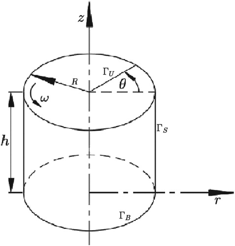
For the description of the flow, the cylindrical coordinates ($\mathit{r}$,θ,$\mathit{z}$) with standard basis ${\mathbf{e}}_r,{\mathbf{e}}_{\theta },{\mathbf{e}}_z$ is employed. Consider a geometry of cylinder with radius R and height h, as shown in Figure 5. Its bottom surface ${\mathrm{\Gamma }}_B$ is fixed while the top surface ${\mathrm{\Gamma }}_U$ is rotating with a given angular speed. The lateral boundary of the cylinder ${\mathrm{\Gamma }}_S$ is traction free. Even though the lateral boundary of the cylinder is free, the inflow and outflow of the fluids are either zero or negligible in the given experiment. Hence, the appropriate boundary conditions are (41) $\begin{array}{ll}\mathbf{v}=\mathbf{0}& \mathrm{on}{\mathrm{\Gamma }}_B,\\ \mathbf{v}=\omega r{\mathbf{e}}_{\theta }& \mathrm{on}{\mathrm{\Gamma }}_U,\\ \mathbf{T}\mathbf{n}=\mathbf{0}& \mathrm{on}{\mathrm{\Gamma }}_S,\end{array}$(41) where $\mathbf{n}$ is the unit outward normal to the boundary ${\mathrm{\Gamma }}_S$.

Figure 5. Geometry of the cylinder for the torsional flow under consideration.

The initial conditions are given by (42) $\mathbf{v}(\mathbf{x},0)=\mathbf{0},{\mathbf{B}}_{\kappa pt}(\mathbf{x},0)=\mathbf{I}.$(42) In this study, the flow is assumed to be axisymmetric, which helps to reduce the computational domain to 2D cross-section. The resultant torque takes the form (43) $M={\int }_0^{R}2\pi r^2{T}_{\theta z}(r,h)\mathrm{d}r.$(43) Based on the experimental observation, the flow of the sample in the radial direction is being neglected. Therefore the velocity field is given by (44) ${\mathbf{v}}_r=0,{\mathbf{v}}_{\theta }=\frac{\omega rz}{h}{\mathbf{e}}_{\theta },{\mathbf{v}}_z=0.$(44) For unsteady flow, the left Cauchy–Green stretch tensor ${\mathbf{B}}_{{\kappa }_{p(t)}}$ is given through (45) ${\mathbf{B}}_{{\kappa }_{p(t)}}=\left(\begin{array}{ccccccc}{B}_{rr}(r,z,t)& B_{r\theta }(r,z,t)& B_{rz}(r,z,t)B_{r\theta }(r,z,t)& B_{\theta \theta }(r,z,t)& B_{\theta z}(r,z,t)B_{rz}(r,z,t)& B_{\theta z}(r,z,t)& B_{zz}(r,z,t)\end{array}\right).$(45) The velocity gradient for this motion is (46) $\mathbf{L}=\left(\begin{array}{ccccccc}0& -{\displaystyle \frac{\omega z}{h}}& 0{\displaystyle \frac{\omega z}{h}}& 0& {\displaystyle \frac{\omega r}{h}}0& 0& 0\end{array}\right).$(46) By substituting Equations (45(45) ${\mathbf{B}}_{{\kappa }_{p(t)}}=\left(\begin{array}{ccccccc}{B}_{rr}(r,z,t)& B_{r\theta }(r,z,t)& B_{rz}(r,z,t)B_{r\theta }(r,z,t)& B_{\theta \theta }(r,z,t)& B_{\theta z}(r,z,t)B_{rz}(r,z,t)& B_{\theta z}(r,z,t)& B_{zz}(r,z,t)\end{array}\right).$(45) ) and (46(46) $\mathbf{L}=\left(\begin{array}{ccccccc}0& -{\displaystyle \frac{\omega z}{h}}& 0{\displaystyle \frac{\omega z}{h}}& 0& {\displaystyle \frac{\omega r}{h}}0& 0& 0\end{array}\right).$(46) ) into Equation (10(10) ${\stackrel{\mathrm{\nabla }}{\mathbf{B}}}_{{\kappa }_{p(t)}}={\dot{\mathbf{B}}}_{{\kappa }_{p(t)}}-\mathbf{L}{\mathbf{B}}_{{\kappa }_{p(t)}}-{\mathbf{B}}_{{\kappa }_{p(t)}}{\mathbf{L}}^{\mathrm{T}}=-2{\mathbf{F}}_{{\kappa }_{p(t)}}{\mathbf{D}}_{{\kappa }_{p(t)}}{\mathbf{F}}_{{\kappa }_{p(t)}}^{\mathrm{T}}.$(10) ), and by using the evolution equation  (37(37) $\sqrt{\mathrm{tr}({\mathbf{B}}_{{\kappa }_{p(t)}})-3\lambda }{\stackrel{\mathrm{\nabla }}{\mathbf{B}}}_{{\kappa }_{p(t)}}=-2\sqrt{{\mathbf{D}}_{{\kappa }_{p(t)}}\cdot {\mathbf{B}}_{{\kappa }_{p(t)}}{\mathbf{D}}_{{\kappa }_{p(t)}}}({\mathbf{B}}_{{\kappa }_{p(t)}}-\lambda \mathbf{I}),$(37) ) one arrives at the following equations: (47) $\begin{array}{rl}\frac{\mathrm{\partial }{B}_{rr}}{\mathrm{\partial }t}& =-2\sqrt{Q}{B}_{rr}+2\sqrt{Q}\lambda ,\\ \frac{\mathrm{\partial }{B}_{r\theta }}{\mathrm{\partial }t}& =-2\sqrt{Q}{B}_{r\theta }+\frac{r\omega }{h}{B}_{rz},\\ \frac{\mathrm{\partial }{B}_{rz}}{\mathrm{\partial }t}& =-2\sqrt{Q}{B}_{rz},\\ \frac{\mathrm{\partial }{B}_{\theta \theta }}{\mathrm{\partial }t}& =-2\sqrt{Q}{B}_{\theta \theta }+\frac{2r\omega }{h}{B}_{\theta z}+2\sqrt{Q}\lambda ,\\ \frac{\mathrm{\partial }{B}_{\theta z}}{\mathrm{\partial }t}& =-2\sqrt{Q}{B}_{\theta z}+\frac{r\omega }{h}{B}_{zz},\\ \frac{\mathrm{\partial }{B}_{zz}}{\mathrm{\partial }t}& =-2\sqrt{Q}{B}_{zz}+2\sqrt{Q}\lambda ,\end{array}$(47) where Q is the solution of Equation (38(38) $Z^2{\beta }^2{Q}^{2\beta -1}={\left(\frac{\mu }{\eta }\right)}^2{[1+\frac{b}{n}(\mathrm{tr}({\mathbf{B}}_{{\kappa }_{p(t)}})-3)]}^{2n-2}(\mathrm{tr}({\mathbf{B}}_{{\kappa }_{p(t)}})-3\lambda {)}^{2-2\beta },$(38) ) and λ is the solution of Equation (32(32) $\lambda =\frac{6}{(\mathrm{tr}({\mathbf{B}}_{{\kappa }_{p(t)}}){)}^2-\mathrm{tr}({\mathbf{B}}_{{\kappa }_{p(t)}}^2)}.$(32) ).

By knowing ${\mathbf{B}}_{\theta z}$, one computes the component of the stress tensor $T_{\theta z}$ using Equation (40(40) $\mathbf{T}=-p\mathbf{I}+Zϵ\gamma (\mathbf{D}\cdot \mathbf{D}{)}^{\gamma -1}\mathbf{D}+\mu {[1+\frac{b}{n}(\mathrm{tr}({\mathbf{B}}_{{\kappa }_{p(t)}})-3)]}^{n-1}{\mathbf{B}}_{{\kappa }_{p(t)}}.$(40) ), (48) $T_{\theta z}=Zϵ\gamma {\left(\frac{r^2{\omega }^2}{2h^2}\right)}^{\gamma }\frac{h}{r\omega }+\mu {[1+\frac{b}{n}(tr{\mathbf{B}}_{{\kappa }_{p(t)}}-3)]}^{n-1}{B}_{\theta z}.$(48) The torque is computed by Equation (43(43) $M={\int }_0^{R}2\pi r^2{T}_{\theta z}(r,h)\mathrm{d}r.$(43) ).

5. Validation of the constitutive equations

To determine the efficacy of the model in predicting the nonlinear response observed from experiments, the effect of shear rate on torque is simulated by using the constitutive equations developed in Section 3.3. It is observed that the initial conditions as well as Equations (47(47) $\begin{array}{rl}\frac{\mathrm{\partial }{B}_{rr}}{\mathrm{\partial }t}& =-2\sqrt{Q}{B}_{rr}+2\sqrt{Q}\lambda ,\\ \frac{\mathrm{\partial }{B}_{r\theta }}{\mathrm{\partial }t}& =-2\sqrt{Q}{B}_{r\theta }+\frac{r\omega }{h}{B}_{rz},\\ \frac{\mathrm{\partial }{B}_{rz}}{\mathrm{\partial }t}& =-2\sqrt{Q}{B}_{rz},\\ \frac{\mathrm{\partial }{B}_{\theta \theta }}{\mathrm{\partial }t}& =-2\sqrt{Q}{B}_{\theta \theta }+\frac{2r\omega }{h}{B}_{\theta z}+2\sqrt{Q}\lambda ,\\ \frac{\mathrm{\partial }{B}_{\theta z}}{\mathrm{\partial }t}& =-2\sqrt{Q}{B}_{\theta z}+\frac{r\omega }{h}{B}_{zz},\\ \frac{\mathrm{\partial }{B}_{zz}}{\mathrm{\partial }t}& =-2\sqrt{Q}{B}_{zz}+2\sqrt{Q}\lambda ,\end{array}$(47) ) are independent of z and therefore, the components of the left Cauchy–Green stretch tensor ${\mathbf{B}}_{{\kappa }_{p(t)}}$ do not depend on this coordinate. Since the components of ${\mathbf{B}}_{{\kappa }_{p(t)}}$ are functions of r and time t, one needs to solve Equations (47(47) $\begin{array}{rl}\frac{\mathrm{\partial }{B}_{rr}}{\mathrm{\partial }t}& =-2\sqrt{Q}{B}_{rr}+2\sqrt{Q}\lambda ,\\ \frac{\mathrm{\partial }{B}_{r\theta }}{\mathrm{\partial }t}& =-2\sqrt{Q}{B}_{r\theta }+\frac{r\omega }{h}{B}_{rz},\\ \frac{\mathrm{\partial }{B}_{rz}}{\mathrm{\partial }t}& =-2\sqrt{Q}{B}_{rz},\\ \frac{\mathrm{\partial }{B}_{\theta \theta }}{\mathrm{\partial }t}& =-2\sqrt{Q}{B}_{\theta \theta }+\frac{2r\omega }{h}{B}_{\theta z}+2\sqrt{Q}\lambda ,\\ \frac{\mathrm{\partial }{B}_{\theta z}}{\mathrm{\partial }t}& =-2\sqrt{Q}{B}_{\theta z}+\frac{r\omega }{h}{B}_{zz},\\ \frac{\mathrm{\partial }{B}_{zz}}{\mathrm{\partial }t}& =-2\sqrt{Q}{B}_{zz}+2\sqrt{Q}\lambda ,\end{array}$(47) ) at each r in between 0 and 12.5 mm. Here, we considered about two hundred equally spaced points between 0 and 12.5 mm, which is sufficient for obtaining accurate results. Simultaneous integration of the differential equations (47(47) $\begin{array}{rl}\frac{\mathrm{\partial }{B}_{rr}}{\mathrm{\partial }t}& =-2\sqrt{Q}{B}_{rr}+2\sqrt{Q}\lambda ,\\ \frac{\mathrm{\partial }{B}_{r\theta }}{\mathrm{\partial }t}& =-2\sqrt{Q}{B}_{r\theta }+\frac{r\omega }{h}{B}_{rz},\\ \frac{\mathrm{\partial }{B}_{rz}}{\mathrm{\partial }t}& =-2\sqrt{Q}{B}_{rz},\\ \frac{\mathrm{\partial }{B}_{\theta \theta }}{\mathrm{\partial }t}& =-2\sqrt{Q}{B}_{\theta \theta }+\frac{2r\omega }{h}{B}_{\theta z}+2\sqrt{Q}\lambda ,\\ \frac{\mathrm{\partial }{B}_{\theta z}}{\mathrm{\partial }t}& =-2\sqrt{Q}{B}_{\theta z}+\frac{r\omega }{h}{B}_{zz},\\ \frac{\mathrm{\partial }{B}_{zz}}{\mathrm{\partial }t}& =-2\sqrt{Q}{B}_{zz}+2\sqrt{Q}\lambda ,\end{array}$(47) ) was performed numerically with a fourth-order Runge–Kutta (RK4) discretization in time. From the knowledge of ${\mathbf{B}}_{\theta z}$, one can compute the model predictions of torque as a function of time.

A heuristic search algorithm referred to as Genetic Algorithm (GA) [29] is used here which is based on Darwin's theory of natural selection. Genetic algorithm begins with a randomly generated population of chromosomes within the bounds of decision variables and executes a process of fitness-based selection and recombination to create a successor population, the next generation. During recombination, parent chromosomes are selected and bred together using genetic operators such as cross-over mating and mutation inspired by natural genetics to produce offsprings. To preserve the best solution, the best chromosomes are taken to the next generation by the process of selection [30]. This then leads to the evolution of the next generation consisting of better offsprings. This procedure is iterated and a sequence of successive generations evolves with average fitness which tends to improve until the stopping criteria (Fitness limit, Stall generations, Function tolerance, etc.) are satisfied. In this manner, a GA ‘evolves’ to find the global optima for a given problem.

Figure 6 shows a flow diagram of the solution methodology used in obtaining an optimal set of model parameters for all the three shear rates. Here, $M_j(t)$ represents the predicted torque corresponding to the jth data point, and $E_j(t)$ represents the measured torque. Genetic Algorithm (GA) optimizes the parameters to minimize the fitness value as depicted in the above flow diagram (see Figure 6). To find an optimal solution, GA creates a large population of parameters over several generations through its iterative procedure. In the above formulation, one inequality constraint has been considered, i.e. $\beta >0.5$ due to the fact that comes from the analogue related to the standard power law fluid model with dissipation in the form $\Vert \mathbf{D}{\Vert }^{2\beta }$. By conducting several trial runs, we were able to gradually find out the following bounds of parameters $(1\times {10}^3\le ϵ\le 5\times {10}^3)$, $(16\times {10}^3\le \eta \le 34\times {10}^3)$, $(0.1\times {10}^3\le \mu \le 1.1\times {10}^3)$, $(0.51\le \gamma \le 0.54)$, $(0.9\le \beta \le 1.5)$, $(16\le b\le 29)$, $(12\le n\le 72)$. The optimized material parameter values are given in Table 2.

Figure 6. Flow diagram of solution methodology for the optimization of model parameters.

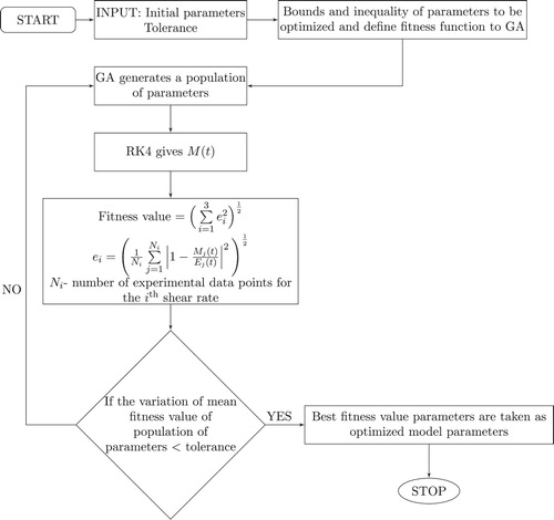
Table 2. Optimized values associated with the parameters of the model.

Samples	$ϵ[{10}^3\mathrm{Pa}{\mathrm{s}}^{2\gamma -1}]$	$\eta [{10}^3\mathrm{Pa}{\mathrm{s}}^{2\beta -1}]$	$\mu [{10}^3\mathrm{Pa}]$	γ	β	b	n
S1	1.16	18.96	0.316	0.52	1.3	26	28
S2	4.49	32.96	0.826	0.51	1.2	26	66

Note: S1 – samples with a shear strength of approximately 1 kPa; S2 – samples with a shear strength of approximately 3 kPa.

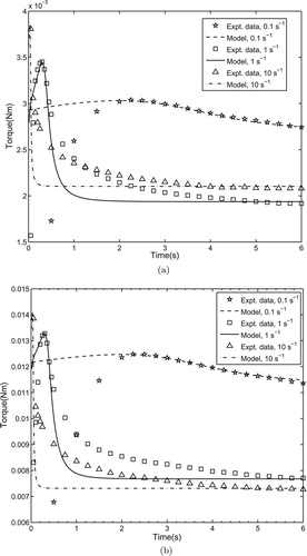
Figure 7 shows the variation of experimental and the predicted torque with respect to time for various shear rates. It can be seen that the model is better suited to describe the qualitative response observed in the experimental data on two selected samples having different shear strength. With one set of parameters, the model is able to capture the peak as well as steady-state values of torque over a wide range of shear rates ranging from 0.1 to $10{\mathrm{s}}^{-1}$. It transpired that the developed model established its proficiency in predicting the long-term behaviour of material media which solely depends on the steady-state values. Recall that a simple form equation (19(19) $\psi =\frac{\mu }{2\rho b}\{{[1+\frac{b}{n}(\mathrm{tr}({\mathbf{B}}_{{\kappa }_{p(t)}})-3)]}^n-1\},$(19) ) for Helmholtz potential with just three parameters is adopted here. By selecting a different functional form with more number of parameters, one can obtain a more accurate prediction.

Figure 7. Comparison of the torque predicted by the model with that of the experimental data at various shear rates: (a) sample with shear strength of 1 kPa and (b) sample with shear strength of 3 kPa.

6. Conclusions

In this paper, the nonlinear viscoelastic behaviour of deep-seabed sediments has been illustrated based on the shear rheological test conducted on two selected simulative soil (bentonite-water mixture) samples at different values of shear rates. The results of the experiments clearly show that the response of the samples is nonlinear. The interesting feature observed from the experiment is that the peak as well as steady-state values of torque are affected by shear rate and water content. A nonlinear viscoelastic fluid model based on a general thermodynamic framework is derived to simulate the responses observed from experiments. The model is based on two scalar functions, namely, the stored energy and rate of dissipation functions which are deduced by making suitable assumptions concerning the manner in which the simulative soil stores and dissipates energy. The parameters associated with the model are determined by the minimization of error function between the measured and predicted torque using GA. The model parameters have a physical significance, in contrast to the other predominantly empirical models for deep-sea sediments where the parameters vary with the type of testing. Thus, with one set of the material moduli, the developed model is able to capture the peak as well as steady-state values of torque observed in the experimental data over a wide range of shear rates ranging from 0.1 to $10{\mathrm{s}}^{-1}$. This is of great importance since the steady-state values are used in describing the long-term behaviour of material media. It is very likely that this study will serve as an initial step towards another type of experiments and for different types of samples with various shear strength. This work provides a detailed methodology about the identification of parameters for the sea bed sediments using two scalar functions which leaves a significant scope for further research to develop better constitutive equations.

Disclosure statement

No potential conflict of interest was reported by the authors.

ORCID

K. Kannan  http://orcid.org/0000-0002-9337-3046

S. Sumith  http://orcid.org/0000-0003-0196-0882

Additional information

Funding

The authors gratefully acknowledge the support and funding of this study by the National Institute of Ocean Technology (NIOT), Government of India.

References

- Kato Y, Fujinaga K, Nakamura K, et al. Deep-sea mud in the Pacific Ocean as a potential resource for rare-earth elements. Nat Geosci. 2011;4(8):535–539. doi: 10.1038/ngeo1185
- Hong S, Kim HW, Choi JS, et al. Transient dynamic analysis of tracked vehicles on extremely soft cohesive soil. The Fifth ISOPE Pacific/Asia Offshore Mechanics Symposium; International Society of Offshore and Polar Engineers; Nov 17--20; Daejeon, Korea; 2002. p. 100–107.
- Dai Y, Liu SJ. Theoretical design and dynamic simulation of new mining paths of tracked miner on deep seafloor. J Central South Univ. 2013;20(4):918–923. doi: 10.1007/s11771-013-1566-z
- Brandes HG. Geotechnical characteristics of deep-sea sediments from the North Atlantic and North Pacific oceans. Ocean Eng. 2011;38(7):835–848. doi: 10.1016/j.oceaneng.2010.09.001
- Kim HW, Hong S, Choi JS, et al. An experimental study on tractive performance of tracked vehicle on cohesive soft soil. Fifth ISOPE Ocean Mining Symposium; International Society of Offshore and Polar Engineers; Sep 15--19; Tsukuba, Japan; 2003. p. 139–143.
- Schulte E, Schwarz W. Simulation of tracked vehicle performance on deep sea soil based on soil mechanical laboratory measurements in bentonite soil. Eighth ISOPE Ocean Mining Symposium; International Society of Offshore and Polar Engineers; Sep 20--24; Chennai, India; 2009. p. 276–284.
- Ma Wb, Rao Qh, Li P, et al. Shear creep parameters of simulative soil for deep-sea sediment. J Central South Univ. 2014;21(12):4682–4689. doi: 10.1007/s11771-014-2477-3
- Schulte E, Handschuh R, Schwarz W, et al. Transferability of soil mechanical parameters to traction potential calculation of a tracked vehicle. Fifth ISOPE Ocean Mining Symposium; International Society of Offshore and Polar Engineers; Sep 15--19; Tsukuba, Japan; 2003. p. 123–131.
- Wu H, He J, Chen X, et al. Establishment of the deep-sea soft sediments shearing strength-shearing displacement model. Mod Appl Sci. 2010;4(1):21–27.
- Wang M, Wu C, Ge T, et al. Modeling, calibration and validation of tractive performance for seafloor tracked trencher. J Terramech. 2016;66:13–25. doi: 10.1016/j.jterra.2016.03.001
- Mainardi F, Spada G. Creep, relaxation and viscosity properties for basic fractional models in rheology. Eur Phys J Spec Top. 2011;193(1):133–160. doi: 10.1140/epjst/e2011-01387-1
- Xu F, Rao QH, Zhang J, et al. Compression–shear coupling rheological constitutive model of the deep-sea sediment. Mar Georesour Geotechnol. 2018;36(3):288–296. doi: 10.1080/1064119X.2017.1286530
- Kelessidis V. Investigations on the thixotropy of bentonite suspensions. Energy Sources Part A. 2008;30(18):1729–1746. doi: 10.1080/15567030701456261
- Barnes HA. Thixotropy – a review. J Non-Newton Fluid Mech. 1997;70(1–2):1–33. doi: 10.1016/S0377-0257(97)00004-9
- Alderman N, Meeten G, Sherwood J. Vane rheometry of bentonite gels. J Non-Newton Fluid Mech. 1991;39(3):291–310. doi: 10.1016/0377-0257(91)80019-G
- Heller H, Keren R. Rheology of na-rich montmorillonite suspension as affected by electrolyte concentration and shear rate. Clays Clay Miner. 2001;49(4):286–291. doi: 10.1346/CCMN.2001.0490402
- Bekkour K, Leyama M, Benchabane A, et al. Time-dependent rheological behavior of bentonite suspensions: an experimental study. J Rheol. 2005;49(6):1329–1345. doi: 10.1122/1.2079267
- Bekkour K, Kherfellah N. Linear viscoelastic behavior of bentonite-water suspensions. Appl Rheol. 2002;12(5):234–240. doi: 10.1515/arh-2002-0012
- Rajagopal K, Srinivasa A. A thermodynamic frame work for rate type fluid models. J Non-Newton Fluid Mech. 2000;88(3):207–227. doi: 10.1016/S0377-0257(99)00023-3
- Choi JS, Hong S, Chi SB, et al. Probability distribution for the shear strength of seafloor sediment in the KR5 area for the development of manganese nodule miner. Ocean Eng. 2011;38(17–18):2033–2041. doi: 10.1016/j.oceaneng.2011.09.011
- Babu SM, Ramesh N, Muthuvel P, et al. In-situ soil testing in the central Indian Ocean basin at 5462-m water depth. Tenth ISOPE Ocean Mining and Gas Hydrates Symposium; International Society of Offshore and Polar Engineers; Sep 22--26; Szczecin, Poland; 2013. p. 190–197.
- Benna M, Kbir-Ariguib N, Magnin A, et al. Effect of ph on rheological properties of purified sodium bentonite suspensions. J Colloid Interface Sci. 1999;218(2):442–455. doi: 10.1006/jcis.1999.6420
- Chhabra RP, Richardson JF. Non-Newtonian flow and applied rheology: engineering applications. Amsterdam: Butterworth-Heinemann; 2011.
- Málek J, Rajagopal KR. Incompressible rate type fluids with pressure and shear-rate dependent material moduli. Nonlinear Anal: Real World Appl. 2007;8(1):156–164. doi: 10.1016/j.nonrwa.2005.06.006
- Malek J, Rajagopal KR, Tuma K. On a variant of the Maxwell and Oldroyd-B models within the context of a thermodynamic basis. Int J Non-Linear Mech. 2015;76:42–47. doi: 10.1016/j.ijnonlinmec.2015.03.009
- Hron J, Kratochvil J, Malek J, et al. A thermodynamically compatible rate type fluid to describe the response of asphalt. Math Comput Simul. 2012;82(10):1853–1873. doi: 10.1016/j.matcom.2011.03.010
- Monigari K, Kannan K. A class of models to predict the normal force and torque under torsional loading of a viscoelastic liquid. Int J Eng Sci. 2013;71:80–91. doi: 10.1016/j.ijengsci.2013.06.003
- Suchocki C. A finite element implementation of knowles stored-energy function: theory, coding and applications. Arch Mech Eng. 2011;58(3):319–346. doi: 10.2478/v10180-011-0021-7
- Mitchell M. An introduction to genetic algorithms. Cambridge (MA): MIT Press; 1998.
- Beasley D, Bull DR, Martin RR. An overview of genetic algorithms: part 1, fundamentals. Univ Comput. 1993;15(2):56–69.