On the choice of Lagrange multipliers in the iterated Tikhonov method for linear ill-posed equations in Banach spaces

ABSTRACT

This article is devoted to the study of nonstationary Iterated Tikhonov (nIT) type methods (Hanke M, Groetsch CW. Nonstationary iterated Tikhonov regularization. J Optim Theory Appl. 1998;98(1):37–53; Engl HW, Hanke M, Neubauer A. Regularization of inverse problems. Vol. 375, Mathematics and its Applications. Dordrecht: Kluwer Academic Publishers Group; 1996. MR 1408680) for obtaining stable approximations to linear ill-posed problems modelled by operators mapping between Banach spaces. Here we propose and analyse an a posteriori strategy for choosing the sequence of regularization parameters for the nIT method, aiming to obtain a pre-defined decay rate of the residual. Convergence analysis of the proposed nIT type method is provided (convergence, stability and semi-convergence results). Moreover, in order to test the method's efficiency, numerical experiments for three distinct applications are conducted: (i) a 1D convolution problem (smooth Tikhonov functional and Banach parameter-space); (ii) a 2D deblurring problem (nonsmooth Tikhonov functional and Hilbert parameter-space); (iii) a 2D elliptic inverse potential problem.

KEYWORDS:

• Ill-posed problems
• Banach spaces
• linear operators
• iterated Tikhonov method

2010 MATHEMATICS SUBJECT CLASSIFICATIONS:

• 65J20
• 47J06

1. Introduction

In this article we investigate nonstationary Iterated Tikhonov (nIT) type methods [1,2] for obtaining stable approximations of linear ill-posed problems modelled by operators mapping between Banach spaces. The novelty of our approach consists in the introduction of an a posteriori strategy for choosing the sequence of regularization parameters (or, equivalently, the Lagrange multipliers) for the nIT iteration, which play a key role in the convergence speed of the nIT iteration.

This new a posteriori strategy aims to enforce a pre-defined decay of the residual in each iteration; it differs from the classical choice for the Lagrange multipliers (see, e.g. [2,3]), which is based on an a priori strategy (typically geometrical) and leads to an unknown decay rate of the residual.

The inverse problem we are interested in consists of determining an unknown quantity $x\in X$ from given data $y\in Y$, where X, Y are Banach spaces. We assume that data are obtained by indirect measurements of the parameter, this process being described by the ill-posed operator equation (1) $Ax=y,$(1) where $A:X\to Y$ is a bounded linear operator, whose inverse $A^{-1}:R(A)\to X$ either does not exist, or is not continuous. In practical situations, one does not know the data y exactly; instead, only approximate measured data $y^{\delta }\in Y$ are available with (2) $\Vert y^{\delta }-y{\Vert }_Y\le \delta ,$(2) where $\delta >0$ is the (known) noise level. A comprehensive study of linear ill-posed problems in Banach spaces can be found in the text book [4] (see, e.g. [1] for a corresponding theory in Hilbert spaces).

Iterated Tikhonov type methods are typically used for linear inverse problems. In the Hilbert space setting we refer the reader to [2] for linear operator equations, and also to [5] for the nonlinear case. In the Banach space setting the research is still ongoing. Some preliminary results can be found in [3] for linear operator equations; see [6] for the nonlinear case; see also [7]. In all references above, a priori strategies are used for choosing the Lagrange multipliers.

1.1. Main results: presentation and interpretation

The approach discussed in this manuscript is devoted to the Banach space setting, and consists in adopting an a posteriori strategy for the choice of the Lagrange multipliers. The strategy used here is inspired by the recent work [8], where the authors propose an endogenous strategy for the choice of the Lagrange multipliers in the nonstationary iterated Tikhonov method for solving (1(1) $Ax=y,$(1) ), (2(2) $\Vert y^{\delta }-y{\Vert }_Y\le \delta ,$(2) ) when X and Y are Hilbert spaces. The penalty terms used in our Tikhonov functionals are the same as in [6] and consist of Bregman distances induced by (uniformly) convex functionals, e.g. the sum of the $L^2$-norm with the TV -seminorm. In our previous work [9], we implemented the method proposed in this paper and investigated its numerical performance (two different ill-posed problems were solved). Here, we extend our previous results by presenting a whole convergence analysis. Additionally, the corresponding algorithm is implemented for solving three benchmark problems and more details concerning the computation of the minimizers of the Tikhonov functional are provided; our numerical results are compared with the ones obtained using the nIT method using the classical geometrical choice of Lagrange multipliers [6].

In what follows, we briefly interpret the main results: The proposed method defines each Lagrange multiplier such that the residual of the corresponding next iterate lies in an interval which depends on both the noise level and the residual of the current iterate (see (23(23) $[(1-{\eta }_0)\delta +{\eta }_0\Vert A{x}_k^{\delta }-y^{\delta }\Vert ,(1-{\eta }_1)\delta +{\eta }_1\Vert A{x}_k^{\delta }-y^{\delta }\Vert ].$(23) )). This fact has the following consequences: (1) it forces a geometrical decay of the residual (Proposition 4.1); (2) it guarantees the possibility of computing multipliers in agreement with the theoretical convergence results (Theorems 4.6, 4.8 and 4.9); (3) the computation of the multipliers demands less numerical effort than the classical strategy of computing the multipliers by solving an equation in each iteration; (4) the next iterate is not uniquely determined by the current one; instead, it is chosen within a set of successors of the current iterate (Definition 4.7). We also address the actual computation of the Lagrange multipliers. Since each multiplier is implicitly defined by an inequality, we discuss a numerically efficient strategy for computing them, which is based on the decrease rate of the past residuals (Section 5.1).

1.2. Outline of the article

This manuscript is outlined as follows: In Section 2 a revision of relevant background material is presented. In Section 3 the new nIT method is introduced. Section 4 is devoted to the convergence analysis of the nIT method. In Section 5 possible implementations of our method are discussed; the evaluation of the Lagrange multipliers is addressed, as well as the issue of minimizing the Tikhonov functionals. Section 6 is devoted to numerical experiments, while Section 7 is dedicated to final remarks and conclusions.

2. Background material

For details on the material discussed in this section, we refer the reader to the textbooks [4,10].

Unless the contrary is explicitly stated, we always consider X a real Banach space. The effective domain of the convex functional $f:X\to \overline{\mathbb{R}}:=(-\mathrm{\infty },\mathrm{\infty }]$ is defined as $\mathrm{Dom}\left(f\right):=\{x\in X:f\left(x\right)<\mathrm{\infty }\}.$ The set $\mathrm{Dom}(f)$ is always convex and we call f proper provided it is non-empty. We call f uniformly convex if there exists a continuous and strictly increasing function $\phi :{\mathbb{R}}_0^{+}\to {\mathbb{R}}_0^{+}$ with the property $\phi (t)=0$ implies $t=0,$ such that (3) $f(\lambda x+(1-\lambda )y)+\lambda (1-\lambda )\phi \left(\Vert x-y\Vert \right)\le \lambda f\left(x\right)+(1-\lambda )f\left(y\right),$(3) for all $\lambda \in (0,1)$ and $x,y\in X.$ Of course f uniformly convex implies f strictly convex, which in turn implies f convex. The functional f is lower semi-continuous (in short l.s.c.) if for any sequence $(x_k{)}_{k\in \mathbb{N}}\subset X$ satisfying $x_k\to x$, it holds $f\left(x\right)\le lim\underset{k\to \mathrm{\infty }}{inf}f\left(x_k\right).$ It is called weakly lower semi-continuous (w.l.s.c.) if above property holds true with $x_k\to x$ replaced by $x_k\rightharpoonup x.$ Obviously, every w.l.s.c functional is l.s.c. Further, any Banach space norm is w.l.s.c.

The sub-differential of a functional $f:X\to \overline{\mathbb{R}}$ is the point-to-set mapping $\mathrm{\partial }f:X\to 2^{X^{\ast }}$ defined by $\mathrm{\partial }f\left(x\right):=\{x^{\ast }\in X^{\ast }:f\left(x\right)+⟨x^{\ast },y-x⟩\le f\left(y\right)\mathrm{for}\mathrm{all}y\in X\}.$ Any element in the set $\mathrm{\partial }f(x)$ is called a sub-gradient of f at x. The effective domain of $\mathrm{\partial }f$ is the set $\mathrm{Dom}\left(\mathrm{\partial }f\right):=\{x\in X:\mathrm{\partial }f\left(x\right)\ne \mathrm{\varnothing }\}.$ It is clear that the inclusion $\mathrm{Dom}(\mathrm{\partial }f)\subset \mathrm{Dom}(f)$ holds whenever f is proper.

Sub-differentiable functionals and l.s.c. convex functionals are very close related concepts. In fact, a sub-differentiable functional f is convex and l.s.c. in any open convex set of $\mathrm{Dom}(f).$ On the other hand, a proper, convex and l.s.c. functional is always sub-differentiable on its effective domain.

The definition of sub-differential readily yields $0\in \mathrm{\partial }f\left(x\right)⟺f\left(x\right)\le f\left(y\right)\mathrm{for}\mathrm{all}y\in X.$ If $f,g:X\to \overline{\mathbb{R}}$ are convex functionals and there is a point $x\in \mathrm{Dom}(f)\cap \mathrm{Dom}(g)$ where f is continuous, then (4) $\mathrm{\partial }(f+g)\left(x\right)=\mathrm{\partial }f\left(x\right)+\mathrm{\partial }g\left(x\right)\mathrm{for}\mathrm{all}x\in X.$(4) Moreover, if Y is a real Banach space, $h:Y\to \overline{\mathbb{R}}$ is a convex functional, $b\in Y,$ $A:X\to Y$ is a bounded linear operator and h is continuous at some point of the range of A, then $\mathrm{\partial }\left(h(\cdot -b)\right)\left(y\right)=\left(\mathrm{\partial }h\right)(y-b)\mathrm{and}\mathrm{\partial }(h\circ A)\left(x\right)=A^{\ast }\left(\mathrm{\partial }h\left(Ax\right)\right),$ for all $x\in X$ and $y\in Y,$ where $A^{\ast }:Y^{\ast }\to X^{\ast }$ is the Banach-adjoint of A. Consequently, (5) $\mathrm{\partial }\left(h(A\cdot -b)\right)\left(x\right)=A^{\ast }\left(\mathrm{\partial }h\right)(Ax-b)\mathrm{for}\mathrm{all}x\in X.$(5) If a convex functional $f:X\to \overline{\mathbb{R}}$ is Gâteaux-differentiable at $x\in X,$ then f has a unique sub-gradient at x, namely, the Gâteaux-derivative itself: $\mathrm{\partial }f(x)=\{\mathrm{\nabla }f(x)\}.$

The sub-differential of the convex functional (6) $f\left(x\right)=\frac{1}{p}{\Vert x\Vert }^p,p>1,$(6) is called the duality mapping and is denoted by $J_p.$ It can be shown that for all $x\in X,$ $J_p\left(x\right)=\{x^{\ast }\in X^{\ast }:⟨x^{\ast },x⟩=\Vert x^{\ast }\Vert \Vert x\Vert \mathrm{and}\Vert x^{\ast }\Vert ={\Vert x\Vert }^{p-1}\}.$ Thus, the duality mapping has the inner-product-like properties: $⟨x^{\ast },y⟩\le {\Vert x\Vert }^{p-1}\Vert y\Vert \mathrm{and}⟨x^{\ast },x⟩={\Vert x\Vert }^p,$ for all $x^{\ast }\in J_p(x).$ By using the Riesz Representation Theorem, one can prove that $J_2(x)=x$ for all $x\in X$ whenever X is a Hilbert space.

Banach spaces are classified according with their geometrical characteristics. Many concepts concerning these characteristics are usually defined using the so called modulus of convexity and modulus of smoothness, but most of these definitions can be equivalently stated observing the properties of the functional f defined in (6(6) $f\left(x\right)=\frac{1}{p}{\Vert x\Vert }^p,p>1,$(6) ).¹ This functional is convex and sub-differentiable in any Banach space X. If (6(6) $f\left(x\right)=\frac{1}{p}{\Vert x\Vert }^p,p>1,$(6) ) is Gâteaux-differentiable in the whole space X, this Banach space is called smooth. In this case, $J_p(x)=\mathrm{\partial }f(x)=\{\mathrm{\nabla }f(x)\}$ and therefore, the duality mapping $J_p:X\to X^{\ast }$ is single-valued. If the functional f in (6(6) $f\left(x\right)=\frac{1}{p}{\Vert x\Vert }^p,p>1,$(6) ) is Fré chet-differentiable in X, this space is called locally uniformly smooth and it is called uniformly smooth provided f is uniformly Fréchet-differentiable in bounded sets. As a result, the duality mapping is continuous (resp. uniformly continuous in bounded sets) in locally uniformly smooth (resp. uniformly smooth) spaces. It is immediate that uniform smoothness of a Banach space implies local uniform smoothness, which in turn implies smoothness of this space. Moreover, none reciprocal is true. Similarly, a Banach space X is called strictly convex whenever (6(6) $f\left(x\right)=\frac{1}{p}{\Vert x\Vert }^p,p>1,$(6) ) is a strictly convex functional. Moreover, X is called uniformly convex if the functional f in (6(6) $f\left(x\right)=\frac{1}{p}{\Vert x\Vert }^p,p>1,$(6) ) is uniformly convex. It is clear that uniform convexity implies strict convexity. It is well-known that both uniformly smooth and uniformly convex Banach spaces are reflexive.

Assume f is proper. Then, choosing elements $x,y\in X$ with $y\in \mathrm{Dom}(\mathrm{\partial }f),$ we define the Bregman distance between x and y in the direction of $\xi \in \mathrm{\partial }f(y)$ as $D_{\xi }f(x,y):=f\left(x\right)-f\left(y\right)-⟨\xi ,x-y⟩.$ Obviously, $D_{\xi }f(y,y)=0$ and, since $\xi \in \mathrm{\partial }f(y),$ it additionally holds that $D_{\xi }f(x,y)\ge 0.$ Moreover, it is straightforward proving the Three Points Identity: $D_{{\xi }_1}f(x_2,x_1)-D_{{\xi }_1}f(x_3,x_1)=D_{{\xi }_3}f(x_2,x_3)+⟨{\xi }_3-{\xi }_1,x_2-x_3⟩,$ for all $x_2\in X,$ $x_1,x_3\in \mathrm{Dom}(\mathrm{\partial }f),$ ${\xi }_1\in \mathrm{\partial }f(x_1)$ and ${\xi }_3\in \mathrm{\partial }f(x_3).$ Further, the functional $D_{\xi }f(\cdot ,y)$ is strictly convex whenever f is strictly convex, and in this case, $D_{\xi }f(x,y)=0$ iff $x=y.$

When f is the functional defined in (6(6) $f\left(x\right)=\frac{1}{p}{\Vert x\Vert }^p,p>1,$(6) ) and X is a smooth Banach space, the Bregman distance has the special notation ${\mathrm{\Delta }}_p(x,y),$ i.e. ${\mathrm{\Delta }}_p(x,y):=\frac{1}{p}{\Vert x\Vert }^p-\frac{1}{p}{\Vert y\Vert }^p-⟨J_p\left(y\right),x-y⟩.$ Since $J_2$ is the identity operator in Hilbert spaces, a simple application of the polarization identity shows that ${\mathrm{\Delta }}_2(x,y)=\frac{1}{2}\Vert x-y{\Vert }^2$ in these spaces.

It is not difficult to prove (see e.g. [9]) that if $f:X\to \overline{\mathbb{R}}$ is uniformly convex, then (7) $\phi \left(\Vert x-y\Vert \right)\le D_{\xi }f(x,y)$(7) for all $x\in X,$ $y\in \mathrm{Dom}(\mathrm{\partial }f)$ and $\xi \in \mathrm{\partial }f(y),$ where ϕ is the function in (3(3) $f(\lambda x+(1-\lambda )y)+\lambda (1-\lambda )\phi \left(\Vert x-y\Vert \right)\le \lambda f\left(x\right)+(1-\lambda )f\left(y\right),$(3) ). In particular, in a smooth and uniformly convex Banach space X, the above inequality reads $\phi (\Vert x-y\Vert )\le {\mathrm{\Delta }}_p(x,y).$

We say that a functional $f:X\to \overline{\mathbb{R}}$ has the Kadec property if for any sequence $(x_k{)}_{k\in \mathbb{N}}\subset X,$ the weak convergence $x_k\rightharpoonup x$, together with $f(x_k)\to f(x)<\mathrm{\infty }$, implies $x_k\to x.$ It is not difficult to prove (see e.g. [6]) that any proper, w.l.s.c. and uniformly convex functional has the Kadec property. In particular, the norm in a uniformly convex Banach space has this property.

Concrete examples of Banach spaces of interest are the Lebesgue space $L^p(\mathrm{\Omega }),$ the Sobolev space $W^{n,p}(\mathrm{\Omega }),$ $n\in \mathbb{N},$ and the space of $p-$summable sequences ${\ell }^p(\mathbb{R}).$ All these Banach spaces are both uniformly convex and uniformly smooth provided that $1<p<\mathrm{\infty }$.

3. The nIT method

In this section, we present the nonstationary iterated Tikhonov (nIT) type method considered in this article, which aims to find stable approximate solutions to the inverse problem (1(1) $Ax=y,$(1) ), (2(2) $\Vert y^{\delta }-y{\Vert }_Y\le \delta ,$(2) ). The method proposed here is in the spirit of the method in [6]. The distinguishing feature is the use of an a posteriori strategy for the choice of the Lagrange multipliers, as detailed below.

For a fixed r>1 and a uniformly convex penalty term f, the nIT method defines sequences $(x_k^{\delta }{)}_{k\in \mathbb{N}}$ in X and $({\xi }_k^{\delta }{)}_{k\in \mathbb{N}}$ in $X^{\ast }$ iteratively by $\begin{array}{rl}& x_k^{\delta }:=\arg \underset{x\in X}{min}{\lambda }_k^{\delta }{r}^{-1}{\Vert Ax-y^{\delta }\Vert }^r+D_{{\xi }_{k-1}^{\delta }}f(x,x_{k-1}^{\delta }),\\ & {\xi }_k^{\delta }:={\xi }_{k-1}^{\delta }-{\lambda }_k^{\delta }{A}^{\ast }{J}_r(A{x}_k^{\delta }-y^{\delta }),\end{array}$ where the Lagrange multiplier ${\lambda }_k^{\delta }>0$ is to be determined using only information about A, δ, $y^{\delta }$ and $x_{k-1}^{\delta }$.

Our strategy for choosing the Lagrange multipliers is inspired by the work [8], where the authors propose an endogenous strategy for the choice of the Lagrange multipliers in the nonsationary iterated Tikhonov method for solving (1(1) $Ax=y,$(1) ), (2(2) $\Vert y^{\delta }-y{\Vert }_Y\le \delta ,$(2) ) when X and Y are Hilbert spaces. This method is based on successive orthogonal projection methods onto a family of shrinking, separating convex sets. Specifically, the iterative method in [8] obtains the new iterate projecting the current one onto a levelset of the residual function, whose level belongs to a range defined by the current residual and by the noise level. Moreover, the admissible Lagrange multipliers (in each iteration) shall be chosen in a non-degenerate interval.

Aiming to extend this framework to the Banach space setting, we are forced to introduce Bregman distance and Bregman projections. This is due to the well-known fact that in Banach spaces the metric projection onto a convex and closed set C, defined as $P_C(x)=argmi{n}_{z\in C}\Vert z-x{\Vert }^2$, loses the decreasing distance property of the orthogonal projection in Hilbert spaces. In order to recover this property, one should minimize in Banach spaces the Bregman distance, instead of the norm-induced distance.

For the remaining of this article we adopt the following main assumptions:

1. There exists an element $x^{\star }\in X$ such that $A{x}^{\star }=y$, where $y\in R(A)$ is the exact data.

2. f is a w.l.s.c. function.

3. f is a uniformly convex function.

4. X and Y are reflexive Banach spaces and Y is smooth.

Moreover, we denote by ${\mathrm{\Omega }}_{\mu }^r\subset X$ the μ-levelset of the residual functional $\Vert Ax-y^{\delta }\Vert$, i.e. ${\mathrm{\Omega }}_{\mu }^r:=\{x\in X:r^{-1}\Vert Ax-y^{\delta }{\Vert }^r\le r^{-1}{\mu }^r\}.$ Note that, since A is a continuous linear operator, it follows that ${\mathrm{\Omega }}_{\mu }^r$ is closed and convex. Now, given $\hat{x}\in \mathrm{Dom}(\mathrm{\partial }f)$ and $\xi \in \mathrm{\partial }f(\hat{x})$, we define the Bregman projection of $\hat{x}$ onto ${\mathrm{\Omega }}_{\mu }^r$, as a solution of the minimization problem (8) $\{\begin{array}{l}min{D}_{\xi }f(x,\hat{x})\\ \mathrm{s}.\mathrm{t}.r^{-1}\Vert Ax-y^{\delta }{\Vert }^r\le r^{-1}{\mu }^r.\end{array}$(8) It is worth noticing that a solution of the problem (8(8) $\{\begin{array}{l}min{D}_{\xi }f(x,\hat{x})\\ \mathrm{s}.\mathrm{t}.r^{-1}\Vert Ax-y^{\delta }{\Vert }^r\le r^{-1}{\mu }^r.\end{array}$(8) ) depends on the sub-gradient ξ. Furthermore, since $D_{\xi }f(\cdot ,\hat{x})$ is strictly convex (which follows from the uniformly convexity of f), problem (8(8) $\{\begin{array}{l}min{D}_{\xi }f(x,\hat{x})\\ \mathrm{s}.\mathrm{t}.r^{-1}\Vert Ax-y^{\delta }{\Vert }^r\le r^{-1}{\mu }^r.\end{array}$(8) ) has at most one solution. The fact that the Bregman projection is well defined when $\mu >\delta$ (in this case we set $P_{{\mathrm{\Omega }}_{\mu }^r}^f(\hat{x}):=\arg \underset{x\in {\mathrm{\Omega }}_{\mu }^r}{min}{D}_{\xi }f(x,\hat{x})$) is a consequence of the following lemma.

Lemma 3.1

If $\mu >\delta ,$ then problem (8(8) $\{\begin{array}{l}min{D}_{\xi }f(x,\hat{x})\\ \mathrm{s}.\mathrm{t}.r^{-1}\Vert Ax-y^{\delta }{\Vert }^r\le r^{-1}{\mu }^r.\end{array}$(8) ) has a solution.

Proof.

Assumption (A.1), together with equation (2(2) $\Vert y^{\delta }-y{\Vert }_Y\le \delta ,$(2) ) and the assumption that $\mu >\delta$, implies that the feasible set of problem (8(8) $\{\begin{array}{l}min{D}_{\xi }f(x,\hat{x})\\ \mathrm{s}.\mathrm{t}.r^{-1}\Vert Ax-y^{\delta }{\Vert }^r\le r^{-1}{\mu }^r.\end{array}$(8) ), i.e. the set ${\mathrm{\Omega }}_{\mu }^r,$ is nonempty.

From Assumptions (A.2) and (A.3) it follows that $D_{\xi }f(\cdot ,\hat{x})$ is proper, convex and l.s.c. Furthermore, relation (7(7) $\phi \left(\Vert x-y\Vert \right)\le D_{\xi }f(x,y)$(7) ) implies that $D_{\xi }f(\cdot ,\hat{x})$ is a coercive function. Hence, the lemma follows using the reflexivity of X together with [11, Corollary 3.23].²

Note that if $0\le {\mu }^{\prime }\le \mu$, then ${\mathrm{\Omega }}_{{\mu }^{\prime }}^r\subseteq {\mathrm{\Omega }}_{\mu }^r$ and $A^{-1}(y)\subset {\mathrm{\Omega }}_{\mu }^r$ for all $\mu \ge \delta$. Furthermore, with the available information of the solution set of (1(1) $Ax=y,$(1) ), ${\mathrm{\Omega }}_{\delta }^r$ is the set of best possible approximate solution for this inverse problem. However, since problem (8(8) $\{\begin{array}{l}min{D}_{\xi }f(x,\hat{x})\\ \mathrm{s}.\mathrm{t}.r^{-1}\Vert Ax-y^{\delta }{\Vert }^r\le r^{-1}{\mu }^r.\end{array}$(8) ) may be ill-posed when $\mu =\delta$, our best choice is to generate $x_k^{\delta }$ from $x_{k-1}^{\delta }\notin {\mathrm{\Omega }}_{\delta }^r$ as a solution of problem (8(8) $\{\begin{array}{l}min{D}_{\xi }f(x,\hat{x})\\ \mathrm{s}.\mathrm{t}.r^{-1}\Vert Ax-y^{\delta }{\Vert }^r\le r^{-1}{\mu }^r.\end{array}$(8) ), with $\hat{x}=x_{k-1}^{\delta }$ and $\mu ={\mu }_k$ such that we guarantee a reduction of the residual norm while preventing ill-posedness of (8(8) $\{\begin{array}{l}min{D}_{\xi }f(x,\hat{x})\\ \mathrm{s}.\mathrm{t}.r^{-1}\Vert Ax-y^{\delta }{\Vert }^r\le r^{-1}{\mu }^r.\end{array}$(8) ).

For this purpose, we analyse in the sequel the minimization problem (8(8) $\{\begin{array}{l}min{D}_{\xi }f(x,\hat{x})\\ \mathrm{s}.\mathrm{t}.r^{-1}\Vert Ax-y^{\delta }{\Vert }^r\le r^{-1}{\mu }^r.\end{array}$(8) ) by means of Lagrange multipliers. The Lagrangian function associated to problem (8(8) $\{\begin{array}{l}min{D}_{\xi }f(x,\hat{x})\\ \mathrm{s}.\mathrm{t}.r^{-1}\Vert Ax-y^{\delta }{\Vert }^r\le r^{-1}{\mu }^r.\end{array}$(8) ) is $\mathcal{L}(x,\lambda )=\frac{\lambda }{r}(\Vert Ax-y^{\delta }{\Vert }^r-{\mu }^r)+D_{\xi }f(x,\hat{x}).$ Note that, for each $\lambda >0$, the function $\mathcal{L}(\cdot ,\lambda ):X\to \overline{\mathbb{R}}$ is l.s.c. and convex. For any $\lambda >0$ define the functions (9) $\pi (\hat{x},\lambda ):=\arg \underset{x\in X}{min}\mathcal{L}(x,\lambda ),G_{\hat{x}}(\lambda ):=\Vert A\pi (\hat{x},\lambda )-y^{\delta }{\Vert }^r.$(9) The next lemma provides a classical Lagrange multiplier result for problem (8(8) $\{\begin{array}{l}min{D}_{\xi }f(x,\hat{x})\\ \mathrm{s}.\mathrm{t}.r^{-1}\Vert Ax-y^{\delta }{\Vert }^r\le r^{-1}{\mu }^r.\end{array}$(8) ), which will be useful for formulating the nIT method.

Lemma 3.2

If $\Vert A\hat{x}-y^{\delta }\Vert >\mu >\delta ,$ then the following assertions are equivalent

1. x is a solution of (8(8) $\{\begin{array}{l}min{D}_{\xi }f(x,\hat{x})\\ \mathrm{s}.\mathrm{t}.r^{-1}\Vert Ax-y^{\delta }{\Vert }^r\le r^{-1}{\mu }^r.\end{array}$(8) );

2. there exists ${\lambda }^{\ast }>0$ satisfying $x=\pi (\hat{x},{\lambda }^{\ast })$ and $G_{\hat{x}}({\lambda }^{\ast })={\mu }^r.$

Proof.

It follows from (2(2) $\Vert y^{\delta }-y{\Vert }_Y\le \delta ,$(2) ), Assumption (A.1) and the hypothesis $\mu >\delta$ that $x^{\star }\in X$ satisfies $\Vert A{x}^{\star }-y^{\delta }{\Vert }^r<{\mu }^r.$ This inequality implies the Slater condition for problem (8(8) $\{\begin{array}{l}min{D}_{\xi }f(x,\hat{x})\\ \mathrm{s}.\mathrm{t}.r^{-1}\Vert Ax-y^{\delta }{\Vert }^r\le r^{-1}{\mu }^r.\end{array}$(8) ). Thus, since A is continuous and $D_{\xi }f(\cdot ,\hat{x})$ is l.s.c., we conclude that x is a solution of (8(8) $\{\begin{array}{l}min{D}_{\xi }f(x,\hat{x})\\ \mathrm{s}.\mathrm{t}.r^{-1}\Vert Ax-y^{\delta }{\Vert }^r\le r^{-1}{\mu }^r.\end{array}$(8) ) if and only if there exists $\lambda \in \mathbb{R}$ such that the point $(x,\lambda )$ satisfies the Karush–Kuhn–Tucker (KKT) conditions for this minimization problem [12], namely $\lambda \ge 0,G_{\hat{x}}(\lambda )\le {\mu }^r,\lambda (G_{\hat{x}}(\lambda )-{\mu }^r)=0,0\in {\mathrm{\partial }}_x\mathcal{L}(x,\lambda ).$ If we assume $\lambda =0$ in the relations above, then the definition of the Lagrangian function, together with the strictly convexity of $D_{\xi }f(\cdot ,\hat{x})$, implies that $\hat{x}$ is the unique minimizer of $\mathcal{L}(\cdot ,0)$. Moreover, since $\Vert A\hat{x}-y^{\delta }\Vert >\mu$, we conclude that the pair $(\hat{x},0)$ does not satisfy the KKT conditions. Consequently, we have $\lambda >0$ and $G_{\hat{x}}(\lambda )-{\mu }^r=0$. The lemma follows using the definition of $\pi (\hat{x},\lambda )$.

We are ready to present the nIT method for solving (1(1) $Ax=y,$(1) ).

Properties (4(4) $\mathrm{\partial }(f+g)\left(x\right)=\mathrm{\partial }f\left(x\right)+\mathrm{\partial }g\left(x\right)\mathrm{for}\mathrm{all}x\in X.$(4) ) and (5(5) $\mathrm{\partial }\left(h(A\cdot -b)\right)\left(x\right)=A^{\ast }\left(\mathrm{\partial }h\right)(Ax-b)\mathrm{for}\mathrm{all}x\in X.$(5) ), together with the definition of the duality mapping $J_r$, imply that the point $x_k^{\delta }\in X$ minimizes the optimization problem in [3.2] if and only if (10) $0\in {\lambda }_k^{\delta }{A}^{\ast }{J}_r(A{x}_k^{\delta }-y^{\delta })+\mathrm{\partial }f(x_k^{\delta })-{\xi }_{k-1}^{\delta }.$(10) Hence, since Y is a smooth Banach space, the duality mapping $J_r$ is single valued and ${\xi }_{k-1}^{\delta }-{\lambda }_k^{\delta }{A}^{\ast }{J}_r(A{x}_k^{\delta }-y^{\delta })\in \mathrm{\partial }f(x_k^{\delta }).$ Consequently, ${\xi }_k^{\delta }$ in step 3.2 of Algorithm 1 is well defined and it is a sub-gradient of f at $x_k^{\delta }$.

Notice that the stopping criteria in Algorithm 1 corresponds to the discrepancy principle, i.e. the iteration stops at step $k(\delta )$ defined by (11) $k(\delta ):=min\{k\ge 1;\Vert A{x}_j^{\delta }-y^{\delta }\Vert >\tau \delta ,j=0,\dots ,k-1\mathrm{and}\Vert A{x}_k^{\delta }-y^{\delta }\Vert \le \tau \delta \}.$(11)

Remark 3.3

Novel properties of the proposed method

1. The strategy used here is inspired by the recent work [8], where the authors propose an endogenous strategy for the choice of the Lagrange multipliers in the nonstationary iterated Tikhonov method for solving (1(1) $Ax=y,$(1) ), (2(2) $\Vert y^{\delta }-y{\Vert }_Y\le \delta ,$(2) ) when X and Y are Hilbert spaces.

2. The penalty terms used in our Tikhonov functionals are the same as in [6] and consist of Bregman distances induced by (uniformly) convex functionals, e.g, the sum of the $L^2$-norm with the TV -seminorm.

3. We present a whole convergence analysis for the proposed method, characterizing it as a regularization metod.

4. Convergence analysis

In this section, we analyse the convergence properties of Algorithm 1. We begin by presenting the following result that establishes an estimate for the decay of the residual $\Vert A{x}_k^{\delta }-y^{\delta }\Vert$. It can be proved in much the same manner as [8, Proposition 4.1], and for the sake of brevity we omit the proof here.

Proposition 4.1

Let $(x_k^{\delta }{)}_{0\le k\le k(\delta )}$ be the (finite) sequence defined by the nIT method (Algorithm 1), with $\delta \ge 0$ and $y^{\delta }\in Y$ as in (2(2) $\Vert y^{\delta }-y{\Vert }_Y\le \delta ,$(2) ). Then, $[\Vert A{x}_k^{\delta }-y^{\delta }\Vert -\delta ]\le \eta [\Vert A{x}_{k-1}^{\delta }-y^{\delta }\Vert -\delta ]\le {\eta }^k[\Vert A{x}_0-y^{\delta }\Vert -\delta ],k=1,\dots ,k(\delta ),$ where $k(\delta )\in \mathbb{N}$ is defined by (11(11) $k(\delta ):=min\{k\ge 1;\Vert A{x}_j^{\delta }-y^{\delta }\Vert >\tau \delta ,j=0,\dots ,k-1\mathrm{and}\Vert A{x}_k^{\delta }-y^{\delta }\Vert \le \tau \delta \}.$(11) ).

As a direct consequence of Proposition 4.1 we have that in the noisy data case, the discrepancy principle terminates the iteration after finitely many steps, i.e. $k(\delta )<\mathrm{\infty }$. Furthermore, the corollary below gives an estimate for the stopping index $k(\delta )$.

Corollary 4.2

Let $(x_k^{\delta }{)}_{0\le k\le k(\delta )}$ be the (finite) sequence defined by the nIT method (Algorithm 1), with $\delta >0$ and $y^{\delta }\in Y$ as in (2(2) $\Vert y^{\delta }-y{\Vert }_Y\le \delta ,$(2) ). Then, the stopping index $k(\delta ),$ defined in (11(11) $k(\delta ):=min\{k\ge 1;\Vert A{x}_j^{\delta }-y^{\delta }\Vert >\tau \delta ,j=0,\dots ,k-1\mathrm{and}\Vert A{x}_k^{\delta }-y^{\delta }\Vert \le \tau \delta \}.$(11) ), satisfies $k(\delta )\le |\ln \eta {|}^{-1}\ln \left[\frac{\Vert A{x}_0-y^{\delta }\Vert -\delta }{(\tau -1)\delta }\right]+1.$

In the next proposition we prove monotonicity of the sequence $(D_{{\xi }_k^{\delta }}f(x^{\star },x_k^{\delta }){)}_{k\in \mathbb{N}}$ and we also estimate the gain $D_{{\xi }_{k-1}^{\delta }}f(x^{\star },x_{k-1}^{\delta })-D_{{\xi }_k^{\delta }}f(x^{\star },x_k^{\delta })$, where $x^{\star }\in X$ satisfies Assumption (A.1).

Proposition 4.3

Let $(x_k^{\delta }{)}_{0\le k\le k(\delta )}$ be the (finite) sequence defined by the nIT method (Algorithm 1), with $\delta \ge 0$ and $y^{\delta }\in Y$ as in (2(2) $\Vert y^{\delta }-y{\Vert }_Y\le \delta ,$(2) ). Then, for every $x^{\star }$ satisfying Assumption (A.1) it holds (12) $D_{{\xi }_k^{\delta }}f(x^{\star },x_k^{\delta })\le D_{{\xi }_{k-1}^{\delta }}f(x^{\star },x_{k-1}^{\delta })-D_{{\xi }_{k-1}^{\delta }}f(x_k^{\delta },x_{k-1}^{\delta })-{\lambda }_k^{\delta }(1-{\displaystyle \frac{1}{\tau }})\Vert A{x}_k^{\delta }-y^{\delta }{\Vert }^r,$(12) for $k=1,\dots ,k(\delta )-1.$

Proof.

Using the three points identity we have (13) $\begin{array}{rl}{D}_{{\xi }_k^{\delta }}f(x^{\star },x_k^{\delta })-D_{{\xi }_{k-1}^{\delta }}f(x^{\star },x_{k-1}^{\delta })& =-D_{{\xi }_{k-1}^{\delta }}f(x_k^{\delta },x_{k-1}^{\delta })+⟨{\xi }_k^{\delta }-{\xi }_{k-1}^{\delta },x_k^{\delta }-x^{\star }⟩\\ & =-D_{{\xi }_{k-1}^{\delta }}f(x_k^{\delta },x_{k-1}^{\delta })-{\lambda }_k^{\delta }⟨A^{\ast }{J}_r(A{x}_k^{\delta }-y^{\delta }),x_k^{\delta }-x^{\star }⟩,\end{array}$(13) where the second equality above follows from the definition of ${\xi }_k^{\delta }$. Simple manipulations of the second term on the right hand side above yield (14) $\begin{array}{rl}{\lambda }_k^{\delta }⟨A^{\ast }{J}_r(A{x}_k^{\delta }-y^{\delta }),x_k^{\delta }-x^{\star }⟩& ={\lambda }_k^{\delta }⟨J_r(A{x}_k^{\delta }-y^{\delta }),A{x}_k^{\delta }-y^{\delta }⟩+{\lambda }_k^{\delta }⟨J_r(A{x}_k^{\delta }-y^{\delta }),y^{\delta }-y⟩\\ & ={\lambda }_k^{\delta }\Vert A{x}_k^{\delta }-y^{\delta }{\Vert }^r+{\lambda }_k^{\delta }⟨J_r(A{x}_k^{\delta }-y^{\delta }),y^{\delta }-y⟩.\end{array}$(14) Combining these two relations we obtain $\begin{array}{rl}{D}_{{\xi }_k^{\delta }}f(x^{\star },x_k^{\delta })-D_{{\xi }_{k-1}^{\delta }}f(x^{\star },x_{k-1}^{\delta })& \le -D_{{\xi }_{k-1}^{\delta }}f(x_k^{\delta },x_{k-1}^{\delta })-{\lambda }_k^{\delta }\Vert A{x}_k^{\delta }-y^{\delta }{\Vert }^r\\ & +{\lambda }_k^{\delta }\Vert A{x}_k^{\delta }-y^{\delta }{\Vert }^{r-1}\Vert y^{\delta }-y\Vert \\ & \le -D_{{\xi }_{k-1}^{\delta }}f(x_k^{\delta },x_{k-1}^{\delta })-{\lambda }_k^{\delta }\Vert A{x}_k^{\delta }-y^{\delta }{\Vert }^r\\ & +{\lambda }_k^{\delta }\Vert A{x}_k^{\delta }-y^{\delta }{\Vert }^{r-1}\delta ,\end{array}$ where the last inequality follows from (2(2) $\Vert y^{\delta }-y{\Vert }_Y\le \delta ,$(2) ). Since $k\in \{1,\dots ,k(\delta )-1\}$, we have $\tau \delta \le \Vert A{x}_k^{\delta }-y^{\delta }\Vert$. Thus, $D_{{\xi }_k^{\delta }}f(x^{\star },x_k^{\delta })-D_{{\xi }_{k-1}^{\delta }}f(x^{\star },x_{k-1}^{\delta })\le -D_{{\xi }_{k-1}^{\delta }}f(x_k^{\delta },x_{k-1}^{\delta })-{\lambda }_k^{\delta }\Vert A{x}_k^{\delta }-y^{\delta }{\Vert }^r+{\displaystyle \frac{{\lambda }_k^{\delta }}{\tau }}\Vert A{x}_k^{\delta }-y^{\delta }{\Vert }^r.$ We deduce (12(12) $D_{{\xi }_k^{\delta }}f(x^{\star },x_k^{\delta })\le D_{{\xi }_{k-1}^{\delta }}f(x^{\star },x_{k-1}^{\delta })-D_{{\xi }_{k-1}^{\delta }}f(x_k^{\delta },x_{k-1}^{\delta })-{\lambda }_k^{\delta }(1-{\displaystyle \frac{1}{\tau }})\Vert A{x}_k^{\delta }-y^{\delta }{\Vert }^r,$(12) ) from the above inequality.

Corollary 4.4

Let $(x_k{)}_{k\in \mathbb{N}}$ be the sequence defined by the nIT method (Algorithm 1) with $\delta =0$ and $({\lambda }_k{)}_{k\in \mathbb{N}}$ be the sequence of corresponding Lagrange multipliers. Then, for all $k=1,2,\dots ,$ and any $x^{\star }$ satisfying (A.1), we have (15) $D_{{\xi }_k}f(x^{\star },x_k)=D_{{\xi }_{k-1}}f(x^{\star },x_{k-1})-D_{{\xi }_{k-1}}f(x_k,x_{k-1})-{\lambda }_k\Vert A{x}_k-y{\Vert }^r.$(15) Consequently, using a telescopic sum, we obtain (16) $\sum _{k=1}^{\mathrm{\infty }}{\lambda }_k\Vert A{x}_k-y{\Vert }^r<\mathrm{\infty }.$(16)

Proof.

In the exact data case, i.e. $\delta =0$ and $y^{\delta }=y$, equality (14(14) $\begin{array}{rl}{\lambda }_k^{\delta }⟨A^{\ast }{J}_r(A{x}_k^{\delta }-y^{\delta }),x_k^{\delta }-x^{\star }⟩& ={\lambda }_k^{\delta }⟨J_r(A{x}_k^{\delta }-y^{\delta }),A{x}_k^{\delta }-y^{\delta }⟩+{\lambda }_k^{\delta }⟨J_r(A{x}_k^{\delta }-y^{\delta }),y^{\delta }-y⟩\\ & ={\lambda }_k^{\delta }\Vert A{x}_k^{\delta }-y^{\delta }{\Vert }^r+{\lambda }_k^{\delta }⟨J_r(A{x}_k^{\delta }-y^{\delta }),y^{\delta }-y⟩.\end{array}$(14) ) becomes ${\lambda }_k⟨A^{\ast }{J}_r(A{x}_k-y),x_k-x^{\star }⟩={\lambda }_k\Vert A{x}_k-y{\Vert }^r.$ Combining the formula above with (13(13) $\begin{array}{rl}{D}_{{\xi }_k^{\delta }}f(x^{\star },x_k^{\delta })-D_{{\xi }_{k-1}^{\delta }}f(x^{\star },x_{k-1}^{\delta })& =-D_{{\xi }_{k-1}^{\delta }}f(x_k^{\delta },x_{k-1}^{\delta })+⟨{\xi }_k^{\delta }-{\xi }_{k-1}^{\delta },x_k^{\delta }-x^{\star }⟩\\ & =-D_{{\xi }_{k-1}^{\delta }}f(x_k^{\delta },x_{k-1}^{\delta })-{\lambda }_k^{\delta }⟨A^{\ast }{J}_r(A{x}_k^{\delta }-y^{\delta }),x_k^{\delta }-x^{\star }⟩,\end{array}$(13) ), when $\delta =0$, we deduce (15(15) $D_{{\xi }_k}f(x^{\star },x_k)=D_{{\xi }_{k-1}}f(x^{\star },x_{k-1})-D_{{\xi }_{k-1}}f(x_k,x_{k-1})-{\lambda }_k\Vert A{x}_k-y{\Vert }^r.$(15) ). The result in (16(16) $\sum _{k=1}^{\mathrm{\infty }}{\lambda }_k\Vert A{x}_k-y{\Vert }^r<\mathrm{\infty }.$(16) ) follows directly from (15(15) $D_{{\xi }_k}f(x^{\star },x_k)=D_{{\xi }_{k-1}}f(x^{\star },x_{k-1})-D_{{\xi }_{k-1}}f(x_k,x_{k-1})-{\lambda }_k\Vert A{x}_k-y{\Vert }^r.$(15) ).

We now fix a $x_0\in \mathrm{Dom}(\mathrm{\partial }f)$ and ${\xi }_0\in \mathrm{\partial }f(x_0)$, and study the existence and uniqueness of a vector $x^{†}\in X$ with the property (17) $D_{{\xi }_0}f(x^{†},x_0)=inf\{D_{{\xi }_0}f(x,x_0):x\in \mathrm{Dom}(f)\mathrm{and}Ax=y\}.$(17) Such an element $x^{†}$ is called a $x_0-$minimal-distance solution and it is the equivalent of the $x_0-$minimal-norm solution of (1(1) $Ax=y,$(1) ) in the Hilbert space setting [1].

Lemma 4.5

There exists a unique element $x^{†}\in X$ satisfying (17(17) $D_{{\xi }_0}f(x^{†},x_0)=inf\{D_{{\xi }_0}f(x,x_0):x\in \mathrm{Dom}(f)\mathrm{and}Ax=y\}.$(17) ).

Proof.

Let $(x_k{)}_{k\in \mathbb{N}}\subset \mathrm{Dom}(f)$ be a sequence satisfying $A{x}_k=y$ and $D_{{\xi }_0}f(x_k,x_0)\to a:=inf\{D_{{\xi }_0}f(x,x_0):x\in \mathrm{Dom}(f)\mathrm{and}Ax=y\},$ then the sequence $(D_{{\xi }_0}f(x_k,x_0){)}_{k\in \mathbb{N}}$ is bounded, and because f is uniformly convex we have that $(x_k{)}_{k\in \mathbb{N}}$ is bounded as well. Since X is reflexive, there exist a vector $\overline{x}\in X$ and a subsequence $(x_{k_j}{)}_{j\in \mathbb{N}}$ such that $x_{k_j}\rightharpoonup \overline{x}.$ It follows that $A\overline{x}=y$ and because f is w.l.s.c. we have $D_{{\xi }_0}f(\overline{x},x_0)\le \underset{j\to \mathrm{\infty }}{lim inf}{D}_{{\xi }_0}f(x_{k_j},x_0)=\underset{j\to \mathrm{\infty }}{lim}{D}_{{\xi }_0}f(x_{k_j},x_0)=a,$ which implies that $\overline{x}$ is a $x_0-$minimal-distance solution.

Suppose now that $x\ne z$ are two $x_0-$minimal-distance solutions. Since f is strictly convex, so is $D_{{\xi }_0}f(\cdot ,x_0)$, and for any $\alpha \in (0,1)$ we obtain $D_{{\xi }_0}f(\alpha x+(1-\alpha )z,x_0)<\alpha D_{{\xi }_0}f(x,x_0)+(1-\alpha )D_{{\xi }_0}f(z,x_0)=D_{{\xi }_0}f(x,x_0),$ which contradicts the minimality of x.

In the next theorem we prove strong convergence of the sequence generated by the nIT algorithm in the noise-free case to the solution $x^{†}$.

Theorem 4.6

Let $(x_k{)}_{k\in \mathbb{N}}$ be the sequence defined by the nIT method (Algorithm 1) with $\delta =0$ and $({\lambda }_k{)}_{k\in \mathbb{N}}$ the sequence of the corresponding Lagrange multipliers. Then, $(x_k{)}_{k\in \mathbb{N}}$ converges strongly to $x^{†}.$

Proof.

We first prove that $(x_k{)}_{k\in \mathbb{N}}$ is a Cauchy sequence in X. Let $0\le l<m$ and $x^{\ast }$ a solution of (1(1) $Ax=y,$(1) ), using the three points identity we have (18) $D_{{\xi }_l}f(x_m,x_l)-D_{{\xi }_l}f(x^{\ast },x_l)=-D_{{\xi }_m}f(x^{\ast },x_m)+⟨{\xi }_m-{\xi }_l,x_m-x^{\ast }⟩.$(18)

We observe that (19) $\begin{array}{rl}|⟨{\xi }_m-{\xi }_l,x_m-x^{\ast }⟩|& =|\sum _{j=l+1}^m⟨{\xi }_j-{\xi }_{j-1},x_m-x^{\ast }⟩|\\ & =|\sum _{j=l+1}^m-{\lambda }_j⟨J_r(A{x}_j-y),A(x_m-x^{\ast })⟩|\\ & \le \sum _{j=l+1}^m{\lambda }_j\Vert A{x}_j-y{\Vert }^{r-1}\Vert A{x}_m-y\Vert ,\end{array}$(19) where the second equality above follows form the definition of ${\xi }_j$ and the inequality is a consequence of the properties of the duality mapping $J_r$. Proposition 4.1, with $\delta =0$, implies that $\Vert A{x}_m-y\Vert \le \Vert A{x}_j-y\Vert$ for all $j\le m$. Therefore, we have $|⟨{\xi }_m-{\xi }_l,x_m-x^{\ast }⟩|\le \sum _{j=l+1}^m{\lambda }_j\Vert A{x}_j-y{\Vert }^r.$ Combining the inequality above with (18(18) $D_{{\xi }_l}f(x_m,x_l)-D_{{\xi }_l}f(x^{\ast },x_l)=-D_{{\xi }_m}f(x^{\ast },x_m)+⟨{\xi }_m-{\xi }_l,x_m-x^{\ast }⟩.$(18) ) we deduce that $D_{{\xi }_l}f(x_m,x_l)\le D_{{\xi }_l}f(x^{\ast },x_l)-D_{{\xi }_m}f(x^{\ast },x_m)+\sum _{j=l+1}^m{\lambda }_j\Vert A{x}_j-y{\Vert }^r.$ From (15(15) $D_{{\xi }_k}f(x^{\star },x_k)=D_{{\xi }_{k-1}}f(x^{\star },x_{k-1})-D_{{\xi }_{k-1}}f(x_k,x_{k-1})-{\lambda }_k\Vert A{x}_k-y{\Vert }^r.$(15) ) it follows that the sequence $(D_{{\xi }_k}f(x^{\ast },x_k){)}_{k\in \mathbb{N}}$ is monotonically decreasing. Thus, by inequality above and (16(16) $\sum _{k=1}^{\mathrm{\infty }}{\lambda }_k\Vert A{x}_k-y{\Vert }^r<\mathrm{\infty }.$(16) ) we have $D_{{\xi }_l}f(x_m,x_l)\to 0$ as $l,m\to \mathrm{\infty }$, and from the uniform convexity of f we obtain that $(x_k{)}_{k\in \mathbb{N}}$ is a Cauchy sequence in X. Therefore, there is $\overline{x}\in X$ such that $x_k\to \overline{x}$ as $k\to \mathrm{\infty }$, and since Proposition 4.1 implies that $\Vert A{x}_k-y\Vert \to 0$ as $k\to \mathrm{\infty }$ and A is a continuous map, we conclude that $A\overline{x}=y$.

Now, we prove that $\overline{x}=x^{†}.$ We first observe that ${\xi }_k-{\xi }_0\in \mathrm{\partial }(D_{{\xi }_0}f(\cdot ,x_0))(x_k)$, which yields $⟨{\xi }_k-{\xi }_0,x^{†}-x_k⟩\le D_{{\xi }_0}f(x^{†},x_0)-D_{{\xi }_0}f(x_k,x_0).$ Thus, (20) $D_{{\xi }_0}f(\overline{x},x_0)\le \underset{k\to \mathrm{\infty }}{lim inf}{D}_{{\xi }_0}f(x_k,x_0)\le D_{{\xi }_0}f(x^{†},x_0)+\underset{k\to \mathrm{\infty }}{lim inf}⟨{\xi }_k-{\xi }_0,x_k-x^{†}⟩.$(20) Next, we prove that (21) $\underset{k\to \mathrm{\infty }}{lim}⟨{\xi }_k-{\xi }_0,x_k-x^{†}⟩=0,$(21) which in view of (20(20) $D_{{\xi }_0}f(\overline{x},x_0)\le \underset{k\to \mathrm{\infty }}{lim inf}{D}_{{\xi }_0}f(x_k,x_0)\le D_{{\xi }_0}f(x^{†},x_0)+\underset{k\to \mathrm{\infty }}{lim inf}⟨{\xi }_k-{\xi }_0,x_k-x^{†}⟩.$(20) ) will ensure that $D_{{\xi }_0}f(\overline{x},x_0)\le D_{{\xi }_0}f(x^{†},x_0),$ proving that $\overline{x}=x^{†}.$ Indeed, using equation (19(19) $\begin{array}{rl}|⟨{\xi }_m-{\xi }_l,x_m-x^{\ast }⟩|& =|\sum _{j=l+1}^m⟨{\xi }_j-{\xi }_{j-1},x_m-x^{\ast }⟩|\\ & =|\sum _{j=l+1}^m-{\lambda }_j⟨J_r(A{x}_j-y),A(x_m-x^{\ast })⟩|\\ & \le \sum _{j=l+1}^m{\lambda }_j\Vert A{x}_j-y{\Vert }^{r-1}\Vert A{x}_m-y\Vert ,\end{array}$(19) ) with $x^{\ast }=x^{†}$, for m>l, we have $\left|⟨{\xi }_m-{\xi }_l,x_m-x^{†}⟩\right|=|\sum _{k=l+1}^m-{\lambda }_k⟨J_r(A{x}_k-y),A{x}_m-y⟩|\le \sum _{k=l+1}^m{\lambda }_k{\Vert A{x}_k-y\Vert }^r\to 0$ as $l\to \mathrm{\infty }.$ Then, given $ϵ>0$ there exists $k_0\in \mathbb{N}$ such that $k>k_0⟹\left|⟨{\xi }_k-{\xi }_{k_0},x_k-x^{†}⟩\right|<\frac{ϵ}{2}.$ Now, $\begin{array}{rl}\left|⟨{\xi }_{k_0}-{\xi }_0,x_k-x^{†}⟩\right|& =|\sum _{n=1}^{k_0}-{\lambda }_n⟨J_r(A{x}_n-y),A{x}_k-y⟩|\\ & \le \Vert A{x}_k-y\Vert \sum _{n=1}^{k_0}{\lambda }_n{\Vert A{x}_n-y\Vert }^{r-1}.\end{array}$ Since $\Vert A{x}_k-y\Vert \to 0$ as $k\to \mathrm{\infty },$ we conclude that there exists a number $k_1\ge k_0$ such that $k>k_1⟹\left|⟨{\xi }_{k_0}-{\xi }_0,x_k-x^{†}⟩\right|<\frac{ϵ}{2}.$ Therefore, $k>k_1$ implies $⟨{\xi }_k-{\xi }_0,x_k-x^{†}⟩<ϵ,$ which proves (21(21) $\underset{k\to \mathrm{\infty }}{lim}⟨{\xi }_k-{\xi }_0,x_k-x^{†}⟩=0,$(21) ) as we wanted.

Our intention in the remainder of this section is to study the convergence properties of the family $(x_{k(\delta )}^{\delta }{)}_{\delta >0}$ as the noise level δ approaches zero. To achieve this goal we first establish a stability result connecting $x_k^{\delta }$ to $x_k$. Observe that in general, $x_{k+1}^{\delta }$ is not uniquely defined from $x_k^{\delta },$ which motivates the following definition.

Definition 4.7

Let $0<{\eta }_0\le {\eta }_1<1$ be pre-fixed constants. $\tilde{x}\in X$ is called a successor of $x_k^{\delta }$ if

1. $k<k(\delta )$;

2. There exists $0\le \tilde{\lambda }<\mathrm{\infty }$ such that  $\tilde{x}:=\arg \underset{x\in X}{min}{T}_{\tilde{\lambda }}^{\delta }(x)$, where $T_{\tilde{\lambda }}^{\delta }$ is the Tikhonov functional (22) $T_{\tilde{\lambda }}^{\delta }(x):=\tilde{\lambda }{r}^{-1}\Vert Ax-y^{\delta }{\Vert }^r+D_{{\xi }_k^{\delta }}f(x,x_k^{\delta });$(22)

3. The residual $\Vert A\tilde{x}-y^{\delta }\Vert$ belongs to the interval (23) $[(1-{\eta }_0)\delta +{\eta }_0\Vert A{x}_k^{\delta }-y^{\delta }\Vert ,(1-{\eta }_1)\delta +{\eta }_1\Vert A{x}_k^{\delta }-y^{\delta }\Vert ].$(23)

In other words, there must exist a nonnegative Lagrange multiplier $\tilde{\lambda }$, s.t. the minimizer $\tilde{x}$ of the corresponding Tikhonov functional in (22(22) $T_{\tilde{\lambda }}^{\delta }(x):=\tilde{\lambda }{r}^{-1}\Vert Ax-y^{\delta }{\Vert }^r+D_{{\xi }_k^{\delta }}f(x,x_k^{\delta });$(22) ) attains a residual $\Vert A\tilde{x}-y^{\delta }\Vert$ in the interval (23(23) $[(1-{\eta }_0)\delta +{\eta }_0\Vert A{x}_k^{\delta }-y^{\delta }\Vert ,(1-{\eta }_1)\delta +{\eta }_1\Vert A{x}_k^{\delta }-y^{\delta }\Vert ].$(23) ) (which is defined by convex combinations of the noise level δ with the residual at the current iterate $x_k^{\delta }$).

In the noisy-data case, as long as the discrepancy principle is not satisfied, the interval in (23(23) $[(1-{\eta }_0)\delta +{\eta }_0\Vert A{x}_k^{\delta }-y^{\delta }\Vert ,(1-{\eta }_1)\delta +{\eta }_1\Vert A{x}_k^{\delta }-y^{\delta }\Vert ].$(23) ) is a subset of (24) $(\delta ,(1-{\eta }_1)\delta +{\eta }_1\Vert A{x}_k^{\delta }-y^{\delta }\Vert ]$(24) because $(1-{\eta }_0)\delta +{\eta }_0\Vert A{x}_k^{\delta }-y^{\delta }\Vert \ge \delta +{\eta }_0(\tau -1)\delta >\delta .$ Therefore, if we consider a sequence generated by Algorithm 1 with the inequalities in [3.2] replaced by a more restrictive condition, as in item 3 of Definition 4.7, all the previous results still hold. Further, since $\Vert A{x}_k^{\delta }-y^{\delta }\Vert >\tau \delta >\delta$ and ${\eta }_0\le {\eta }_1,$ it is clear that interval (23(23) $[(1-{\eta }_0)\delta +{\eta }_0\Vert A{x}_k^{\delta }-y^{\delta }\Vert ,(1-{\eta }_1)\delta +{\eta }_1\Vert A{x}_k^{\delta }-y^{\delta }\Vert ].$(23) ) is non-empty.

We note that interval (23(23) $[(1-{\eta }_0)\delta +{\eta }_0\Vert A{x}_k^{\delta }-y^{\delta }\Vert ,(1-{\eta }_1)\delta +{\eta }_1\Vert A{x}_k^{\delta }-y^{\delta }\Vert ].$(23) ) becomes close to the interval (24(24) $(\delta ,(1-{\eta }_1)\delta +{\eta }_1\Vert A{x}_k^{\delta }-y^{\delta }\Vert ]$(24) ) as ${\eta }_0\to 0,$ and therefore, the former interval is only a bit larger than the last one for ${\eta }_0\approx 0.$ In the noise-free case, (23(23) $[(1-{\eta }_0)\delta +{\eta }_0\Vert A{x}_k^{\delta }-y^{\delta }\Vert ,(1-{\eta }_1)\delta +{\eta }_1\Vert A{x}_k^{\delta }-y^{\delta }\Vert ].$(23) ) reduces to the non-empty interval (25) $[{\eta }_0\Vert A{x}_k-y\Vert ,{\eta }_1\Vert A{x}_k-y\Vert ],$(25) and according to Theorem 4.6, the sequence $(x_k{)}_{k\in \mathbb{N}}$ converges to $x^{†}$ whenever $x_{k+1}$ is a successor of $x_k$ for all $k\in \mathbb{N}$. In this situation, we call $(x_k{)}_{k\in \mathbb{N}}$ a noiseless sequence.

Now, we study the behaviour of $x_k^{\delta },$ for fixed k, as the noise level δ approaches zero. For the sake of the notation, we define $T_{{\lambda }_k}\left(x\right):=\frac{{\lambda }_k}{r}{\Vert Ax-y\Vert }^r+D_{{\xi }_k}f(x,x_k),$ for $\delta =0$ (compare it with (22(22) $T_{\tilde{\lambda }}^{\delta }(x):=\tilde{\lambda }{r}^{-1}\Vert Ax-y^{\delta }{\Vert }^r+D_{{\xi }_k^{\delta }}f(x,x_k^{\delta });$(22) )).

Theorem 4.8

Stability

Let $({\delta }_j{)}_{j\in \mathbb{N}}$ be a positive-zero sequence and fix $\tau >1.$ Assume that the sequences $(x_k^{{\delta }_j}{)}_{0\le k\le k({\delta }_j)},$ $j\in \mathbb{N},$ are fixed, where $x_{k+1}^{{\delta }_j}$ is a successor of $x_k^{{\delta }_j}$ for $k=0,\dots ,k({\delta }_j)-1.$ Further, assume that Y is a locally uniformly smooth Banach space. If $x_0$ is not a solution of (1(1) $Ax=y,$(1) ), then there exists a noiseless sequence $(x_k{)}_{k\in \mathbb{N}}$ such that, for every fixed number $k\in \mathbb{N},$ there exists a subsequence $({\delta }_{j_m}{)}_{m\in \mathbb{N}}$ (depending on k) satisfying $x_n^{{\delta }_{j_m}}\to x_n,{\xi }_n^{{\delta }_{j_m}}\to {\xi }_n\mathrm{and}f\left(x_n^{{\delta }_{j_m}}\right)\to f\left(x_n\right)\mathrm{as}m\to \mathrm{\infty },\mathrm{for}n=0,\dots ,k.$

Proof.

Assume that $x_0$ is not a solution of $Ax=y.$ We use an induction argument: since $x_0^{\delta }=x_0$ and ${\xi }_0^{\delta }={\xi }_0$ for every $\delta \ge 0,$ the result is clear for $k=0.$ The argument consists in successively choosing a subsequence of the current subsequence, and to avoid a notational overload, we denote a subsequence of $({\delta }_j)$ still by $({\delta }_j).$ Suppose the result holds true for some $k\in \mathbb{N}.$ Then, there exists a subsequence $({\delta }_j{)}_{j\in \mathbb{N}}$ satisfying (26) $x_n^{{\delta }_j}\to x_n,{\xi }_n^{{\delta }_j}\to {\xi }_n\mathrm{and}f\left(x_n^{{\delta }_j}\right)\to f\left(x_n\right)\mathrm{as}j\to \mathrm{\infty },\mathrm{for}n=0,\dots ,k,$(26) where $x_n$ is a successor of $x_{n-1}$ for $n=1,\dots ,k.$ Because $x_{k+1}^{{\delta }_j}$ is a successor of $x_k^{{\delta }_j},$ it is true that $k<k({\delta }_j)$ for all j. Due to the same reason, there exists a non-negative number ${\lambda }_k^{{\delta }_j}$ such that $x_{k+1}^{{\delta }_j}=\arg \underset{x\in X}{min}{T}_{{\lambda }_k^{{\delta }_j}}^{{\delta }_j}\left(x\right)$ with the resulting residual $\Vert A{x}_{k+1}^{\delta }-y^{\delta }\Vert$ lying in the interval (23(23) $[(1-{\eta }_0)\delta +{\eta }_0\Vert A{x}_k^{\delta }-y^{\delta }\Vert ,(1-{\eta }_1)\delta +{\eta }_1\Vert A{x}_k^{\delta }-y^{\delta }\Vert ].$(23) ). Our task now is proving that there exists a successor $x_{k+1}$ of $x_k$ and a subsequence $({\delta }_j)$ of the current subsequence such that $x_{k+1}^{{\delta }_j}\to x_{k+1},$ ${\xi }_{k+1}^{{\delta }_j}\to {\xi }_{k+1}$ and $f(x_{k+1}^{{\delta }_j})\to f(x_{k+1})$ as $j\to \mathrm{\infty }$. Since the proof is relatively large, we divide it in 4 main steps: 1. we find a vector $\overline{x}\in X$ such that (27) $x_{k+1}^{{\delta }_j}\rightharpoonup \overline{x}$(27) for a specific subsequence $({\delta }_j{)}_{j\in \mathbb{N}}.$ 2. using the third item in Definition 4.7 we show that the sequence $({\lambda }_k^{{\delta }_j}{)}_{j\in \mathbb{N}}$ is bounded. Then, we choose a convergent subsequence and define (28) ${\lambda }_k:=\underset{j\to \mathrm{\infty }}{lim}{\lambda }_k^{{\delta }_j}<\mathrm{\infty },$(28) as well as (29) $x_{k+1}:=\arg \underset{x\in X}{min}{T}_{{\lambda }_k}\left(x\right).$(29) 3. we prove that $x_{k+1}=\overline{x}$ which guarantees that $x_{k+1}^{{\delta }_j}\rightharpoonup x_{k+1}.$ 4. Finally, we prove that (30) $f\left(x_{k+1}^{{\delta }_j}\right)\to f\left(x_{k+1}\right)\mathrm{as}j\to \mathrm{\infty },$(30) which in view of (27(27) $x_{k+1}^{{\delta }_j}\rightharpoonup \overline{x}$(27) ) will guarantee that $x_{k+1}^{{\delta }_j}\to x_{k+1}$ as $j\to \mathrm{\infty },$ since f has the Kadec property, see last paragraph in Section 2. The last result in turn, will prove that ${\xi }_{k+1}^{{\delta }_j}\to {\xi }_{k+1}.$ Finally, we validate that $x_{k+1}$ is a successor of $x_k,$ completing the induction argument.

Step 1: From (12(12) $D_{{\xi }_k^{\delta }}f(x^{\star },x_k^{\delta })\le D_{{\xi }_{k-1}^{\delta }}f(x^{\star },x_{k-1}^{\delta })-D_{{\xi }_{k-1}^{\delta }}f(x_k^{\delta },x_{k-1}^{\delta })-{\lambda }_k^{\delta }(1-{\displaystyle \frac{1}{\tau }})\Vert A{x}_k^{\delta }-y^{\delta }{\Vert }^r,$(12) ) and the uniform convexity of f follows that the sequence $(x_{k+1}^{{\delta }_j}{)}_{j\in \mathbb{N}}$ is bounded. Thus, there exists a subsequence $({\delta }_j)$ of the current subsequence, and a vector $\overline{x}\in X$ such that (27(27) $x_{k+1}^{{\delta }_j}\rightharpoonup \overline{x}$(27) ) holds true.

Step 2: We claim that, for each $k\in \mathbb{N}$ fixed, there exists a constant ${\lambda }_{max,k}>0$ such that (31) ${\lambda }_k^{{\delta }_j}\le {\lambda }_{max,k}\mathrm{for}\mathrm{all}j\in \mathbb{N}.$(31) Indeed, assume the contrary. Then, there is a subsequence satisfying ${\lambda }_k^{{\delta }_j}\to \mathrm{\infty }$ as $j\to \mathrm{\infty }.$ But in this case, $\begin{array}{rl}\underset{j\to \mathrm{\infty }}{lim inf}{\displaystyle \frac{1}{r}}{\Vert A{x}_{k+1}^{{\delta }_j}-y^{{\delta }_j}\Vert }^r& \le \underset{j\to \mathrm{\infty }}{lim inf}\frac{T_{{\lambda }_k^{{\delta }_j}}^{{\delta }_j}\left(x_{k+1}^{{\delta }_j}\right)}{{\lambda }_k^{{\delta }_j}}\le \underset{j\to \mathrm{\infty }}{lim inf}\frac{T_{{\lambda }_k^{{\delta }_j}}^{{\delta }_j}\left(x^{†}\right)}{{\lambda }_k^{{\delta }_j}}\\ & =\underset{j\to \mathrm{\infty }}{lim}({\displaystyle \frac{1}{r}}{\Vert A{x}^{†}-y^{{\delta }_j}\Vert }^r+\frac{D_{{\xi }_k^{{\delta }_j}}f(x^{†},x_k^{{\delta }_j})}{{\lambda }_k^{{\delta }_j}})\\ & \le \underset{j\to \mathrm{\infty }}{lim}({\displaystyle \frac{1}{r}}{\delta }_j^r+\frac{D_{{\xi }_0}f(x^{†},x_0)}{{\lambda }_k^{{\delta }_j}})=0.\end{array}$ This, together with the lower bound of interval (23(23) $[(1-{\eta }_0)\delta +{\eta }_0\Vert A{x}_k^{\delta }-y^{\delta }\Vert ,(1-{\eta }_1)\delta +{\eta }_1\Vert A{x}_k^{\delta }-y^{\delta }\Vert ].$(23) ) implies that $x_0$ is a solution of Ax=y because (32) $\begin{array}{rl}0\le {\eta }_0^{k+1}\Vert A{x}_0-y\Vert & ={\eta }_0^{k+1}\underset{j\to \mathrm{\infty }}{lim}(\Vert A{x}_0^{{\delta }_j}-y^{{\delta }_j}\Vert -{\delta }_j)\\ & \le \underset{j\to \mathrm{\infty }}{lim inf}(\Vert A{x}_{k+1}^{{\delta }_j}-y^{{\delta }_j}\Vert -{\delta }_j)=0,\end{array}$(32) and we have a contradiction. Thus (31(31) ${\lambda }_k^{{\delta }_j}\le {\lambda }_{max,k}\mathrm{for}\mathrm{all}j\in \mathbb{N}.$(31) ) is true. We fix a convergent subsequence and define ${\lambda }_k$ as in (28(28) ${\lambda }_k:=\underset{j\to \mathrm{\infty }}{lim}{\lambda }_k^{{\delta }_j}<\mathrm{\infty },$(28) ) and $x_{k+1}$ as in (29(29) $x_{k+1}:=\arg \underset{x\in X}{min}{T}_{{\lambda }_k}\left(x\right).$(29) ).

Step 3: Observe that $\begin{array}{rl}|⟨{\xi }_k,\overline{x}-x_k⟩-⟨{\xi }_k^{{\delta }_j},x_{k+1}^{{\delta }_j}-x_k^{{\delta }_j}⟩|\le & \left|⟨{\xi }_k,\overline{x}-x_{k+1}^{{\delta }_j}⟩\right|+\Vert {\xi }_k\Vert \Vert x_k^{{\delta }_j}-x_k\Vert \\ & +\Vert {\xi }_k-{\xi }_k^{{\delta }_j}\Vert \Vert x_{k+1}^{{\delta }_j}-x_k^{{\delta }_j}\Vert .\end{array}$ Thus, from (27(27) $x_{k+1}^{{\delta }_j}\rightharpoonup \overline{x}$(27) ) and the induction hypothesis it follows that $\underset{j\to \mathrm{\infty }}{lim}⟨{\xi }_k^{{\delta }_j},x_{k+1}^{{\delta }_j}-x_k^{{\delta }_j}⟩=⟨{\xi }_k,\overline{x}-x_k⟩.$ Now, the weak lower semi-continuity of f, together with (27(27) $x_{k+1}^{{\delta }_j}\rightharpoonup \overline{x}$(27) ) and the induction hypothesis, implies that (33) $\begin{array}{rl}{D}_{{\xi }_k}f(\overline{x},x_k)& =f\left(\overline{x}\right)-f\left(x_k\right)-⟨{\xi }_k,\overline{x}-x_k⟩\\ & \le \underset{j\to \mathrm{\infty }}{lim inf}f\left(x_{k+1}^{{\delta }_j}\right)-\underset{j\to \mathrm{\infty }}{lim}f\left(x_k^{{\delta }_j}\right)-\underset{j\to \mathrm{\infty }}{lim}⟨{\xi }_k^{{\delta }_j},x_{k+1}^{{\delta }_j}-x_k^{{\delta }_j}⟩\\ & =\underset{j\to \mathrm{\infty }}{lim inf}{D}_{{\xi }_k^{{\delta }_j}}f(x_{k+1}^{{\delta }_j},x_k^{{\delta }_j}).\end{array}$(33) From (27(27) $x_{k+1}^{{\delta }_j}\rightharpoonup \overline{x}$(27) ) we have (34) $A{x}_{k+1}^{{\delta }_j}-y^{{\delta }_j}\rightharpoonup A\overline{x}-y\mathrm{as}j\to \mathrm{\infty },$(34) which together with (28(28) ${\lambda }_k:=\underset{j\to \mathrm{\infty }}{lim}{\lambda }_k^{{\delta }_j}<\mathrm{\infty },$(28) ) and the lower semi-continuity of Banach space norms yields $\begin{array}{rl}{T}_{{\lambda }_k}\left(\overline{x}\right)& ={\displaystyle \frac{{\lambda }_k}{r}}{\Vert A\overline{x}-y\Vert }^r+D_{{\xi }_k}f(\overline{x},x_k)\\ & \le \underset{j\to \mathrm{\infty }}{lim inf}({\displaystyle \frac{{\lambda }_k^{{\delta }_j}}{r}}{\Vert A{x}_{k+1}^{{\delta }_j}-y^{{\delta }_j}\Vert }^r+D_{{\xi }_k^{{\delta }_j}}f(x_{k+1}^{{\delta }_j},x_k^{{\delta }_j}))\\ & =\underset{j\to \mathrm{\infty }}{lim inf}{T}_{{\lambda }_k^{{\delta }_j}}^{{\delta }_j}\left(x_{k+1}^{{\delta }_j}\right)\le \underset{j\to \mathrm{\infty }}{lim inf}{T}_{{\lambda }_k^{{\delta }_j}}^{{\delta }_j}\left(x_{k+1}\right)=\underset{j\to \mathrm{\infty }}{lim}{T}_{{\lambda }_k^{{\delta }_j}}^{{\delta }_j}\left(x_{k+1}\right)=T_{{\lambda }_k}\left(x_{k+1}\right).\end{array}$ This proves that $\overline{x}=x_{k+1}$ because $x_{k+1}$ is the unique minimizer of $T_{{\lambda }_k}.$ Thus, $x_{k+1}^{{\delta }_j}\rightharpoonup x_{k+1}$ as $j\to \mathrm{\infty }.$ The above inequalities also ensure that $\underset{j\to \mathrm{\infty }}{lim inf}{T}_{{\lambda }_k^{{\delta }_j}}^{{\delta }_j}(x_{k+1}^{{\delta }_j})=T_{{\lambda }_k}(x_{k+1}).$ Taking a subsequence if necessary, we can assume that the following sequences converge: (35) $a_j:=D_{{\xi }_k^{{\delta }_j}}f(x_{k+1}^{{\delta }_j},x_k^{{\delta }_j}),a:=\underset{j\to \mathrm{\infty }}{lim}{a}_j,$(35) and (36) $r{e}_j:={\Vert A{x}_{k+1}^{{\delta }_j}-y^{{\delta }_j}\Vert }^r,re:=\underset{j\to \mathrm{\infty }}{lim}r{e}_j.$(36) We can also assume for this subsequence that (37) $\underset{j\to \mathrm{\infty }}{lim}{T}_{{\lambda }_k^{{\delta }_j}}^{{\delta }_j}\left(x_{k+1}^{{\delta }_j}\right)=T_{{\lambda }_k}\left(x_{k+1}\right).$(37) Step 4: Define $c:=D_{{\xi }_k}f(x_{k+1},x_k)$ and obseve that from (33(33) $\begin{array}{rl}{D}_{{\xi }_k}f(\overline{x},x_k)& =f\left(\overline{x}\right)-f\left(x_k\right)-⟨{\xi }_k,\overline{x}-x_k⟩\\ & \le \underset{j\to \mathrm{\infty }}{lim inf}f\left(x_{k+1}^{{\delta }_j}\right)-\underset{j\to \mathrm{\infty }}{lim}f\left(x_k^{{\delta }_j}\right)-\underset{j\to \mathrm{\infty }}{lim}⟨{\xi }_k^{{\delta }_j},x_{k+1}^{{\delta }_j}-x_k^{{\delta }_j}⟩\\ & =\underset{j\to \mathrm{\infty }}{lim inf}{D}_{{\xi }_k^{{\delta }_j}}f(x_{k+1}^{{\delta }_j},x_k^{{\delta }_j}).\end{array}$(33) ), the inequality $c\le a$ holds. Thus, it suffices to prove that $a\le c$ to ensure that $\underset{j\to \mathrm{\infty }}{lim}{D}_{{\xi }_k^{{\delta }_j}}f(x_{k+1}^{{\delta }_j},x_k^{{\delta }_j})=D_{{\xi }_k}f(x_{k+1},x_k),$ which will prove (30(30) $f\left(x_{k+1}^{{\delta }_j}\right)\to f\left(x_{k+1}\right)\mathrm{as}j\to \mathrm{\infty },$(30) ). We assume that a>c and derive a contradiction. From (28(28) ${\lambda }_k:=\underset{j\to \mathrm{\infty }}{lim}{\lambda }_k^{{\delta }_j}<\mathrm{\infty },$(28) ), (35(35) $a_j:=D_{{\xi }_k^{{\delta }_j}}f(x_{k+1}^{{\delta }_j},x_k^{{\delta }_j}),a:=\underset{j\to \mathrm{\infty }}{lim}{a}_j,$(35) ), (36(36) $r{e}_j:={\Vert A{x}_{k+1}^{{\delta }_j}-y^{{\delta }_j}\Vert }^r,re:=\underset{j\to \mathrm{\infty }}{lim}r{e}_j.$(36) ), (37(37) $\underset{j\to \mathrm{\infty }}{lim}{T}_{{\lambda }_k^{{\delta }_j}}^{{\delta }_j}\left(x_{k+1}^{{\delta }_j}\right)=T_{{\lambda }_k}\left(x_{k+1}\right).$(37) ), together with the definition of limit, it follows the existence of a number $N\in \mathbb{N}$ such that $j\ge N$ implies $\begin{array}{rl}& T_{{\lambda }_k^{{\delta }_j}}^{{\delta }_j}\left(x_{k+1}^{{\delta }_j}\right)<T_{{\lambda }_k}\left(x_{k+1}\right)+\frac{a-c}{2},re\le r{e}_j+\frac{a-c}{6{\lambda }_{max,k}},\\ {\lambda }_k& \le {\lambda }_k^{{\delta }_j}+\frac{a-c}{6re}\mathrm{and}a\le a_j+\frac{a-c}{6}.\end{array}$ Therefore, for any $j\ge N$ it holds $\begin{array}{rl}{T}_{{\lambda }_k}\left(x_{k+1}\right)& \le {\lambda }_{k}re+c=({\lambda }_k-{\lambda }_k^{{\delta }_j})re+{\lambda }_k^{{\delta }_j}re+a-(a-c)\\ & \le \frac{a-c}{6re}re+{\lambda }_k^{{\delta }_j}(r{e}_j+\frac{a-c}{6{\lambda }_{max,k}})+(a_j+\frac{a-c}{6})-(a-c)\\ & \le {\lambda }_k^{{\delta }_j}r{e}_j+a_j-\frac{a-c}{2}=T_{{\lambda }_k^{{\delta }_j}}^{{\delta }_j}\left(x_{k+1}^{{\delta }_j}\right)-\frac{a-c}{2}<T_{{\lambda }_k}\left(x_{k+1}\right),\end{array}$ which leads to an obvious contradiction, proving that $a\le c$ as we wanted. Hence (30(30) $f\left(x_{k+1}^{{\delta }_j}\right)\to f\left(x_{k+1}\right)\mathrm{as}j\to \mathrm{\infty },$(30) ) holds, and since f has the Kadec property, it follows, in view of (27(27) $x_{k+1}^{{\delta }_j}\rightharpoonup \overline{x}$(27) ), that $x_{k+1}^{{\delta }_j}\to x_{k+1}.$ This last result, together with the continuity of the duality mapping in locally uniformly smooth Banach spaces, implies that ${\xi }_{k+1}^{{\delta }_j}\to {\xi }_{k+1}.$

It only remains to prove that $\Vert A{x}_{k+1}-y\Vert$ belongs to interval (25(25) $[{\eta }_0\Vert A{x}_k-y\Vert ,{\eta }_1\Vert A{x}_k-y\Vert ],$(25) ), which will guarantee that $x_{k+1}$ is a successor of $x_k.$ But this result follows from applying the limit $j\to \mathrm{\infty }$ to the sequence $\Vert A{x}_{k+1}^{{\delta }_j}-y^{{\delta }_j}\Vert ,$ which belongs to interval (23(23) $[(1-{\eta }_0)\delta +{\eta }_0\Vert A{x}_k^{\delta }-y^{\delta }\Vert ,(1-{\eta }_1)\delta +{\eta }_1\Vert A{x}_k^{\delta }-y^{\delta }\Vert ].$(23) ).

Theorem 4.9

Regularization

Let $({\delta }_j{)}_{j\in \mathbb{N}}$ be a positive-zero sequence and fix $\tau >1.$ Assume that the sequences $(x_k^{{\delta }_j}{)}_{0\le k\le k({\delta }_j)},$ $j\in \mathbb{N},$ are fixed, where $x_{k+1}^{{\delta }_j}$ is a successor of $x_k^{{\delta }_j}$ for $k=0,\dots ,k({\delta }_j)-1.$ Further, assume that Y is a locally uniformly smooth Banach space. Then, (38) $\underset{j\to \mathrm{\infty }}{lim}{x}_{k\left({\delta }_j\right)}^{{\delta }_j}=x^{†}.$(38)

Proof.

The result is clear if $x_0$ is a solution of $Ax=y.$ Assume this is not the case. We first validate that the sequence $(k({\delta }_j){)}_{j\in \mathbb{N}}$ has no convergent subsequences. Indeed, if for a subsequence $({\delta }_{j_m}{)}_{m\in \mathbb{N}}$ it is true that $k({\delta }_{j_m})\to n$ as $m\to \mathrm{\infty }$, then since $k({\delta }_{j_m})\in \mathbb{N}$ for all $m\in \mathbb{N},$ we must have $k({\delta }_{j_m})=n\in \mathbb{N}$ for m large enough. From Theorem 4.8, the subsequence $(x_n^{{\delta }_{j_m}}{)}_{m\in \mathbb{N}}$ has itself a subsequence (which we still denote by $(x_n^{{\delta }_{j_m}}{)}_{m\in \mathbb{N}}$) which converges to $x_n,$ this is, $\underset{m\to \mathrm{\infty }}{lim}{x}_{k\left({\delta }_{j_m}\right)}^{{\delta }_{j_m}}=\underset{m\to \mathrm{\infty }}{lim}{x}_n^{{\delta }_{j_m}}=x_n.$ But $x_n$ is a solution of Ax=y since $\begin{array}{rl}\Vert y-A{x}_n\Vert & =\underset{m\to \mathrm{\infty }}{lim}\Vert y-A{x}_{k\left({\delta }_{j_m}\right)}^{{\delta }_{j_m}}\Vert \\ & \le \underset{m\to \mathrm{\infty }}{lim}(\Vert y-y^{{\delta }_{j_m}}\Vert +\Vert y^{{\delta }_{j_m}}-A{x}_{k\left({\delta }_{j_m}\right)}^{{\delta }_{j_m}}\Vert )\\ & \le \underset{m\to \mathrm{\infty }}{lim}(\tau +1){\delta }_{j_m}=0.\end{array}$ As in the proof of Theorem 4.8 (see (32(32) $\begin{array}{rl}0\le {\eta }_0^{k+1}\Vert A{x}_0-y\Vert & ={\eta }_0^{k+1}\underset{j\to \mathrm{\infty }}{lim}(\Vert A{x}_0^{{\delta }_j}-y^{{\delta }_j}\Vert -{\delta }_j)\\ & \le \underset{j\to \mathrm{\infty }}{lim inf}(\Vert A{x}_{k+1}^{{\delta }_j}-y^{{\delta }_j}\Vert -{\delta }_j)=0,\end{array}$(32) )) we conclude that $x_0$ is a solution of $Ax=y,$ contradicting our assumption. Therefore $k({\delta }_j)\to \mathrm{\infty }$ as $j\to \mathrm{\infty }.$

We now prove that each subsequence of $(x_{k({\delta }_j)}^{{\delta }_j}{)}_{j\in \mathbb{N}}$ has itself a subsequence which converges to $x^{†}.$ This will prove (38(38) $\underset{j\to \mathrm{\infty }}{lim}{x}_{k\left({\delta }_j\right)}^{{\delta }_j}=x^{†}.$(38) ). We observe that since any subsequence of $({\delta }_j{)}_{j\in \mathbb{N}}$ is itself a positive-zero sequence, it suffices to prove that $(x_{k({\delta }_j)}^{{\delta }_j}{)}_{j\in \mathbb{N}}$ has a subsequence which converges to $x^{†}$.

Our first step is proving that, for every $ϵ>0$ fixed, there exists a subsequence (which we still denote by $({\delta }_j{)}_{j\in \mathbb{N}}$) depending on ε, and a number $J=J(ϵ),$ such that (39) $j\ge J⟹D_{{\xi }_{k\left({\delta }_j\right)}^{{\delta }_j}}f(x^{†},x_{k\left({\delta }_j\right)}^{{\delta }_j})<ϵ.$(39) In fact, fix $ϵ>0$ and let $(x_k{)}_{k\in \mathbb{N}}$ be the noiseless sequence constructed in Theorem 4.8. Since $x_{k+1}$ is a successor of $x_k$ for all $k\in \mathbb{N},$ the sequence $(x_k{)}_{k\in \mathbb{N}}$ converges to $x^{†}$ (see Theorem 4.6). Then, there exists a natural number $N=N(ϵ)$ such that $\Vert x_N-x^{†}\Vert <\frac{1}{2}\sqrt{\frac{ϵ}{2}}\mathrm{and}{D}_{{\xi }_N}f(x^{†},x_N)<\frac{ϵ}{2}.$ From Theorem 4.8 there exists a subsequence (still denoted by $({\delta }_j{)}_{j\in \mathbb{N}}$) depending on N, and a number $J_1\in \mathbb{N},$ depending on ε, such that $j\ge J_1⟹[\Vert {\xi }_N^{{\delta }_j}-{\xi }_N\Vert <\sqrt{\frac{ϵ}{2}}\mathrm{and}\Vert x_N^{{\delta }_j}-x_N\Vert <\frac{1}{2}\sqrt{\frac{ϵ}{2}}].$ Since $k({\delta }_j)\to \mathrm{\infty },$ there is a number $J_2\in \mathbb{N}$ such that $k({\delta }_j)\ge N$ for all $j\ge J_2.$ It follows from (12(12) $D_{{\xi }_k^{\delta }}f(x^{\star },x_k^{\delta })\le D_{{\xi }_{k-1}^{\delta }}f(x^{\star },x_{k-1}^{\delta })-D_{{\xi }_{k-1}^{\delta }}f(x_k^{\delta },x_{k-1}^{\delta })-{\lambda }_k^{\delta }(1-{\displaystyle \frac{1}{\tau }})\Vert A{x}_k^{\delta }-y^{\delta }{\Vert }^r,$(12) ) and the three points identity that for $j\ge J:=max\{J_1,J_2\},$ $\begin{array}{rl}{D}_{{\xi }_{k\left({\delta }_j\right)}^{{\delta }_j}}f(x^{†},x_{k\left({\delta }_j\right)}^{{\delta }_j})& \le D_{{\xi }_N^{{\delta }_j}}f(x^{†},x_N^{{\delta }_j})\\ & \le D_{{\xi }_N}f(x^{†},x_N)-D_{{\xi }_N}f(x_N^{{\delta }_j},x_N)+\Vert {\xi }_N^{{\delta }_j}-{\xi }_N\Vert \Vert x_N^{{\delta }_j}-x^{†}\Vert \\ & \le D_{{\xi }_N}f(x^{†},x_N)+\Vert {\xi }_N^{{\delta }_j}-{\xi }_N\Vert (\Vert x_N^{{\delta }_j}-x_N\Vert +\Vert x_N-x^{†}\Vert )<ϵ,\end{array}$ which proves (39(39) $j\ge J⟹D_{{\xi }_{k\left({\delta }_j\right)}^{{\delta }_j}}f(x^{†},x_{k\left({\delta }_j\right)}^{{\delta }_j})<ϵ.$(39) ).

Choosing $ϵ=1,$ we can find a subsequence $({\delta }_j{)}_{j\in \mathbb{N}}$ and select a number $j_1\in \mathbb{N}$ such that $D_{{\xi }_{k\left({\delta }_{j_1}\right)}^{{\delta }_{j_1}}}f(x^{†},x_{k\left({\delta }_{j_1}\right)}^{{\delta }_{j_1}})<1.$ Since the current subsequence $({\delta }_j{)}_{j\in \mathbb{N}}$ is also a positive-zero sequence, the above reasoning can be applied again in order to extract a subsequence of the current one satisfying (39(39) $j\ge J⟹D_{{\xi }_{k\left({\delta }_j\right)}^{{\delta }_j}}f(x^{†},x_{k\left({\delta }_j\right)}^{{\delta }_j})<ϵ.$(39) ) with $ϵ=1/2$. We choose a number $j_2\ge j_1$ such that the inequality $D_{{\xi }_{k\left({\delta }_{j_2}\right)}^{{\delta }_{j_2}}}f(x^{†},x_{k\left({\delta }_{j_2}\right)}^{{\delta }_{j_2}})<\frac{1}{2}$ holds true. Using induction, it is therefore possible to construct a subsequence $({\delta }_{j_m}{)}_{m\in \mathbb{N}}$ with the property $D_{{\xi }_{k\left({\delta }_{j_m}\right)}^{{\delta }_{j_m}}}f(x^{†},x_{k\left({\delta }_{j_m}\right)}^{{\delta }_{j_m}})<\frac{1}{m}\mathrm{for}\mathrm{all}m\in \mathbb{N},$ which implies that $\underset{m\to \mathrm{\infty }}{lim}{D}_{{\xi }_{k\left({\delta }_{j_m}\right)}^{{\delta }_{j_m}}}f(x^{†},x_{k\left({\delta }_{j_m}\right)}^{{\delta }_{j_m}})=0,$ and since f is uniformly convex, $\underset{m\to \mathrm{\infty }}{lim}\Vert x_{k\left({\delta }_{j_m}\right)}^{{\delta }_{j_m}}-x^{†}\Vert =0.$

5. Algorithms and numerical implementation

5.1. Determining the Lagrange multipliers

As before, we consider the function $G_{\hat{x}}(\lambda )=\Vert A{x}_{\lambda }-y^{\delta }{\Vert }^r$, where $x_{\lambda }=\pi (\lambda ,\hat{x})$ represents the minimizer of the Tikhonov functional $T_{\lambda }^{\delta }(x)=\frac{1}{r}\lambda \Vert Ax-y^{\delta }{\Vert }^r+D_{\xi }f(x,\hat{x}).$ In order to choose the Lagrange multiplier in the k-th iteration, our strategy consists in finding a ${\lambda }_k>0$ such that $G_{x_{k-1}}({\lambda }_k)\in [a_k,b_k]$, where $a_k:=({\eta }_0\delta +(1-{\eta }_0)\Vert A{x}_{k-1}-y^{\delta }\Vert {)}^r\mathrm{and}{b}_k:=({\eta }_1\delta +(1-{\eta }_1)\Vert A{x}_{k-1}-y^{\delta }\Vert {)}^r.$ Here $0<{\eta }_0\le {\eta }_1<1$ are pre-defined constants.

We have employed three different methods to compute ${\lambda }_k$: the well-known secant and Newton methods and a third strategy, here called adaptive method, which we now explain: fix ${\sigma }_1$, ${\sigma }_2\in (0,1)$, $c_1>1$ and some initial value ${\lambda }_0^{\delta }>0$. In the k-th iteration, $k\ge 1$, we define ${\lambda }_k^{\delta }=c_k{\lambda }_{k-1}^{\delta }$, where $c_k=\{\begin{array}{ll}{c}_{k-1}{\sigma }_1,& \mathrm{if}{G}_{x_{k-2}}({\lambda }_{k-1}^{\delta })<a_{k-1}\\ c_{k-1}{\sigma }_2^{-1},& \mathrm{if}{G}_{x_{k-2}}({\lambda }_{k-1}^{\delta })>b_{k-1}\\ c_{k-1},& \mathrm{otherwise}\end{array},\mathrm{for}k\ge 2.$ The idea behind the adaptive method is observing the behaviour of the residual in last iterations and trying to determine how much the Lagrange multiplier should be increased in the next iteration. For example, the residual $G_{x_{k-2}}({\lambda }_{k-1}^{\delta })=\Vert A{x}_{k-1}-y^{\delta }{\Vert }^r$ lying on the left of the target interval $[a_{k-1},b_{k-1}]$, means that ${\lambda }_{k-1}^{\delta }$ was too large. We thus multiply $c_{k-1}$ by a number ${\sigma }_1\in (0,1)$ in order to reduce the rate of growth of the Lagrange multiplier ${\lambda }_k^{\delta }$, trying to hit the target in the next iteration.

Although the Newton method is efficient, in the sense that it normally finds a good approximation for the Lagrange multiplier in very few steps, it has the drawback of demanding the differentiability of the Tikhonov functional, and therefore it cannot be applied in all situations.

Because it does not require the evaluation of derivatives, the secant method can be used even for a nonsmooth Tikhonov functional. A disadvantage of this method is the high computational effort required to perform it.

Among these three possibilities, the adaptive strategy is the cheapest one, since it only demands one minimization of the Tikhonov functional per iteration. Further, this simple strategy does not require the derivative of this functional, which makes it fit in a large range of applications.

Note that this third strategy may generate a ${\lambda }_k^{\delta }$ such that $G_{x_{k-1}}({\lambda }_k^{\delta })\notin [a_k,b_k]$ in some iterative steps. This is the reason for correcting the factors $c_k$ in each iteration. In our numerical experiments, the condition $G_{x_{k-1}}({\lambda }_k^{\delta })\in [a_k,b_k]$ was satisfied in almost all steps.

5.2. Minimization of the Tikhonov functional

In our numerical experiments, we are interested in solving the inverse problem (1(1) $Ax=y,$(1) ), where $A:L^p(\mathrm{\Omega })\to L^2(\mathrm{\Omega })$, with $1<p<\mathrm{\infty }$, is linear and bounded, noisy data $y^{\delta }$ are available, and the noise level $\delta >0$ is known.

In order to implement the nIT method (Algorithm 1), a minimizer of the Tikhonov functional (22(22) $T_{\tilde{\lambda }}^{\delta }(x):=\tilde{\lambda }{r}^{-1}\Vert Ax-y^{\delta }{\Vert }^r+D_{{\xi }_k^{\delta }}f(x,x_k^{\delta });$(22) ) needs to be calculated in each iteration step. Minimizing this functional can be itself a very challenging task. We have used two algorithms for achieving this goal in our numerical experiments: 1. The Newton method was used for minimizing this functional in the case $p\ne 2$ and with a smooth function f, which induces the Bregman distance in the penalization term. 2. The so called ADMM method was employed in order to minimize the Tikhonov functional for the case p=2 (Hilbert space) and a nonsmooth functional f. In the following, we explain the details.

First we consider the Newton method. Define the Bregman distance induced by the norm-functional $f(g):=\frac{1}{p}\Vert g{\Vert }_{L^p}^p,$ $1<p<\mathrm{\infty },$ which leads to the smooth penalization term $D_{\xi }f(g,h)={\mathrm{\Delta }}_p(g,h),$ see Section 2. The resulting Tikhonov functional reads $T_{\lambda }(g)=\frac{1}{2}\lambda \Vert Ag-y^{\delta }{\Vert }^2+{\mathrm{\Delta }}_p(g,g_{k-1}),$ where $g_{k-1}$ is the current iterate.³ In this case, the optimality condition (10(10) $0\in {\lambda }_k^{\delta }{A}^{\ast }{J}_r(A{x}_k^{\delta }-y^{\delta })+\mathrm{\partial }f(x_k^{\delta })-{\xi }_{k-1}^{\delta }.$(10) ) reads: (40) $F(\overline{g})=\lambda A^{\ast }{y}^{\delta }+J_p(g_{k-1}),$(40) where $\overline{g}\in L^p(\mathrm{\Omega })$ is the minimizer of $T_{\lambda }(g)$ and $F(g):=\lambda A^{\ast }Ag+J_p(g)$.

In order to apply the Newton method to the nonlinear equation (40(40) $F(\overline{g})=\lambda A^{\ast }{y}^{\delta }+J_p(g_{k-1}),$(40) ), one needs to evaluate the derivative of F, which (whenever exists) is given by $F^{\mathrm{\prime }}(g)=\lambda A^{\ast }A+J_p^{\mathrm{\prime }}(g)$. Next we present an explicit expression for the Gâteaux-derivative $J_p^{\mathrm{\prime }}(g)$ (the derivation of this expression is postponed to Appendix A, where the Gâteaux-differentiability of $J_p$ in $L^p(\mathrm{\Omega })$, for $p\ge 2$, is investigated). Given $g\in L^p(\mathrm{\Omega })$, with $p\ge 2$, it holds (41) $(J_p^{\mathrm{\prime }}(g))(h)=⟨(p-1)|g{|}^{p-2},h⟩,\mathrm{\forall }h\in L^p(\mathrm{\Omega }),$(41) where the linear operator $(p-1)|g{|}^{p-2}:h\mapsto (p-1)|g(\cdot ){|}^{p-2}h(\cdot )$ is to be understood in pointwise sense. In the discretized setting, $J_p^{\mathrm{\prime }}(g)$ is a diagonal matrix whose $i-$th element on its diagonal is $(p-1)|g(x_i){|}^{p-2},$ with $x_i$ being the $i-$th point of the chosen mesh.

In our numerical simulations, we consider the situation where the sought solution is sparse and, therefore, the case $p\approx 1$ is of our interest. We stress the fact that (A2(A2) ${\gamma }^{\mathrm{\prime }\mathrm{\prime }}(x)=(p-1)|x{|}^{p-2}.$(A2) ) (see Appendix A) holds true even for 1<p<2 whenever $x\ne 0$. Using this fact, one can prove that (41(41) $(J_p^{\mathrm{\prime }}(g))(h)=⟨(p-1)|g{|}^{p-2},h⟩,\mathrm{\forall }h\in L^p(\mathrm{\Omega }),$(41) ) holds for these values of p, e.g. if g does not change signal in Ω (i.e, either g>0 in Ω, or g<0 in Ω) and the direction h is a bounded function in this set. However, these strong hypotheses are very difficult to check, and even if they are satisfied, we still expect having stability problems for inverting the matrix $F^{\mathrm{\prime }}(g)$ if the function g attains a small value in some point of the mesh, because the function in (A2(A2) ${\gamma }^{\mathrm{\prime }\mathrm{\prime }}(x)=(p-1)|x{|}^{p-2}.$(A2) ) satisfies ${\gamma }^{\mathrm{\prime }\mathrm{\prime }}(x)\to \mathrm{\infty }$ as $x\to 0$. In order to avoid this kind of problem in our numerical experiments, we have replaced the $i-$th element on the diagonal of the matrix $J_p^{\mathrm{\prime }}(g)$ by $min\{(p-1)|g(x_i){|}^{p-2},{10}^6\}$.

The second method that we used in our experiments was the well-known Alternating Direction Method of Multipliers (ADMM), which has been implemented to minimize the Tikhonov functional associated with the inverse problem $Ax=y^{\delta }$, where $X=Y={\mathbb{R}}^n$, $A:{\mathbb{R}}^n\to {\mathbb{R}}^n$, and $f:{\mathbb{R}}^n\to \overline{\mathbb{R}}$ is a nonsmooth function.

ADMM is an optimization scheme for solving linearly constrained programming problems with decomposable structure [13], which goes back to the works of Glowinski and Marrocco [14], and of Gabay and Mercier [15]. Specifically, this algorithm solves problems in the form: (42) $\underset{(x,z)\in {\mathbb{R}}^n\times {\mathbb{R}}^m}{min}\{\phi (x)+\varphi (z):Mx+Bz=d\},$(42) where $\phi :{\mathbb{R}}^n\to \overline{\mathbb{R}}$ and $\varphi :{\mathbb{R}}^m\to \overline{\mathbb{R}}$ are convex proper l.s.c. functions, $M:{\mathbb{R}}^n\to {\mathbb{R}}^l$ and $B:{\mathbb{R}}^m\to {\mathbb{R}}^l$ are linear operators, and $d\in {\mathbb{R}}^l$.

ADMM solves the coupled problem (42(42) $\underset{(x,z)\in {\mathbb{R}}^n\times {\mathbb{R}}^m}{min}\{\phi (x)+\varphi (z):Mx+Bz=d\},$(42) ) performing a sequences of steps that decouple functions ϕ and φ, making it possible to exploit the individual structure of these functions. It can be interpreted in terms of alternating minimization, with respect to x and z, of the augmented Lagrangian function associated with problem (42(42) $\underset{(x,z)\in {\mathbb{R}}^n\times {\mathbb{R}}^m}{min}\{\phi (x)+\varphi (z):Mx+Bz=d\},$(42) ). Indeed, ADMM consists of the iterations $\begin{array}{rl}& x_{k+1}=\arg \underset{x\in {\mathbb{R}}^n}{min}{\mathcal{L}}_{\rho }(x,z_k,u_k)\\ & z_{k+1}=\arg \underset{z\in {\mathbb{R}}^M}{min}{\mathcal{L}}_{\rho }(x_{k+1},z,u_k)\\ & u_{k+1}=u_k+\rho (M{x}_{k+1}+B{z}_{k+1}-d),\end{array}$ where $\rho >0$ and ${\mathcal{L}}_{\rho }$ is the augmented Lagrangian function ${\mathcal{L}}_{\rho }(x,z,u):=\phi (x)+\varphi (z)+⟨u,Mx+Bz-d⟩+\frac{1}{2}\rho \Vert Mx+Bz-d{\Vert }_2^2.$ The convergence results for ADMM guarantee, under suitable assumptions, that the sequences $(x_k{)}_{k\in \mathbb{N}}$, $(z_k{)}_{k\in \mathbb{N}}$ and $(u_k{)}_{k\in \mathbb{N}}$ generated by the method are such that $M{x}_k+B{z}_k-d\to 0$, $\phi (x_k)+\varphi (z_k)\to s^{\star }$ and $u_k\to u^{\star }$, where $s^{\star }$ is the optimal value of problem (42(42) $\underset{(x,z)\in {\mathbb{R}}^n\times {\mathbb{R}}^m}{min}\{\phi (x)+\varphi (z):Mx+Bz=d\},$(42) ) and $u^{\star }$ is a solution of the dual problem associated with (42(42) $\underset{(x,z)\in {\mathbb{R}}^n\times {\mathbb{R}}^m}{min}\{\phi (x)+\varphi (z):Mx+Bz=d\},$(42) ).

For minimizing the Tikhonov functional using ADMM we introduce an additional decision variable z such that problem of minimizing $T_{{\lambda }_k^{\delta }}^{\delta }(x)$ for $x\in X$ is rewritten into the form of (42(42) $\underset{(x,z)\in {\mathbb{R}}^n\times {\mathbb{R}}^m}{min}\{\phi (x)+\varphi (z):Mx+Bz=d\},$(42) ).

The specific choice of the functions ϕ, φ and the operators M and B is problem dependent (for a concrete example see, e.g. Section 6.2). This allows us to exploit the special form of the functional $T_{{\lambda }_k^{\delta }}^{\delta }$, and also to pose the minimization problem in a more suitable form, in order to be solved numerically.

In all numerical simulations presented in Section 6, the ADMM method is stopped when $\Vert M{x}_k+B{z}_k-d\Vert$ becomes smaller than a predefined threshold.

6. Numerical experiments

6.1. Deconvolution

In what follows we consider the application of the nIT method to the deconvolution problem modelled by the linear integral operator $Ax:={\int }_0^{1}K(s,t)x(t)\mathrm{d}t=y(s),$ where the kernel K is the continuous function defined by $K(s,t)=\{\begin{array}{l}49s(1-t),s\le t\\ 49t(1-s),s>t\end{array}.$ This benchmark problem is considered in [3]. There, it is observed that $A:L^p[0,1]\to C[0,1]$ is continuous and bounded for $1\le p\le \mathrm{\infty }$. Thus, $A:L^p[0,1]\to L^r[0,1]$ is compact for $1\le r<\mathrm{\infty }$.

In our experiment, A is replaced by the discrete operator $A_d$, where the above integral is computed using a quadrature formula (trapezoidal rule) over an uniform partition of the interval $[0,1]$ with 400 nodes.

The exact solution of the discrete problem is the vector $x^{\star }\in {\mathbb{R}}^{400}$ with $x^{\star }(27)=2$, $x^{\star }(72)=1.25$, $x^{\star }(103)=1.75$, $x^{\star }(255)=1.25$, $x^{\star }(350)=1.5$ and $x^{\star }(i)=0$, elsewhere.⁴

We compute $y=A_d{x}^{\star }$, the exact data, and add random Gaussian noise to $y\in {\mathbb{R}}^{400}$ to get the noisy data $y^{\delta }$ satisfying $\Vert y-y^{\delta }{\Vert }_Y\le \delta$.

We follow [3] in the experimental setting and choose $\delta =0.0005$, $\tau =1.001$ (discrepancy principle), and $Y=L^2$. For the parameter space, two distinct choices are considered, namely $X=L^{1.001}$ and $X=L^2$.

Numerical results for the deconvolution problem are presented in Figure 1 (for simplicity, all legends in this figure refere to the space $L^1$; however, p=1.001 is used in the computations). The following methods are depicted:

1. (BLUE) $L^2$-penalization, Geometric sequence;

2. (GREEN) $L^2$-penalization, Secant method;

3. (RED) $L^{1.001}$-penalization, Geometric sequence;

4. (PINK) $L^{1.001}$-penalization, Secant method;

5. (BLACK) $L^{1.001}$-penalization, Newton method.

Figure 1. Deconvolution problem: Numerical experiments.

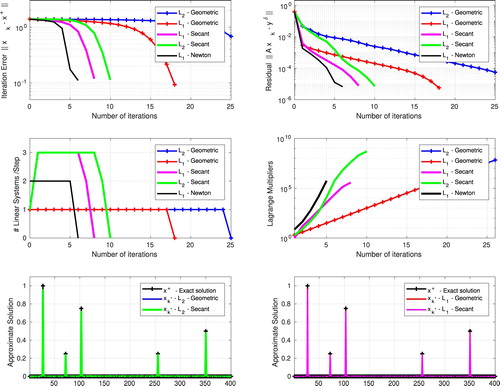
The six pictures in Figure 1 represent:

1. [TOP] Iteration error in $L^2$-norm (left);⁵ residual in $L^2$-norm (right);

2. [CENTER] Number of linear systems/step (left); Lagrange multipliers (right);

3. [BOTTOM] exact solution and reconstructions with $L^2$-penalization (left); exact solution and reconstructions with $L^{1.001}$-penalization (right).

6.2. Image deblurring

In the sequel an application of the nIT method to an image deblurring problem is considered. This is a finite dimensional problem with spaces $X={\mathbb{R}}^n\times {\mathbb{R}}^n$ and $Y={\mathbb{R}}^n\times {\mathbb{R}}^n$. The vector $x\in X$ represents the pixel values of the original image to be restored, and $y\in Y$ contains the pixel values of the observed blurred image. In practice, only noisy blurred data $y^{\delta }\in Y$ satisfying (2(2) $\Vert y^{\delta }-y{\Vert }_Y\le \delta ,$(2) ) is available. The linear transformation A represents some blurring operator.

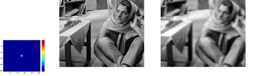
In the numerical simulations we consider the situation where the blur of the image is modelled by a space invariant point spread function (PSF). The exact solution is the $512\times 512$ Barbara image (see Figure 2), and $y^{\delta }$ is obtained adding artificial noise to the exact data y=Ax (here A is the covolution operator corresponding to the PSF).

Figure 2. Image deblurring problem: (LEFT) Point Spread Function; (CENTER) Exact image; (RIGHT) Blurred image.

For this problem the nIT method is implemented with two distinct penalization terms, namely $f(x)=\Vert x{\Vert }_2^2$ ($L^2$ penalization) and $f(x)=\frac{\mu }{2}\Vert x{\Vert }_2^2+TV(x)$ ($L^2+TV$ penalization). Here $\mu >0$ is a regularization parameter and $TV(x)=\Vert \mathrm{\nabla }x{\Vert }_1$ is the total variation norm of x, where $\mathrm{\nabla }:{\mathbb{R}}^n\times {\mathbb{R}}^n\to ({\mathbb{R}}^n\times {\mathbb{R}}^n)\times ({\mathbb{R}}^n\times {\mathbb{R}}^n)$ is the discrete gradient operator. We minimize the Tikhonov functional associated with the $L^2+TV$ penalization term using the ADMM described in Section 5.

In our experiments the values $\mu ={10}^{-4}$, $\delta =0.00001$ and $\tau =1.5$ are used. Moreover, $x_0=y^{\delta }$ and ${\xi }_0={\mathrm{\nabla }}^{\ast }(sign(\mathrm{\nabla }{x}_0))$ are chosen as initial guesses.

In Figure 2, the exact solution, the convolution kernel, and the noisy data are shown. The reconstructed images are shown in Figure 3, while the numerical results are presented in Figure 4. The following methods were implemented:

1. (BLUE) $L^2$-penalization, Geometric sequence;

2. (RED) $L^2+TV$-penalization, Geometric sequence;

3. (PINK) $L^2+TV$-penalization, Secant method;

4. (GREEN) $L^2+TV$-penalization, Adaptive method.

Figure 3. Image deblurring problem: Reconstructions (TOP LEFT) $L^2$–Geometric; (TOP RIGHT) $L^2+TV$–Geometric; (BOTTOM LEFT) $L^2+TV$–Secant; (BOTTOM RIGHT) $L^2+TV$–Adaptive.

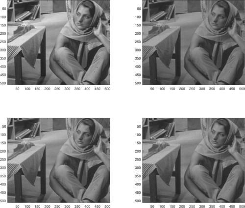
Figure 4. Image deblurring problem: Numerical experiments.

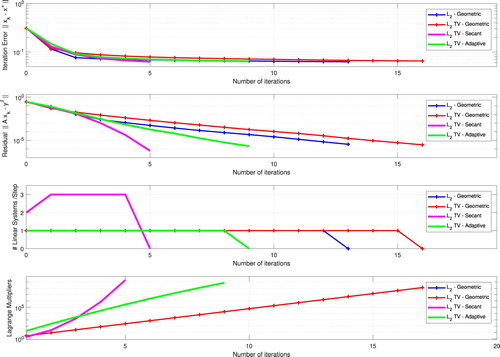
The four pictures in Figure 4 represent:

1. [TOP] Iteration error $\Vert x^{\star }-x_k^{\delta }\Vert$;

2. [CENTER TOP] Residual $\Vert A{x}_k^{\delta }-y^{\delta }\Vert$;

3. [CENTER BOTTOM] Number of linear systems solved in each step;

4. [BOTTOM] Lagrange multiplier ${\lambda }_k$. and $\tau =1.5$. Moreover, the initial guesses $x_0=y^{\delta }$

Remark 6.1

The Tikhonov functional associated with the $L^2+TV$ penalization term is minimized using the ADMM in Section 5. Note that, if $f(x)=\frac{\mu }{2}\Vert x{\Vert }_2^2+\Vert \mathrm{\nabla }x{\Vert }_1$ then one needs to solve $\underset{x\in X}{min}\frac{1}{2}{\lambda }_k\Vert Ax-y^{\delta }{\Vert }^2+\frac{\mu }{2}\Vert x-x_{k-1}^{\delta }{\Vert }^2+\Vert \mathrm{\nabla }x{\Vert }_1-\Vert \mathrm{\nabla }{x}_{k-1}^{\delta }{\Vert }_1-⟨{\xi }_{k-1}^{\delta },x-x_{k-1}^{\delta }⟩$ in each iteration. In order to use ADMM, we sate this problem into the form of (42(42) $\underset{(x,z)\in {\mathbb{R}}^n\times {\mathbb{R}}^m}{min}\{\phi (x)+\varphi (z):Mx+Bz=d\},$(42) ) by defining $z=\mathrm{\nabla }x$, $\phi (x):=\frac{{\lambda }_k}{2}\Vert Ax-y^{\delta }{\Vert }^2+\frac{\mu }{2}\Vert x-x_{k-1}^{\delta }{\Vert }^2-⟨{\xi }_{k-1}^{\delta },x-x_{k-1}^{\delta }⟩$, $\varphi (z)=\Vert z{\Vert }_1-\Vert \mathrm{\nabla }{x}_{k-1}^{\delta }{\Vert }_1$, $M=-\mathrm{\nabla }$, B=I and d=0.

6.3. Inverse potential problem

The third application considered in this section, the Inverse Potentinal Problem (IPP), consists of recovering a coefficient function $x:\mathrm{\Omega }\to \mathcal{R}$, from measurements of the Cauchy data of its corresponding potential on the boundary of the domain $\mathrm{\Omega }=(0,1)\times (0,1)$.

The direct problem is modelled by the linear operator $A:L^2(\mathrm{\Omega })\ni x\mapsto w_{\nu }{|}_{\mathrm{\partial }\mathrm{\Omega }}\in L^2(\mathrm{\partial }\mathrm{\Omega })$, where $w\in H^1(\mathrm{\Omega })$ solves the elliptic boundary value problem (43) $\mathrm{\Delta }w=x,\mathrm{in}\mathrm{\Omega };w=0,\mathrm{at}\mathrm{\partial }\mathrm{\Omega }.$(43) Since $x\in L^2(\mathrm{\Omega })$, the Dirichlet boundary value problem in (43(43) $\mathrm{\Delta }w=x,\mathrm{in}\mathrm{\Omega };w=0,\mathrm{at}\mathrm{\partial }\mathrm{\Omega }.$(43) ) admits a unique solution (known as potential) $w\in H^2(\mathrm{\Omega })\cap H_0^1(\mathrm{\Omega })$ [16].

The inverse problem we are concerned with, consists in determining the piecewise constant source function x from measurements of the Neumann trace of w at $\mathrm{\partial }\mathrm{\Omega }$. Using the above notation, the IPP can be written in the abbreviated form (1(1) $Ax=y,$(1) ), with data $y=w_{\nu }{|}_{\mathrm{\partial }\mathrm{\Omega }}$.

In our implementations we follow [8] in the experimental setup: we set $\mathrm{\Omega }=(0,1)\times (0,1)$ and assume that $x^{\star }\in H^1(\mathrm{\Omega })$ is a function with sharp gradients (see Figure 6).

The boundary value problem (43(43) $\mathrm{\Delta }w=x,\mathrm{in}\mathrm{\Omega };w=0,\mathrm{at}\mathrm{\partial }\mathrm{\Omega }.$(43) ) is solved for w using $x=x^{\star }$, and the exact data $y=w_{\nu }{|}_{\mathrm{\partial }\mathrm{\Omega }}$ for the inverse problem is computed. The noisy data $y^{\delta }$ for the inverse problem is obtained by adding to y a normally distributed noise with zero mean, in order to achieve a prescribed relative noise level.

In our numerical implementations we set $\tau =5$ (discrepancy principle constant), $\delta =0.5\mathrm{\%}$ (relative noise level), and the initial guess $x_0\equiv 1.5$ (a constant function in Ω). For the parameter space we choose $X=L^p(\mathrm{\Omega })$ with p=1.5, while the data space is $Y=L^2(\mathrm{\partial }\mathrm{\Omega })$.

Numerical results for the Inverse potential problem are presented in Figure 5. The following methods are depicted:

1. (RED) $L^p$-penalization, Geometric sequence;

2. (BLACK) $L^p$-penalization, Newton method;

3. (BLUE) $L^p$-penalization, Adaptive method;

Figure 5. Inverse Potential problem: Numerical experiments.

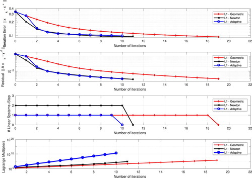
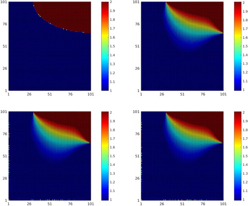
Figure 6. Inverse Potential problem: (TOP LEFT) Exact solution $x^{\star }$. Reconstructions (TOP RIGHT) $L^1$–Geometric; (BOTTOM LEFT) $L^1$–Newton; (BOTTOM RIGHT) $L^1$–Adaptive.

The four pictures in Figure 5 represent: [TOP] Iteration error in $L^p$-norm; [$CENTERTOP$] Residual in $L^2$-norm; [$CENTERBOTTOM$] Number of linear systems/step; [BOTTOM] Lagrange multipliers.

The corresponding reconstruction results are shown in Figure 6: [$TOPLEFT$] Exact Solution; [$TOPRIGHT$] geometric method; [$BOTTOMLEFT$] Newton method; [$BOTTOMLEFT$] Adaptive method.

7. Conclusions

In this manuscript we investigate a novel strategy for choosing the regularization parameters in the nonstationary iterated Tikhonov (nIT) method for solving ill-posed operator equations modelled by linear operators acting between Banach spaces. The novelty of our approach consists in defining strategies for choosing a sequence of regularization parameters (i.e. Lagrange multipliers) for the nIT method.

A preliminary (numerical) investigation of this method was conducted in [9]. In the present manuscript we derive a complete convergence analysis, proving convergence, stability and semi-convergence results (see Section 4). In Sections 6.1 and 6.2 we revisit two numerical applications discussed in [9]. Moreover, in Section 6.3 we investigate a classical benchmark problem in the inverse problems literature, namely the 2D elliptic Inverse Potential Problem.

The Lagrange multipliers are chosen (a posteriori) in order to enforce a fast decay of the residual functional (see Algorithm 1 and Section 4). The computation of these multipliers is performed by means of three distinct methods: (1) a secant type method; (2) a Newton type method; (3) an adaptive method using a geometric sequence with non-constant growth rate, where the rate is updated after each step.

The computation of the iterative step of the nIT method requires the minimization of a Tikhonov Functional (see Section 4). This task is solved here using two distinct methods: (1) in the case of smooth penalization and Banach parameter-spaces the optimality condition (related to the Tikhonov functional) leads to a nonlinear equation, which is solved using a Newton type method; (2) in the case of nonsmooth penalization and Hilbert parameter-space, the ADMM method is used for minimizing the Tikhonov functional.

Disclosure statement

No potential conflict of interest was reported by the authors.

Additional information

Funding

A.L. acknowledges support from CNPq [grant number 311087/2017-5], and from the AvH Foundation.

Notes

1 The differentiability and convexity properties of this functional are independent of the particular choice of $p>1.$

2 This Lemma guarantees that, given a reflexive Banach space E, and a nonempty closed convex set $A\subset E$, then any convex l.s.c proper function $\varphi :A\to (-\mathrm{\infty },\mathrm{\infty }]$ achieves its minimum on A.

3 Here (1(1) $Ax=y,$(1) ) is replaced by $Ag=y^{\delta }$.

4 Notice that we are dealing with a discrete inverse problem, and discretization errors associated to the continuous model are not being considered.

5 For the purpose of comparison, the iteration error is ploted in the in $L^2$-norm for both choices of the parameter space $X=L^2$ and $X=L^{1.001}$.

Appendix

In this appendix we discuss how to compute the Gâteaux derivative of $J_p$. Given $g\in L^p(\mathrm{\Omega })$, the key idea for deriving a formula for $J_p^{\mathrm{\prime }}(g)$ is to observe the differentiability of the function $\gamma :\mathbb{R}\ni x\mapsto p^{-1}|x{|}^p\in \mathbb{R}$. This function is differentiable in $\mathbb{R}$ whenever p>1 and, in this case it holds (A1) ${\gamma }^{\mathrm{\prime }}(x)=|x{|}^{p-1}\mathrm{sign}(x),\mathrm{where}\mathrm{sign}(x)=\{\begin{array}{ll}1,& \mathrm{if}x>0\\ 0,& \mathrm{if}x=0\\ -1,& \mathrm{if}x<0\end{array}.$(A1) Furthermore, γ is twice differentiable in $\mathbb{R}$ if $p\ge 2$, with derivative given by (A2) ${\gamma }^{\mathrm{\prime }\mathrm{\prime }}(x)=(p-1)|x{|}^{p-2}.$(A2) This formula still holds true for $1<p<2,$ but only in $\mathbb{R}\mathrm{\setminus }\{0\}$. In this case, ${\gamma }^{\mathrm{\prime }\mathrm{\prime }}(0)$ does not exist and ${\gamma }^{\mathrm{\prime }\mathrm{\prime }}(x)$ grows to infinity as x approaches to zero.

Since $J_p(g)=(\frac{1}{p}\Vert g{\Vert }_{L^p}^p{)}^{\mathrm{\prime }}$ can be identified with (A3) $J_p\left(g\right)={\left|g\right|}^{p-1}\mathrm{sign}(g)$(A3) (see [10]), which looks very similar to ${\gamma }^{\mathrm{\prime }}$ in (A1(A1) ${\gamma }^{\mathrm{\prime }}(x)=|x{|}^{p-1}\mathrm{sign}(x),\mathrm{where}\mathrm{sign}(x)=\{\begin{array}{ll}1,& \mathrm{if}x>0\\ 0,& \mathrm{if}x=0\\ -1,& \mathrm{if}x<0\end{array}.$(A1) ), the bounded linear operator $J_p^{\mathrm{\prime }}(g):L^p(\mathrm{\Omega })\to L^{p^{\ast }}(\mathrm{\Omega })$ should be in some sense similar to ${\gamma }^{\mathrm{\prime }\mathrm{\prime }}$ in (A2(A2) ${\gamma }^{\mathrm{\prime }\mathrm{\prime }}(x)=(p-1)|x{|}^{p-2}.$(A2) ). We then fix $g\in L^p(\mathrm{\Omega })$ with $p\ge 2$ and try to prove (41(41) $(J_p^{\mathrm{\prime }}(g))(h)=⟨(p-1)|g{|}^{p-2},h⟩,\mathrm{\forall }h\in L^p(\mathrm{\Omega }),$(41) ), i.e. $(J_p^{\mathrm{\prime }}(g))(h)=⟨(p-1)|g{|}^{p-2},h⟩,\mathrm{\forall }h\in L^p(\mathrm{\Omega }),$ where the linear operator $(p-1)|g{|}^{p-2}:h\mapsto (p-1)|g(\cdot ){|}^{p-2}h(\cdot )$ is to be understood in pointwise sense. This ensures that $J_p$ is Gâteaux-differentiable in $L^p(\mathrm{\Omega })$ and its derivative $J_p^{\mathrm{\prime }}$ can be identified with $(p-1)|\cdot {|}^{p-2}$.

Note that, given $h\in L^p(\mathrm{\Omega })$, equality (41(41) $(J_p^{\mathrm{\prime }}(g))(h)=⟨(p-1)|g{|}^{p-2},h⟩,\mathrm{\forall }h\in L^p(\mathrm{\Omega }),$(41) ) holds iff $\underset{t\to 0}{lim}{f}_t=(p-1)|g(\cdot ){|}^{p-2}h(\cdot )$, where $f_t:\mathrm{\Omega }\to \mathbb{R}$ is defined by $f_t(x):=t^{-1}[J_p(g+th)-J_p(g)](x)$. This is equivalent to prove that $\underset{t\to 0}{lim}\Vert f_t-(p-1)|g(\cdot ){|}^{p-2}h(\cdot ){\Vert }_{L^{p^{\ast }}(\mathrm{\Omega })}^{p^{\ast }}=0.$ In view of (A3(A3) $J_p\left(g\right)={\left|g\right|}^{p-1}\mathrm{sign}(g)$(A3) ) and (A2(A2) ${\gamma }^{\mathrm{\prime }\mathrm{\prime }}(x)=(p-1)|x{|}^{p-2}.$(A2) ), it follows that for each $x\in \mathrm{\Omega }$ fixed we have $\begin{array}{rl}\underset{t\to 0}{lim}{f}_t(x)& =\underset{t\to 0}{lim}{t}^{-1}[|g(x)+th(x){|}^{p-1}\mathrm{sign}(g(x)+th(x))-|g(x){|}^{p-1}\mathrm{sign}(g(x))]\\ & =\frac{\mathrm{d}}{\mathrm{d}t}[|g(x)+th(x){|}^{p-1}\mathrm{sign}(g(x)+th(x)){]}_{t=0}\\ & =[(p-1)|g(x)+th(x){|}^{p-2}h(x){]}_{t=0}=(p-1)|g(x){|}^{p-2}h(x).\end{array}$ Thus, making use of Lebesgue's Dominated Convergence Theorem, we conclude that $\begin{array}{rl}\underset{t\to 0}{lim}\Vert f_t-(p-1)|g(\cdot ){|}^{p-2}h(\cdot ){\Vert }_{L^{p^{\ast }}(\mathrm{\Omega })}^{p^{\ast }}& =\underset{t\to 0}{lim}{\int }_{\mathrm{\Omega }}|f_t(x)-(p-1)|g(x){|}^{p-2}h(x){|}^{p^{\ast }}dx\\ & ={\int }_{\mathrm{\Omega }}|\underset{t\to 0}{lim}{f}_t(x)-(p-1)|g(x){|}^{p-2}h(x){|}^{p^{\ast }}\mathrm{d}x=0.\end{array}$ which proves (41(41) $(J_p^{\mathrm{\prime }}(g))(h)=⟨(p-1)|g{|}^{p-2},h⟩,\mathrm{\forall }h\in L^p(\mathrm{\Omega }),$(41) ).

References

- Engl HW, Hanke M, Neubauer A. Regularization of inverse problems. Dordrecht: Kluwer Academic Publishers Group; 1996. (Mathematics and its applications; 375). MR 1408680.
- Hanke M, Groetsch CW. Nonstationary iterated Tikhonov regularization. J Optim Theory Appl. 1998;98(1):37–53. doi: 10.1023/A:1022680629327
- Jin Q, Stals L. Nonstationary iterated Tikhonov regularization for ill-posed problems in Banach spaces. Inverse Probl. 2012;28(3):104011.
- Schuster T, Kaltenbacher B, Hofmann B, et al. Regularization methods in Banach spaces. Berlin: de Gruyter; 2012.
- De Cezaro A, Baumeister J, Leitão A. Modified iterated Tikhonov methods for solving systems of nonlinear ill-posed equations. Inverse Probl Imaging. 2011;5(1):1–17. doi: 10.3934/ipi.2011.5.1
- Jin Q, Zhong M. Nonstationary iterated Tikhonov regularization in Banach spaces with uniformly convex penalty terms. Numer Math. 2014;127(3):485–513. MR 3216817 doi: 10.1007/s00211-013-0594-9
- Lorenz D, Schoepfer F, Wenger S. The linearized bregman method via split feasibility problems: analysis and generalizations. SIAM J Imaging Sci. 2014;7(2):1237–1262. doi: 10.1137/130936269
- Boiger R, Leitão A, Svaiter BF. Range-relaxed criteria for choosing the Lagrange multipliers in nonstationary iterated Tikhonov method. IMA J Numer Anal. 2019;39(1). DOI:10.1093/imanum/dry066
- Machado MP, Margotti F, Leitão A. On nonstationary iterated Tikhonov methods for ill-posed equations in Banach spaces. In: Hofmann B, Leitão A, Zubelli JP, editors. New trends in parameter identification for mathematical models. Cham: Springer International Publishing; 2018. p. 175–193.
- Cioranescu I. Geometry of Banach spaces, duality mappings and nonlinear problems. Dordrecht: Kluwer Academic Publishers Group; 1990. (Mathematics and its applications; 62). MR 1079061.
- Brezis H. Functional analysis, Sobolev spaces and partial differential equations. New York: Springer; 2011. (Universitext). MR 2759829.
- Rockafellar RT Conjugate duality and optimization, Society for Industrial and Applied Mathematics, Philadelphia, PA, 1974, Lectures given at the Johns Hopkins University, Baltimore, Md., June, 1973, Conference Board of the Mathematical Sciences Regional Conference Series in Applied Mathematics, No. 16. MR 0373611.
- Eckstein J, Bertsekas DP. On the Douglas-Rachford splitting method and the proximal point algorithm for maximal monotone operators. Math Program. 1992;55(3):293–318. MR 1168183. doi: 10.1007/BF01581204
- Glowinski R, Marrocco A. Sur l'approximation, par éléments finis d'ordre un, et la résolution, par pénalisation-dualité, d'une classe de problèmes de Dirichlet non linéaires. Rev. Française Automat. Informat. Recherche Opérationnelle Sér. Rouge Anal. Numér.. 1975;9(R-2):41–76. MR 0388811.
- Gabay D, Mercier B. A dual algorithm for the solution of nonlinear variational problems via finite element approximation. Comput Math Appl. 1976;2(1):17–40. doi: 10.1016/0898-1221(76)90003-1
- Evans LC. Partial differential equations. Providence, RI: American Mathematical Society; 1998. (Graduate studies in mathematics; 19).