Source strength identification problem for the three-dimensional inverse heat conduction equations

ABSTRACT

In this paper, we consider the source strength identification problem for the three-dimensional inverse heat conduction equations. The problem is to determine an unknown heat source strength from the measurement data for a specified location. In this process, the direct problem is solved by applying the Green’s function method. Then, this problem can be converted into a Volterra integral equation of the first kind. Further, the Tikhonov and truncated singular value decomposition regularization methods are developed to identify the unknown source strength based on the discrepancy principle for choosing the regularization parameter. Finally, numerical examples are presented to show the feasibility and efficiency of the proposed method.

KEYWORDS:

• Inverse heat conduction problem
• source strength
• integral equation
• regularization

SUBJECT CLASSIFICATIONS CODE:

• 35K05
• 35R30
• 45Q05

1. Introduction

The source strength identification problem, or the inverse heat conduction problem (IHCP) is typically stated as the problem of using the internal temperature to determine the unknown heat source strength function, which has many applications in various branches of engineering and science [1,2]. As is known, the source strength identification problem is severely ill-posed in the sense of Hadamard [3]. In fact, for physical measurements contaminated with small noise, the corresponding solutions have large errors. It is difficult to obtain the numerical solution of this problem. Hence, the regularization method has been used to solve the IHCP. In [4], the Tikhonov regularization method is used to stabilize the solution of the IHCP. In recent years, the regularization method has been proposed for obtaining an efficient solution of the source strength identification problem, see [5–8]. Theoretical investigation of the uniqueness and conditional stability results of the source identification problems are provided in [1,9,10]. The two-dimensional source strength identification problem was developed to solve a Volterra integral equation by utilizing the sequential algorithm [11]. The unknown source strength of a plane surface is identified by using a combination of the regularization and modified conjugate gradient methods [12,13]. The heat conduction equation has been solved by using Green’s function method, and the temperature distribution has been obtained in the series form in terms of circular functions [14,15]. Based on the Green’s function, fundamental solutions have been developed for solving the source strength identification problem [2,3].

This paper is organized as follows. In Section 2, we formulate the three-dimensional inverse heat source strength identification problem. In Section 3, we show that this problem can be converted into a Volterra integral equation of the first kind. The numerical algorithms are derived, and they are given using the Tikhonov regularization and truncated singular value decomposition (TSVD) with the discrepancy principle (DP) to choose the regularization parameter. In Section 4, numerical examples are presented to demonstrate the feasibility and efficiency of the proposed method. Finally, we summarize this paper in Section 5.

2. Description of the problem

The direct heat conduction problem (DHCP) is the determination of the interior temperature with boundary conditions and an initial condition. The mathematical formulation of this problem is given by the three-dimensional heat conduction equations: (1a) $\begin{array}{rl}\frac{\mathrm{\partial }u}{\mathrm{\partial }t}& =a^2\left(\frac{{\mathrm{\partial }}^{2}u}{\mathrm{\partial }{x}^2}+\frac{{\mathrm{\partial }}^{2}u}{\mathrm{\partial }{y}^2}+\frac{{\mathrm{\partial }}^{2}u}{\mathrm{\partial }{z}^2}\right)+g\left(t\right)\delta (x-x_0,y-y_0,z-z_0),\\ & (x,y,z)\in \mathrm{\Omega },t>0,\end{array}$(1a) (1b) $\begin{array}{rl}u(x,y,z,0)& =f(x,y,z),(x,y,z)\in \mathrm{\Omega },\end{array}$(1b) (1c) $\begin{array}{rl}u(0,y,z,t)& =u(L,y,z,t)=0,0\le y\le H,0\le z\le P,t>0,\end{array}$(1c) (1d) $\begin{array}{rl}u(x,0,z,t)& =u(x,H,z,t)=0,0\le x\le L,0\le z\le P,t>0,\end{array}$(1d) (1e) $\begin{array}{rl}u(x,y,0,t)& =u(x,y,P,t)=0,0\le x\le L,0\le y\le H,t>0,\end{array}$(1e) where $\mathrm{\Omega }=\left\{(x,y,z)|0<x<L,0<y<H,0<z<P\right\}$, $\delta (\cdot )$is the Dirac delta function, $(x_0,y_0,z_0)\in \mathrm{\Omega }$, $g\left(t\right)$ is the point heat source strength function, and $a$ denotes the dispersion coefficient.

For the direct problem where the initial condition $f(x,y,z)$ and the heat source strength $g\left(t\right)$ are known, the problem given by (1) is concerned with the determination of the temperature distribution $u(x,y,z,t)$ in the interior region of the solids as a function of the time and position.

For the inverse problem considered here, the initial condition $f(x,y,z)$ is known, and the heat source strength $g\left(t\right)$ is regarded as being unknown. To identify the source strength $g\left(t\right)$, additional information is given by the following measured data: (2) $u(x^{\ast },y^{\ast },z^{\ast },t)=\phi \left(t\right),t>0,$(2) where $(x^{\ast },y^{\ast },z^{\ast })\in \mathrm{\Omega }$. Therefore, the inverse problem can be stated as follows: identify the unknown source strength function $g\left(t\right)$ by utilizing the above-mentioned measured data.

3. Algorithm analysis

3.1. Solution of the direct problem

It is well known that the direct problem (1) can be solved by the Green’s function method [15]. To determine the Green’s function, we consider the homogeneous version of this problem: (3a) $\begin{array}{rl}\frac{\mathrm{\partial }\phi }{\mathrm{\partial }t}& =a^2\left(\frac{{\mathrm{\partial }}^2\phi }{\mathrm{\partial }{x}^2}+\frac{{\mathrm{\partial }}^2\phi }{\mathrm{\partial }{y}^2}+\frac{{\mathrm{\partial }}^2\phi }{\mathrm{\partial }{z}^2}\right),(x,y,z)\in \mathrm{\Omega },t>0,\end{array}$(3a) (3b) $\begin{array}{rl}\phi (x,y,z,0)& =f(x,y,z),(x,y,z)\in \mathrm{\Omega },\end{array}$(3b) (3c) $\begin{array}{rl}\phi (0,y,z,t)& =\phi (L,y,z,t)=0,0\le y\le H,0\le z\le P,t>0,\end{array}$(3c) (3d) $\begin{array}{rl}\phi (x,0,z,t)& =\phi (x,H,z,t)=0,0\le x\le L,0\le z\le P,t>0,\end{array}$(3d) (3e) $\begin{array}{rl}\phi (x,y,0,t)& =\phi (x,y,P,t)=0,0\le x\le L,0\le y\le H,t>0.\end{array}$(3e)

The solution of problem (3) is obtained by the separation of variables: (4) $\begin{array}{rl}\phi (x,y,z,t)& ={\int }_0^L{\int }_0^H{\int }_0^P\{\frac{8}{LHP}\sum _{m=1}^{\mathrm{\infty }}\sum _{n=1}^{\mathrm{\infty }}\sum _{p=1}^{\mathrm{\infty }}\sin \left(\frac{m\pi x}{L}\right)\sin \left(\frac{n\pi y}{H}\right)\sin \left(\frac{p\pi z}{P}\right)\\ & \times \sin \left(\frac{m\pi x^{\mathrm{\prime }}}{L}\right)\sin \left(\frac{n\pi y^{\mathrm{\prime }}}{H}\right)\sin \left(\frac{p\pi z^{\mathrm{\prime }}}{P}\right)\\ & \times e^{-a^2[{\left(\frac{m\pi }{L}\right)}^2+{\left(\frac{n\pi }{H}\right)}^2+{\left(\frac{p\pi }{P}\right)}^2]t}\}f(x^{\mathrm{\prime }},y^{\mathrm{\prime }},z^{\mathrm{\prime }})\text{d}{x}^{\mathrm{\prime }}\text{d}{y}^{\mathrm{\prime }}\text{d}{z}^{\mathrm{\prime }}.\end{array}$(4) Thus, the Green’s function is obtained as (5) $\begin{array}{rl}G(x,y,z,x^{\mathrm{\prime }},y^{\mathrm{\prime }},z^{\mathrm{\prime }},t)& =\frac{8}{LHP}\sum _{m=1}^{\mathrm{\infty }}\sum _{n=1}^{\mathrm{\infty }}\sum _{p=1}^{\mathrm{\infty }}\sin (\frac{m\pi x}{L})\sin (\frac{n\pi y}{H})\sin (\frac{p\pi z}{P})\sin (\frac{m\pi x^{\mathrm{\prime }}}{L})\\ & \times \sin (\frac{n\pi y^{\mathrm{\prime }}}{H})\sin (\frac{p\pi z^{\mathrm{\prime }}}{P})\\ & \times e^{-a^2[{\left(\frac{m\pi }{L}\right)}^2+{\left(\frac{n\pi }{H}\right)}^2+{\left(\frac{p\pi }{P}\right)}^2]t}.\end{array}$(5) The solution of problem (3) in terms of the Green’s function is given as (6) $\phi (x,y,z,t)={\int }_0^L{\int }_0^H{\int }_0^{P}f(x^{\mathrm{\prime }},y^{\mathrm{\prime }},z^{\mathrm{\prime }})G(x,y,z,x^{\mathrm{\prime }},y^{\mathrm{\prime }},z^{\mathrm{\prime }},t)\text{d}{x}^{\mathrm{\prime }}\text{d}{y}^{\mathrm{\prime }}\text{d}{z}^{\mathrm{\prime }}.$(6) Because the direct problem is nonhomogeneous, the desired Green’s function is obtained by substituting $t$ with $(t-\tau )$ in (5), and it has the following form: (7) $\begin{array}{rl}G(x,y,z,x^{\mathrm{\prime }},y^{\mathrm{\prime }},z^{\mathrm{\prime }},t-\tau )& =\frac{8}{LHP}\sum _{m=1}^{\mathrm{\infty }}\sum _{n=1}^{\mathrm{\infty }}\sum _{p=1}^{\mathrm{\infty }}\sin (\frac{m\pi x}{L})\sin (\frac{n\pi y}{H})\sin (\frac{p\pi z}{P})\\ & \times \sin (\frac{m\pi x^{\mathrm{\prime }}}{L})\sin (\frac{n\pi y^{\mathrm{\prime }}}{H})\sin (\frac{p\pi z^{\mathrm{\prime }}}{P})\\ & \times e^{-a^2[{\left(\frac{m\pi }{L}\right)}^2+{\left(\frac{n\pi }{H}\right)}^2+{\left(\frac{p\pi }{P}\right)}^2](t-\tau )}.\end{array}$(7) Then, the solution of the direct problem can be given as (8) $\begin{array}{rl}u(x,y,z,t)& ={\int }_0^L{\int }_0^H{\int }_0^{P}f(x^{\mathrm{\prime }},y^{\mathrm{\prime }},z^{\mathrm{\prime }})G(x,y,z,x^{\mathrm{\prime }},y^{\mathrm{\prime }},z^{\mathrm{\prime }},t)\text{d}{x}^{\mathrm{\prime }}\text{d}{y}^{\mathrm{\prime }}\text{d}{z}^{\mathrm{\prime }}\\ & +{\int }_0^t{\int }_0^L{\int }_0^H{\int }_0^{P}G(x,y,z,x^{\mathrm{\prime }},y^{\mathrm{\prime }},z^{\mathrm{\prime }},t-\tau \left)g\right(\tau \left)\delta \right(x^{\mathrm{\prime }}-x_0,y^{\mathrm{\prime }}-y_0,z^{\mathrm{\prime }}-z_0)\\ & \times \text{d}{x}^{\mathrm{\prime }}\text{d}{y}^{\mathrm{\prime }}\text{d}{z}^{\mathrm{\prime }}\text{d}\tau ,\end{array}$(8) and it can be simplified as follows: (9) $\begin{array}{rl}u(x,y,z,t)& ={\int }_0^L{\int }_0^H{\int }_0^{P}f(x^{\mathrm{\prime }},y^{\mathrm{\prime }},z^{\mathrm{\prime }})G(x,y,z,x^{\mathrm{\prime }},y^{\mathrm{\prime }},z^{\mathrm{\prime }},t)\text{d}{x}^{\mathrm{\prime }}\text{d}{y}^{\mathrm{\prime }}\text{d}{z}^{\mathrm{\prime }}\\ & +{\int }_0^{t}g\left(\tau \right)G(x,y,z,x_0,y_0,z_0,t-\tau )\text{d}\tau .\end{array}$(9)

3.2. Discretization of the heat source strength identification problem

From (9), we have (10) $\begin{array}{rl}u(x,y,z,t)-& {\int }_0^L{\int }_0^H{\int }_0^{P}f(x^{\mathrm{\prime }},y^{\mathrm{\prime }},z^{\mathrm{\prime }})G(x,y,z,x^{\mathrm{\prime }},y^{\mathrm{\prime }},z^{\mathrm{\prime }},t)\text{d}{x}^{\mathrm{\prime }}\text{d}{y}^{\mathrm{\prime }}\text{d}{z}^{\mathrm{\prime }}\\ & ={\int }_0^{t}g\left(\tau \right)G(x,y,z,x_0,y_0,z_0,t-\tau )\text{d}\tau .\end{array}$(10) According to (2), the source strength identification problem is reduced to solve the Volterra integral equation of the first kind, which is stated as follows: (11) $w\left(t\right)={\int }_0^{t}g\left(\tau \right)G(x^{\ast },y^{\ast },z^{\ast },x_0,y_0,z_0,t-\tau )\text{d}\tau ,$(11) where (12) $\begin{array}{rl}w\left(t\right)& =u(x^{\ast },y^{\ast },z^{\ast },t)-{\int }_0^L{\int }_0^H{\int }_0^{P}f(x^{\mathrm{\prime }},y^{\mathrm{\prime }},z^{\mathrm{\prime }})G(x^{\ast },y^{\ast },z^{\ast },x^{\mathrm{\prime }},y^{\mathrm{\prime }},z^{\mathrm{\prime }},t)\text{d}{x}^{\mathrm{\prime }}\text{d}{y}^{\mathrm{\prime }}\text{d}{z}^{\mathrm{\prime }}\\ & =\phi \left(t\right)-{\int }_0^L{\int }_0^H{\int }_0^{P}f(x^{\mathrm{\prime }},y^{\mathrm{\prime }},z^{\mathrm{\prime }})G(x^{\ast },y^{\ast },z^{\ast },x^{\mathrm{\prime }},y^{\mathrm{\prime }},z^{\mathrm{\prime }},t)\text{d}{x}^{\mathrm{\prime }}\text{d}{y}^{\mathrm{\prime }}\text{d}{z}^{\mathrm{\prime }}.\end{array}$(12)

Since $w\left(t\right)$ contains a triple-integral, which makes it difficult to obtain the exact value, we approximate it by using the Gauss–Legendre quadrature. To identify the source strength $g\left(t\right)$ in (11), we employ a numerical method which is obtained by using a mid-rectangle quadrature.

The interval $[0,t]$ can be subdivided into intervals of width $h=t/N$, $t_i=ih$, $i=1,2,\cdots ,N$. We have (13) $\begin{array}{rl}w\left(t_i\right)& ={\int }_0^{t_i}g\left(\tau \right)G(x^{\ast },y^{\ast },z^{\ast },x_0,y_0,z_0,t_i-\tau )\text{d}\tau \\ & ={\int }_0^{t_1}g\left(\tau \right)G(x^{\ast },y^{\ast },z^{\ast },x_0,y_0,z_0,t_i-\tau )\text{d}\tau \\ & +{\int }_{t_1}^{t_2}g\left(\tau \right)G(x^{\ast },y^{\ast },z^{\ast },x_0,y_0,z_0,t_i-\tau )\text{d}\tau +\cdots \\ & +{\int }_{t_{{}_{i-1}}}^{t_i}g\left(\tau \right)G(x^{\ast },y^{\ast },z^{\ast },x_0,y_0,z_0,t_i-\tau )\text{d}\tau .\end{array}$(13) If the mid-rectangle rule is used to approximate each integral, then (14) $\begin{array}{rl}w\left(t_i\right)\approx & h\left[G\right(x^{\ast },y^{\ast },z^{\ast },x_0,y_0,z_0,t_i-\frac{h}{2}\left)g\right(\frac{h}{2})+G(x^{\ast },y^{\ast },z^{\ast },x_0,y_0,z_0,t_i-\frac{3h}{2}\left)g\right(\frac{3h}{2})+\cdots \\ & +G(x^{\ast },y^{\ast },z^{\ast },x_0,y_0,z_0,t_i-\frac{2i-1}{2}h)g\left(\frac{2i-1}{2}h\right)].\end{array}$(14) For convenience, we denote $G(x^{\ast },y^{\ast },z^{\ast },x_0,y_0,z_0,t_i-((2j-1)/2\left)h\right)$ as $G_{ij}$, $g\left(\right((2j-1)/2\left)h\right)$ as $g_j$, and $w\left(t_i\right)$ as $w_i$. The equation can be written as follows: (15) $w_i\approx h[G_{i1}{g}_1+G_{i2}{g}_2+\cdots +G_{ij}{g}_j],$(15) where $i,j=1,2,\cdots ,N;i\ge j$. This can also be written in the matrix form: (16) $Gg=w,$(16) where $G$ is the matrix of the coefficients: (17) $G=h\left[\begin{array}{ccccc}{G}_{11}& 0& 0& \cdots & 0\\ G_{21}& G_{22}& 0& \cdots & 0\\ ⋮& ⋮& ⋮& \ddots & ⋮\\ G_{(N-1)1}& G_{(N-1)2}& G_{(N-1)3}& \cdots & 0\\ G_{N1}& G_{N2}& G_{N(N-1)}& \cdots & G_{NN}\end{array}\right],$(17) $g$ is the vector of solutions: (18) $g=(g_1,g_2,\cdots ,g_N{)}^T,$(18) and $w$ is the vector of the nonhomogeneous part: (19) $w=(w_1,w_2,\cdots ,w_N{)}^T.$(19)

3.3. Regularization algorithms for the identification of heat source strength

In general, the Volterra integral equation of the first kind is ill-posed. In the finite-dimensional case, the condition number of matrix $G$ is very large. Hence, the problem (16) is ill-conditioned. Generally, the regularization method is considered to be an effective tool for solving an ill-conditioned problem. Therefore, we apply the Tikhonov regularization and TSVD to find a stable approximate solution to (16).

To achieve that, the Tikhonov regularization is proposed to solve the following: (20) $g_{\alpha }=\arg \underset{g\in R^N}{min}{J}_{\alpha }\left(g\right)=(||Gg-w|{|}_2^2+\alpha ||g|{|}_2^2),$(20) where $\alpha (\alpha >0)$ is the regularization parameter. The computation of the approximate solution $g_{\alpha }$ consists of solving the augmented normal equation (21) $(G^{T}G+\alpha I)g_{\alpha }=G^{T}w,$(21) where $G^T$ is the adjoint operator of $G$, and $I$ is the identity operator.

The singular value decomposition (SVD) of the matrix $G$ is given by (22) $G=\sum _{j=1}^N{u}_j{\sigma }_j{v}_j^T,$(22) where the left and right singular vectors $u_j$ and $v_j$ are orthonormal, and the singular values ${\sigma }_j$ are nonnegative and nonincreasing, ${\sigma }_1\ge {\sigma }_2\ge \cdots \ge {\sigma }_N\ge 0$. Then, the Tikhonov regularization solution of (16) obtained using SVD can be expressed as follows: (23) $g_{\alpha }=\sum _{j=1}^N\frac{{\sigma }_j^{}}{{\sigma }_j^2+\alpha }{u}_j^{T}w{v}_j.$(23)

As another approach to find a stable approximate solution to (16), we determine an approximate solution of the least-squares problems of the form (24) $\underset{g\in R^N}{min}||Gg-w|{|}_2^{},$(24) and the least-squares solution can be expressed as (25) $g_{LS}=G^{+}w=\sum _{j=1}^r\frac{u_j^{T}w}{{\sigma }_j}{v}_j,$(25) where $G^{+}$ denotes the pseudo-inverse of $G$. Owing to the singular values of $G$ ordered according to (26) ${\sigma }_1\ge {\sigma }_2\ge \cdots \ge {\sigma }_r>{\sigma }_{r+1}=\cdots {\sigma }_N=0,$(26) the singular value gradually tends to zero, and the least-squares solution is far from the exact solution. The TSVD screens outs the smallest singular values of $G$, those that are less than an imposed threshold. In this case, the threshold is set at ${\sigma }_k$ when $k\le r$. We obtain the TSVD regularization solution as (27) $g_k=\sum _{j=1}^k\frac{u_j^{T}w}{{\sigma }_j}{v}_j,$(27) where $k$ is the regularization parameter.

In practical applications, the data are often affected by the Gaussian random noise. Hence, we consider the determination of the regularization parameters using the following model: (28) $w=Gg+\epsilon ,$(28) where $\epsilon$ is an i.i.d. Gaussian random vector with variance ${\sigma }^2$, and we denote $\epsilon \sim N(0,{\sigma }^{2}I)$.

To obtain an effective approximate solution to the original ill-posed problem, determining the regularization parameter will be very important. Next, we introduce the DP, which is a standard regularization parameter method used for the inverse problem. When the DP is used to determine the regularization parameter, where $\upsilon$ satisfies: (29) $||G{g}_{\upsilon }-w|{|}_2^2=\mathrm{E}\left[||\epsilon |{|}_2^2\right]=N{\sigma }^2,$(29) we define the discrepancy function as (30) $D\left(\upsilon \right)=||G{g}_{\upsilon }-w|{|}_2^2-N{\sigma }^2=0.$(30) From (30), we compute the value of $\upsilon$. The function $D(\cdot )$ is simplified using the SVD, which is given as follows for the Tikhonov regularization and TSVD, respectively, (31) $D\left(\alpha \right)=\sum _{i=1}^N\frac{{\alpha }^2{\left(u_i^{T}w\right)}^2}{{({\sigma }_i^2+\alpha )}^2}-N{\sigma }^2,$(31) (32) $D\left(k\right)=\sum _{i=k+1}^N{\left(u_i^{T}w\right)}^2-N{\sigma }^2.$(32) Therefore, the value $\alpha$ can be obtained using methods such as Newton’s method when using the DP for Tikhonov regularization. Moreover, the value $k$ can choose the first $k$such that $D\left(k\right)\le 0$ when using the DP for TSVD.

4. Numerical examples

For the source strength identification problem (1)–(2), let $\mathrm{\Omega }=\left\{\right(x,y,z)|0<x<1,0<y<1,0<z<1\}$, $0<t\le 1$, $a=1$. We consider the following equations: (33) $\begin{array}{rl}\frac{\mathrm{\partial }u}{\mathrm{\partial }t}& =\frac{{\mathrm{\partial }}^{2}u}{\mathrm{\partial }{x}^2}+\frac{{\mathrm{\partial }}^{2}u}{\mathrm{\partial }{y}^2}+\frac{{\mathrm{\partial }}^{2}u}{\mathrm{\partial }{z}^2}+g\left(t\right)\delta (x-0.5,y-0.5,z-0.5),\end{array}$(33) (34) $\begin{array}{rl}u(x,y,z,0)& =f(x,y,z),\end{array}$(34) (35) $\begin{array}{rl}u(0,y,z,t)& =u(1,y,z,t)=0,\end{array}$(35) (36) $\begin{array}{rl}u(x,0,z,t)& =u(x,1,z,t)=0,\end{array}$(36) (37) $\begin{array}{rl}u(x,y,0,t)& =u(x,y,1,t)=0,\end{array}$(37) (38) $\begin{array}{rl}u(0.25,0.25,0.25,t)& =\phi \left(t\right),\end{array}$(38) where $f(x,y,z)=\sin \left(\pi x\right)\sin \left(\pi y\right)\sin \left(\pi z\right)$.

We can see that $G(x,y,z,x^{\mathrm{\prime }},y^{\mathrm{\prime }},z^{\mathrm{\prime }},t)$ is an infinite series and it cannot be used directly for numerical computations. Therefore, we adopt (39) $\begin{array}{rl}G(x,y,z,x^{\mathrm{\prime }},y^{\mathrm{\prime }},z^{\mathrm{\prime }},t)\approx & \frac{8}{LHP}\sum _{m=1}^{100}\sum _{n=1}^{100}\sum _{p=1}^{100}\sin (\frac{m\pi x}{L})\sin (\frac{n\pi y}{H})\sin (\frac{p\pi z}{P})\\ & \times \sin (\frac{m\pi x^{\mathrm{\prime }}}{L})\sin (\frac{n\pi y^{\mathrm{\prime }}}{H})\sin (\frac{p\pi z^{\mathrm{\prime }}}{P})\\ & \times e^{-a^2[{\left(\frac{m\pi }{L}\right)}^2+{\left(\frac{n\pi }{H}\right)}^2+{\left(\frac{p\pi }{P}\right)}^2]t},\end{array}$(39) which guarantees the convergence of the series.

Firstly, assuming that the source strength is known, let $g\left(t\right)=t{e}^{-8t}$. In the computations, we take $N=40$. The additional values are obtained using the Gauss–Legendre quadrature in discrete time with time step $\mathrm{\Delta }t=0.025$ and at $(0.25,0.25,0.25)$. The obtained values are listed in Table 1. Then, the values will be used to determine $g\left(t\right)$.

Table 1. Additional values of $u(0.25,0.25,0.25,t_i)$.

$t_i$	0.1	0.2	0.3	0.4	0.5
$u(0.25,0.25,0.25,t_i)$	0.01986922	0.00318231	0.00179090	0.00111926	0.00065214
$t_i$	0.6	0.7	0.8	0.9	1.0
$u(0.25,0.25,0.25,t_i)$	0.00036048	0.00019231	0.00010004	0.000051076	0.00002570

We use the $L_{\mathrm{\infty }}$ error norm and the relative error (RE) to measure the difference between the numerical and exact solutions. The $L_{\mathrm{\infty }}$ error norm [16] is defined by (40) $L_{\mathrm{\infty }}=\underset{0\le i\le N}{max}|g\left(t_i\right)-\tilde{g}\left(t_i\right)|,$(40) and the RE [16] is defined by (41) $\text{RE}=\sqrt{\sum _{i=1}^N{\left(g\right(t_i)-\tilde{g}(t_i\left)\right)}^2}/\phantom{\sqrt{\sum _{i=1}^N{\left(g\right(t_i)-\tilde{g}(t_i\left)\right)}^2}\sqrt{\sum _{i=1}^N{\left(g\right(t_i\left)\right)}^2}}\sqrt{\sum _{i=1}^N{\left(g\right(t_i\left)\right)}^2},$(41) where $t_i$, $N$, $g\left(t\right)$, $\tilde{g}\left(t\right)$ denote the test points, the total number of uniformly distributed points on the interval $[0,1]$, the exact solution and the numerical solution, respectively.

Example: First, we consider the source strength identification problem in a non-noise jamming situation. We obtain the reconstructions for the source strength $g\left(t\right)$ with $\sigma =0$.

To solve the source strength identification problem, we apply the Tikhonov regularization and TSVD methods. The Tikhonov regularization parameter $\alpha$ and the TSVD regularization parameter $k$ are chosen using the DP; the $L_{\mathrm{\infty }}$ error norm and the RE are listed in Table 2. From the table, we can see that the TSVD errors are smaller than those of the Tikhonov regularization. Figures 1 and 2 compare the exact solution with its numerical solution that used the regularization method. As shown in the figures, the regularization method to identify the source strength is in good agreement with the exact solution in the non-noise jamming situation.

Figure 1. Comparison of exact and numerical solutions using Tikhonov regularization with $\sigma =0$.

Figure 2. Comparison of exact and numerical solutions using TSVD with $\sigma =0$.

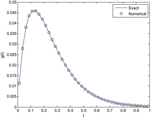
Table 2. $L_{\mathrm{\infty }}$ error norm and RE for $g\left(t\right)$, with $\sigma =0$.

Method	Parameter	RE	$L_{\mathrm{\infty }}$
Tikhonov	6.35906253 × 10^−5	0.02796904	7.62407172 × 10^−4
TSVD	40	6.07527492 × 10^−8	4.19828995 × 10^−9

Next, we consider the source strength identification problem in a Gaussian random noise jamming situation. In our experiment, we considered the Gaussian random noise with mean zero and standard deviation (42) $\sigma =\frac{1}{50}\sqrt{\sum _{i=1}^N{g}_i^2/\phantom{\sum _{i=1}^N{g}_i^{2}N}N},$(42) the noisy data are generated by (28). We take $N=40$, and obtained $\sigma =$2.16583542×10⁻⁵. The Tikhonov regularization and TSVD method are applied to reconstruct the source strength $g\left(t\right)$. In Figures 3 and 4, we compare the numerical solution of the proposed method with the exact solution. From these figures, it can be seen that the numerical solution is in agreement with the exact solution. The regularization parameter, $L_{\mathrm{\infty }}$ error norm and RE are presented in Table 3. As shown in Table 3, the REs are maintained within an acceptable range, and the $L_{\mathrm{\infty }}$ error norm for the Tikhonov regularization is smaller than that for the TSVD.

Figure 3. Comparison of exact and numerical solutions using Tikhonov regularization with $\sigma =$2.16583542×10⁻⁵.

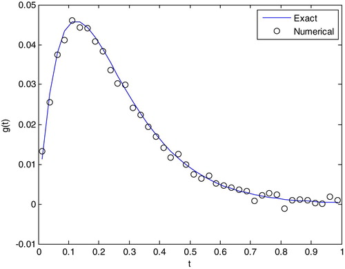
Figure 4. Comparison of exact and numerical solutions using TSVD with $\sigma =$2.16583542×10⁻⁵.

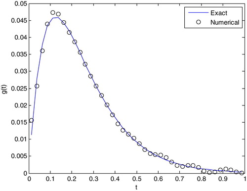
Table 3. $L_{\mathrm{\infty }}$ error norm and RE for $g\left(t\right)$, with $\sigma =$2.16583542×10⁻⁵.

Method	Parameter	RE	$L_{\mathrm{\infty }}$
Tikhonov	6.51184081 × 10^−5	0.05079719	0.00190189
TSVD	15	0.04314080	0.00431313

From the previous numerical example, it can be seen that the TSVD numerical results are quite satisfactory in the non-noise jamming situation. In the noise jamming situation, the reconstruction results for different regularization methods are considered acceptable.

5. Conclusion

In this paper, we presented the Tikhonov regularization and TSVD method to solve the three-dimensional inverse source strength identification problem based on the Green’s function and Volterra integral equation of the first kind. Numerical examples have been provided to check the proposed method for a non-noise jamming situation and a Gaussian random noise jamming situation. The results show that the proposed method is feasible and effective in identifying the unknown source strength.

Acknowledgements

We would like to thank the referees for constructive suggestions and comments.

Disclosure statement

No potential conflict of interest was reported by the authors.

Additional information

Funding

This research was supported by the Natural Science Basic Research Plan in Shaanxi Province of China [grant number 2019JM-284].

References

- Ling L, Takeuchi T. Point sources identification problems for heat equations. Commun Comput Phys. 2009;5:897–913.
- Liang Y, Fu CL, Yang FL. The method of fundamental solutions for the inverse heat source problem. Eng Anal Bound Elem. 2008;32:216–222. doi: 10.1016/j.enganabound.2007.08.002
- Hon YC, Li M, Melnikov YA. Inverse source identification by Green’s function. Eng Anal Bound Elem. 2010;34:352–358. doi: 10.1016/j.enganabound.2009.09.009
- Duda P. Solution of inverse heat conduction problem using the Tikhonov regularization method. J Therm Sci. 2017;26:60–65. doi: 10.1007/s11630-017-0910-2
- Yi Z, Murio DA. Source term identification in 1-D IHCP. Comput Math Appl. 2004;47:1921–1933. doi: 10.1016/j.camwa.2002.11.025
- Qian A, Li Y. Optimal error bound and generalized Tikhonov regularization for identifying an unknown source in the heat equation. J Math Chem. 2011;49:765–775. doi: 10.1007/s10910-010-9774-3
- Liang Y, Yang FL, Fu CL. A new numerical method for the inverse source problem from a Bayesian perspective. Int J Numer Meth Eng. 2015;85(11):1460–1474.
- Cheng W, Zhao LL, Fu CL. Source term identification for an axisymmetric inverse heat conduction problem. Comput Math Appl. 2010;59(1):142–148. doi: 10.1016/j.camwa.2009.08.038
- Cannon JR, Perezesteva S. Uniqueness and stability of 3D heat sources. Inverse Probl. 1999;7:57–62. doi: 10.1088/0266-5611/7/1/006
- Choulli M, Yamamoto M. Conditional stability in determining a heat source. J Inverse Illposed Probl. 2004;12:233–243. doi: 10.1515/1569394042215856
- Shidfar A, Zakeri A, Neisi A. A two-dimensional inverse heat conduction problem for estimating heat source. Int J Math Math Sci. 2005;10:1633–1641. doi: 10.1155/IJMMS.2005.1633
- Huang CH, Ozisik MN. Inverse problem of determining the unknown strength of an internal plane heat source. J Franklin Inst. 1992;329:751–764. doi: 10.1016/0016-0032(92)90086-V
- Huang CH, Li JX, Kim S. An inverse problem in estimating the strength of contaminant source for groundwater systems. Appl Math Model. 2008;32:417–431. doi: 10.1016/j.apm.2006.12.009
- Gaikwad KR, Ghadle KP. Three dimensional non-homogeneous thermoelastic problem in a thick rectangular plate due to internal heat generation. South Afr J Pure Appl Math. 2011;5:26–38.
- Ozisik MN. Heat conduction. 2nd ed. New York: Wiley-Interscience; 1993.
- Min T, Geng B, Ren J. Inverse estimation of the initial condition for the heat equation. Int J Pure Appl Math. 2013;82:581–593. doi: 10.12732/ijpam.v82i4.7