Application of an adaptive MCMC method for the heat flux estimation

ABSTRACT

Based on Bayesian inference, an adaptive single component Metropolis–Hastings (SCMH) sampling algorithm is presented to estimate the surface heat flux which is a typical inverse heat conduction problem. The surface heat flux is expressed by two different basis functions, the piecewise linear function and the Fourier series, and for speeding up convergence process, the parameters of the Fourier series are arbitrarily decoupled in the burn-in period. For validating and analysing the performance of the sampling algorithm, several cases are discussed. The results show that the adaptive SCMH sampling algorithm is feasible and has accuracy comparable to the conjugate gradient method (CGM), and decoupling method can successively shorten the burn-in period. It also can be found that ‘adaptive’ algorithm can obviously accelerate the convergence process. Furthermore, the performances of the two basis functions are also analysed. Because of the correlation, the paths of Markov Chain of the Fourier coefficients seem more ‘random’, which indicated that the algorithm with Fourier series is more efficient than that with piecewise linear function. The influence of the number of parameters is also studied, which is similar as the regularization of the CGM, the fewer the parameters is, the smoother the estimated heat flux becomes.

KEYWORDS:

• Inverse heat conduction problems
• Bayesian inference
• Markov chain Monte Carlo method
• adaptive method
• ill-posed

2010 MSC MATHEMATICS SUBJECT CLASSIFICATIONS:

• 80A20
• 80A23
• 65C05
• 65C40

Nomenclature

Symbol	=	Meaning (SI Unit)
Cp	=	Heat capacity (J/kg K)
k	=	Thermal conductivity (W/m K)
L	=	Length (m)
m	=	Number of measurement time step
n	=	Number of estimating parameters
N	=	Gauss distribution
p	=	Probability density function (PDF)
q	=	The proposal distribution
Q	=	Heat flux (W/m2)
T	=	Temperature (K)
t	=	Time (s)
u	=	Random value from uniform distribution
U	=	Uniform distribution
v	=	Measurement noise (K)
x	=	Parameter of heat flux
y	=	Measured temperature (K)
Y	=	Fourier coefficients of temperature
z	=	Coordinate (m)
ρ	=	Density (kg/m3)
σ	=	Standard deviation (K)
τ	=	Standard deviation of proposal distribution

1. Introduction

The surface heat flux estimated by using the internal temperature of the object is a typical inverse heat conduction problem (IHCP) and an ill-posed problem in mathematics. And it is often solved with inverse methods and optimization methods [1–7], such as the space marching method, the adjoint equation method, the sequential function method and Laplace transform technique. But inverse methods are known to suffer from poor calculation stability, optimization methods easy fall into the local extreme and need a proper regularization technique to deal with the ill-posedness.

Because Bayesian inference can be used to express and solve inverse problems by using the probabilistic language model, it is widely concerned in different research fields [8–10]. The fundamental of Bayesian inference is to treat unknown parameters as random variables described in form of probability function, and the estimation of unknown parameters are obtained by sampling the posterior distribution in the process of solving inverse problems. Compared with traditional methods, Bayesian inference has two advantages. Firstly, the prior information can be easily incorporated into the solving process of Bayesian inference to reduce the uncertainty of the estimation results. Secondly, Bayesian inference can give the globally most probable solution and probability distribution of solution simultaneously [11].

So in the references [12–16], Bayesian inference is also extended to estimate thermal conductivity, thermal resistance, internal heat generation and surface heat flux. But in this work, the performance of sampling algorithm is a major concern. For speeding up algorithm, an adaptive sampling algorithm and a decoupling method for parameters are developed to estimate the surface heat flux. Then the heat flux is reconstructed by two different basis functions, piecewise linear function and Fourier series, and the performances of different basis functions are also compared.

2. Mathematic model

A typical one-dimensional surface heat flux estimation problem is sketched in Figure 1, a finite slab is subjected to a heat flux on the left boundary and insulated on right boundary. The governing equations can be written as: (1) $\rho C_p\frac{\mathrm{\partial }T}{\mathrm{\partial }t}=\frac{\mathrm{\partial }}{\mathrm{\partial }z}\left(k\frac{\mathrm{\partial }T}{\mathrm{\partial }z}\right)$(1)

Figure 1. Sketch of heat flux inversion.

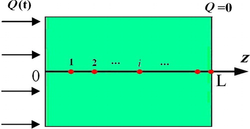
Boundary conditions at z = 0, $-k\left(\mathrm{\partial }T/\mathrm{\partial }z\right)=Q\left(t\right)$; at z = L, $-k\left(\mathrm{\partial }T/\mathrm{\partial }z\right)=0$;

Initial condition at t = 0, T = T₀; (2) $\text{Measurement equation}:y(z_i,t)=\tilde{y}(z_i,t)+v(z_i,t),i=1,n_m$(2) where ρ is the density, C_p is the heat capacity per unit volume, L is the thickness, [0, t_f] is the time span, n_m is the number of measurement points and z_i (i = 1, n_m) are the coordinates of measurement points, y is the temperature measurements, $\tilde{y}$ is the exact temperature and v is the measurement noise. In the heat flux estimation problem, the surface heat flux Q(t) is unknown and need to be rebuilt from temperature measurements shown in Equation (2).

3. Markov chain Monte Carlo method

3.1. Bayesian statistical modelling

The fundamental of Bayesian inference is to treat unknown parameters as random variables and to define a prior distribution p(x). After obtaining data, the corresponding posterior distribution can be derived from the prior distribution p(x) by using the Bayesian function shown as: (3) $p\left(x|y\right)=\frac{p\left(x\right)p\left(y|x\right)}{p\left(y\right)}\propto p\left(x\right)p\left(y|x\right)$(3) where y is the measurements, p(x|y) is the posterior Probability Density Function (PDF), p(y|x) is the conditional PDF, p(y) is the prior distribution.

When the function shown above is used to resolve the heat flux estimation, the measurement y is defined as the temperature measurement which is the sum of the exact temperature and white noise which obey Gaussian distribution with zero mean value and standard deviation σ_y. $\mathbf{\text{x}}$ is defined as the parameters of the heat flux. Then the corresponding conditional PDF for $\mathbf{\text{y}}$ can be written as (4) $p\left(\mathbf{\text{y}}|\mathbf{\text{x}}\right)=\frac{1}{{\left(2\pi {\sigma }_y^2\right)}^{m/2}}\exp \left\{-\frac{{\left(\mathbf{\text{y}}-\widetilde{\mathbf{\text{y}}}\right)}^T\left(\mathbf{\text{y}}-\widetilde{\mathbf{\text{y}}}\right)}{2{{\sigma }_y}^2}\right\}$(4) where m is the number of measurement time steps. Then the posterior distribution of $\mathbf{\text{x}}$ can be derived from the conditional PDF and prior distribution. (5) $p\left(\mathbf{\text{x}}|\mathbf{\text{y}}\right)\propto \prod _{i=1}^{n}p\left(x_i\right)\cdot \frac{1}{{\left(2\pi {\sigma }_y^2\right)}^{m/2}}\exp \left\{-\frac{{\left(\mathbf{\text{y}}-\widetilde{\mathbf{\text{y}}}\right)}^T\left(\mathbf{\text{y}}-\widetilde{\mathbf{\text{y}}}\right)}{2{{\sigma }_y}^2}\right\}$(5) where n is the number of estimating parameters.

In practical computation, when the parameter $\mathbf{\text{x}}$ is specified, the exact temperature $\widetilde{\mathbf{\text{y}}}$ can be solved with finite control volume (FCV) method, which is verified with analytical solution in reference [17]. Then Markov Chain Monte Carlo (MCMC) sampling algorithm can be performed on the possible region in the solution space to get maximum-a-posterior estimation and posterior mean estimation.

MCMC method is a direct simulation for posterior PDF and can sample a complex PDF p defined in high dimensional random vector space X without explicit mathematical functions. The fundamental of MCMC method is to generate a Markov chains {${\mathbf{\text{x}}}^1$, ${\mathbf{\text{x}}}^2$ … , ${\mathbf{\text{x}}}^k$} which obey the target distribution p, then the vector ${\mathbf{\text{x}}}^{k+1}$ is only dependent on its previous vector ${\mathbf{\text{x}}}^k$, but irrespective of the other past vector such as ${\mathbf{\text{x}}}^{k-1}$, ${\mathbf{\text{x}}}^{k-2}$, … ${\mathbf{\text{x}}}^2$, ${\mathbf{\text{x}}}^1$. The above characteristic of Markov chains means that the MCMC sampling algorithm can be described by a transition probability matrix completely. According to the transition probability matrix, there are two kinds of main sampling algorithms, Metropolis-Hastings algorithm and Gibbs algorithm. A single component Metropolis-Hastings (SCMH) [18] algorithm is adopted in this paper, of which the basic idea is to propose a distribution $q\left({\mathbf{\text{x}}}^{\ast }|\mathbf{\text{x}}\right)$ for target distribution $p\left(\mathbf{\text{x}}|\mathbf{\text{y}}\right)$. Given ${\mathbf{\text{x}}}_k$, only one component is generated from the proposal distribution $q\left({\mathbf{\text{x}}}^{\ast }|\mathbf{\text{x}}\right)$ at one time. The probability of accepting ${\mathbf{\text{x}}}^{\ast }$ as new value of chain is $A(\mathbf{\text{x}},{\mathbf{\text{x}}}^{\ast })$, where (6) $A(\mathbf{\text{x}},{\mathbf{\text{x}}}^{\ast })=min\left\{1,\frac{p\left({\mathbf{\text{x}}}^{\ast }|\mathbf{\text{y}}\right)q\left(\mathbf{\text{x}}|{\mathbf{\text{x}}}^{\ast }\right)}{p\left(\mathbf{\text{x}}|\mathbf{\text{y}}\right)q\left({\mathbf{\text{x}}}^{\ast }|\mathbf{\text{x}}\right)}\right\}$(6) In this paper, Gauss distribution is used as the proposal distribution, which means that $q\left({\mathbf{\text{x}}}^{\ast }|\mathbf{\text{x}}\right)=q\left(\mathbf{\text{x}}|{\mathbf{\text{x}}}^{\ast }\right)$. Then Equation (6) can be simplified as (7) $A(\mathbf{\text{x}},{\mathbf{\text{x}}}^{\ast })=min\left\{1,\frac{p\left({\mathbf{\text{x}}}^{\ast }|\mathbf{\text{y}}\right)}{p\left(\mathbf{\text{x}}|\mathbf{\text{y}}\right)}\right\}$(7)

The SCMH algorithm can be summarized as follows

1. Set an initial value for ${\mathbf{\text{x}}}^k$ (k = 0)

2. Solve Equation (1) to get the temperature at measurement point with parameter ${\mathbf{\text{x}}}^k$, and calculate the condition PDF, p(${\mathbf{\text{x}}}^k|\mathbf{\text{y}}$)

3. Sample ith coordinate value from proposal distribution N(x_i^k, τ_i²) with present ith coordinate value as the centre point and with a variance τ_i²

4. Solve Equation (1) to get the temperature at measurement point with parameter ${\mathbf{\text{x}}}^{\ast }$, where ${\mathbf{\text{x}}}^{\ast }$ = (${x_1}^k,{x_2}^k,\dots x_i^{\ast },\dots x_n^k$), and calculate the condition PDF, $p\left({\mathbf{\text{x}}}^{\ast }|\mathbf{\text{y}}\right)$

5. Generate u from a uniform distribution, U(0, 1), if u < min (1, $p\left({\mathbf{\text{x}}}^{\ast }|\mathbf{\text{y}}\right)$/$p\left({\mathbf{\text{x}}}^k|\mathbf{\text{y}}\right)$) then accept ${\mathbf{\text{x}}}^{\ast }$, set $x_i^{k+1}$=$x_i^{\ast }$, otherwise reject and set $x_i^{k+1}$=$x_i^k$. Repeat step (3) (4) (5) for i = 1, 2, … , n

6. Repeat step (3) (4) (5) (6) until k reaches the intended iterative steps

7. Analyse the sample of Markov chain to get Maximum-a-posterior estimation or mean of posterior estimation.

3.2. The parameterization of the heat flux

The estimation of heat flux is typical infinite-dimensional distribution parameters estimation. For reducing computation cost, two kinds of basis functions, piecewise linear function and Fourier series, are respectively used to reconstruct the heat flux.

It is most straightforward that the heat flux is written as uniform segments linear function. The estimation parameters $\mathbf{\text{x}}$ can be written as $(x_1,x_2,\dots x_n)$ when the heat flux at time node between the time segments is written as x_i. Then the temporal resolution of heat flux is dependent on the number of time segments, it is cost of reducing the number of estimation parameters that the heat flux out of the resolution cannot be identified.

The discrete heat flux can also be precisely expressed as the Fourier series, (8) $Q_j=x_1+\sum _{i=1}^n\left(x_{2i}\cos \left(2\pi \frac{i\times j}{m}\right)+x_{2i+1}\sin \left(2\pi \frac{i\times j}{m}\right)\right)$(8) where m is the number of time steps, x is the unknown coefficients of the Fourier series, i is the ith component and j is the jth time step. And the reference [19] presented that the heat flux estimation is similar to a low pass filter with a cut-off frequency, the heat flux components above cut-off frequency are submerged into the noise and cannot be identified. So the first n low-frequency components of the heat flux are retained as the estimation parameters for reducing the number of the estimation parameters in this work.

Reducing parameters not only reduce the amount of calculation but also stabilizes the solution. As the reference [20] presented that ‘It is very common in ill-posed problems that the ill-posedness manifests itself in the blow-up of high-frequency perturbation of the date’. The heat flux estimation is ill-posed, and its solution suffers from the high-frequency blow-up. And in this case, the discrete Fourier series removed with high-frequency components have a compactly supported, and uniform segments linear function decays rapidly in frequency domain, so they can prevent the solution from the high-frequency blow-up. It can be seen as the application of Fourier regularization in MCMC method, and similar to the truncated SVD method [21], the number of parameters is an important regularization parameter.

3.3. The decoupling for Fourier series

MCMC algorithm is well known to suffer from the correlation which may increase iteration steps from the initial low probability region to the high probability region when the given initial value is far away from the true value. For reducing the burn-in period, a decoupling method is developed for Fourier series. As the discrete temperature measurement can also be precisely expressed in terms of Fourier series, the corresponding conditional PDF for Fourier coefficients of the temperature can be expressed as (9) $p\left(\mathbf{\text{Y}}|\mathbf{\text{x}}\right)=\frac{1}{{\left(2\pi {\sigma }_Y^2\right)}^{m/2}}\exp \left\{-\frac{{\left(\mathbf{\text{Y}}-\widetilde{\mathbf{\text{Y}}}\right)}^T\left(\mathbf{\text{Y}}-\widetilde{\mathbf{\text{Y}}}\right)}{2{{\sigma }_Y}^2}\right\}$(9) where $\mathbf{\text{Y}}$ is Fourier coefficients of the temperature, the variances of Fourier coefficients can be written as σ_Y² which equal mσ_y²/2, and m is the number of time steps. The posterior distribution of $\mathbf{\text{x}}$ can be derived from the conditional PDF and the prior distribution. (10) $p\left(\mathbf{\text{x}}|\mathbf{\text{Y}}\right)\propto \prod _{i=1}^{n}p\left(x_i\right)\cdot \frac{1}{{\left(2\pi {\sigma }_Y^2\right)}^{m/2}}\exp \left\{-\frac{{\left(\mathbf{\text{Y}}-\widetilde{\mathbf{\text{Y}}}\right)}^T\left(\mathbf{\text{Y}}-\widetilde{\mathbf{\text{Y}}}\right)}{2{{\sigma }_Y}^2}\right\}$(10)

Besides the constant component of temperature, each frequency component of temperature matches with the same frequency component of heat flux one by one for linear heat conduction problem. Then the above posterior joint distribution of multiple parameters can be simplified as (11) $p\left(x_i|Y_i\right)\propto p\left(x_i\right)\cdot \frac{1}{2\pi {\sigma }_Y^2}\exp \left\{-\frac{\text{real}{\left(Y_i-{\tilde{Y}}_i\right)}^2+\text{imag}{\left(Y_i-{\tilde{Y}}_i\right)}^2}{2{\sigma }_Y^2}\right\}$(11)

The parameters are arbitrarily decoupled in Equation (11), which is not precise but efficient. Then for retaining the precision of the algorithm, Equation (11) is only used in the early burn-in period for accelerating convergence as Equation (5) is used in high probability region.

3.4. An adaptive algorithm for SCMH

The variance of the proposal distribution, τ_i², can significantly affect the performance of the sampling algorithm. It is a key step to choose an appropriate variance of the proposal distribution for the efficiency of algorithm. The reference [18] introduced the single component adaptive Metropolis (SCAM) in which the variance of the proposal distribution is updated with sampling to approach 2.4² times of the variance of the sampled component, which is similar to an ‘optimal’ variance 2.38² times of the variance of the component for one-dimension Metropolis-Hastings algorithm presented in the reference [22]. But in our case, because of the correlation of different components, the globe variance is substantially bigger than the local variance, which means 2.38² times of the variance of the component may be not optimal. For dealing with this problem, a new optimal method is needed.

The reference [22] also presented that an acceptance rate of 0.44 is optimal for one-dimension Metropolis-Hastings Algorithm, and according to that, we present an adaptive algorithm in which the variance of the proposal distribution is updated with the acceptance rate of previous steps similar to adaptive Metropolis-within-Gibbs algorithm presented in reference [23]. The variance of the proposal distribution increase when the acceptance rate is lower than the low boundary of optimal acceptance rate segment and vice versa.

The reference [18] presented that the convergence of the SCAM can be proven to take place. And there is no essential difference between the adaptive algorithm in our case and SCAM, but only improvement of the adaptive goal. So the convergence of this adaptive algorithm is consistent with the SCAM.

4. Numerical results

4.1. Validity of adaptive and decoupling methods

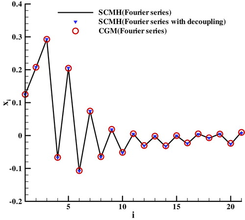
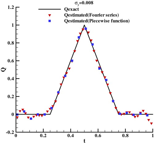
In this test case, dimensionless thermophysical properties and geometric parameters are set as ρ = 1, Cp = 1, T₀=0, k = 1, L = 0.2 and the measurement point is placed at z = L. The exact surface heat flux imposed at the left boundary are denoted as ‘Qexact’ in Figure 2, and some white noises whose standard deviations is σ = 0.008 are added to the exact temperature at the measurement point to simulate the measurement data. The measurement data is used to estimate the heat flux by using SCMH algorithm. For the piecewise linear function, the time range is divided into 20 uniform segments. For the Fourier series, first ten low-frequency components of the heat flux are retained as the estimation parameters, which means there are 21 unknown parameters to be estimated. The Markov chain length was set as 20,000 for the Fourier series as it is set as 50,000 for the piecewise linear function, and the first 10,000 points were rejected as the burn-in phase.

For comparison, the conjugated gradient method (CGM) is used to estimate the coefficients of the piecewise linear function and Fourier series. The heat fluxes estimated by the adaptive SCMH method presented in section 3.4 and CGM method are all shown in Figures 2–4. Because of the added white noise, there are some oscillations in the estimated heat flux, and the frequencies of oscillations are consistent in the two basis functions, which demonstrate that the two basis functions with the same number of parameters have consistent frequency resolution. The results of the adaptive SCMH and the adaptive SCMH with decoupling are in agreement with the results of the CGM, which demonstrates that the adaptive SCMH is viable and comparable with CGM.

Figure 2. The heat flux estimated with Piecewise function.

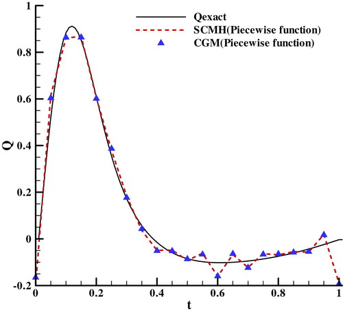
Figure 3. The heat flux estimated with Fourier series.

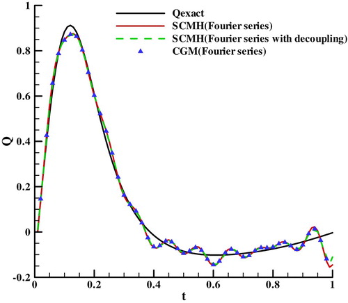
Figure 4. Fourier coefficients estimated by different methods.

The adaptive SCMH convergence processes of the parameter x₂ are presented in Figure 5. Although the parameters of the piecewise linear function and the Fourier series are different, the convergence processes of the two basis functions can basically reflect the convergence properties of that. It can be seen from Figure 5 that the convergence speed of the Fourier series is faster than that of the piecewise linear function. It also can be seen in the convergence processes of the piecewise linear function that the parameter has a long period oscillation and the more samples are needed to obtain the posterior distribution with the same accuracy. So Markov chain length needs to be set as 50,000 to reach equilibrium for the piecewise linear function in the test case.

Figure 5. Convergence process of different methods.

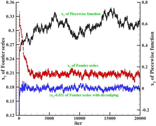
For validating the decoupling method, convergence processes of the parameter x₂ of the decoupling method are also shown in Figure 5. It can be seen that the Fourier series decoupling method presented in section 3.3 can successively shorten the burn-in period.

For investigating the adaptability of the two basis functions, a triangle heat flux shown as ‘Qexact’ in Figure 6 is loaded to the left boundary, the temperatures are also added with white nose, whose standard deviation is σ = 0.008, to simulate the measurement data. The results of estimation are shown in Figure 6. It can be seen that the heat flux estimated with the two basis functions are consistent and agreed with the true value, which manifest that piecewise linear function and Fourier series can be easily used to parameterize the different kinds of heat flux.

Figure 6. The triangle heat flux estimated with noises.

4.2. Comparison between piecewise function and Fourier series

According to Figures 2, 3 and 6 in section 4.1, it can be seen that the precision of heat flux estimated with piecewise function and Fourier series is consistent. Not only the mean value but also the variance of posterior distribution is the important indicator of the accuracy of the estimation results. Then all samples of the Fourier coefficients are converted to the quantities of the heat flux at every discrete time steps to obtain the posterior distribution of the heat flux in time domain, and the variances of the heat flux are shown in Figure 7. The results show that the variances converted from Fourier coefficients are obviously smoother than the variances of the heat flux converted from piecewise linear function. It should be concerned that the peaks in Figure 7 are located at the original points of piecewise linear function. This is because the heat flux can be expressed as Equation (12) with parameters of piecewise linear function when t is between t_i and t_i+1. (12) $Q\left(t\right)=\alpha x_i+(1-\alpha )x_{i+1}$(12) And then variance of heat flux can be written as (13) $D\left(Q\right(t\left)\right)={\alpha }^{2}D\left(x_i\right)+(1-\alpha {)}^{2}D\left(x_{i+1}\right)+2\text{Cov}(\alpha x_i,(1-\alpha \left)x_{i+1}\right)$(13)

Figure 7. The variances of posterior distribution of heat flux.

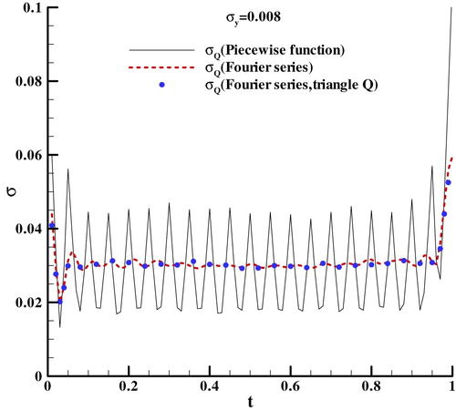
And in this test case, the adjacent parameters are negative correlated in sampling, which means $\text{Cov}(\alpha x_i,(1-\alpha \left)x_{i+1}\right)$ is minus, the follow equation can be derived from Equation (13). (14) $D\left(Q\right(t\left)\right)\le max\left(D\right(x_i),D(x_{i+1}\left)\right)\mathrm{a}\mathrm{n}\mathrm{d}D\left(Q\right(t\left)\right)\le 0.5\text{avg}\left(D\right(x_i),D(x_{i+1}\left)\right)\text{when}\alpha =0.5$(14) So the variances of the heat flux converted from piecewise linear function have some fluctuations and some peaks at the original point of piecewise linear function.

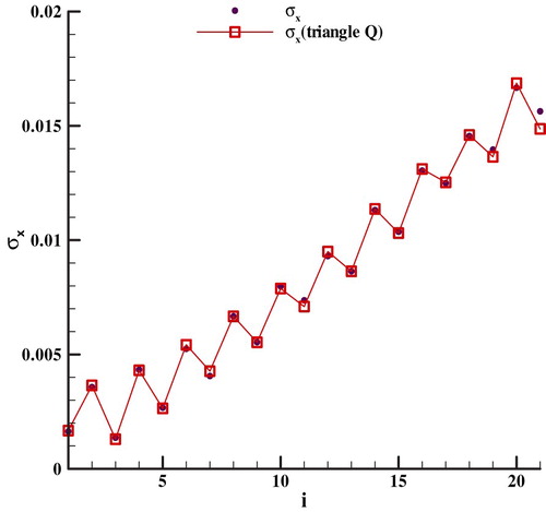
The variances of Fourier coefficients shown in Figure 8 increase with the frequency, which demonstrate that the errors of estimated heat flux also increase with the frequency.

Figure 8. The variances of posterior distribution of Fourier coefficients.

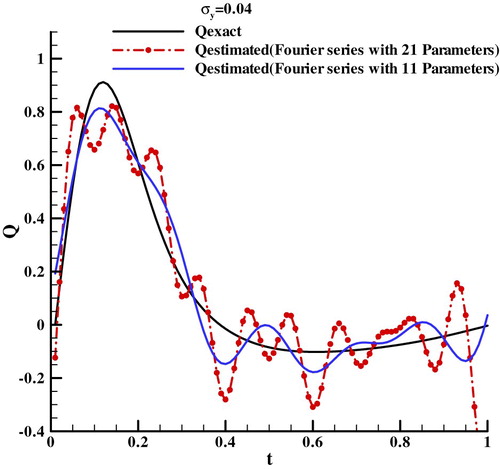
Furthermore, the exact temperatures are added with different white noises to simulate the measurement data, whose standard deviations are σ = 0.02, 0.04 and 0.08. And one group of the above estimation results with greater noises are shown in Figure 9. For reducing the oscillation of the heat flux in the high-frequency, the low-frequency components of heat flux are retained as the estimation parameters as the high frequency are removed. So it can be seen from Figure 9 that the estimation results with 11 parameters are smoother.

Figure 9. The heat flux estimated with greater noises.

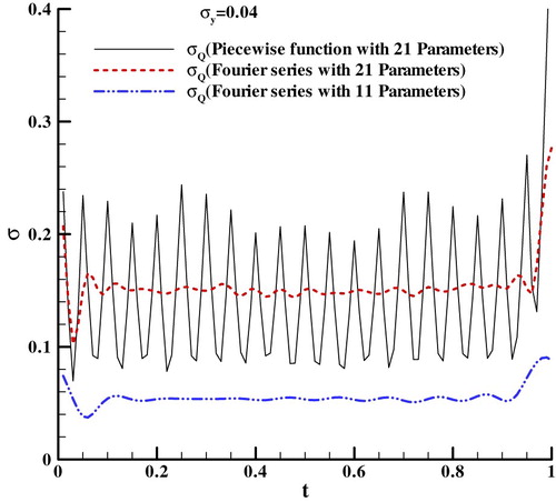
The variances of the heat flux are shown in Figure 10. It is the same as above case that the variances converted from Fourier coefficients are obviously smoother than the variances of the piecewise linear function coefficients. And the variances of the heat flux with 11 parameters are obviously smaller than 21 parameters, which is because the variances of high-frequency components are also eliminated as the high-frequency components are removed. It is well known that the errors of estimated results come from the modelling errors and the measurement errors. So for obtaining good estimated results, the modelling errors and the influence of measurement errors should be balanced by choosing regularization parameter.

Figure 10. The variances of posterior distribution of heat flux with greater noises.

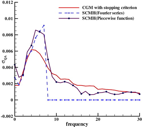
For ill-posed problem, the regularization parameter has a great impact on the identification results; in this case the number of unknown coefficients can be regarded as a regularization parameter. The average estimation heat flux errors of 64 samples were calculated to find optimal regularization parameter. For comparison, the average estimation errors of piecewise function and Fourier series with optimal regularization parameter and CGM with stopping criterion are shown in Figure 11. The results denote that SCMH with piecewise function and Fourier series show a similar performance while CGM performs relatively poorly. It’s well known that stopping criterion which is an Alifanov’s iterative regularization method [3] can stabilize the solution, it works like a filter. For finding filter performance of these methods and inspired by reference [24,25], the standard deviation of 256 sets of the estimation heat flux in frequency domain is shown in Figure 12, which can reflect how these methods to suppress high-frequency oscillation. This figure demonstrates that the three methods are essentially low-pass filters but with different performance.

Figure 11. The estimation errors of different methods.

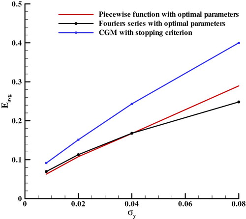
Figure 12. The standard deviation of the estimation heat flux in frequency domain.

The sampling efficiency of the adaptive SCMH with these two basis functions should be concerned. In section 4.1, it can be seen that the parameters of piecewise function have a longer period oscillation than that of Fourier series in the sample process. The highly correlation of parameters leads to larger search space and lower algorithm efficiency. The sensitivity of the parameters can be calculated by sensitivity function, and the cross-correlation coefficients of the sensitivity can be used to scale the correlation of unknown parameters. Then the cross-correlation coefficients of the sensitivity of first 5 parameters are presented in Table 1. The results show that:

1. The adjacent parameters of piecewise linear function are strongly correlated, and the correlation decrease with the increasing of the distance between parameters.

2. The first two parameters of Fourier series are strongly correlated as the other parameters are slightly correlated.

Table 1. Cross-correlation of coefficients of the sensitivity.

Piecewise linear function	x1	x2	x3	x4	x5
x1	1.000	0.552	0.184	−0.083	−0.395
x2	0.552	1.000	0.842	0.580	0.355
x3	0.184	0.842	1.000	0.856	0.623
x4	−0.083	0.580	0.856	1.000	0.832
x5	−0.395	0.355	0.623	0.832	1.000
Fourier series	x1	x2	x3	x4	x5
x1	1.000	−0.771	0.066	−0.278	−0.018
x2	−0.771	1.000	−0.026	−0.106	0.046
x3	0.066	−0.026	1.000	0.051	−0.001
x4	−0.278	−0.106	0.051	1.000	0.004
x5	−0.018	0.046	−0.001	0.004	1.000

Furthermore, average squared jumping distances divided by the variances of parameters can be used as normalized average squared jumping distances to compare the efficiency of the two basis functions. Then the normalized average squared jumping distances of first 5 parameters are presents in Table 2. The results show that

1. The normalized average squared jumping distances of parameters of Fourier series is greater than that of Piecewise linear function, which means the adaptive SCMH algorithm with Fourier series is more efficient.

2. The normalized average squared jumping distances of the first two parameters of Fourier series is obviously smaller than that of other parameters, which is consistent with cross-correlation of coefficients presented in Table 1.

Table 2. Normalized average squared jumping distances.

Piecewise linear function	Aver sq Dist/Var(xi)	Acceptance rate
x1	6.26E−03	0.449
x2	2.55E−03	0.446
x3	4.25E−03	0.449
x4	4.70E−03	0.448
x5	4.67E−03	0.450
Fourier series	Aver sq Dist/Var(xi)	Acceptance rate
x1	1.46E−02	0.449
x2	8.39E−02	0.453
x3	0.244	0.453
x4	0.258	0.450
x5	0.243	0.447

In consideration of the correlation of parameters and the average squared jumping distances scaled with the variances of parameters, the Fourier series is more suitable than piecewise linear function for SCMH algorithm.

4.3. A comparison with ‘optimal’ variance method

In this case, the adaptive SCMH is also compared with ‘optimal’ variance algorithm presented in the reference [22]. As mentioned in section 3.4, because of correlation, 2.38² times of the variance of the component may be not optimal for SCMH. So for proving that, both ‘optimal’ variance algorithm with Fourier series and piecewise function are used to solve the test case presented in section 4.1, and average squared jumping distances of the adaptive SCMH and ‘optimal’ variance algorithm are computed and used to indicate efficiency. At the same time, many different variance of the proposal distribution are used in the standard SCMH to search optimal efficiency. Then average squared jumping distances of these standard SCMH and the adaptive SCMH are shown in Figures 13–14.

Figure 13. Efficiency of the first component of piecewise function.

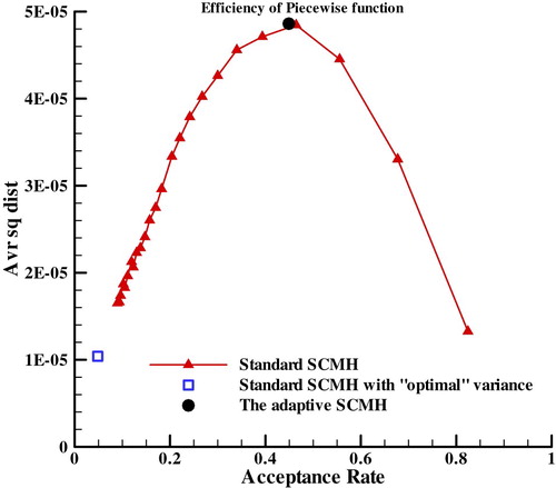
Figure 14. Efficiency of the first component of Fourier series.

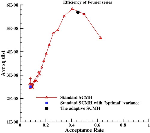
It can be seen that the average squared jumping distances of the adaptive SCMH are greater than the standard SCMH with ‘optimal’ variance and close to the optimal value, and the acceptance rate of the adaptive SCMH are also close to 0.45. Thus the adaptive method works well and can obviously improve the efficiency of SCMH.

4.4. Experimental result estimation

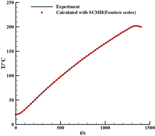
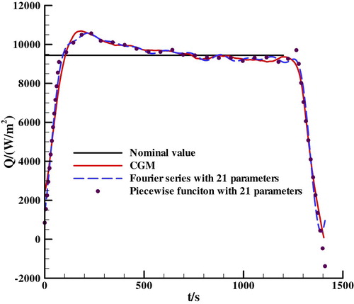
The estimation methods described in this paper and CGM are also applied to a principal experiment for IHCP [26]. In the experiment, the two samples of carbon-steel are heated by the electric heater which is sandwiched between two samples, a temperature history at the measurement point can be obtained with the thermocouple. The sample is 15 mm thick and the temperature measurement point is 6 mm from the heating surface. The heater worked for about 20 min, and temperature data were collected every 6 s for a total of 236 discrete points shown in Figure 15.

Figure 15. The comparison of experiment temperature and estimation result.

Considering the influence of the environment, the radiation and convective heat transfer should be taken into account in the calculation. So in the Formula (1), the boundary condition should be modified to the form below: $\text{At}z=0,-k\frac{\mathrm{\partial }T}{\mathrm{\partial }z}=Q\left(t\right);\text{at}z=L,-k\frac{\mathrm{\partial }T}{\mathrm{\partial }z}=\epsilon \delta (T^4-T_{\text{env}}^4)+h(T-T_{\text{env}})$

where $\epsilon$ is set to 0.85 and h is set to 5. The heat flux estimated with the SCMH and CGM are shown in Figure 16. The result shows that heat flux estimated with piecewise function and Fourier series is consistent and the estimated value of heat flux is very close to its nominal value, which reveals the feasibility of the SCMH to estimate heat flux.

Figure 16. The comparison of the test nominal value and the heat flux estimated by CGM and SCMH.

5. Conclusion

In this paper, the adaptive and decoupling SCMH sampling algorithm is presented to estimate the surface heat flux expressed by two different basis functions, the piecewise linear function and the Fourier series. The SCMH algorithm is validity by a numerical test case, and the decoupling methods are proven to be able to obviously shorten the burn-in period, the efficiency of the adaptive method is close to optimal as the components samples are correlated.

It also can be found that the algorithm with Fourier series is more efficient than that with piecewise linear function because of slighter correlation. It should be notified that the variances of heat flux converted from Fourier coefficients are obviously smoother than the variances of the piecewise linear function coefficients with same number of parameters. In addition, the number of parameters has similar influence as the regularization of the CGM, the fewer the parameters, the smoother the estimated heat flux. But how to build the precise relationship between the number of parameters and the regularization, it should be analysed in the future works.

Disclosure statement

No potential conflict of interest was reported by the authors.

Additional information

Funding

This work was supported by National Natural Science Foundation of China: [Grant Number 11372338]; Foundation of the State Key Laboratory of Aerodynamics: [Grant Number JBKY11030903].

References

- Beck JV, Blackwell B, Clair CR. Inverse heat conduction: ill-posed problems. New York (NY): Wiley Interscience; 1985.
- Raynaud M, Beck J V. Methodology for comparison of inverse heat conduction methods. J Heat Transfer. 1988;110:30–37.
- Alifanov OM. Inverse heat transfer problems. Berlin: Springer-Verlag; 1994.
- Taler J, Duda P. Experimental verification of space marching methods for solving inverse heat conduction problems. Heat Mass Transfer. 2000;36(4):325–331.
- Battaglia JL, Cois O, Puigsegur L, et al. Solving an inverse heat conduction problem using a non-integer identified model. Int J Heat Mass Transf. 2001;44:2671–2680.
- Monde M. Analytical method in inverse heat transfer problem using Laplace transform technique. Int J Heat Mass Transf. 2000;43:3965–3975.
- Qian WQ, He KF, Zhou Y. Estimation of surface heat flux for ablation and charring of thermal protection material. Heat Mass Transfer. 2016;52(7):1275–1281.
- Schmidt DM, George JS, Wood CC. Bayesian inference applied to the electromagnetic inverse problem. Hum Brain Mapp. 1999;7(3):195–212.
- Martin J, Wilcox LC, Burstedde C, et al. A stochastic Newton MCMC method for large-scale statistical inverse problems with application to seismic inversion. SIAM J Sci Comput. 2012;34(3):A1460–A1487.
- Beaumount MA, Balding DJ. Identifying adaptive genetic divergence among populations from genome scans. Mol Ecol. 2004;13(4):969–980.
- Mao SS. Bayesian statistic. Beijing: China Statistics Press; 1999;. Chinese.
- Battaglia JL, Fudym O, Orlande HRB, et al. Estimation of thermal parameters from picoseconds thermo reflectance. Paper presented at: IPDO2013; 2013 June 26–28; Albi, France.
- Orlande HRB, Dulikravich GS, Neumayer M, et al. Accelerated Bayesian inference for the estimation of spatially varying heat flux in a heat conduction problem. Numer Heat Transfer Part A: Appl. 2014;65(1):1–25.
- Wang JB, Zabaras N. A Bayesian inference approach to the inverse heat conduction problem. Int J Heat Mass Transf. 2004;47:3927–3941.
- Wang JB, Zabaras N. Hierarchical Bayesian models for inverse problems in heat conduction. Inverse Probl. 2005;21:183–206.
- Balaji C, Padhi T. A new ANN driven MCMC method for multi-parameter estimation in two-dimension conduction with heat generation. Int J Heat Mass Transf. 2010;53:5440–5455.
- Qian WQ, Cai JS. Parameter estimation of heat conduction coefficient and heat flux by sensitivity method. Acta Aerodynam Sin. 1998;16(2):226–231. Chinese.
- Haario H, Saksman E, Tamminen J. Componentwise adaptation for high dimensional MCMC. Comput Stat. 2005;20:265–273.
- Qian WQ, Zhou Y, Shao YP, et al. A preliminary analysis of identifiability of surface heat flux. J Exp Fluid Mech. 2013;27(4):17–22. Chinese.
- Elden L, Berntsson F, Reginska T. Wavelet and Fourier method for solving the sideways heat equation. Siam J Sci Comput. 2000;21(6):2187–2205.
- Cattani L, Maillet D, Bozzoli F, et al. Estimation of the local convective heat transfer coefficient in pipe flow using a 2D thermal quadrupole model and truncated singular value decomposition. Int J Heat Mass Transf. 2015;91:1034–1045.
- Roberts GO, Gelman A, Gilks WR. Weak convergence and optimal scaling of random walk Metropolis algorithms. Ann Appl Probab. 1997;7(1):110–120.
- Roberts GO, Rosenthal JS. Examples of adaptive MCMC. J Comput Graph Stat. 2009;18(2):349–367.
- Bozzoli F, Cattani F, Mocerino A, et al. A novel method for estimating the distribution of convective heat flux in ducts: Gaussian filtered singular value decomposition. Inverse Problem Sci Eng. 2019;27(11):1595–1607.
- Bozzoli F, Rainieri S. Comparative application of CGM and Wiener filtering techniques for the estimation of heat flux distribution. Inverse Probl Sci Eng. 2011;19(4):551–573.
- Qian WQ, Wu SJ, Bu HT, et al. Preliminary investigation of principle experiment for aerothermodynamic parameter estimation. J Exp Fluid Mech. 2009;23(3):59–62. Chinese.