An improved generalized flexibility matrix approach for structural damage detection

ABSTRACT

Structural damage detection is a key part of structural health monitoring. The generalized flexibility matrix approach is an effective method for damage detection. Compared with the flexibility matrix approach, it requires less number of natural frequencies and corresponding mode shapes. In this paper, the approach is improved by considering the nonnegativity of the damage extent. The error bound of two solutions calculated by the improved approach using natural frequencies and corresponding mode shapes without and with noises is derived. Numerical examples with different damage scenarios show that compared with the original generalized flexibility matrix approach, our proposed method works better.

KEYWORDS:

• Damage detection
• flexibility matrix
• natural frequency
• mode shape
• linear complementarity

AMS SUBJECT CLASSIFICATIONS:

• 70J10
• 90C33

1. Introduction

Many engineering structures such as bridges, tall buildings and offshore platforms are designed to have long life spans. During their service life-cycles, they may be subjected to the deterioration due to environmental influences, changes in load characteristics and some random actions [1]. These factors often result in structural damages. Damages are main causes of structural failure in mechanical structures [2]. If they cannot be found immediately, they will become more and more serious, and may lead to a disaster. Thus, detecting damages at the early stage is very important [3]. It is a key part of structural health monitoring [4].

Various detection methods have been proposed during the last few decades. Among these methods, a type of methods named vibration-based method has attracted much attention. Vibration-based method makes full use of the difference in dynamic features of the structure before and after the damage. Changes in natural frequencies, mode shapes and its curvatures, modal flexibility and its derivatives, modal strain energy and frequency response function can be utilized [5]. This type of method can present a global damage assessment, and detect damages which are not on the surface of the structure.

Changes in the first lower natural frequencies are frequently used in damage detection, because frequencies can be measured more easily and exactly than corresponding mode shapes. For example, Li et al. detected damages by the generalized flexibility matrix (GFM) and changes in natural frequencies [3]. Zhang et al. used changes in the first three natural frequencies to detect damages of continuum structures [6]. They presented a level set model, which can perfectly describe the shape of damage regions and can deal with damage regions with complex shapes. Based on the measured natural frequencies of structures, Wang et al. identified damages by interval analysis technique [7]. In addition, frequency response function has also been extensively used for damage detection [8–12]. Yu et al. used frequency response function and fuzzy clustering to diagnose damages of a six bay truss bridge [9]. Using frequency response function, Guo et al. transferred the identification problem to a nonlinear optimization problem whose objection function is the constitutive relation error [10].

Besides natural frequency, the vibration mode is fundamental and important in damage detection. It provides more abundant information than frequency. For example, Pandey et al. proposed the mode shape curvature method and successfully applied the method to detect damage in cantilever and simply supported beam [13]. The basic idea of their method is that changes in mode shape curvature at nodes related to damage elements are significant before and after the damage. Cao et al. utilized the improved form of the mode shape curvature to detect cracks in beams [14]. Yan and Ren derived the close form of the sensitivity of modal flexibility, and used it to detect damage locations and extents [15]. Seyedpoor and Montazer proposed a flexibility-based damage probability index and used it for damage identification [16]. Lu and Wang proposed an enhanced response sensitivity approach for structural damage detection [17]. Shahri and Ghorbani-Tanha used the closed-form sensitivity matrix of modal kinetic energy change ratio to detect the damage [18]. Hosseinzadeh et al. employed Neumann series expansion-based model reduction technique for damage identification with sparse sensor measurements [19]. Cui et al. proposed a damage detection method based on strain modes [20]. Bernagozzi et al. gave a detection method for buildings, their approach is based on modal flexibility deflections [21]. Dahak et al. presented a method for predicting the damage location and severity based on the frequency contour method [22]. The contour lines are plotted by the values of changes in measured frequencies and the curvature mode shapes of the intact structure. Their method is simpler than other similar methods. In addition, Ghadimi and Kourehli detected cracks in beam structures under moving mass using extreme learning machine and the least square support vector machine [23].

Besides above methods, some researchers presented two-stage method for damage detection [24–27]. This kind of method first locates potential damage elements by a damage indicator. Then, the extent of damage elements is achieved by solving an optimization problem. The number of optimization variables is equal to that of damage elements that are determined by the first step. Therefore, such an optimization problem is usually small in scale, and its solution is relatively easy.

In 2010, Li et al. first presented the definition of GFM [28]. The advantage of their method is that the effect of truncating higher-order modes can be reasonably reduced. Compared with the original flexibility matrix method [29,30], it requires less number of natural frequencies and corresponding mode shapes. Thus, the idea of the GFM has been extensively used for damage detection [3,28,31–33]. However, their method does not take into account the nonnegativity of the damage extent. In this paper, the approach is improved by considering the boundedness of the damage extent.

The remainder of the paper is organized as follows. In Section 2, the problem is formulated. The GFM approach (GFMA) is reviewed and our method is presented in Section 3. The error bound of two solutions calculated by our proposed method using natural frequencies and corresponding mode shapes without and with noises is derived in Section 4. Numerical examples are employed to illustrate the effectiveness of the method in Section 5 and conclusions are drawn in Section 6.

2. Preliminaries

2.1. Problem formulation

In this paper, it is assumed that the structural damage only results in a reduction of structural stiffness, the structural mass and the number of degrees of freedom (DOFs) remains unchanged. Under this assumption, the structural damage detection problem can be stated as follows [28]. Let ${\mathbf{K}}_u$ and ${\mathbf{K}}_d$ be the $n\times n$ global stiffness matrix of the undamaged and damaged structures, respectively. ${\mathbf{K}}_{ui}$ is the $n\times n$ stiffness matrix corresponding to the $i\text{th}$ element of the undamaged structure. Then, the matrix ${\mathbf{K}}_d$ can be expressed as follows (1) ${\mathbf{K}}_d={\mathbf{K}}_u-\mathrm{\Delta }\mathbf{K}$(1) where $\mathrm{\Delta }\mathbf{K}$ is the change of the global stiffness matrix. By the finite element method, $\mathrm{\Delta }\mathbf{K}$ is the summation of changes of some elemental stiffness matrices, i.e. (2) $\mathrm{\Delta }\mathbf{K}=\sum _{i=1}^m{\alpha }_i{\mathbf{K}}_{ui}$(2) where $m$ is the number of total elements of the structure, $0\le {\alpha }_i\le 1$ stands for the damage extent of the $i\text{th}$ element $(i=1,2,\dots ,m)$. ${\alpha }_i=0$ indicates that the $i\text{th}$ element is undamaged. Due to the inevitable measurement noise, small ${\alpha }_i$ may be produced even if the $i\text{th}$ element is intact. Thus, small ${\alpha }_i$ can not demonstrate that the $i\text{th}$ element is damaged. In this paper, the $i\text{th}$ element is regarded as a damaged one if ${\alpha }_i\ge 0.05$. The same limitation was also adopted in Ref. [28]. The purpose of structural damage detection is to find all damage locations and extents, i.e. calculate ${\alpha }_i$ $(i=1,2,\dots ,m)$ by using the measured data.

2.2. The definition of the vec operation

Definition 2.1

([34,35]): Let $\mathbf{C}$ be a matrix with size $m\times n$. Its column partitioning is (3) $\mathbf{C}=[{\mathbf{c}}_1,{\mathbf{c}}_2,\dots ,{\mathbf{c}}_n]$(3) Then $\text{vec}\left(\mathbf{C}\right)$ is an $mn$-by-1 vector obtained by stacking columns of $\mathbf{C}$, i.e. (4) $\text{vec}\left(\mathbf{C}\right)=[{\mathbf{c}}_1^{\text{T}},{\mathbf{c}}_2^{\text{T}},\dots ,{\mathbf{c}}_n^{\text{T}}{]}^{\text{T}}$(4) It can be observed that the vec operation is linear. In addition, the vec operation has the following property (5) $||\text{vec}\left(\mathbf{C}\right)|{|}_2=||\mathbf{C}|{|}_{\text{F}}$(5) The above equation can be easily verified by definition 1.

3. The improved GFMA

In this section, the existing GFMA is first reviewed [28]. Then, our proposed method is given.

3.1. The GFMA

Substituting Equation (2) into Equation (1), and differentiating with respect to ${\alpha }_i$, we have (6) $\frac{\mathrm{\partial }{\mathbf{K}}_d}{\mathrm{\partial }{\alpha }_i}=-{\mathbf{K}}_{ui}$(6) Let ${\mathbf{F}}_d$ be the $n\times n$ flexibility matrix for the damaged structure, i.e. (7) ${\mathbf{F}}_d{\mathbf{K}}_d=\mathbf{I}$(7) where $\mathbf{I}$ is the $n\times n$ identity matrix. Differentiating Equation (7) with respect to ${\alpha }_i$ yields (8) $\frac{\mathrm{\partial }{\mathbf{F}}_d}{\mathrm{\partial }{\alpha }_i}{\mathbf{K}}_d+{\mathbf{F}}_d\frac{\mathrm{\partial }{\mathbf{K}}_d}{\mathrm{\partial }{\alpha }_i}=0$(8) Post-multiplying Equation (8) by ${\mathbf{F}}_d$ and substituting Equation (6) into it, we can obtain (9) $\frac{\mathrm{\partial }{\mathbf{F}}_d}{\mathrm{\partial }{\alpha }_i}={\mathbf{F}}_d{\mathbf{K}}_{ui}{\mathbf{F}}_d$(9) Based on the mode shape normalization with respect to the mass matrix, the GFM is introduced. It is defined as follows (10) ${\mathbf{f}}_d^g\left(\text{α}\right)={\mathbf{F}}_d(\mathbf{M}{\mathbf{F}}_d{)}^l={\mathbf{\Phi }}_d{\mathbf{\Lambda }}_d^{-1}{\mathbf{\Phi }}_d^{\text{T}}(\mathbf{M}{\mathbf{\Phi }}_d{\mathbf{\Lambda }}_d^{-1}{\mathbf{\Phi }}_d^{\text{T}}{)}^l={\mathbf{\Phi }}_d{\mathbf{\Lambda }}_d^{-1-l}{\mathbf{\Phi }}_d^{\text{T}}$(10) where $\mathbf{M}$ is the mass matrix, it remains unchanged before and after the damage, $\text{α}=({\alpha }_1,{\alpha }_2,\dots ,{\alpha }_m{)}^{\text{T}}$ is a vector consisting of the damage extent of all elements, ${\mathbf{\Phi }}_d$ and ${\mathbf{\Lambda }}_d$ are the mode shape matrix and diagonal matrix of natural frequency squared for the damaged structure, respectively. Equation (10) indicates that a larger $l$ can cause a reduced contribution of higher-order modes. For $l=0$, Equation (10) reduces to the original flexibility matrix, i.e. ${\mathbf{F}}_d={\mathbf{\Phi }}_d{\mathbf{\Lambda }}_d^{-1}{\mathbf{\Phi }}_d^{\text{T}}$. For $l=1$, the GFM in Equation (10) becomes (11) ${\text{f}}_d^g\left(\text{α}\right)={\mathbf{F}}_d\mathbf{M}{\mathbf{F}}_d={\mathbf{\Phi }}_d{\mathbf{\Lambda }}_d^{-1}{\mathbf{\Phi }}_d^{\text{T}}\mathbf{M}{\mathbf{\Phi }}_d{\mathbf{\Lambda }}_d^{-1}{\mathbf{\Phi }}_d^{\text{T}}={\mathbf{\Phi }}_d{\mathbf{\Lambda }}_d^{-2}{\mathbf{\Phi }}_d^{\text{T}}$(11) In this paper, only $l=1$ is used. Differentiating Equation (11) with respect to ${\alpha }_i$ yields (12) $\frac{\mathrm{\partial }{\mathbf{f}}_d^g}{\mathrm{\partial }{\alpha }_i}=\frac{\mathrm{\partial }{\mathbf{F}}_d}{\mathrm{\partial }{\alpha }_i}\mathbf{M}{\mathbf{F}}_d+{\mathbf{F}}_d\mathbf{M}\frac{\mathrm{\partial }{\mathbf{F}}_d}{\mathrm{\partial }{\alpha }_i}$(12) Substituting Equation (9) into Equation (12) and setting ${\alpha }_i=0$ $(i=1,2,\dots ,m)$, we get (13) ${\left.\frac{\mathrm{\partial }{\mathbf{f}}_d^g}{\mathrm{\partial }{\alpha }_i}\right|}_{{\alpha }_i=0}={\mathbf{F}}_u{\mathbf{K}}_{ui}{\mathbf{F}}_u\mathbf{M}{\mathbf{F}}_u+{\mathbf{F}}_u\mathbf{M}{\mathbf{F}}_u{\mathbf{K}}_{ui}{\mathbf{F}}_u$(13) where ${\mathbf{F}}_u$ is the $n\times n$ flexibility matrix corresponding to the undamaged structure. So far, sensitivity analysis of the GFM is achieved. In practice, the number of damaged elements is usually small compared with the number of structural elements, i.e. most components of $\text{α}$ are zeros. Even for the damage elements, the damage extent can not be very large in most cases, i.e. nonzero components of $\text{α}$ are not very large. Thus, ${\mathbf{f}}_d^g\left(\text{α}\right)$ in Equation (10) can be approximated by the first-order Taylor’s series expansion, i.e. (14) ${\mathbf{f}}_d^g\approx {\mathbf{f}}_u^g+\sum _{i=1}^m{\alpha }_i{\left.\frac{\mathrm{\partial }{\mathbf{f}}_d^g}{\mathrm{\partial }{\alpha }_i}\right|}_{{\alpha }_i=0}$(14) Combining (13) and (14), we have (15) $\mathrm{\Delta }\mathbf{f}={\mathbf{f}}_d^g-{\mathbf{f}}_u^g\approx \sum _{i=1}^m{\alpha }_i({\mathbf{F}}_u{\mathbf{K}}_{ui}{\mathbf{F}}_u\mathbf{M}{\mathbf{F}}_u+{\mathbf{F}}_u\mathbf{M}{\mathbf{F}}_u{\mathbf{K}}_{ui}{\mathbf{F}}_u)=\sum _{i=1}^m{\alpha }_i{\mathbf{C}}_i$(15) where ${\mathbf{f}}_u^g={\mathbf{f}}_d^g\left(0\right)={\mathbf{F}}_u\mathbf{M}{\mathbf{F}}_u$, $\mathrm{\Delta }\mathbf{f}$ is the change of the GFM, and (16) ${\mathbf{C}}_i={\mathbf{F}}_u{\mathbf{K}}_{ui}{\mathbf{F}}_u\mathbf{M}{\mathbf{F}}_u+{\mathbf{F}}_u\mathbf{M}{\mathbf{F}}_u{\mathbf{K}}_{ui}{\mathbf{F}}_u(i=1,2,,m).$(16) Equation (11) indicates that the GFM can be approximated by only a few of lower frequency modes. Thus, (17) $\mathrm{\Delta }\mathbf{f}={\mathbf{F}}_d\mathbf{M}{\mathbf{F}}_d-{\mathbf{F}}_u\mathbf{M}{\mathbf{F}}_u\approx \sum _{j=1}^p\frac{1}{{\omega }_{dj}^4}{\mathbf{\Phi }}_{dj}{\mathbf{\Phi }}_{dj}^{\text{T}}-\sum _{j=1}^p\frac{1}{{\omega }_{uj}^4}{\mathbf{\Phi }}_{uj}{\mathbf{\Phi }}_{uj}^{\text{T}}$(17) where $p$ is the number of measured modes, ${\omega }_{dj}$ and ${\mathbf{\Phi }}_{dj}$ are the $j\text{th}$ smallest frequency and corresponding mode shape for the damaged structure, ${\omega }_{uj}$ and ${\mathbf{\Phi }}_{uj}$ are the $j\text{th}$ smallest frequency and corresponding mode shape for the undamaged structure. Combining (15) and (17), and ignoring the error, we have (18) $\sum _{i=1}^m{\alpha }_i{\mathbf{C}}_i=\mathbf{\Delta }\mathit{f}$(18) By vec operation, the above equation can be transferred to be a linear system with $n^2$ equations and $m$ unknowns, that is (19) $\sum _{i=1}^m{\alpha }_i\text{vec}\left({\mathbf{C}}_i\right)=\text{vec}\left(\mathbf{\Delta }\mathit{f}\right)$(19) Equation (19) can be written as (20) $\mathbf{A}\alpha =\mathbf{b}$(20) where $\mathbf{A}=\left[\text{vec}\left({\mathbf{C}}_1\right),\text{ vec}\left({\mathbf{C}}_2\right),\dots ,\text{vec}\left({\mathbf{C}}_m\right)\right]\in R^{n^2\times m}$, and $\mathbf{b}=\text{vec}\left(\mathbf{\Delta }\mathit{f}\right)\in R^{n^2}$. Solving the linear system (20) by the least square method, both damage locations and extents can be achieved.

3.2. Our proposed method

As has been said in Section 2, the damage extent of the $i\text{th}$ element should be nonnegative, i.e. $0\le {\alpha }_i\le 1$ $(i=1,2,,m)$. However, the above GFMA does not consider this property of damage extents. In this paper, the following optimization model is employed for the damage detection (21) $\begin{array}{rl}& \underset{\text{α}}{min}||\mathbf{b}-\mathbf{A}\alpha |{|}_2^2\\ & \text{s.t.}0\le {\alpha }_i\le \text{1}(i=1,2,,m)\end{array}$(21) This is a bound-constrained least square (BLS) problem. As to the method of solving this problem, we refer readers to Refs. [36–38].

4. The error bound of two solutions calculated by our proposed method using the measured data without and with noise

During the process of the structural dynamic test, measured natural frequencies and corresponding mode shapes are often contaminated. In this section, the error bound of two solutions calculated by our proposed method using the measured data without and with noise is presented. For this purpose, the linear complementarity problem (LCP) is first reviewed.

The LCP is to calculate a vector $\mathbf{x}\in R^k$ such that (22) $\mathbf{B}x+\mathbf{q}\ge \mathbf{0},\mathbf{x}\ge \mathbf{0}\text{and}{\mathbf{x}}^{\text{T}}(\mathbf{B}x+\mathbf{q})=\mathbf{0}$(22) where $\mathbf{B}\in R^{k\times k}$, $\mathbf{q}\in R^k$, and the notation ‘$\ge$’ represents the componentwise defined partial ordering between two vectors. In the following, problem (22) and its solution are denoted by LCP ($\mathbf{B},\mathbf{q}$) and $\mathbf{x}(\mathbf{B},\mathbf{q})$, respectively. Many problems in scientific computing and engineering applications need to solve the LCP. For example, the market equilibrium problem, the contact problem and the Nash equilibrium point problem of a bimatrix game are eventually transformed into LCPs [39,40]. In addition, the LCP also constitutes the Karush-Kuhn-Tucker optimality condition of the quadratic programming problem. Let’s consider the following the quadratic programming problem: (23) $\begin{array}{ll}min& f\left(\mathbf{x}\right)=\frac{1}{2}{\mathbf{x}}^{\text{T}}\mathbf{D}x+{\mathbf{c}}^{\text{T}}\mathbf{x}\\ \text{s}\text{.t}\text{.}& \mathbf{H}x\ge \mathbf{g}\\ & \mathbf{x}\ge \mathbf{0}\end{array}$(23) where $\mathbf{H}\in R^{s\times k}$, $\mathbf{D}\in R^{k\times k}$ is a symmetric matrix. Then, we have the following result.

Lemma 4.1

([39]): Let $\tilde{\mathbf{x}}\in R^k$ be the solution of problem (23). Then, there exist vector $\tilde{\mathbf{y}}\in R^s$ and slack vectors $\tilde{\mathbf{u}}\in R^k,\tilde{\mathbf{v}}\in R^s$ such that $\tilde{\mathbf{x}},\tilde{\mathbf{y}},\tilde{\mathbf{u}},\tilde{\mathbf{v}}$ together satisfy (24) $\begin{array}{rl}& \left(\begin{array}{c}\tilde{\mathbf{u}}\\ \tilde{\mathbf{v}}\end{array}\right)-\left(\begin{array}{cc}\mathbf{D}& -{\mathbf{H}}^{\text{T}}\\ \mathbf{H}& \mathbf{0}\end{array}\right)\left(\begin{array}{c}\tilde{\mathbf{x}}\\ \tilde{\mathbf{y}}\end{array}\right)=\left(\begin{array}{c}\mathbf{c}\\ \mathbf{g}\end{array}\right)\\ & \left(\begin{array}{c}\tilde{\mathbf{u}}\\ \tilde{\mathbf{v}}\end{array}\right)\ge \mathbf{0},\left(\begin{array}{c}\tilde{\mathbf{x}}\\ \tilde{\mathbf{y}}\end{array}\right)\ge \mathbf{0}\mathrm{a}\mathrm{n}\mathrm{d}{\left(\begin{array}{c}\tilde{\mathbf{u}}\\ \tilde{\mathbf{v}}\end{array}\right)}^{\text{T}}\left(\begin{array}{c}\tilde{\mathbf{x}}\\ \tilde{\mathbf{y}}\end{array}\right)=0\end{array}$(24) i.e. $\left(\begin{array}{c}\tilde{\mathbf{x}}\\ \tilde{\mathbf{y}}\end{array}\right)$ is the solution of LCP$\left(\left(\begin{array}{cc}\mathbf{D}& -{\mathbf{H}}^{\text{T}}\\ \mathbf{H}& \mathbf{0}\end{array}\right),\left(\begin{array}{c}\mathbf{c}\\ \mathbf{g}\end{array}\right)\right)$.

Some theoretical analyses and algorithms for the LCP have already been proposed [39–41]. Several results related to our problem are given as follows.

Lemma 4.2

([40]): If $\mathbf{B}\in R^{k\times k}$ is a symmetric positive definite (SPD) matrix, then for any $\mathbf{q}\in R^k$, the LCP ($\mathbf{B},\mathbf{q}$) has a unique solution.

Lemma 4.3

([41]): If $\mathbf{B}\in R^{k\times k}$ is a SPD matrix, $\mathbf{p},\mathbf{q}\in R^k$, then $||\mathbf{x}(\mathbf{B},\mathbf{p})-\mathbf{x}(\mathbf{B},\mathbf{q})|{|}_2\le ||{\mathbf{B}}^{-1}|{|}_2||\mathbf{p}-\mathbf{q}|{|}_2$

Lemma 4.4:

Let ${\mathbf{x}}^{\ast }\in R^m$ be the solution of the BLS problem (21). Then, there exists ${\mathbf{y}}^{\ast }\in R^m$ such that $\left(\begin{array}{c}{\mathbf{x}}^{\ast }\\ {\mathbf{y}}^{\ast }\end{array}\right)\in R^{2m}$ is the solution of LCP $\left(\left(\begin{array}{cc}{\mathbf{A}}^{\mathrm{T}}\mathbf{A}& \mathbf{I}\\ -\mathbf{I}& \mathbf{0}\end{array}\right),\left(\begin{array}{c}-{\mathbf{A}}^{\mathrm{T}}\mathbf{b}\\ -\mathbf{1}\end{array}\right)\right)$.

Proof:

See the appendix.

Theorem 4.1:

Assume $\mathbf{A}\in R^{s\times k}$, ${\mathbf{b}}_i\in R^s$. ${\mathbf{x}}_i$ is the solution of the following BLS problems $\underset{\mathbf{x}}{min}||{\mathbf{b}}_i-\mathbf{A}x|{|}_2,\text{ s}\text{.t}\text{. }\mathbf{0}\le \mathbf{x}\le \mathbf{1}$, $i=1,2$. Then, $||{\mathbf{x}}_1-{\mathbf{x}}_2|{|}_2\le \left(1+||\mathbf{A}|{|}_2^2\right)||\mathbf{A}|{|}_2||{\mathbf{b}}_1-{\mathbf{b}}_2|{|}_2$

Proof:

See the appendix.

The following theorem gives the error bound of two solutions calculated by natural frequencies and corresponding mode shapes without and with noise.

Theorem 4.2:

Assume ${\omega }_{dj}$ and ${\mathbf{\Phi }}_{dj}$ are the $j\text{th}$ smallest frequency and the corresponding mode shape of the damaged structure without noise, ${\omega }_{dj}+\mathrm{\Delta }{\omega }_{dj}$ and ${\mathbf{\Phi }}_{dj}+\mathrm{\Delta }{\mathbf{\Phi }}_{dj}$ are the $j\text{th}$ smallest frequency and the corresponding mode shape of the damaged structure with noise $(j=1,2,,p)$. ${\alpha }^{\ast }$ and ${\text{β}}^{\ast }$ are solutions of our proposed method calculated by the uncontaminated and contaminated measured data, respectively. Then, the following inequality holds $\begin{array}{rl}& ||{\text{α}}^{\ast }-{\text{β}}^{\ast }|{|}_2\le \left(1+||\mathbf{A}|{|}_2^2\right)||\mathbf{A}|{|}_2\\ & \times \sum _{j=1}^p\left[c_{dj}|\mathrm{\Delta }{\omega }_{dj}|||{\mathbf{\Phi }}_{dj}|{|}_2^2+\frac{{||\mathrm{\Delta }{\mathbf{\Phi }}_{dj}||}_{\text{2}}}{{({\omega }_{dj}+\mathrm{\Delta }{\omega }_{dj})}^4}(2{||{\mathbf{\Phi }}_{dj}||}_{\text{2}}+{||\mathrm{\Delta }{\mathbf{\Phi }}_{dj}||}_{\text{2}})\right]\end{array}$ where $c_{dj}$ is a positive number given in the following. (25) $c_{dj}=\frac{|2{\omega }_{dj}+\mathrm{\Delta }{\omega }_{dj}|(2{\omega }_{dj}^2+2{\omega }_{dj}\mathrm{\Delta }{\omega }_{dj}+\mathrm{\Delta }{\omega }_{dj}^2)}{{\omega }_{dj}^4{({\omega }_{dj}+\mathrm{\Delta }{\omega }_{dj})}^4}$(25)

Proof:

See the appendix.

Remark 4.1:

From the above theorem, it can be observed that for a given noise, the error bound of two solutions of our method is mainly determined by $\left(1+||\mathbf{A}|{|}_2^2\right)||\mathbf{A}|{|}_2$.

5. Numerical examples

In this section, two examples are presented to show the effectiveness of the proposed method, each example includes four damage scenarios. Here, damage is simulated by reducing the stiffness of specified elements. All BLS problems in these examples are solved by the command lsqlin in Matlab (R2016b).

Example 1: A hollow beam bridge model is studied in this example. The length and width of the bridge are $44\text{m}$ and $4\text{m}$, respectively. The size of the cross section is given in Figure 1. The bridge is simplified as a plane beam and is discretized into a finite element model with 22 elements and 23 nodes, as shown in Figure 2. Axial displacements of all nodes are ignored. Thus, every node has 2 DOFs except two constrained nodes. The total number of DOFs in the structure is 42. The material and geometric parameters are as follows: Young’s modulus $E=2.3\times {10}^{10}\text{Pa}$, Poisson’s ratio $\nu =0.167$, density $\rho =2300\text{kg}/{\text{m}}^3$, length $l=2\text{m}$, and second moment of area $I_z=0.5922{\text{m}}^4$. Four damage cases are considered, as shown in Table 1.

Figure 1. The size of the cross section of the hollow beam bridge.

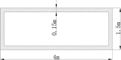
Figure 2. The simplified plane beam.

Table 1. Damage cases in Example 1.

Damage case		Damaged element(s)	Damage extent
Case 1	Single damage	Element 4	15%
Case 2	Double damage	Element 4	15%
		Element 9	10%
Case 3	Triple damage	Element 4	15%
		Element 9	10%
		Element 16	20%
Case 4	Multiple damage	Elements 4, 20	15%
		Element 9	10%
		Element 16	20%

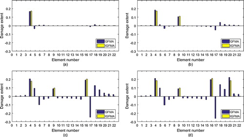
In this example, only the first frequency and the corresponding mode shape are employed to calculate damage locations and extents, i.e. solving the BLS problem (21) with $p=1$ to achieve ${\alpha }_i(1\le i\le 22)$. For comparison, damage locations and extents are also calculated by the GFMA with $p=1$, where GFMA is the abbreviation of generalized flexibility matrix approach. The results of two approaches are given in Figure 3. It can be observed that negative entries with larger absolute value are produced by the GFMA, which are opposed to the fact $0\le {\alpha }_i\le 1(1\le i\le 22)$. This is because GFMA does not consider the nonnegativity of damage extent. Our method utilizes the nonnegativity of damage extent and avoids this deficiency of the GFMA. In addition, for the last two damage cases, misjudgements for elements 18 and 19 are made by the GFMA. Our method, i.e. improved GFMA (IGFMA), does not produce the misjudgement.

Figure 3. Calculated results for all damage cases in Table 1: (a) Case 1; (b) Case 2; (c) Case 3; (d) Case 4.

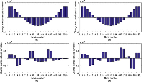
In addition, our method is compared with the mode shape curvature method. The mode shape curvature method detects damaged elements by changes in mode shape curvature of structural nodes before and after the damage. If the change in mode shape curvatures of a node is large, the element connected to this node is deemed as a damage one. The mode shape curvature in this paper is calculated by the central difference approximation. Figure 4 presents changes in mode shape curvatures of every node for all damage cases in Table 1. From Figure 4, it can be observed that the mode shape curvature method can exactly find damage locations for the last two damage cases. For the first two damage cases, it cannot give the right results. In addition, the method cannot provide damage extents.

Figure 4. Mode shape curvatures for all damage cases in Table 1: (a) Case 1; (b) Case 2; (c) Case 3; (d) Case 4.

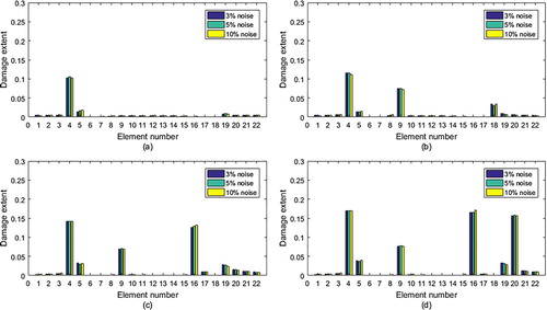
Our method has been carried out in the noise environment. The noise level of the natural frequency is $0.5\mathrm{\%}$, and the corresponding mode shape are contaminated with $3\mathrm{\%}$, $5\mathrm{\%}$, and $10\mathrm{\%}$ random noises. The assumed noise environment is produced by following formulas [18,42]: (26) $\begin{array}{rl}{\overline{\omega }}_d^{\ast }& ={\omega }_d^{\ast }(1+r\rho )\end{array}$(26) (27) $\begin{array}{rl}{\overline{\mathbf{\Phi }}}_{dj}^{\ast }& ={\mathbf{\Phi }}_{dj}(1+r_j\tilde{\rho }|{\varphi }_{max}|)\end{array}$(27) where ${\omega }_d^{\ast }$ and ${\overline{\omega }}_d^{\ast }$ are natural frequencies of the damaged structure without and with noise, $r$ and $r_j$ are Gaussian random numbers with mean $0$ and variance $1$, $\rho$ and $\tilde{\rho }$ are noise levels of the natural frequency and the mode shape, respectively. ${\mathbf{\Phi }}_{dj}$ and ${\overline{\mathbf{\Phi }}}_{dj}^{\ast }$ are the $j\text{th}$ components of mode shapes of the damaged structure without and with noise, and $|{\varphi }_{max}|$ is the largest absolute value among mode shape components. For every noise level, the contaminated natural frequency and the corresponding mode shape are produced by Equations (26) and (27). Subsequently, our method is implemented using each group of contaminated data to achieve the damage extent vector $\text{α}$. The procedure is repeated 1000 times. The mean value vector $\overline{\text{α}}$ is obtained by the above 1000 calculated damage extent vectors. Figure 5 presents the mean value vectors for all damage cases in Table 1. It can be seen that the IGFMA works well for these three noise levels.

Figure 5. Calculated results for all damage cases in Table 1 with three level noises: (a) Case 1; (b) Case 2; (c) Case 3; (d) Case 4.

Example 2: Consider a three-span beam structure as shown in Figure 6. The structure has 24 elements and 25 nodes and its length is $24\text{m}$. The cross section of the beam is square, and its size is $0.1\text{m}\times 0.1\text{m}$. Axial displacements of all nodes are ignored. Thus, every node has 2 DOFs except four constrained nodes. The two intermediate nodes are only constrained by the vertical direction, and each of them has 1 DOF. The total number of structural DOFs is 44. The material and geometric parameters of each element are as follows: Young’s modulus $E=3\times {10}^{10}\text{Pa}$, Poisson’s ratio $\nu =0.3$, density $\rho =2500\text{kg}/{\text{m}}^3$, length $l=1\text{m}$, and second moment of area $I_z=8.33\times {10}^{-6}{\text{m}}^4$. Four damage cases are considered, as shown in Table 2.

Figure 6. A three-span beam structure.

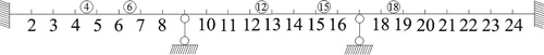
Table 2. Damage cases in Example 2.

Damage case		Damaged elements	Damage extent
Case 1	Double damage	Element 4	15%
		Element 6	20%
Case 2	Triple damage	Element 4	15%
		Element 6	20%
		Element 12	10%
Case 3	Multiple damage	Elements 4, 15	15%
		Element 6	20%
		Element 12	10%
Case 4	Multiple damage	Elements 4, 15	15%
		Elements 6, 18	20%
		Element 12	10%

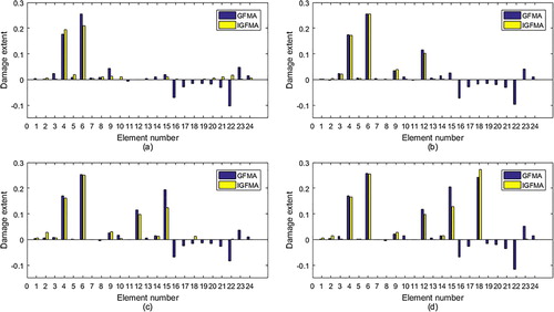
In this example, damage locations and extents are achieved by using first two frequencies and corresponding mode shapes. Calculated results of GFMA and IGFMA are listed in Figure 7. It can be observed that GFMA produces negative entries with larger absolute value. It also gives the misjudgement for element 23 for the first and last cases. These two shortcomings are overcome by the present method.

Figure 7. Calculated results for four damage cases in Table 2: (a) Case 1; (b) Case 2; (c) Case 3; (d) Case 4.

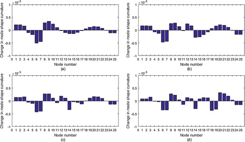
Our proposed method is also compared with the mode shape curvature method. Figure 8 gives changes in mode shape curvatures of every node for all damage cases in Table 2. It can be seen that the mode shape curvature method does not work well.

Figure 8. Mode shape curvatures for all damage cases in Table 1: (a) Case 1; (b) Case 2; (c) Case 3; (d) Case 4.

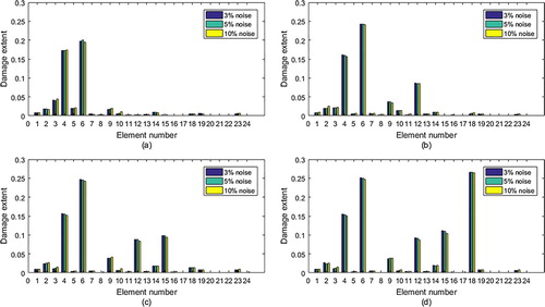
The IGFMA has been carried out in the noise environment. The method of imposing the noise and the noise level are the same as those in Example 1, see Equations (26) and (27). For every noise level, 1000 calculations have been done by the IGFMA. Then, the mean value vector for 1000 calculated damage extent vectors are computed. Figure 9 gives mean value vectors for all damage cases in Table 2. It can be seen that the IGFMA can also work for these three noise levels.

Figure 9. Calculated results for four damage cases in Table 2 with three level noises: (a) Case 1; (b) Case 2; (c) Case 3; (d) Case 4.

From these two examples, it can be observed that our proposed method can successfully identify the damaged locations, even in the presence of noise. In addition, the damage extent is simultaneously achieved. Our method is superior to the GFMA and mode shape curvature method.

6. Conclusions

The IGFMA is presented for structural damage detection problem. It is based on the GFM. The boundedness of the damage extent is considered and a BLS model is used. Thus, damage extents calculated by our method are all between 0 and 1. This is consistent with the fact. In addition, the perturbation theory of LCP is utilized to derive the error bound of two solutions calculated by the IGFMA using natural frequencies and corresponding mode shapes without and with noise. Part of our result (Theorem 4.1) can be applied to other detection approaches related to the BLS problem, so that the error bound of two solutions calculated by the corresponding approach using the measured data without and with noise can also be achieved.

The proposed method has been verified by numerical experiments with different damage scenarios. The calculated results show that the method can exactly find locations and extents of damage elements using only a few frequencies and mode shapes. This is an advantage of our method. When the data is with noise, our method also work. Compared with the GFMA and mode shape curvature method, our approach can achieve more accurate results and reduce the number of misjudgements. The future work is to generalize the proposed method to damage detection problem with incomplete mode shapes.

Disclosure statement

No potential conflict of interest was reported by the authors.

Additional information

Funding

The work was supported by the Natural Science Foundation of China [grant numbers 11672118 and 11401463].

Appendix

Proof

Proof of lemma 4.4

It is easy to verify that the BLS problem (21) is equivalent to following quadratic programming problem: $\begin{array}{rl}& minf\left(\mathbf{x}\right)=\frac{1}{2}{\text{α}}^{\text{T}}{\mathbf{A}}^{\text{T}}\mathbf{A}\alpha -{\mathbf{b}}^{\text{T}}\mathbf{A}\alpha \\ & \text{s}\text{.t}\text{.}\mathbf{0}\le \text{α}\le \mathbf{1}\end{array}$ In Lemma 4.1, let $\mathbf{D}={\mathbf{A}}^{\text{T}}\mathbf{A},\mathbf{c}=-{\mathbf{A}}^{\text{T}}\mathbf{b},\mathbf{H}=-\mathbf{I},\mathbf{g}=-\mathbf{1}$, the conclusion is achieved.

Proof

Proof of theorem 4.1

By Lemma 4.1, there exit ${\mathbf{y}}_i\in R^k$ such that $\left(\begin{array}{c}{\mathbf{x}}_i\\ {\mathbf{y}}_i\end{array}\right)\in R^{2k}$ is the solution of LCP$\left(\left(\begin{array}{cc}{\mathbf{A}}^{\text{T}}\mathbf{A}& \mathbf{I}\\ -\mathbf{I}& \mathbf{0}\end{array}\right),\left(\begin{array}{c}-{\mathbf{A}}^{\text{T}}{\mathbf{b}}_i\\ -\mathbf{1}\end{array}\right)\right)$, $i=1,2$. From Lemma 4.3, we have $\begin{array}{rl}||{\mathbf{x}}_1-{\mathbf{x}}_2|{|}_2& \le {∥\left(\begin{array}{c}{\mathbf{x}}_1\\ {\mathbf{y}}_1\end{array}\right)-\left(\begin{array}{c}{\mathbf{x}}_2\\ {\mathbf{y}}_2\end{array}\right)∥}_2\\ & \le {∥{\left(\begin{array}{cc}{\mathbf{A}}^{\text{T}}\mathbf{A}& \mathbf{I}\\ -\mathbf{I}& \mathbf{0}\end{array}\right)}^{-1}∥}_2{∥\left(\begin{array}{c}-{\mathbf{A}}^{\text{T}}{\mathbf{b}}_1\\ -\mathbf{1}\end{array}\right)-\left(\begin{array}{c}-{\mathbf{A}}^{\text{T}}{\mathbf{b}}_2\\ -\mathbf{1}\end{array}\right)∥}_2\\ & ={∥\left(\begin{array}{cc}\mathbf{0}& -\mathbf{I}\\ \mathbf{I}& {\mathbf{A}}^{\text{T}}\mathbf{A}\end{array}\right)∥}_2||{\mathbf{A}}^{\text{T}}({\mathbf{b}}_1-{\mathbf{b}}_2)|{|}_2\\ & \le \left({∥\left(\begin{array}{cc}\mathbf{0}& -\mathbf{I}\\ \mathbf{I}& \mathbf{0}\end{array}\right)∥}_2+{∥\left(\begin{array}{cc}\mathbf{0}& \mathbf{0}\\ \mathbf{0}& {\mathbf{A}}^{\text{T}}\mathbf{A}\end{array}\right)∥}_2\right)||{\mathbf{A}}^{\text{T}}|{|}_2||{\mathbf{b}}_1-{\mathbf{b}}_2|{|}_2\\ & =\left(1+{||{\mathbf{A}}^{\text{T}}\mathbf{A}||}_2\right)||\mathbf{A}|{|}_2||{\mathbf{b}}_1-{\mathbf{b}}_2|{|}_2\\ & =\left(1+||\mathbf{A}|{|}_2^2\right)||\mathbf{A}|{|}_2||{\mathbf{b}}_1-{\mathbf{b}}_2|{|}_2\end{array}$

Proof

Proof of theorem 4.2

For cases without and with noise, from (17), two right hands of our proposed method are related to following two matrices, respectively. $\begin{array}{rl}\mathrm{\Delta }\mathbf{g}& =\sum _{j=1}^p\frac{1}{{\omega }_{dj}^4}{\mathbf{\Phi }}_{dj}{\mathbf{\Phi }}_{dj}^{\text{T}}-\sum _{j=1}^p\frac{1}{{\omega }_{uj}^4}{\mathbf{\Phi }}_{uj}{\mathbf{\Phi }}_{uj}^{\text{T}}\end{array}$ $\begin{array}{rl}\mathrm{\Delta }\tilde{\mathbf{g}}& =\sum _{j=1}^p\frac{1}{{({\omega }_{dj}+\mathrm{\Delta }{\omega }_{dj})}^4}({\mathbf{\Phi }}_{dj}+\mathrm{\Delta }{\mathbf{\Phi }}_{dj})({\mathbf{\Phi }}_{dj}+\mathrm{\Delta }{\mathbf{\Phi }}_{dj}{)}^{\text{T}}-\sum _{j=1}^p\frac{1}{{\omega }_{uj}^4}{\mathbf{\Phi }}_{uj}{\mathbf{\Phi }}_{uj}^{\text{T}}\end{array}$ Thus,

$\begin{array}{rl}||\mathbf{\Delta }\mathbf{g}-\mathbf{\Delta }\tilde{\mathbf{g}}|{|}_{\text{F}}& \le \sum _{j=1}^p{∥\frac{1}{{\omega }_{dj}^4}{\mathbf{\Phi }}_{dj}{\mathbf{\Phi }}_{dj}^{\text{T}}-\frac{1}{{({\omega }_{dj}+\mathrm{\Delta }{\omega }_{dj})}^4}({\mathbf{\Phi }}_{dj}+\mathrm{\Delta }{\mathbf{\Phi }}_{dj}){({\mathbf{\Phi }}_{dj}+\mathrm{\Delta }{\mathbf{\Phi }}_{dj})}^{\text{T}}∥}_{\text{F}}\\ & \le \sum _{j=1}^p\frac{|\mathrm{\Delta }{\omega }_{dj}||2{\omega }_{dj}+\mathrm{\Delta }{\omega }_{dj}|(2{\omega }_{dj}^2+2{\omega }_{dj}\mathrm{\Delta }{\omega }_{dj}+\mathrm{\Delta }{\omega }_{dj}^2)}{{\omega }_{dj}^4{({\omega }_{dj}+\mathrm{\Delta }{\omega }_{dj})}^4}{||{\mathbf{\Phi }}_{dj}{\mathbf{\Phi }}_{dj}^{\text{T}}||}_{\text{F}}\\ & +\sum _{j=1}^p\frac{1}{{({\omega }_{dj}+\mathrm{\Delta }{\omega }_{dj})}^4}({||{\mathbf{\Phi }}_{dj}\mathrm{\Delta }{\mathbf{\Phi }}_{dj}^{\text{T}}||}_{\text{F}}+||\mathrm{\Delta }{\mathbf{\Phi }}_{dj}{\mathbf{\Phi }}_{dj}^{\text{T}}|{|}_{\text{F}}+||\mathrm{\Delta }{\mathbf{\Phi }}_{dj}\mathrm{\Delta }{\mathbf{\Phi }}_{dj}^{\text{T}}|{|}_{\text{F}})\\ & \le \sum _{j=1}^p{c}_{dj}|\mathrm{\Delta }{\omega }_{dj}|{||{\mathbf{\Phi }}_{dj}||}_{\text{F}}{||{\mathbf{\Phi }}_{dj}^{\text{T}}||}_{\text{F}}\\ & +\sum _{j=1}^p\frac{1}{{({\omega }_{dj}+\mathrm{\Delta }{\omega }_{dj})}^4}({||{\mathbf{\Phi }}_{dj}||}_{\text{F}}{||\mathrm{\Delta }{\mathbf{\Phi }}_{dj}^{\text{T}}||}_{\text{F}}+{||\mathrm{\Delta }{\mathbf{\Phi }}_{dj}||}_{\text{F}}{||{\mathbf{\Phi }}_{dj}^{\text{T}}||}_{\text{F}}+{||\mathrm{\Delta }{\mathbf{\Phi }}_{dj}||}_{\text{F}}{||\mathrm{\Delta }{\mathbf{\Phi }}_{dj}^{\text{T}}||}_{\text{F}})\\ & =\sum _{j=1}^p\left[c_{dj}|\mathrm{\Delta }{\omega }_{dj}|||{\mathbf{\Phi }}_{dj}|{|}_2^2+\frac{{||\mathrm{\Delta }{\mathbf{\Phi }}_{dj}||}_{\text{2}}}{{({\omega }_{dj}+\mathrm{\Delta }{\omega }_{dj})}^4}(2{||{\mathbf{\Phi }}_{dj}||}_{\text{2}}+{||\mathrm{\Delta }{\mathbf{\Phi }}_{dj}||}_{\text{2}})\right]\end{array}$

where $c_{dj}$ is given in Equation (25).

By Equation (19), two right hands for cases without and with noise are $\mathbf{b}=\text{vec}\left(\mathrm{\Delta }\mathbf{g}\right)$ and $\mathbf{c}=\text{vec}\left(\mathrm{\Delta }\tilde{\mathbf{g}}\right)$, respectively. By the property of vec operation, i.e. Equation (5), we have $\begin{array}{rl}||\mathbf{b}-\mathbf{c}|{|}_2& =||\text{vec}\left(\mathrm{\Delta }\mathbf{g}\right)-\text{vec}\left(\mathrm{\Delta }\tilde{\mathbf{g}}\right)|{|}_2=||\text{vec}(\mathrm{\Delta }\mathbf{g}-\mathrm{\Delta }\tilde{\mathbf{g}})|{|}_2=||\mathbf{\Delta }\mathbf{g}-\mathbf{\Delta }\tilde{\mathbf{g}}|{|}_{\text{F}}\\ & \le \sum _{j=1}^p\left[c_{dj}|\mathrm{\Delta }{\omega }_{dj}|||{\mathbf{\Phi }}_{dj}|{|}_2^2+\frac{{||\mathrm{\Delta }{\mathbf{\Phi }}_{dj}||}_{\text{2}}}{{({\omega }_{dj}+\mathrm{\Delta }{\omega }_{dj})}^4}(2{||{\mathbf{\Phi }}_{dj}||}_{\text{2}}+{||\mathrm{\Delta }{\mathbf{\Phi }}_{dj}||}_{\text{2}})\right]\end{array}$ By Theorem 4.1, we have $\begin{array}{rl}||{\text{α}}^{\ast }-{\text{β}}^{\ast }|{|}_2& \le \left(1+||\mathbf{A}|{|}_2^2\right)||\mathbf{A}|{|}_2||\mathbf{b}-\mathbf{c}|{|}_2\\ & \le \left(1+||\mathbf{A}|{|}_2^2\right)||\mathbf{A}|{|}_2\sum _{j=1}^p\left[c_{dj}|\mathrm{\Delta }{\omega }_{dj}|||{\mathbf{\Phi }}_{dj}|{|}_2^2+\frac{{||\mathrm{\Delta }{\mathbf{\Phi }}_{dj}||}_{\text{2}}}{{({\omega }_{dj}+\mathrm{\Delta }{\omega }_{dj})}^4}(2{||{\mathbf{\Phi }}_{dj}||}_{\text{2}}+{||\mathrm{\Delta }{\mathbf{\Phi }}_{dj}||}_{\text{2}})\right]\end{array}$

References

- Shih HW, Thambiratnam DP, Chan THT. Vibration based structural damage detection in flexural members using multi-criteria approach. J Sound Vib. 2009;323:645–661. doi: 10.1016/j.jsv.2009.01.019
- Gomes GF, Mendez YAD, da Silva Lopes Alexandrino P, et al. The use of intelligent computational tools for damage detection and identification with an emphasis on composites-a review. Compos Struct. 2018; 196:44–54. doi: 10.1016/j.compstruct.2018.05.002
- Li J, Li ZG, Zhong HX, et al. Structural damage detection using generalized flexibility matrix and changes in natural frenquencies. AIAA J. 2012;50:1072–1078. doi: 10.2514/1.J051107
- Yang JP, Li PZ, Yang YF, et al. An improved EMD method for modal indentification and a combined static-dynamic method for damage detection. J Sound Vib. 2018;420:242–260. doi: 10.1016/j.jsv.2018.01.036
- Feng DM, Feng MQ. Computer version for SHM of civil infrastructure: from dynamic response measurement to damage detection – a review. Eng Struct. 2018;156:105–117. doi: 10.1016/j.engstruct.2017.11.018
- Zhang WS, Du ZL, Sun G, et al. A level set approach for damage identification of continuum structures based on dynamic responses. J Sound Vib. 2017;386:100–115. doi: 10.1016/j.jsv.2016.06.014
- Wang XJ, Yang HF, Qiu ZP. Interval analysis method for damage identification of structures. AIAA J. 2010;48:1108–1116. doi: 10.2514/1.45325
- Vahedi M, Khoshnoudian F. Sensitivity-based damage identification method for structures exposed to ground excitation. Inverse Probl Sci Eng. 2018;26:1404–1431. doi: 10.1080/17415977.2017.1406487
- Yu L, Zhu JH, Yu LL. Structural damage detection in a truss bridge model using fuzzy clustering and measured FRF date reduced by principle component projection. Adv Struct Eng. 2013;16:207–217. doi: 10.1260/1369-4332.16.1.207
- Guo J, Wang L, Takewaki I. Frequency response-based damage identification in frames by minimum constitutive relation error and sparse regularization. J Sound Vib. 2019;443:270–292. doi: 10.1016/j.jsv.2018.11.020
- Link RJ, Zimmerman DC. Structural damage diagnosis using frequency response functions and orthogonal matching pursuit: theoretical development. Struct Control Health Monit. 2015;22:889–902. doi: 10.1002/stc.1720
- Lin RM, Ng TY. Applications of high-order frequency response functions to the detection and damage assessment of general structural systems with breathing creaks. Int J Mech Sci. 2018;148:652–666. doi: 10.1016/j.ijmecsci.2018.08.027
- Pandey AK, Biswas M, Samman MM. Damage detection from changes in curvature mode shapes. J Sound Vib. 1991;145:321–332. doi: 10.1016/0022-460X(91)90595-B
- Cao MS, Radzienski M, Xu W, et al. Identification of multiple damage in beams based on robust curvature mode shapes. Mech Syst Signal Process. 2014;46:468–480. doi: 10.1016/j.ymssp.2014.01.004
- Yan WJ, Ren WX. Closed-form modal flexibility sensitivity and its application to structural damage detection without modal truncation error. J Vib Control. 2014;20:1816–1830. doi: 10.1177/1077546313476724
- Seyedpoor SM, Montazer M. A damage identification method for truss structures using a flexibility-based damage probability index and differential evolution algorithm. Inverse Probl Sci Eng. 2016;24:1303–1322. doi: 10.1080/17415977.2015.1101761
- Lu ZR, Wang L. An enhanced response sensitivity approach for structural damage identification: convergence and performance. Int J Numer Methods Eng. 2017; 111:1231–1251. doi: 10.1002/nme.5502
- Hadjian Shahri AH, Ghorbani-Tanha AK. Damage detection via closed-form sensitivity matrix of modal kinetic energy change ratio. J Sound Vib. 2017; 401:268–281. doi: 10.1016/j.jsv.2017.04.039
- Hosseinzadeh AZ, Amiri GG, Razzaghi SAS. Model-based identification of damage from sparse sensor measurements using Neumann series expansion. Inverse Probl Sci Eng. 2017;25:239–259. doi: 10.1080/17415977.2016.1160393
- Cui HY, Xu X, Peng WQ, et al. A damage detection method based on strain modes for structures under ambient excitation. Measurement. 2018;125:438–446. doi: 10.1016/j.measurement.2018.05.004
- Bernagozzi G, Mukhopadhyay S, Betti R, et al. Output-only damage detection in buildings using proportional modal flexibility-based deflections in unknown mass scenarios. Eng Struct. 2018;167:549–566. doi: 10.1016/j.engstruct.2018.04.036
- Dahak M, Touat N, Kharoubi M. Damage detection in beam through change in measured frequency and undamaged curvature mode shape. Inverse Probl Sci Eng. 2019;27:89–114. doi: 10.1080/17415977.2018.1442834
- Ghadimi S, Kourehli SS. Multi cracks detection in Euler-Bernoulli beam subjected to a moving mass based on acceleration responses. Inverse Probl Sci Eng. 2018;26:1728–1748. doi: 10.1080/17415977.2018.1430145
- Hosseinzadeh AZ, Razzaghi SAS, Amiri GG. An iterared IRS technique for cross-sectional damage modelling and identification in beams using limited sensors measurement. Inverse Probl Sci Eng. 2019;27:1145–1169. doi: 10.1080/17415977.2018.1503259
- Dinh-Cong D, Vo-Duy T, Ho-Huu V, et al. Damage assessment in plate-like structures using a two-stage method based on modal strain energy change and Jaya algorithm. Inverse Probl Sci Eng. 2019;27:166–189. doi: 10.1080/17415977.2018.1454445
- Fu YZ, Liu JK, Wei ZT, et al. A two-step approach for damage identification in plates. J Vib Control. 2016;22:3018–3031. doi: 10.1177/1077546314557689
- Yang Z-B, Chen X-F, Xie Y, et al. Hybrid two-step method of damage detection for plate-like structures. Struct Control Health Monit. 2016;23:267–285. doi: 10.1002/stc.1769
- Li J, Wu BS, Zeng QC, et al. A generalized flexibility matrix based approach for structural damage detection. J Sound Vib. 2010;329:4583–4587. doi: 10.1016/j.jsv.2010.05.024
- Pandey AK, Biswas M. Damage detection in structures using changes in flexibility. J Sound Vib. 1994;169:3–17. doi: 10.1006/jsvi.1994.1002
- Yang QW, Liu JK. Damage identification by the eigen parameter decomposition of structural flexibility change. Int J Numer Methods Eng. 2009; 78:444–459. doi: 10.1002/nme.2494
- Ashory MR, Masoumi M, Jamshidi E, et al. Using continuous wavelet transform of generalized flexibility matrix in damage identification. J Vibroeng. 2013;15:512–519.
- Masoumi M, Jamshidi E, Bamdad M. Application of generalized flexibility matrix in damage identification using imperialist competitive algorithm. KSCE J Civil Eng. 2015;19:994–1001. doi: 10.1007/s12205-015-0224-4
- Katebi L, Tehranizadeh M, Mohammadgholibeyki N. A generalized flexibility matrix-based model updating method for damage detection of plane truss and frame structures. J Civil Struct Health Monit. 2018;8:301–314. doi: 10.1007/s13349-018-0276-5
- Golub GH, Van Loan CF. Matrix computations. 4th ed. Baltimore: The Johns Hopkins University Press; 2013.
- Horn RA, Johnson CR. Topics in matrix analysis. Cambridge: Cambridge University Press; 1991.
- Calamai PH, More JJ. Projected gradient methods for linearly constrained problems. Math Program. 1987; 39:93–116. doi: 10.1007/BF02592073
- Lawson CL, Hanson RJ. Solving least square problems. Philadelphia (PA): SIAM; 1995.
- Bjorck A. Numerical methods in matrix computation. Heidelberg: Springer; 2015.
- Murty K. Linear complementarity, linear and nonlinear programmming. Berlin: Helderman; 1988.
- Cottle RW, Pang JS, Stone RE. The linear complementarity problem. Boston: Academic Press; 1992.
- Chen XJ, Xiang SH. Perturbation bounds of P-matrix linear complementarity problems. SIAM J Optim. 2008;18:1250–1265. doi: 10.1137/060653019
- Shi ZY, Law SS, Zhang LM, Structural damage detection from modal strain energy change. ASCE J Eng Mech. 2000;126:1216–1223. doi: 10.1061/(ASCE)0733-9399(2000)126:12(1216)