Compton-scattering tomography with one source and one detector: a simple derivation of the filtered-backprojection solution

ABSTRACT

Compton-scattering tomography is an imaging technique that exploits the energy dependence of Compton-scattered radiation. This image reconstruction problem is characterized by measurements of path integrals over circular arcs. In the conventional x-ray transmission computed tomography (CT) problem, the path integrals are along straight lines. We show that, with a simple transformation of variables, the circular-arc problem can be expressed as the filtered-backprojection solution identical to that of the straight-line CT problem.

KEYWORDS:

• Compton tomography
• Compton imaging
• Compton scattering
• image reconstruction
• tomography

1. Introduction

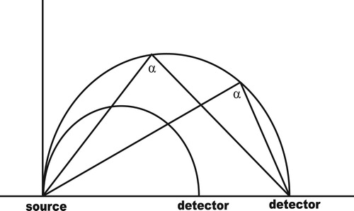
When monoenergetic x-rays or gamma-rays are emitted isotropically into a plane, singly-Compton scattered photons that suffer the same energy loss will lie on a circular arc. This arc will pass though the source and detector location and its radius will be defined by the photon energy. When multiple measurements are made by varying the source and/or detector locations with energy-sensitive detection, an image can be reconstructed from the path integrals of electron density measured over these multiple overlapping circular arcs. This tomography problem based on Compton-scattered photons was originally examined by the author [1] under the assumption of a single fixed source location and multiple detector locations along a line, as illustrated in Figure 1.

Figure 1. In this configuration, there is one source and a linear array of energy-sensitive detectors. The scattering angle α is the same for all points on the larger arc shown. This implies the same Compton-scattering energy loss for all points on this arc.

A solution in the form of a filtered-backprojection approach was derived in that article for the geometry shown in Figure 1. It has since been noted that sufficient data can be acquired for a reconstruction using one source and one detector if the object is rotated between the source and detector or, equivalently, if the source and detector are rotated about the object [2–4]. In this rotating geometry, we show that a simple transformation of variables allows us to express the curved path-integral reconstruction problem in a form identical to that of the filtered-backprojection solution to the straight path-integral problem. The above published approaches to the Compton tomography reconstruction problem in the rotating geometry are based a solution derived by Cormack that employs a circular harmonic expansion of the data and image [5]. Cormack's method, however, requires some form of regularization because the inversion of the higher-order harmonics is ill-conditioned. Cormack's solution also contains a derivative of the measured path integrals and a singularity in the kernel, which can be problematic with noisy data. On the other hand, the filtered-backprojection method is well conditioned since the tomographic filter effectively performs the function of regularization and avoids differentiating the path-integral data. A similar filtered-backprojection formula was derived in [2] using a less direct route derived from the circular-harmonic inverse Radon transform. Most of the above publications on Compton tomography neglect attenuation for the sake of mathematical tractability. The problem of accounting for attenuation is discussed in the conclusion. As noted, the locus of points over which the Compton scattered photons suffer the same energy loss is a circular arc subtending the same scattering angle α, where the relation between α and the photon energy is given by (1) $E_{\alpha }=\frac{E_0}{1+\kappa (1+\cos \alpha )}.$(1) Here $\kappa =E_0/m_e{c}^2$, $E_0$ is the energy of the incident photon and $m_e{c}^2$ is the rest energy of the electron.

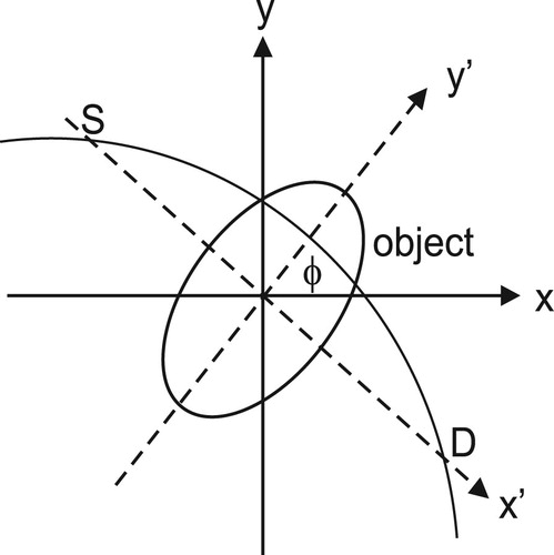
Let us denote the unknown object by the function $f(x,y)$ which, as shown below, will be related to the electron density. We assume that the source and detector lie on the $x^{\prime }$-axis of a rotated coordinate system $(x^{\prime },y^{\prime })$, as shown in Figure 2, where the rotation angle φ is shown in the figure. 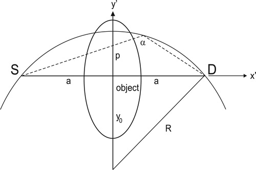From the figure (2) $\begin{array}{rl}{x}^{\prime }& =x\sin \varphi -y\cos \varphi \\ y^{\prime }& =x\cos \varphi +y\sin \varphi \end{array}$(2) As shown in Figure 3, the circular arc passes through the source and detector on the $x^{\prime }$-axis separated by the distance $2a$ and the arc's radius is defined by the scattering angle α. One can show from the geometry that the radius R of the arc is related to the scattering angle α by $R=a/\sin \alpha$, and the centre of the arc is located on the negative $y^{\prime }$-axis at a distance $y_0=-a\cot \alpha$. Any point $(x^{\prime },y^{\prime })$ on the arc obeys $x^{\prime 2}+(y^{\prime }+y_0{)}^2=R^2$, where $R^2=a^2+y_0^2$.

Figure 2. The source and detector lie on the $x^{\prime }$-axis of the rotated coordinate system.

Now suppose the function f is defined over a domain between the points $(-a,0)$ and $(a,0)$. We shall assume that $f(x,y)\equiv 0$ outside a circle of radius a. We rotate the source-detector though the angle φ and record measurements of the function $f(x,y)$ over the range of rotation angles $0\le \varphi \le 2\pi$, where our independent variables are ($y_0$,φ). We shall further assume that the source generates a 2-D fan beam that illuminates the object in the upper half of the $x^{\prime }$-$y^{\prime }$ plane ($y^{\prime }\ge 0$) by suitably designed collimators. In this case, the locus of scattering points below the $x^{\prime }$-axis is excluded. Then our fundamental equation from which we wish to reconstruct $f(r,\theta )$ is the path integral defined by (3) $g(y_0,\varphi )={\int }_{-\mathrm{\infty }}^{\mathrm{\infty }}{\int }_{-\mathrm{\infty }}^{\mathrm{\infty }}\mathrm{d}x\mathrm{d}yf(x,y)\delta (R-\sqrt{x^{\prime 2}+(y^{\prime }+y_0{)}^2}).$(3) Converting to polar coordinates using $x=r\cos \theta$ and $y=r\sin \theta$ and transforming from $(x^{\prime },y^{\prime })$ to $(x,y)$ inside the δ function using the transformation (2(2) $\begin{array}{rl}{x}^{\prime }& =x\sin \varphi -y\cos \varphi \\ y^{\prime }& =x\cos \varphi +y\sin \varphi \end{array}$(2) ), (3(3) $g(y_0,\varphi )={\int }_{-\mathrm{\infty }}^{\mathrm{\infty }}{\int }_{-\mathrm{\infty }}^{\mathrm{\infty }}\mathrm{d}x\mathrm{d}yf(x,y)\delta (R-\sqrt{x^{\prime 2}+(y^{\prime }+y_0{)}^2}).$(3) ) becomes (4) $g(y_0,\varphi )={\int }_0^{\mathrm{\infty }}r\mathrm{d}r{\int }_0^{2\pi }\mathrm{d}\theta f(r,\theta )\delta (R-\sqrt{r^2+2y_{0}r\cos (\varphi -\theta )+y_0^2}).$(4)

Figure 3. The centre of the arc lies a distance $y_0$ below the $x^{\prime }$-axis and the arc passes through the source (S) and detector (D).

Our objective is to show how we can solve this integral equation for $f(r,\theta )$ in terms of $g(y_0,\varphi )$. We note here that the path-integral data $g(y_0,\varphi )$ can be weighted by any function that depends on the scattering angle α, which in turn is related to the variable $y_0$. Such a function is the Klein-Nishina differential scattering cross-section for Compton scattering [6]. To be more explicit, (4(4) $g(y_0,\varphi )={\int }_0^{\mathrm{\infty }}r\mathrm{d}r{\int }_0^{2\pi }\mathrm{d}\theta f(r,\theta )\delta (R-\sqrt{r^2+2y_{0}r\cos (\varphi -\theta )+y_0^2}).$(4) ) should be written as a weighted path integral of the form (5) $\overline{g}(y_0,\varphi )={\int }_0^{\mathrm{\infty }}r\mathrm{d}r{\int }_0^{2\pi }\mathrm{d}\theta w(y_0,\varphi ;r,\theta )\overline{f}(r,\theta )\delta (R-\sqrt{r^2+2y_{0}r\cos (\varphi -\theta )+y_0^2}).$(5)

In the absence of attenuation, the weight w factors as $w(y_0,\varphi ;r,\theta )=w_1(y_0,\varphi )w_2(r,\theta )$, where $w_1(y_0,\varphi )$ contains the Klein-Nishina cross-section. The function $w_2(r,\theta )$ can incorporate the variation of the solid angles subtended by the source and detector and a possible angular variation of the source. Our treatment here neglects photon absorption from the source to the scattering location and to the detector. An approximate treatment of attenuation is given in [1] that still permits the factorization of w. For brevity, we shall use (4(4) $g(y_0,\varphi )={\int }_0^{\mathrm{\infty }}r\mathrm{d}r{\int }_0^{2\pi }\mathrm{d}\theta f(r,\theta )\delta (R-\sqrt{r^2+2y_{0}r\cos (\varphi -\theta )+y_0^2}).$(4) ) and assume that $w_1(y_0,\varphi )$ and $w_2(r,\theta )$ are absorbed into the definitions of $g(y_0,\varphi )$ and $f(r,\theta )$, respectively, by defining $g=\overline{g}/w_1$ and $f=\overline{f}{w}_2$.

Before inverting (4(4) $g(y_0,\varphi )={\int }_0^{\mathrm{\infty }}r\mathrm{d}r{\int }_0^{2\pi }\mathrm{d}\theta f(r,\theta )\delta (R-\sqrt{r^2+2y_{0}r\cos (\varphi -\theta )+y_0^2}).$(4) ) for $f(r,\theta )$, we briefly review the derivation of the filtered-backprojection formula for the conventional CT problem in which the path integrals are measured over straight lines. This is useful since we will transform our problem into a form identical to the straight path problem and then employ the same solution method.

2. Reconstruction from line integrals over straight paths

Here the path integral, $g(p,\varphi )$, is defined along the straight line parameterized by $(p,\varphi )$, where p is the perpendicular distance from the line to the origin and φ is the angle that this perpedicular makes with the x axis; that is, in polar form (6) $g(p,\varphi )={\int }_0^{\mathrm{\infty }}r\mathrm{d}r{\int }_0^{2\pi }\mathrm{d}\theta f(r,\theta )\delta [p-r\cos (\varphi -\theta )],$(6) which can be written (7) $g(p,\varphi )={\int }_0^{\mathrm{\infty }}r\mathrm{d}r{\int }_0^{2\pi }\mathrm{d}\theta f(r,\theta )\frac{1}{2\pi }{\int }_{-\mathrm{\infty }}^{\mathrm{\infty }}\mathrm{d}k{e}^{ikp}{e}^{-ikr\cos (\varphi -\theta )}.$(7)

Here we have assumed that $-\mathrm{\infty }<p<\mathrm{\infty }$ and $0\le \varphi \le \pi$. However, it may be more convenient to assume $p\ge 0$, in which case we let $0\le \varphi <2\pi$. This can be achieved using the relation $g(-p,\varphi )=g(p,\varphi +\pi )$. Now the Fourier transform of the path integral $g(p,\varphi )$ with respect to p is (8) $\tilde{g}(k,\varphi )={\int }_{-\mathrm{\infty }}^{\mathrm{\infty }}g(p,\varphi )e^{-ikp}\mathrm{d}p.$(8)

Substituting (7(7) $g(p,\varphi )={\int }_0^{\mathrm{\infty }}r\mathrm{d}r{\int }_0^{2\pi }\mathrm{d}\theta f(r,\theta )\frac{1}{2\pi }{\int }_{-\mathrm{\infty }}^{\mathrm{\infty }}\mathrm{d}k{e}^{ikp}{e}^{-ikr\cos (\varphi -\theta )}.$(7) ) into (8(8) $\tilde{g}(k,\varphi )={\int }_{-\mathrm{\infty }}^{\mathrm{\infty }}g(p,\varphi )e^{-ikp}\mathrm{d}p.$(8) ) and performing the p integration results in (9) $\begin{array}{rl}\tilde{g}(k,\varphi )& ={\int }_0^{\mathrm{\infty }}r\mathrm{d}r{\int }_0^{2\pi }\mathrm{d}\theta f(r,\theta )e^{-ikr\cos (\varphi -\theta )}\\ & ={\mathcal{F}}_{2D}\{f(r,\theta ){\}}_{k,\varphi }.\end{array}$(9)

This is the 2-D Fourier transform of $f(r,\theta )$ in polar coordinates. The 2-D inverse Fourier transform then gives (10) $\begin{array}{rl}f(r,\theta )& =\frac{1}{(2\pi {)}^2}{\int }_0^{2\pi }\mathrm{d}\varphi {\int }_0^{\mathrm{\infty }}k\mathrm{d}k\tilde{g}(k,\varphi )e^{ikr\cos (\varphi -\theta )}\\ & =\frac{1}{(2\pi {)}^2}{\int }_0^{\pi }\mathrm{d}\varphi {\int }_{-\mathrm{\infty }}^{\mathrm{\infty }}|k|\mathrm{d}k\tilde{g}(k,\varphi )e^{ikr\cos (\varphi -\theta )},\end{array}$(10) where in the last step we have employed the relation $\tilde{g}(-k,\varphi )=\tilde{g}(k,\varphi +\pi )$. Now define the filtered path integral $g_f(p,\varphi )$: (11) $g_f(p,\varphi )=\frac{1}{2\pi }{\int }_{-\mathrm{\infty }}^{\mathrm{\infty }}|k|\tilde{g}(k,\varphi )e^{ikp}\mathrm{d}k.$(11)

Comparing (10(10) $\begin{array}{rl}f(r,\theta )& =\frac{1}{(2\pi {)}^2}{\int }_0^{2\pi }\mathrm{d}\varphi {\int }_0^{\mathrm{\infty }}k\mathrm{d}k\tilde{g}(k,\varphi )e^{ikr\cos (\varphi -\theta )}\\ & =\frac{1}{(2\pi {)}^2}{\int }_0^{\pi }\mathrm{d}\varphi {\int }_{-\mathrm{\infty }}^{\mathrm{\infty }}|k|\mathrm{d}k\tilde{g}(k,\varphi )e^{ikr\cos (\varphi -\theta )},\end{array}$(10) ) and (11(11) $g_f(p,\varphi )=\frac{1}{2\pi }{\int }_{-\mathrm{\infty }}^{\mathrm{\infty }}|k|\tilde{g}(k,\varphi )e^{ikp}\mathrm{d}k.$(11) ) shows that the reconstruction can be written as an angular integration over the backprojected filtered path integrals: (12) $f(r,\theta )=\frac{1}{2\pi }{\int }_0^{\pi }{g}_f[r\cos (\varphi -\theta ),\varphi ]\mathrm{d}\varphi ,$(12) or in rectangular coordinates, (13) $f(x,y)=\frac{1}{2\pi }{\int }_0^{\pi }{g}_f[x\cos \varphi +y\sin \varphi ,\varphi ]\mathrm{d}\varphi .$(13)

The latter is a standard form of the filtered-backprojection solution to the CT reconstruction problem.

3. Reconstruction from line integrals over curved paths

We now return to the problem of reconstructing the object function $f(r,\theta )$ from (4(4) $g(y_0,\varphi )={\int }_0^{\mathrm{\infty }}r\mathrm{d}r{\int }_0^{2\pi }\mathrm{d}\theta f(r,\theta )\delta (R-\sqrt{r^2+2y_{0}r\cos (\varphi -\theta )+y_0^2}).$(4) ). We can rewrite this equation using the following properties of the delta function: $\delta (R-\sqrt{X})=2R\delta (R^2-X)$ when R>0, and $\delta (rX)=\delta (X)/r$ for $r>0$. We then have (14) $\begin{array}{rl}g(y_0,\varphi )& =2R{\int }_0^{\mathrm{\infty }}r\mathrm{d}r{\int }_0^{2\pi }\mathrm{d}\theta f(r,\theta )\delta (R^2-r^2-2y_{0}r\cos (\varphi -\theta )-y_0^2)\\ & =2R{\int }_0^{\mathrm{\infty }}r\mathrm{d}r{\int }_0^{2\pi }\mathrm{d}\theta f(r,\theta )\delta [a^2-r^2-2y_{0}r\cos (\varphi -\theta )]\\ & =2R{\int }_0^{\mathrm{\infty }}\mathrm{d}r{\int }_0^{2\pi }\mathrm{d}\theta f(r,\theta )\delta [(a^2-r^2)/r-2y_0\cos (\varphi -\theta )],\end{array}$(14) where in the second line we used $R^2=y_0^2+a^2$. Now note from the geometry of Figure 3 that $p=R-y_0=\sqrt{y_0^2+a^2}-y_0$. Solving for $y_0$ in terms of p, we obtain $2y_0=(a^2-p^2)/p$. Now define the function (15) $s(x)\equiv \frac{x}{1-(x/a{)}^2}.$(15)

Then the delta function in (14(14) $\begin{array}{rl}g(y_0,\varphi )& =2R{\int }_0^{\mathrm{\infty }}r\mathrm{d}r{\int }_0^{2\pi }\mathrm{d}\theta f(r,\theta )\delta (R^2-r^2-2y_{0}r\cos (\varphi -\theta )-y_0^2)\\ & =2R{\int }_0^{\mathrm{\infty }}r\mathrm{d}r{\int }_0^{2\pi }\mathrm{d}\theta f(r,\theta )\delta [a^2-r^2-2y_{0}r\cos (\varphi -\theta )]\\ & =2R{\int }_0^{\mathrm{\infty }}\mathrm{d}r{\int }_0^{2\pi }\mathrm{d}\theta f(r,\theta )\delta [(a^2-r^2)/r-2y_0\cos (\varphi -\theta )],\end{array}$(14) ) may be written (16) $\begin{array}{rl}\delta [(a^2-r^2)/r-2y_0\cos (\varphi -\theta )]& =\delta \{\frac{a^2}{s(r)}-\frac{a^2}{s(p)}\cos (\varphi -\theta )\}\\ & =\frac{s(r)s(p)}{a^2}\delta \{s(p)-s(r)\cos (\varphi -\theta )\},\end{array}$(16) which holds when $s(r)>0$ and $s(p)>0$. In view of (15(15) $s(x)\equiv \frac{x}{1-(x/a{)}^2}.$(15) ), both $s(r)$ and $s(p)$ are positive when r and p are both less than a, which we assume. Then (14(14) $\begin{array}{rl}g(y_0,\varphi )& =2R{\int }_0^{\mathrm{\infty }}r\mathrm{d}r{\int }_0^{2\pi }\mathrm{d}\theta f(r,\theta )\delta (R^2-r^2-2y_{0}r\cos (\varphi -\theta )-y_0^2)\\ & =2R{\int }_0^{\mathrm{\infty }}r\mathrm{d}r{\int }_0^{2\pi }\mathrm{d}\theta f(r,\theta )\delta [a^2-r^2-2y_{0}r\cos (\varphi -\theta )]\\ & =2R{\int }_0^{\mathrm{\infty }}\mathrm{d}r{\int }_0^{2\pi }\mathrm{d}\theta f(r,\theta )\delta [(a^2-r^2)/r-2y_0\cos (\varphi -\theta )],\end{array}$(14) ) becomes (17) $g(y_0,\varphi )=\frac{2Rs(p)}{a^2}{\int }_0^{\mathrm{\infty }}\mathrm{d}r{\int }_0^{2\pi }\mathrm{d}\theta f(r,\theta )s(r)\delta \{s(p)-s(r)\cos (\varphi -\theta )\}.$(17) From the relation $2y_0=a^2/s(p)$, we can transform between $y_0$ and the new variable $s(p)$. We now define (18) $G[s(p),\varphi ]\equiv \frac{a^{2}g(y_0,\varphi )}{2Rs(p)},$(18) so that (17(17) $g(y_0,\varphi )=\frac{2Rs(p)}{a^2}{\int }_0^{\mathrm{\infty }}\mathrm{d}r{\int }_0^{2\pi }\mathrm{d}\theta f(r,\theta )s(r)\delta \{s(p)-s(r)\cos (\varphi -\theta )\}.$(17) ) becomes (19) $G[s(p),\varphi ]={\int }_0^{\mathrm{\infty }}\mathrm{d}r{\int }_0^{2\pi }\mathrm{d}\theta f(r,\theta )s(r)\delta \{s(p)-s(r)\cos (\varphi -\theta )\}.$(19)

We can express this equation in a form identical to the straight-path formula by defining (20) $F[s(r),\theta ]\equiv \frac{f(r,\theta )}{s^{\prime }(r)},$(20) where $s^{\prime }(r)$ is the derivative of $s(r)$ which, from (15(15) $s(x)\equiv \frac{x}{1-(x/a{)}^2}.$(15) ) is given by $s^{\prime }(r)=a^2(a^2+r^2)/(a^2-r^2{)}^2$. Then noting that $\mathrm{d}s(r)=s^{\prime }(r)\mathrm{d}r$ and writing for brevity $s_p=s(p)$ and $s_r=s(r)$, (19(19) $G[s(p),\varphi ]={\int }_0^{\mathrm{\infty }}\mathrm{d}r{\int }_0^{2\pi }\mathrm{d}\theta f(r,\theta )s(r)\delta \{s(p)-s(r)\cos (\varphi -\theta )\}.$(19) ) may be written (21) $G(s_p,\varphi )={\int }_0^{\mathrm{\infty }}{s}_r\mathrm{d}{s}_r{\int }_0^{2\pi }\mathrm{d}\theta F(s_r,\theta )\delta [s_p-s_r\cos (\varphi -\theta )],$(21) which is now in a form identical to that of (6(6) $g(p,\varphi )={\int }_0^{\mathrm{\infty }}r\mathrm{d}r{\int }_0^{2\pi }\mathrm{d}\theta f(r,\theta )\delta [p-r\cos (\varphi -\theta )],$(6) ). Thus G and F play the role of f and g in the standard straight-path problem. We can invert this in a similar fashion. First write (22) $G(s_p,\varphi )=\frac{1}{2\pi }{\int }_0^{\mathrm{\infty }}{s}_r\mathrm{d}{s}_r{\int }_0^{2\pi }\mathrm{d}\theta F(s_r,\theta ){\int }_{-\mathrm{\infty }}^{\mathrm{\infty }}\mathrm{d}k{e}^{ik[s_p-s_r\cos (\varphi -\theta )]}.$(22)

We now wish to Fourier transform this equation with respect to the variable $s_p$. Thus far, we have assumed $s_p\ge 0$ with $0\le \varphi <2\pi$. However, in performing the Fourier transform, we can extend the range of $s_p$ to negative values using the relation $G(s_p,\varphi )=G(-s_p,\varphi +\pi )$ with $0\le \varphi \le \pi$. The Fourier transform then becomes (23) $\begin{array}{rl}\tilde{G}(k,\varphi )& \equiv {\int }_{-\mathrm{\infty }}^{\mathrm{\infty }}G(s_p,\varphi )e^{-ik{s}_p}\mathrm{d}{s}_p\\ & ={\int }_0^{\mathrm{\infty }}{s}_r\mathrm{d}{s}_r{\int }_0^{2\pi }\mathrm{d}\theta F(s_r,\theta )e^{-ik{s}_r\cos (\varphi -\theta )},\end{array}$(23) which is the 2-D Fourier transform of $F(s_r,\theta )$ in polar form. Inverse Fourier transforming results in (24) $F(s_r,\theta )=\frac{1}{(2\pi {)}^2}{\int }_0^{2\pi }\mathrm{d}\varphi {\int }_0^{\mathrm{\infty }}k\mathrm{d}k\tilde{G}(k,\varphi )e^{ik{s}_r\cos (\varphi -\theta )}.$(24)

Or from (20(20) $F[s(r),\theta ]\equiv \frac{f(r,\theta )}{s^{\prime }(r)},$(20) ), (25) $f(r,\theta )=\frac{s^{\prime }(r)}{(2\pi {)}^2}{\int }_0^{\pi }\mathrm{d}\varphi {\int }_{-\mathrm{\infty }}^{\mathrm{\infty }}|k|\mathrm{d}k\tilde{G}(k,\varphi )e^{ik{s}_r\cos (\varphi -\theta )}.$(25)

Now define the filtered $G(s_p,\varphi )$ by (26) $G_f(t,\varphi )\equiv {\int }_{-\mathrm{\infty }}^{\mathrm{\infty }}\tilde{G}(k,\varphi )e^{ikt}|k|\mathrm{d}k.$(26)

Then (25(25) $f(r,\theta )=\frac{s^{\prime }(r)}{(2\pi {)}^2}{\int }_0^{\pi }\mathrm{d}\varphi {\int }_{-\mathrm{\infty }}^{\mathrm{\infty }}|k|\mathrm{d}k\tilde{G}(k,\varphi )e^{ik{s}_r\cos (\varphi -\theta )}.$(25) ) may be written in the backprojection from: (27) $f(r,\theta )=\frac{s^{\prime }(r)}{(2\pi {)}^2}{\int }_0^{\pi }{G}_f[s_r\cos (\varphi -\theta ),\varphi ]\mathrm{d}\varphi .$(27)

Note that we can write (28) $\begin{array}{rl}{s}_r\cos (\varphi -\theta )& =s_r\cos \theta \cos \varphi +s_r\sin \theta \sin \varphi \\ & =\frac{r\cos \theta }{1-(r/a{)}^2}\cos \varphi +\frac{r\sin \theta }{1-(r/a{)}^2}\sin \varphi \\ & =\frac{x\cos \varphi +y\sin \varphi }{1-r^2/a^2}.\end{array}$(28)

Or in rectangular coordinates, (29) $f(x,y)=\frac{s^{\prime }(r)}{(2\pi {)}^2}{\int }_0^{\pi }{G}_f\left[\frac{x\cos \varphi +y\sin \varphi }{1-r^2/a^2}\right]\mathrm{d}\varphi ,$(29) where $r^2=x^2+y^2$ and $s^{\prime }(r)=a^2(a^2+r^2)/(a^2-r^2{)}^2$. This is the desired result: the filtered-backprojection solution for curved paths.

As a check, when $r\ll a\ll y_0$, the curves intersecting the domain of $f(r,\theta )$ become approximately straight and the formulas (27(27) $f(r,\theta )=\frac{s^{\prime }(r)}{(2\pi {)}^2}{\int }_0^{\pi }{G}_f[s_r\cos (\varphi -\theta ),\varphi ]\mathrm{d}\varphi .$(27) ) or (29(29) $f(x,y)=\frac{s^{\prime }(r)}{(2\pi {)}^2}{\int }_0^{\pi }{G}_f\left[\frac{x\cos \varphi +y\sin \varphi }{1-r^2/a^2}\right]\mathrm{d}\varphi ,$(29) ) should reduce to the standard (CT) straight-line backprojection formula (13(13) $f(x,y)=\frac{1}{2\pi }{\int }_0^{\pi }{g}_f[x\cos \varphi +y\sin \varphi ,\varphi ]\mathrm{d}\varphi .$(13) ) in this limit. To show this, note that when $r\ll a$, we have $s(r)\approx r$, $s^{\prime }(r)\approx 1$ and $s(p)\approx p$, so that (29(29) $f(x,y)=\frac{s^{\prime }(r)}{(2\pi {)}^2}{\int }_0^{\pi }{G}_f\left[\frac{x\cos \varphi +y\sin \varphi }{1-r^2/a^2}\right]\mathrm{d}\varphi ,$(29) ) reduces to (30) $f(x,y)=\frac{1}{(2\pi {)}^2}{\int }_0^{\pi }{G}_f[x\cos \varphi +y\sin \varphi ,\varphi ]\mathrm{d}\varphi .$(30)

It is also readily shown that in this limit $G\to g$ and, as a consequence, $G_f\to g_f$, as required.

When the transformed path integral $G(s_p,\varphi )$ is filtered according to (26(26) $G_f(t,\varphi )\equiv {\int }_{-\mathrm{\infty }}^{\mathrm{\infty }}\tilde{G}(k,\varphi )e^{ikt}|k|\mathrm{d}k.$(26) ), practical algorithms typically replace $|k|$ with a filter $A(k)$ that proceeds smoothly to some spatial frequency cutoff $k_m$, but behaves like $|k|$ at lower spatial frequencies. That is, (26(26) $G_f(t,\varphi )\equiv {\int }_{-\mathrm{\infty }}^{\mathrm{\infty }}\tilde{G}(k,\varphi )e^{ikt}|k|\mathrm{d}k.$(26) ) might be replaced by (31) ${\hat{G}}_f(t,\varphi )\equiv {\int }_{-\mathrm{\infty }}^{\mathrm{\infty }}\tilde{G}(k,\varphi )e^{-ikt}A(k)\mathrm{d}k.$(31)

An example of such a filter is $A(k)=k_m|\sin (\pi k/k_m)|/\pi$ and $A(k)=0$ for $k>k_m$. The latter form is used in our example described in the next section.

4. Example

As a simple example to check the solution, we consider the following axi-symmetric object. Let (32) $f(r,\theta )\equiv f(r)=\{\begin{array}{ll}1,& r_1\le r\le r_2\\ 0& \text{otherwise.}\end{array}$(32)

Because of angular symmetry, we write $g(y_0,\varphi )=g(y_0)$. This example is simple enough so that we can write down the path integral $g(y_0)$ explicitly. First consider the simpler case of $f(r)=$ circ($r/r_2$) = 1 for $0\le r\le r_2$ and zero otherwise. In the latter case, from Figure 4, $g(y_0)$ is just the length of the arc with centre at a distance $y_0$ below the origin of radius $R=\sqrt{y_0^2+a^2}$ that intersects the region circ($r/r_2$). This arc is defined by the parameters a and $y_0$.

Figure 4. The path integral through circ($r/r_2$) is the length of the arc that intersects the dashed circle.

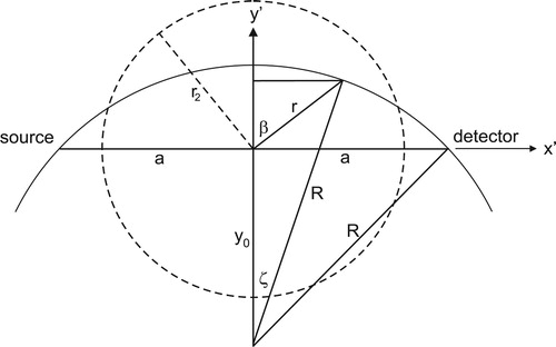
We see from the figure that the relation between the radius r from the origin to a point on the arc and the angles ζ and β is given by: $\begin{array}{rl}r\sin \beta & =R\sin \zeta \\ r\cos \beta +y_0& =R\cos \zeta \end{array}$

Eliminating β yields (33) $\cos \zeta =\frac{R^2+y_0^2-r^2}{2R{y}_0},$(33) or (34) $\zeta ={\cos }^{-1}\left(\frac{R^2+y_0^2-r^2}{2R{y}_0}\right).$(34)

Now the length of the arc that intersects circ($r/r_2$) at radius r is given by (35) $g(y_0)=2R{\zeta }_2,$(35) where (36) ${\zeta }_2={\cos }^{-1}\left(\frac{R^2+y_0^2-r_2^2}{2R{y}_0}\right).$(36)

Then the length of the arc that intersects the annular region defined by (32(32) $f(r,\theta )\equiv f(r)=\{\begin{array}{ll}1,& r_1\le r\le r_2\\ 0& \text{otherwise.}\end{array}$(32) ) is just (37) $g(y_0)=2R({\zeta }_2-{\zeta }_1),$(37) where (38) ${\zeta }_1={\cos }^{-1}\left(\frac{R^2+y_0^2-r_1^2}{2R{y}_0}\right).$(38)

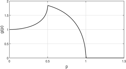
The path-integral function $g(y_0)$ defined by (37(37) $g(y_0)=2R({\zeta }_2-{\zeta }_1),$(37) ) when $r_1=0.5$ and $r_2=1$ is plotted in Figure 5 versus p, where $p\equiv \sqrt{a^2+y_0^2}-y_0$.

Figure 5. The path integral g versus p.

Recalling the path-integral change of variables $G=a^{2}g/(2R{s}_p)$, we have (39) $G(s_p)=\frac{a^2}{s_p}({\zeta }_2-{\zeta }_1)=\frac{a^2}{s_p}[{\cos }^{-1}(q_2)-{\cos }^{-1}(q_1)],$(39) where the arguments of the ${\cos }^{-1}$ are given by (40) $\begin{array}{rl}{q}_1& =\frac{2y_0^2+a^2-r_1^2}{2y_0\sqrt{y_0^2+a^2}}=\frac{a^4+2(a^2-r_1^2)s_p^2}{a^3\sqrt{a^2+4s_p^2}}\end{array}$(40) (41) $\begin{array}{rl}{q}_2& =\frac{2y_0^2+a^2-r_2^2}{2y_0\sqrt{y_0^2+a^2}}=\frac{a^4+2(a^2-r_2^2)s_p^2}{a^3\sqrt{a^2+4s_p^2}}.\end{array}$(41)

In the left-hand expressions, we have converted from $y_0$ to $s_p$ using the relation $2y_0=a^2/s_p$.

To solve this problem, it is convenient to start with (25(25) $f(r,\theta )=\frac{s^{\prime }(r)}{(2\pi {)}^2}{\int }_0^{\pi }\mathrm{d}\varphi {\int }_{-\mathrm{\infty }}^{\mathrm{\infty }}|k|\mathrm{d}k\tilde{G}(k,\varphi )e^{ik{s}_r\cos (\varphi -\theta )}.$(25) ): (42) $f(r)=\frac{s^{\prime }(r)}{(2\pi {)}^2}{\int }_0^{\pi }\mathrm{d}\varphi {\int }_{-\mathrm{\infty }}^{\mathrm{\infty }}\mathrm{d}kA(k)\tilde{G}(k)e^{ik{s}_r\cos \varphi },$(42) where, because of symmetry, we have written $f(r,\theta )=f(r)$ and $\tilde{G}(k,\varphi )=\tilde{G}(k)$. In (42(42) $f(r)=\frac{s^{\prime }(r)}{(2\pi {)}^2}{\int }_0^{\pi }\mathrm{d}\varphi {\int }_{-\mathrm{\infty }}^{\mathrm{\infty }}\mathrm{d}kA(k)\tilde{G}(k)e^{ik{s}_r\cos \varphi },$(42) ) we have also replaced $|k|$ with the filter function $A(k)=k_m|\sin (\pi k/k_m)|/\pi$ and $A(k)=0$ for $k>k_m$, which goes smoothly to zero at the cutoff $k_m$. Because $\tilde{G}(k)$ is independent of φ, so is $G(s_p)$. As a result, the Fourier transform given by the first line of (23(23) $\begin{array}{rl}\tilde{G}(k,\varphi )& \equiv {\int }_{-\mathrm{\infty }}^{\mathrm{\infty }}G(s_p,\varphi )e^{-ik{s}_p}\mathrm{d}{s}_p\\ & ={\int }_0^{\mathrm{\infty }}{s}_r\mathrm{d}{s}_r{\int }_0^{2\pi }\mathrm{d}\theta F(s_r,\theta )e^{-ik{s}_r\cos (\varphi -\theta )},\end{array}$(23) ), may be written (43) $\tilde{G}(k)=2{\int }_0^{\mathrm{\infty }}G(s_p)\cos (k{s}_p)\mathrm{d}{s}_p.$(43)

Inserting this into (42(42) $f(r)=\frac{s^{\prime }(r)}{(2\pi {)}^2}{\int }_0^{\pi }\mathrm{d}\varphi {\int }_{-\mathrm{\infty }}^{\mathrm{\infty }}\mathrm{d}kA(k)\tilde{G}(k)e^{ik{s}_r\cos \varphi },$(42) ), interchanging orders of integration and performing the φ integral gives (44) $f(r)=\frac{s^{\prime }(r)}{\pi }{\int }_0^{\mathrm{\infty }}\mathrm{d}{s}_{p}G(s_p){\int }_0^{\mathrm{\infty }}\mathrm{d}kA(k)J_0(k{s}_r)\cos (k{s}_p),$(44) where $J_0$ is the zero-order Bessel function of the first kind. If we set $A(k)=|k|$, we can show analytically that this equation recovers (32(32) $f(r,\theta )\equiv f(r)=\{\begin{array}{ll}1,& r_1\le r\le r_2\\ 0& \text{otherwise.}\end{array}$(32) ) after inserting $G(s_p)$ given by (39(39) $G(s_p)=\frac{a^2}{s_p}({\zeta }_2-{\zeta }_1)=\frac{a^2}{s_p}[{\cos }^{-1}(q_2)-{\cos }^{-1}(q_1)],$(39) ). This is most easily demonstrated by first integrating (44(44) $f(r)=\frac{s^{\prime }(r)}{\pi }{\int }_0^{\mathrm{\infty }}\mathrm{d}{s}_{p}G(s_p){\int }_0^{\mathrm{\infty }}\mathrm{d}kA(k)J_0(k{s}_r)\cos (k{s}_p),$(44) ) by parts giving (45) $\begin{array}{rl}f(r)& =-\frac{s^{\prime }(r)}{\pi }{\int }_0^{\mathrm{\infty }}\mathrm{d}{s}_p{G}^{\prime }(s_p){\int }_0^{\mathrm{\infty }}\mathrm{d}k{J}_0(k{s}_r)\sin (k{s}_p)\\ & =-\frac{s^{\prime }(r)}{\pi }{\int }_{s_r}^{\mathrm{\infty }}\mathrm{d}{s}_p\frac{G^{\prime }(s_p)\mathrm{d}{s}_p}{\sqrt{s_p^2-s_r^2}},\end{array}$(45) where $G^{\prime }(s_p)$ is the derivative of $G(s_p)$. Note that the integral is just the inverse Abel transform of $G(s_p)$ in the new variable $s_p$. After differentiating $G(s_p)$ as given by (39(39) $G(s_p)=\frac{a^2}{s_p}({\zeta }_2-{\zeta }_1)=\frac{a^2}{s_p}[{\cos }^{-1}(q_2)-{\cos }^{-1}(q_1)],$(39) ), inserting the result into (45(45) $\begin{array}{rl}f(r)& =-\frac{s^{\prime }(r)}{\pi }{\int }_0^{\mathrm{\infty }}\mathrm{d}{s}_p{G}^{\prime }(s_p){\int }_0^{\mathrm{\infty }}\mathrm{d}k{J}_0(k{s}_r)\sin (k{s}_p)\\ & =-\frac{s^{\prime }(r)}{\pi }{\int }_{s_r}^{\mathrm{\infty }}\mathrm{d}{s}_p\frac{G^{\prime }(s_p)\mathrm{d}{s}_p}{\sqrt{s_p^2-s_r^2}},\end{array}$(45) ) and performing the integral, we recover (32(32) $f(r,\theta )\equiv f(r)=\{\begin{array}{ll}1,& r_1\le r\le r_2\\ 0& \text{otherwise.}\end{array}$(32) ). 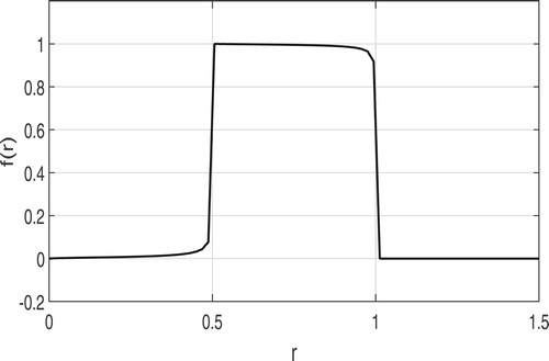For a numerical inversion, we keep the filter $A(k)$ in (42(42) $f(r)=\frac{s^{\prime }(r)}{(2\pi {)}^2}{\int }_0^{\pi }\mathrm{d}\varphi {\int }_{-\mathrm{\infty }}^{\mathrm{\infty }}\mathrm{d}kA(k)\tilde{G}(k)e^{ik{s}_r\cos \varphi },$(42) ), insert the modified path integral $G(s_p)$ and perform the k and $s_p$ integrals numerically. This results in the reconstruction shown in Figure 6.

Figure 6. Profile of the reconstructed function $f(r)$.

5. Discussion and conclusion

Much has been written about Compton scattering tomography in the last two decades, although its utility as a practical modality for medical diagnostic imaging is still uncertain. An advantage of the Compton scattering approach that is frequently noted is the higher contrast of scattering-based images compared to transmission CT images, which would be helpful in imaging, for example, calcifications in the breast. However, the reconstruction problem described here and in many other publications is highly idealized: we neglect attenuation, neglect contamination due to multiple scattering (assume only singly-scattered photons) and have assumed idealized detectors with perfect energy resolution. These assumptions permit a tractable mathematical analysis. One could argue that the idealized problem does provide insight into the reconstruction problem in the same way that the inverse Radon transform does as the idealized solution to the x-ray CT problem. Studies of some of the practical aspects of real systems have been made [7–10]. Norton [1] proposed a semi-analytical treatment of attenuation (which arises primarily from photo-electric absorption and higher-order scattering), but only when the attenuation is approximated as homogeneous in the scattering medium. For nonuniform attenuation, an iterative approach was suggested. Monte-Carlo simulations that take into account both multiple scattering and photoelectric absorption would be very useful.

As noted, the rotational geometry with a single source and detector as discussed in this paper and in other publications has the advantage of allowing a mathematical solution. A practical drawback of such a system is the inefficiency of a single detector, which increases the recording time and thus the radiation dose. One way to improve efficiency is to use multiple detectors. Unfortunately, the generalization of the filtered-backprojection solution described here to multiple detectors is not possible because the analysis requires that the location of the centre of rotation lie on the line joining the source and detector, and this requirement will not hold for all elements in a detector array. An alternative that avoids this requirement is to use a purely numerical solution based, for example, on iteratively reducing an error norm. Some authors have proposed such an approach, which can also account for attenuation [11–18]. As inexpensive computing power continues to increase, the latter method may become increasingly feasible. As noted above, the value of an analysis such as this one is that a solution to the idealized reconstruction problem exists; that is, the information contained in the measurements is sufficient, in principle, to recover an electron-density image.

Disclosure statement

No potential conflict of interest was reported by the author.

References

- Norton SJ. Compton scattering tomography. J Appl Phys. 1994;76(4):2007–2015. doi: 10.1063/1.357668
- Nguyen MK, Truong TT. Inversion of a new circular-arc Radon transform for Compton scattering tomography. Inv Prob. 2010;26:065005. doi: 10.1088/0266-5611/26/9/099802
- Rigaud G, Nguyen MK, Louis AK. Novel numerical inversions of the two circular-arc Radon transforms in Compton scattering tomography. Inv Probl Sci Eng. 2012;20(6):809–839. doi: 10.1080/17415977.2011.653008
- Rigaud G, Lakhal A, Louis AK. Series expansions of the reconstruction kernel of the Radon transform over a Cormack-type family of curves with applications in tomography. SIAM J Imaging Sci. 2014;7(2):924–943. doi: 10.1137/130942784
- Cormack AM. The Radon transform on a family of curves in the plane. Proc Amer Math Soc. 1981;83(2):325–330. doi: 10.1090/S0002-9939-1981-0624923-1
- Eisberg RM. Fundamentals of modern physics. New York: Wiley; 1961. p. 503.
- Battista JJ, Santon LW, Bronskill MJ. Compton scatter imaging of transverse sections: corrections for multiple scatter and attenuation. Phys Med Biol. 1977;22(2):229–244. doi: 10.1088/0031-9155/22/2/004
- Chighvinadze T, Pistorius S. The effect of detector size and energy resolution on image quality in multi-projection Compton scatter tomography. J X-Ray Sci Tech. 2014;22:113–128.
- Chighvinadze T, Pistorius S. The impact of the number of projections on image quality in Compton scatter tomography. J X-Ray Sci Tech. 2015;23:745–758. doi: 10.3233/XST-150525
- Webber JW, Lionheart WRB. Three dimensional Compton scattering tomography. Inverse Probl. 2018;34:084001. doi: 10.1088/1361-6420/aac51e
- Brateman L, Jacobs AM, Fitzgerald LT. Compton scatter axial tomography with x-rays: SCAT-CAT. Phys Med Biol. 1984;29(11):1353–1370. doi: 10.1088/0031-9155/29/11/004
- Arendtsz NV, Hussein EMA. Energy-spectral Compton scatter imaging - part I: theory and mathematics. IEEE Trans Nucl Sci. 1995;42(6):2155–2165. doi: 10.1109/23.489441
- Wang J, Huang X, Zhong X. The convergence condition of the successive approximation process in Compton scattering tomography. J Appl Phys. 2002;92(4):2149–2152. doi: 10.1063/1.1494112
- Brunetti A, Golosio B, Cesareo R. A correction procedure for the self-absorption artifacts in Compton scatter tomography. X-Ray Spectrom. 2002;31:377–382. doi: 10.1002/xrs.592
- Golosio B, Brunetti A, Cesareo R. Algorithmic techniques for quantitative Compton tomography. Nucl Instr Meth Phys Res B. 2004;213:108–111. doi: 10.1016/S0168-583X(03)01542-8
- Uytven EV, Pistorius S, Gordon R. An iterative three-dimensional electron density imaging algorithm using uncollimated Compton scattered x rays from a polyenergetic primary pencil beam. Med Phys. 2007;34(1):256–265. doi: 10.1118/1.2400835
- Rigaud G, Regnier R, Nguyen MK, et al. Combined modalities of Compton scattering tomography. IEEE Trans Nucl Sci. 2013;60(3):1570–1577. doi: 10.1109/TNS.2013.2252022
- Desmal A, Tracey BH, Rezaee H, et al. Sparse view Compton scatter tomography with energy resolved data: experimental and simulation results. In: Proceedings of SPIE, vol. 10187; 2017. p. 1018707.