Identification of obstacles immersed in a stationary Oseen fluid via boundary measurements

Abstract

In this paper we consider the interior inverse problem of identifying a rigid boundary of an annular infinitely long cylinder within which there is a stationary Oseen viscous fluid, by measuring various quantities such as the fluid velocity, fluid traction (stress force) and/or the pressure gradient on portions of the outer accessible boundary of the annular geometry. The inverse problems are nonlinear with respect to the variable polar radius parameterizing the unknown star-shaped obstacle. Although for the type of boundary data that we are considering the obstacle can be uniquely identified based on the principle of analytic continuation, its reconstruction is still unstable with respect to small errors in the measured data. In order to deal with this instability, the nonlinear Tikhonov regularization is employed. Obstacles of various shapes are numerically reconstructed using the method of fundamental solutions for approximating the fluid velocity and pressure combined with the MATLAB${}^{\copyright }$ toolbox routine lsqnonlin for minimizing the nonlinear Tikhonov's regularization functional subject to simple bounds on the variables.

Keywords:

• Inverse obstacle problem
• Oseen equations
• method of fundamental solutions
• nonlinear minimization

2010 Mathematics Subject Classifications:

• Primary: 65N35
• Secondary: 65N21
• 65N38

1. Introduction

Inverse problems concerned with the identification of obstacles immersed in fluids have important practical applications in the detection of submerged objects such as submarines, aquatic mines, foreign deposits in murky waters, sunken ships, etc. Depending on the value of the Reynolds number various types of flows have been considered such as potential, see [1], Stokes, see [2], or Navier–Stokes, see [3]. However, the case of Oseen low Reynolds number flow has been somehow overlooked and it is the purpose of this paper to consider it in some detail.

In a recent paper [4] we have developed the method of fundamental solutions (MFS) [5] with Tikhonov's regularization for solving both direct and inverse problems for the Oseen steady-state fluid flow past arbitrary obstacles of known or unknown shapes. In that exterior inverse problem, the extra data needed to replace the obstacle's shape missing information was taken as the internal fluid velocity on a curve surrounding the obstacle at one [4] or multiple incoming flow directions [6]. In contrast to the previous exterior problem formulated in an unbounded domain, the present paper deals with the interior obstacle situation in a bounded domain in which the Oseen equations hold in the annular domain formed within the region between the unknown obstacle, on which the no-slip fluid velocity condition holds, and an exterior known boundary on which both the fluid velocity and traction are prescribed. In addition, partial boundary data is also considered as well as the case of employing the measurement of the pressure gradient instead of the stress force.

2. Mathematical formulation

Consider a bounded and connected domain $\mathrm{\Omega }\subset {\mathbb{R}}^d,(d=2,3)$, with a sufficiently smooth boundary, containing an unknown fixed object/obstacle D (such that $\mathrm{\Omega }\mathrm{\setminus }D$ is connected) in between which there is an Oseen stationary viscous fluid. Note that D may have several disjoint components forming an array of unknown obstacles. We wish to detect D from the measurements of the fluid velocity, the traction (stress force) and/or the pressure gradient on portions of the outer accessible boundary $\mathrm{\partial }\mathrm{\Omega }$.

The different inverse formulations that we are considering are depicted in Figure 1. Some of these formulations have been previously considered in the case of the stationary Stokes fluid in [2, 7, 8] and in the case of the Navier–Stokes fluid in [9, 10].

Figure 1. Schematics of the inverse problems under investigation.

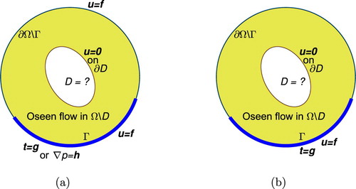
Corresponding to the situations in Figure 1(a) we have the inverse problems given by: (1) $\begin{array}{rl}\mu \mathrm{\Delta }\mathit{u}-\mathrm{\nabla }p& =u_0\varrho \frac{\mathrm{\partial }\mathit{u}}{\mathrm{\partial }{x}_1}\text{in}\mathrm{\Omega }\mathrm{\setminus }\overline{D},\end{array}$(1) (2) $\begin{array}{rl}\mathrm{\nabla }\cdot \mathit{u}& =0\text{in}\mathrm{\Omega }\mathrm{\setminus }\overline{D},\end{array}$(2) (3) $\begin{array}{rl}\mathit{u}& =\mathbf{0}\text{on}\mathrm{\partial }D,\end{array}$(3) (4) $\begin{array}{rl}\mathit{u}& =\mathit{f}\text{on}\mathrm{\partial }\mathrm{\Omega },\end{array}$(4) (5) $\begin{array}{rl}\mathit{t}& =\mathit{g}\text{on}\mathrm{\Gamma },\end{array}$(5) or (6) $\mathrm{\nabla }p=\mathit{h}\text{on}\mathrm{\Gamma },$(6) where Γ is a non-empty open portion of $\mathrm{\partial }\mathrm{\Omega }$, μ is the dynamic viscosity of the fluid, $\mathit{u}$ is the fluid velocity, p is the fluid pressure, $\varrho$ is the constant density of the incompressible fluid and $u_0$ is a given characteristic speed.

In the above, Equation (1(1) $\begin{array}{rl}\mu \mathrm{\Delta }\mathit{u}-\mathrm{\nabla }p& =u_0\varrho \frac{\mathrm{\partial }\mathit{u}}{\mathrm{\partial }{x}_1}\text{in}\mathrm{\Omega }\mathrm{\setminus }\overline{D},\end{array}$(1) ) represents the steady Oseen equations as a linearized version of the Navier–Stokes equations linearized with respect to the fixed velocity $u_0\mathit{i}$ in the $x_1$-direction, Equation (2(2) $\begin{array}{rl}\mathrm{\nabla }\cdot \mathit{u}& =0\text{in}\mathrm{\Omega }\mathrm{\setminus }\overline{D},\end{array}$(2) ) expresses the incompressibility of the fluid flow, Equation (3(3) $\begin{array}{rl}\mathit{u}& =\mathbf{0}\text{on}\mathrm{\partial }D,\end{array}$(3) ) is the no-slip condition on the obstacle D at rest, $\mathit{f}$ is a prescribed fluid velocity satisfying ${\int }_{\mathrm{\partial }\mathrm{\Omega }}\mathit{f}\cdot \mathit{n}\mathrm{d}S=0,$ $\mathit{h}$ is a prescribed pressure gradient and $\mathit{g}$ is a prescribed stress force, where (7) $\mathit{t}=\left(-p\mathbf{I}+\mu \left(\mathrm{\nabla }\mathit{u}+{\left(\mathrm{\nabla }\mathit{u}\right)}^T\right)\right)\mathit{n},$(7) $\mathit{n}$ is the outward unit normal to the boundary $\mathrm{\partial }\mathrm{\Omega }$ and $\mathbf{I}$ is the identity tensor.

Corresponding to the partial data situation in Figure 1(b) we have the more ill-posed inverse problem given by Equations (1(1) $\begin{array}{rl}\mu \mathrm{\Delta }\mathit{u}-\mathrm{\nabla }p& =u_0\varrho \frac{\mathrm{\partial }\mathit{u}}{\mathrm{\partial }{x}_1}\text{in}\mathrm{\Omega }\mathrm{\setminus }\overline{D},\end{array}$(1) )–(3(3) $\begin{array}{rl}\mathit{u}& =\mathbf{0}\text{on}\mathrm{\partial }D,\end{array}$(3) ), (5(5) $\begin{array}{rl}\mathit{t}& =\mathit{g}\text{on}\mathrm{\Gamma },\end{array}$(5) ) and (8) $\mathit{u}=\mathit{f}\text{on}\mathrm{\Gamma }.$(8) Assuming that $\mathit{f}\not\equiv \mathbf{0}$, the uniqueness of solution $(\mathit{u},p,D)$ of the inverse problems (1(1) $\begin{array}{rl}\mu \mathrm{\Delta }\mathit{u}-\mathrm{\nabla }p& =u_0\varrho \frac{\mathrm{\partial }\mathit{u}}{\mathrm{\partial }{x}_1}\text{in}\mathrm{\Omega }\mathrm{\setminus }\overline{D},\end{array}$(1) )–(5(5) $\begin{array}{rl}\mathit{t}& =\mathit{g}\text{on}\mathrm{\Gamma },\end{array}$(5) ) and (1(1) $\begin{array}{rl}\mu \mathrm{\Delta }\mathit{u}-\mathrm{\nabla }p& =u_0\varrho \frac{\mathrm{\partial }\mathit{u}}{\mathrm{\partial }{x}_1}\text{in}\mathrm{\Omega }\mathrm{\setminus }\overline{D},\end{array}$(1) )–(3(3) $\begin{array}{rl}\mathit{u}& =\mathbf{0}\text{on}\mathrm{\partial }D,\end{array}$(3) ), (5(5) $\begin{array}{rl}\mathit{t}& =\mathit{g}\text{on}\mathrm{\Gamma },\end{array}$(5) ), (8(8) $\mathit{u}=\mathit{f}\text{on}\mathrm{\Gamma }.$(8) ), follows from the unique continuation property for the Oseen system, see [3, 10, 11]. In addition, the uniqueness result also holds for the steady-state nonlinear Navier–Stokes equations $\mu \mathrm{\Delta }\mathit{u}-\mathrm{\nabla }p=\varrho (\mathit{u}\cdot \mathrm{\nabla })\mathit{u}$ generalizing their linearized version represented by the Oseen equations (1(1) $\begin{array}{rl}\mu \mathrm{\Delta }\mathit{u}-\mathrm{\nabla }p& =u_0\varrho \frac{\mathrm{\partial }\mathit{u}}{\mathrm{\partial }{x}_1}\text{in}\mathrm{\Omega }\mathrm{\setminus }\overline{D},\end{array}$(1) ), [10].

For the inverse problem (1(1) $\begin{array}{rl}\mu \mathrm{\Delta }\mathit{u}-\mathrm{\nabla }p& =u_0\varrho \frac{\mathrm{\partial }\mathit{u}}{\mathrm{\partial }{x}_1}\text{in}\mathrm{\Omega }\mathrm{\setminus }\overline{D},\end{array}$(1) )–(4(4) $\begin{array}{rl}\mathit{u}& =\mathit{f}\text{on}\mathrm{\partial }\mathrm{\Omega },\end{array}$(4) ), with prescribed pressure gradient (6(6) $\mathrm{\nabla }p=\mathit{h}\text{on}\mathrm{\Gamma },$(6) ) only a partial result concerning uniqueness is known in the two-dimensional case when $\mathrm{\partial }\mathrm{\Omega }$ contains a non-empty open segment ${\mathrm{\Gamma }}^{\mathrm{\prime }}$, see [10].

3. The method of fundamental solutions (MFS)

For simplicity, we only consider the two-dimensional case. The MFS for the exterior stationary Oseen fluid flow past an arbitrary obstacle has been recently introduced in [4]. For our interior problem in the annular domain $\mathrm{\Omega }\mathrm{\setminus }D$, it approximates the fluid velocity $\mathit{u}=(u_1,u_2)$ and pressure p as (9) $\begin{array}{rl}{u}_i\left(\mathit{x}\right)& =\sum _{j=1}^{M+N}\left({\alpha }_j{U}_{i1}(\mathit{x},{\mathit{\xi }}_j)+{\text{β}}_j{U}_{i2}(\mathit{x},{\mathit{\xi }}_j)\right),i=1,2,\mathit{x}\in \overline{\mathrm{\Omega }}\mathrm{\setminus }D,\end{array}$(9) (10) $\begin{array}{rl}p\left(\mathit{x}\right)& =\sum _{j=1}^{M+N}\left({\alpha }_j{P}_1(\mathit{x},{\mathit{\xi }}_j)+{\text{β}}_j{P}_2(\mathit{x},{\mathit{\xi }}_j)\right),i=1,2,\mathit{x}\in \overline{\mathrm{\Omega }}\mathrm{\setminus }D,\end{array}$(10) where the matrix U and the vector $\mathit{P}$ represent the fundamental solution of the Oseen system, which in two dimensions is given by $\begin{array}{rl}{U}_{11}(\mathit{x},{\mathit{x}}^{\mathrm{\prime }})& =\kappa {\mathrm{e}}^{\kappa (x-x^{\mathrm{\prime }})}\left[K_0\left(\kappa r\right)+\frac{x-x^{\mathrm{\prime }}}{r}{K}_1\left(\kappa r\right)\right]-\frac{x-x^{\mathrm{\prime }}}{r^2},\\ U_{12}(\mathit{x},{\mathit{x}}^{\mathrm{\prime }})& =U_{21}(\mathit{x},{\mathit{x}}^{\mathrm{\prime }})=-\frac{y-y^{\mathrm{\prime }}}{r}\left\{\frac{1}{r}-\kappa {\mathrm{e}}^{\kappa (x-x^{\mathrm{\prime }})}{K}_1\left(\kappa r\right)\right\},\\ U_{22}(\mathit{x},{\mathit{x}}^{\mathrm{\prime }})& =\frac{x-x^{\mathrm{\prime }}}{r^2}+\kappa {\mathrm{e}}^{\kappa (x-x^{\mathrm{\prime }})}\left[K_0\left(\kappa r\right)-\frac{x-x^{\mathrm{\prime }}}{r}{K}_1\left(\kappa r\right)\right].\end{array}$ For the pressure, we also define $P_1(\mathit{x},{\mathit{x}}^{\mathrm{\prime }})=\frac{(x-x^{\mathrm{\prime }})}{r^2},P_2(\mathit{x},{\mathit{x}}^{\mathrm{\prime }})=\frac{(y-y^{\mathrm{\prime }})}{r^2},$ where $\mathit{x}=(x,y)$, ${\mathit{x}}^{\mathrm{\prime }}=(x^{\mathrm{\prime }},y^{\mathrm{\prime }})$, $r=|\mathit{x}-{\mathit{x}}^{\mathrm{\prime }}|$, $\kappa =\varrho u_0/2\mu$, and $K_0$ and $K_1$ are the modified Bessel functions of the second kind of order zero and one, respectively.

Assuming that, for simplicity, Ω is a disk of radius R>0 centred at the origin containing the star-shaped obstacle D parameterized by (11) $D:=\left\{\mathrm{r}\left(\vartheta \right)\left(\cos \vartheta ,\sin \vartheta \right)|\vartheta \in [0,2\pi )\right\},\text{where}0<\mathrm{r}\left(\vartheta \right)<R,$(11) the source points $({\mathit{\xi }}_j{)}_{j=\overline{1,N+M}}$ in the MFS expansions (9(9) $\begin{array}{rl}{u}_i\left(\mathit{x}\right)& =\sum _{j=1}^{M+N}\left({\alpha }_j{U}_{i1}(\mathit{x},{\mathit{\xi }}_j)+{\text{β}}_j{U}_{i2}(\mathit{x},{\mathit{\xi }}_j)\right),i=1,2,\mathit{x}\in \overline{\mathrm{\Omega }}\mathrm{\setminus }D,\end{array}$(9) ) and (10(10) $\begin{array}{rl}p\left(\mathit{x}\right)& =\sum _{j=1}^{M+N}\left({\alpha }_j{P}_1(\mathit{x},{\mathit{\xi }}_j)+{\text{β}}_j{P}_2(\mathit{x},{\mathit{\xi }}_j)\right),i=1,2,\mathit{x}\in \overline{\mathrm{\Omega }}\mathrm{\setminus }D,\end{array}$(10) ) are taken as (12) $\begin{array}{rl}{\mathit{\xi }}_j& ={\eta }_{\mathrm{e}\mathrm{x}\mathrm{t}}R\left(\cos {\vartheta }_j,\sin {\vartheta }_j\right),{\vartheta }_j=2\pi (j-1)/M,j=\overline{1,M},{\eta }_{\mathrm{e}\mathrm{x}\mathrm{t}}>1,\end{array}$(12) (13) $\begin{array}{rl}{\mathit{\xi }}_{j+M}& ={\eta }_{\mathrm{i}\mathrm{n}\mathrm{t}}{\mathrm{r}}_j\left(\cos {\tilde{\vartheta }}_j,\sin {\tilde{\vartheta }}_j\right),{\tilde{\vartheta }}_j=2\pi (j-1)/N,\\ {\mathrm{r}}_j:& =\mathrm{r}\left({\tilde{\vartheta }}_j\right),j=\overline{1,N},0<{\eta }_{\mathrm{i}\mathrm{n}\mathrm{t}}<1.\end{array}$(13) The coefficient ${\eta }_{\mathrm{e}\mathrm{x}\mathrm{t}}>1$ is a dilation coefficient which is taken to be greater than one because the source points need to be taken outside the disk of radius R. 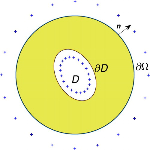The coefficient $0<{\eta }_{\mathrm{i}\mathrm{n}\mathrm{t}}<1$ is a contraction coefficient which is taken to be less than one because the source points need to be taken inside the star-shaped obstacle D. Note that all source points need to be outside the annular domain $\mathrm{\Omega }\mathrm{\setminus }D$, see Figure 2, such that the functions in (9(9) $\begin{array}{rl}{u}_i\left(\mathit{x}\right)& =\sum _{j=1}^{M+N}\left({\alpha }_j{U}_{i1}(\mathit{x},{\mathit{\xi }}_j)+{\text{β}}_j{U}_{i2}(\mathit{x},{\mathit{\xi }}_j)\right),i=1,2,\mathit{x}\in \overline{\mathrm{\Omega }}\mathrm{\setminus }D,\end{array}$(9) ) and (10(10) $\begin{array}{rl}p\left(\mathit{x}\right)& =\sum _{j=1}^{M+N}\left({\alpha }_j{P}_1(\mathit{x},{\mathit{\xi }}_j)+{\text{β}}_j{P}_2(\mathit{x},{\mathit{\xi }}_j)\right),i=1,2,\mathit{x}\in \overline{\mathrm{\Omega }}\mathrm{\setminus }D,\end{array}$(10) ) satisfy the Oseen system of Equations (1(1) $\begin{array}{rl}\mu \mathrm{\Delta }\mathit{u}-\mathrm{\nabla }p& =u_0\varrho \frac{\mathrm{\partial }\mathit{u}}{\mathrm{\partial }{x}_1}\text{in}\mathrm{\Omega }\mathrm{\setminus }\overline{D},\end{array}$(1) ) and (2(2) $\begin{array}{rl}\mathrm{\nabla }\cdot \mathit{u}& =0\text{in}\mathrm{\Omega }\mathrm{\setminus }\overline{D},\end{array}$(2) ).

Figure 2. Geometry of the problem. The ‘+’ denote the source points.

For expressing the stress force (7(7) $\mathit{t}=\left(-p\mathbf{I}+\mu \left(\mathrm{\nabla }\mathit{u}+{\left(\mathrm{\nabla }\mathit{u}\right)}^T\right)\right)\mathit{n},$(7) ) and the pressure gradient (6(6) $\mathrm{\nabla }p=\mathit{h}\text{on}\mathrm{\Gamma },$(6) ) we need the normal $\mathit{n}=(\cos \vartheta ,\sin \vartheta )$ and the gradients $\mathrm{\nabla }\mathit{u}$ and $\mathrm{\nabla }p$, which from (9(9) $\begin{array}{rl}{u}_i\left(\mathit{x}\right)& =\sum _{j=1}^{M+N}\left({\alpha }_j{U}_{i1}(\mathit{x},{\mathit{\xi }}_j)+{\text{β}}_j{U}_{i2}(\mathit{x},{\mathit{\xi }}_j)\right),i=1,2,\mathit{x}\in \overline{\mathrm{\Omega }}\mathrm{\setminus }D,\end{array}$(9) ), (10(10) $\begin{array}{rl}p\left(\mathit{x}\right)& =\sum _{j=1}^{M+N}\left({\alpha }_j{P}_1(\mathit{x},{\mathit{\xi }}_j)+{\text{β}}_j{P}_2(\mathit{x},{\mathit{\xi }}_j)\right),i=1,2,\mathit{x}\in \overline{\mathrm{\Omega }}\mathrm{\setminus }D,\end{array}$(10) ) and the expressions for the fundamental solution yield the formulæ given in the Appendix.

From (7(7) $\mathit{t}=\left(-p\mathbf{I}+\mu \left(\mathrm{\nabla }\mathit{u}+{\left(\mathrm{\nabla }\mathit{u}\right)}^T\right)\right)\mathit{n},$(7) ), we have componentwise that $t_1=-p{n}_1+2\frac{\mathrm{\partial }{u}_1}{\mathrm{\partial }x}{n}_1+\left(\frac{\mathrm{\partial }{u}_2}{\mathrm{\partial }x}+\frac{\mathrm{\partial }{u}_1}{\mathrm{\partial }y}\right)n_2,t_2=-p{n}_2+\left(\frac{\mathrm{\partial }{u}_1}{\mathrm{\partial }y}+\frac{\mathrm{\partial }{u}_2}{\mathrm{\partial }x}\right)n_1+2\frac{\mathrm{\partial }{u}_2}{\mathrm{\partial }y}{n}_2,$ where $\mathit{n}=(n_1,n_2)$. Then, using (9(9) $\begin{array}{rl}{u}_i\left(\mathit{x}\right)& =\sum _{j=1}^{M+N}\left({\alpha }_j{U}_{i1}(\mathit{x},{\mathit{\xi }}_j)+{\text{β}}_j{U}_{i2}(\mathit{x},{\mathit{\xi }}_j)\right),i=1,2,\mathit{x}\in \overline{\mathrm{\Omega }}\mathrm{\setminus }D,\end{array}$(9) ) and (10(10) $\begin{array}{rl}p\left(\mathit{x}\right)& =\sum _{j=1}^{M+N}\left({\alpha }_j{P}_1(\mathit{x},{\mathit{\xi }}_j)+{\text{β}}_j{P}_2(\mathit{x},{\mathit{\xi }}_j)\right),i=1,2,\mathit{x}\in \overline{\mathrm{\Omega }}\mathrm{\setminus }D,\end{array}$(10) ) we obtain $\begin{array}{rl}{t}_1\left(\mathit{x}\right)& =\sum _{j=1}^{M+N}\left({\alpha }_j{D}_{11}(\mathit{x},{\mathit{\xi }}_j)+{\text{β}}_j{D}_{12}(\mathit{x},{\mathit{\xi }}_j)\right),\\ t_2\left(\mathit{x}\right)& =\sum _{j=1}^{M+N}\left({\alpha }_j{D}_{21}(\mathit{x},{\mathit{\xi }}_j)+{\text{β}}_j{D}_{22}(\mathit{x},{\mathit{\xi }}_j)\right),\end{array}$ where $\begin{array}{rl}{D}_{11}& =-P_1{n}_1+2\frac{\mathrm{\partial }{U}_{11}}{\mathrm{\partial }x}{n}_1+\left(\frac{\mathrm{\partial }{U}_{21}}{\mathrm{\partial }x}+\frac{\mathrm{\partial }{U}_{11}}{\mathrm{\partial }y}\right)n_2,\\ D_{12}& =-P_2{n}_1+2\frac{\mathrm{\partial }{U}_{12}}{\mathrm{\partial }x}{n}_1+\left(\frac{\mathrm{\partial }{U}_{22}}{\mathrm{\partial }x}+\frac{\mathrm{\partial }{U}_{12}}{\mathrm{\partial }y}\right)n_2,\\ D_{21}& =-P_1{n}_2+\left(\frac{\mathrm{\partial }{U}_{11}}{\mathrm{\partial }y}+\frac{\mathrm{\partial }{U}_{21}}{\mathrm{\partial }x}\right)n_1+2\frac{\mathrm{\partial }{U}_{21}}{\mathrm{\partial }y}{n}_2,\\ D_{22}& =-P_2{n}_2+\left(\frac{\mathrm{\partial }{U}_{12}}{\mathrm{\partial }y}+\frac{\mathrm{\partial }{U}_{22}}{\mathrm{\partial }x}\right)n_1+2\frac{\mathrm{\partial }{U}_{22}}{\mathrm{\partial }y}{n}_2.\end{array}$ We now consider the boundary collocation points (14) ${\mathit{x}}_j=R\left(\cos {\vartheta }_j,\sin {\vartheta }_j\right),j=\overline{1,M}\text{on}\mathrm{\partial }\mathrm{\Omega },$(14) and (15) ${\mathit{x}}_{M+j}={\mathrm{r}}_j\left(\cos {\tilde{\vartheta }}_j,\sin {\tilde{\vartheta }}_j\right),j=\overline{1,N}\text{on}\mathrm{\partial }D.$(15) We also assume, without loss of generality, that Γ contains the first $0<M_1\le M$ boundary collocation points $({\mathit{x}}_j{)}_{j=\overline{1,M_1}}$.

For the inverse problems (1(1) $\begin{array}{rl}\mu \mathrm{\Delta }\mathit{u}-\mathrm{\nabla }p& =u_0\varrho \frac{\mathrm{\partial }\mathit{u}}{\mathrm{\partial }{x}_1}\text{in}\mathrm{\Omega }\mathrm{\setminus }\overline{D},\end{array}$(1) )–(5(5) $\begin{array}{rl}\mathit{t}& =\mathit{g}\text{on}\mathrm{\Gamma },\end{array}$(5) ) or (1(1) $\begin{array}{rl}\mu \mathrm{\Delta }\mathit{u}-\mathrm{\nabla }p& =u_0\varrho \frac{\mathrm{\partial }\mathit{u}}{\mathrm{\partial }{x}_1}\text{in}\mathrm{\Omega }\mathrm{\setminus }\overline{D},\end{array}$(1) )–(4(4) $\begin{array}{rl}\mathit{u}& =\mathit{f}\text{on}\mathrm{\partial }\mathrm{\Omega },\end{array}$(4) ), (6(6) $\mathrm{\nabla }p=\mathit{h}\text{on}\mathrm{\Gamma },$(6) ), illustrated in Figure 1(a), we minimize the nonlinear least-squares functionals (16) $\begin{array}{rl}{\mathcal{F}}_1(\mathit{\alpha },\text{β},r,{\eta }_{\mathrm{i}\mathrm{n}\mathrm{t}},{\eta }_{\mathrm{e}\mathrm{x}\mathrm{t}})& =\parallel \mathit{u}{\parallel }_{L^2\left(\mathrm{\partial }D\right)}^2+\parallel \mathit{u}-\mathit{f}{\parallel }_{L^2\left(\mathrm{\partial }\mathrm{\Omega }\right)}^2+\parallel \mathit{t}-{\mathit{g}}^{\epsilon }{\parallel }_{L^2\left(\mathrm{\Gamma }\right)}^2\\ & +\mathcal{R}(\mathit{\alpha },\text{β},\mathrm{\nabla }\mathrm{r};{\mu }_1,{\mu }_2)\end{array}$(16) or (17) $\begin{array}{rl}{\mathcal{F}}_2(\mathit{\alpha },\text{β},r,{\eta }_{\mathrm{i}\mathrm{n}\mathrm{t}},{\eta }_{\mathrm{e}\mathrm{x}\mathrm{t}})& =\parallel \mathit{u}{\parallel }_{L^2\left(\mathrm{\partial }D\right)}^2+\parallel \mathit{u}-\mathit{f}{\parallel }_{L^2\left(\mathrm{\partial }\mathrm{\Omega }\right)}^2+\parallel \mathrm{\nabla }p-{\mathit{h}}^{\epsilon }{\parallel }_{L^2\left(\mathrm{\Gamma }\right)}^2\\ & +\mathcal{R}(\mathit{\alpha },\text{β},\mathrm{\nabla }\mathrm{r};{\mu }_1,{\mu }_2),\end{array}$(17) where $\mathit{\alpha }=({\alpha }_j{)}_{j=\overline{1,M+N}},\text{β}=({\text{β}}_j{)}_{j=\overline{1,M+N}}$, noise is introduced in (5(5) $\begin{array}{rl}\mathit{t}& =\mathit{g}\text{on}\mathrm{\Gamma },\end{array}$(5) ) or (6(6) $\mathrm{\nabla }p=\mathit{h}\text{on}\mathrm{\Gamma },$(6) ) (representing boundary measurements of the stress force or the pressure gradient) as (18) ${\mathit{g}}^{\epsilon }=\mathit{g}+\mathit{\epsilon }$(18) or (19) ${\mathit{h}}^{\epsilon }=\mathit{h}+\mathit{\epsilon },$(19) where $\mathit{\epsilon }$ represents some noise, and $\mathcal{R}$ is a regularization term given by (20) $\mathcal{R}(\mathit{\alpha },\text{β},\mathrm{\nabla }\mathrm{r};{\mu }_1,{\mu }_2)={\mu }_1\left(|\mathit{\alpha }{|}^2+|\text{β}{|}^2\right)+{\mu }_2\parallel \mathrm{\nabla }\mathrm{r}{\parallel }_{L^2\left(\mathrm{\partial }D\right)}^2,$(20) where ${\mu }_1$ and ${\mu }_2$ are positive regularization parameters which need to be prescribed, e.g. by trial and error or using some criterion such as the L-surface method [12], or the L-curve criterion if we take ${\mu }_1={\mu }_2=\mu$, or ${\mu }_1=0$ and vary ${\mu }_2$, or ${\mu }_2=0$ and vary ${\mu }_1$, [13]. Other multi-parameter regularization choices based on the discrepancy principle can also be applied, [14]. The first three terms in the right-hand side of Equation (16(16) $\begin{array}{rl}{\mathcal{F}}_1(\mathit{\alpha },\text{β},r,{\eta }_{\mathrm{i}\mathrm{n}\mathrm{t}},{\eta }_{\mathrm{e}\mathrm{x}\mathrm{t}})& =\parallel \mathit{u}{\parallel }_{L^2\left(\mathrm{\partial }D\right)}^2+\parallel \mathit{u}-\mathit{f}{\parallel }_{L^2\left(\mathrm{\partial }\mathrm{\Omega }\right)}^2+\parallel \mathit{t}-{\mathit{g}}^{\epsilon }{\parallel }_{L^2\left(\mathrm{\Gamma }\right)}^2\\ & +\mathcal{R}(\mathit{\alpha },\text{β},\mathrm{\nabla }\mathrm{r};{\mu }_1,{\mu }_2)\end{array}$(16) ) and the third term in the right-hand side of Equation (17(17) $\begin{array}{rl}{\mathcal{F}}_2(\mathit{\alpha },\text{β},r,{\eta }_{\mathrm{i}\mathrm{n}\mathrm{t}},{\eta }_{\mathrm{e}\mathrm{x}\mathrm{t}})& =\parallel \mathit{u}{\parallel }_{L^2\left(\mathrm{\partial }D\right)}^2+\parallel \mathit{u}-\mathit{f}{\parallel }_{L^2\left(\mathrm{\partial }\mathrm{\Omega }\right)}^2+\parallel \mathrm{\nabla }p-{\mathit{h}}^{\epsilon }{\parallel }_{L^2\left(\mathrm{\Gamma }\right)}^2\\ & +\mathcal{R}(\mathit{\alpha },\text{β},\mathrm{\nabla }\mathrm{r};{\mu }_1,{\mu }_2),\end{array}$(17) ) impose the boundary conditions (3(3) $\begin{array}{rl}\mathit{u}& =\mathbf{0}\text{on}\mathrm{\partial }D,\end{array}$(3) )–(6(6) $\mathrm{\nabla }p=\mathit{h}\text{on}\mathrm{\Gamma },$(6) ) in a least-squares sense, while the functions $\mathit{u}\left(\mathit{x}\right)$ and $p\left(\mathit{x}\right)$ are parameterized using the vectors $\mathit{\alpha }$ and $\text{β}$ in the MFS approximations (9(9) $\begin{array}{rl}{u}_i\left(\mathit{x}\right)& =\sum _{j=1}^{M+N}\left({\alpha }_j{U}_{i1}(\mathit{x},{\mathit{\xi }}_j)+{\text{β}}_j{U}_{i2}(\mathit{x},{\mathit{\xi }}_j)\right),i=1,2,\mathit{x}\in \overline{\mathrm{\Omega }}\mathrm{\setminus }D,\end{array}$(9) ) and (10(10) $\begin{array}{rl}p\left(\mathit{x}\right)& =\sum _{j=1}^{M+N}\left({\alpha }_j{P}_1(\mathit{x},{\mathit{\xi }}_j)+{\text{β}}_j{P}_2(\mathit{x},{\mathit{\xi }}_j)\right),i=1,2,\mathit{x}\in \overline{\mathrm{\Omega }}\mathrm{\setminus }D,\end{array}$(10) ).

Noise can also be introduced in the boundary fluid velocity data (4(4) $\begin{array}{rl}\mathit{u}& =\mathit{f}\text{on}\mathrm{\partial }\mathrm{\Omega },\end{array}$(4) ), but, for simplicity, we do not consider these errors herein.

For the inverse problem (1(1) $\begin{array}{rl}\mu \mathrm{\Delta }\mathit{u}-\mathrm{\nabla }p& =u_0\varrho \frac{\mathrm{\partial }\mathit{u}}{\mathrm{\partial }{x}_1}\text{in}\mathrm{\Omega }\mathrm{\setminus }\overline{D},\end{array}$(1) )–(3(3) $\begin{array}{rl}\mathit{u}& =\mathbf{0}\text{on}\mathrm{\partial }D,\end{array}$(3) ), (5(5) $\begin{array}{rl}\mathit{t}& =\mathit{g}\text{on}\mathrm{\Gamma },\end{array}$(5) ) and (8(8) $\mathit{u}=\mathit{f}\text{on}\mathrm{\Gamma }.$(8) ), illustrated in Figure 1(b), we minimize (21) ${\mathcal{F}}_3(\mathit{\alpha },\text{β},r,{\eta }_{\mathrm{i}\mathrm{n}\mathrm{t}},{\eta }_{\mathrm{e}\mathrm{x}\mathrm{t}})=\parallel \mathit{u}{\parallel }_{L^2\left(\mathrm{\partial }D\right)}^2+\parallel \mathit{u}-\mathit{f}{\parallel }_{L^2\left(\mathrm{\Gamma }\right)}^2+\parallel \mathit{t}-{\mathit{g}}^{\epsilon }{\parallel }_{L^2\left(\mathrm{\Gamma }\right)}^2+\mathcal{R}(\mathit{\alpha },\text{β},\mathrm{\nabla }\mathrm{r};{\mu }_1,{\mu }_2).$(21) On discretizing the norms in (16(16) $\begin{array}{rl}{\mathcal{F}}_1(\mathit{\alpha },\text{β},r,{\eta }_{\mathrm{i}\mathrm{n}\mathrm{t}},{\eta }_{\mathrm{e}\mathrm{x}\mathrm{t}})& =\parallel \mathit{u}{\parallel }_{L^2\left(\mathrm{\partial }D\right)}^2+\parallel \mathit{u}-\mathit{f}{\parallel }_{L^2\left(\mathrm{\partial }\mathrm{\Omega }\right)}^2+\parallel \mathit{t}-{\mathit{g}}^{\epsilon }{\parallel }_{L^2\left(\mathrm{\Gamma }\right)}^2\\ & +\mathcal{R}(\mathit{\alpha },\text{β},\mathrm{\nabla }\mathrm{r};{\mu }_1,{\mu }_2)\end{array}$(16) ), (17(17) $\begin{array}{rl}{\mathcal{F}}_2(\mathit{\alpha },\text{β},r,{\eta }_{\mathrm{i}\mathrm{n}\mathrm{t}},{\eta }_{\mathrm{e}\mathrm{x}\mathrm{t}})& =\parallel \mathit{u}{\parallel }_{L^2\left(\mathrm{\partial }D\right)}^2+\parallel \mathit{u}-\mathit{f}{\parallel }_{L^2\left(\mathrm{\partial }\mathrm{\Omega }\right)}^2+\parallel \mathrm{\nabla }p-{\mathit{h}}^{\epsilon }{\parallel }_{L^2\left(\mathrm{\Gamma }\right)}^2\\ & +\mathcal{R}(\mathit{\alpha },\text{β},\mathrm{\nabla }\mathrm{r};{\mu }_1,{\mu }_2),\end{array}$(17) ) and (21(21) ${\mathcal{F}}_3(\mathit{\alpha },\text{β},r,{\eta }_{\mathrm{i}\mathrm{n}\mathrm{t}},{\eta }_{\mathrm{e}\mathrm{x}\mathrm{t}})=\parallel \mathit{u}{\parallel }_{L^2\left(\mathrm{\partial }D\right)}^2+\parallel \mathit{u}-\mathit{f}{\parallel }_{L^2\left(\mathrm{\Gamma }\right)}^2+\parallel \mathit{t}-{\mathit{g}}^{\epsilon }{\parallel }_{L^2\left(\mathrm{\Gamma }\right)}^2+\mathcal{R}(\mathit{\alpha },\text{β},\mathrm{\nabla }\mathrm{r};{\mu }_1,{\mu }_2).$(21) ), and using the MFS approximations (9(9) $\begin{array}{rl}{u}_i\left(\mathit{x}\right)& =\sum _{j=1}^{M+N}\left({\alpha }_j{U}_{i1}(\mathit{x},{\mathit{\xi }}_j)+{\text{β}}_j{U}_{i2}(\mathit{x},{\mathit{\xi }}_j)\right),i=1,2,\mathit{x}\in \overline{\mathrm{\Omega }}\mathrm{\setminus }D,\end{array}$(9) ) and (10(10) $\begin{array}{rl}p\left(\mathit{x}\right)& =\sum _{j=1}^{M+N}\left({\alpha }_j{P}_1(\mathit{x},{\mathit{\xi }}_j)+{\text{β}}_j{P}_2(\mathit{x},{\mathit{\xi }}_j)\right),i=1,2,\mathit{x}\in \overline{\mathrm{\Omega }}\mathrm{\setminus }D,\end{array}$(10) ), we obtain (22) $\begin{array}{rl}{\mathcal{F}}_1(\mathit{\alpha },\text{β},\mathbf{r},{\eta }_{\mathrm{i}\mathrm{n}\mathrm{t}},{\eta }_{\mathrm{e}\mathrm{x}\mathrm{t}})& =T_0(\mathit{\alpha },\text{β},\mathbf{r},{\eta }_{\mathrm{i}\mathrm{n}\mathrm{t}},{\eta }_{\mathrm{e}\mathrm{x}\mathrm{t}})+T_{\mathit{f}}(\mathit{\alpha },\text{β},\mathbf{r},{\eta }_{\mathrm{i}\mathrm{n}\mathrm{t}},{\eta }_{\mathrm{e}\mathrm{x}\mathrm{t}})\\ & +T_{{\mathit{g}}^{\epsilon }}(\mathit{\alpha },\text{β},\mathbf{r},{\eta }_{\mathrm{i}\mathrm{n}\mathrm{t}},{\eta }_{\mathrm{e}\mathrm{x}\mathrm{t}})+\mathcal{R}(\mathit{\alpha },\text{β},{\mathbf{r}}^{\mathrm{\prime }};{\mu }_1,{\mu }_2),\end{array}$(22) (23) $\begin{array}{rl}{\mathcal{F}}_2(\mathit{\alpha },\text{β},\mathbf{r},{\eta }_{\mathrm{i}\mathrm{n}\mathrm{t}},{\eta }_{\mathrm{e}\mathrm{x}\mathrm{t}})& =T_0(\mathit{\alpha },\text{β},\mathbf{r},{\eta }_{\mathrm{i}\mathrm{n}\mathrm{t}},{\eta }_{\mathrm{e}\mathrm{x}\mathrm{t}})+T_{\mathit{f}}(\mathit{\alpha },\text{β},\mathbf{r},{\eta }_{\mathrm{i}\mathrm{n}\mathrm{t}},{\eta }_{\mathrm{e}\mathrm{x}\mathrm{t}})\\ & +T_{{\mathit{h}}^{\epsilon }}(\mathit{\alpha },\text{β},\mathbf{r},{\eta }_{\mathrm{i}\mathrm{n}\mathrm{t}},{\eta }_{\mathrm{e}\mathrm{x}\mathrm{t}})+\mathcal{R}(\mathit{\alpha },\text{β},{\mathbf{r}}^{\mathrm{\prime }};{\mu }_1,{\mu }_2),\end{array}$(23) (24) $\begin{array}{rl}{\mathcal{F}}_3(\mathit{\alpha },\text{β},\mathbf{r},{\eta }_{\mathrm{i}\mathrm{n}\mathrm{t}},{\eta }_{\mathrm{e}\mathrm{x}\mathrm{t}})& =T_0(\mathit{\alpha },\text{β},\mathbf{r},{\eta }_{\mathrm{i}\mathrm{n}\mathrm{t}},{\eta }_{\mathrm{e}\mathrm{x}\mathrm{t}})+T_{\mathit{f}}^1(\mathit{\alpha },\text{β},\mathbf{r},{\eta }_{\mathrm{i}\mathrm{n}\mathrm{t}},{\eta }_{\mathrm{e}\mathrm{x}\mathrm{t}})\\ & +T_{{\mathit{g}}^{\epsilon }}(\mathit{\alpha },\text{β},\mathbf{r},{\eta }_{\mathrm{i}\mathrm{n}\mathrm{t}},{\eta }_{\mathrm{e}\mathrm{x}\mathrm{t}})+\mathcal{R}(\mathit{\alpha },\text{β},{\mathbf{r}}^{\mathrm{\prime }};{\mu }_1,{\mu }_2),\end{array}$(24) respectively, where (25) $\mathcal{R}(\mathit{\alpha },\text{β},{\mathbf{r}}^{\mathrm{\prime }};{\mu }_1,{\mu }_2)={\mu }_1\left(|\mathit{\alpha }{|}^2+|\text{β}{|}^2\right)+{\mu }_2\sum _{j=2}^N{\left({\mathrm{r}}_j-{\mathrm{r}}_{j-1}\right)}^2,$(25) $\begin{array}{rl}{T}_0(\mathit{\alpha },\text{β},\mathbf{r},{\eta }_{\mathrm{i}\mathrm{n}\mathrm{t}},{\eta }_{\mathrm{e}\mathrm{x}\mathrm{t}})& =\sum _{i=1}^2\sum _{k=1}^N{\left[\sum _{j=1}^{M+N}\left({\alpha }_j{U}_{i1}({\mathit{x}}_{M+k},{\mathit{\xi }}_j)+{\text{β}}_j{U}_{i2}({\mathit{x}}_{M+k},{\mathit{\xi }}_j)\right)\right]}^2,\\ T_{\mathit{f}}(\mathit{\alpha },\text{β},\mathbf{r},{\eta }_{\mathrm{i}\mathrm{n}\mathrm{t}},{\eta }_{\mathrm{e}\mathrm{x}\mathrm{t}})& =\sum _{i=1}^2\sum _{k=1}^M{\left[\sum _{j=1}^{M+N}\left({\alpha }_j{U}_{i1}({\mathit{x}}_k,{\mathit{\xi }}_j)+{\text{β}}_j{U}_{i2}({\mathit{x}}_k,{\mathit{\xi }}_j)\right)-f_i\left({\mathit{x}}_k\right)\right]}^2,\\ T_{{\mathit{g}}^{\epsilon }}(\mathit{\alpha },\text{β},\mathbf{r},{\eta }_{\mathrm{i}\mathrm{n}\mathrm{t}},{\eta }_{\mathrm{e}\mathrm{x}\mathrm{t}})& =\sum _{i=1}^2\sum _{k=1}^{M_1}{\left[\sum _{j=1}^{M+N}\left({\alpha }_j{D}_{i1}({\mathit{x}}_k,{\mathit{\xi }}_j)+{\text{β}}_j{D}_{i2}({\mathit{x}}_k,{\mathit{\xi }}_j)\right)-g_i^{\epsilon }\left({\mathit{x}}_k\right)\right]}^2,\\ T_{{\mathit{h}}^{\epsilon }}(\mathit{\alpha },\text{β},\mathbf{r},{\eta }_{\mathrm{i}\mathrm{n}\mathrm{t}},{\eta }_{\mathrm{e}\mathrm{x}\mathrm{t}})& =\sum _{i=1}^2\sum _{k=1}^{M_1}{\left[\sum _{j=1}^{M+N}\left({\alpha }_j{E}_{i1}({\mathit{x}}_k,{\mathit{\xi }}_j)+{\text{β}}_j{E}_{i2}({\mathit{x}}_k,{\mathit{\xi }}_j)\right)-h_i^{\epsilon }\left({\mathit{x}}_k\right)\right]}^2,\\ T_{\mathit{f}}^1(\mathit{\alpha },\text{β},\mathbf{r},{\eta }_{\mathrm{i}\mathrm{n}\mathrm{t}},{\eta }_{\mathrm{e}\mathrm{x}\mathrm{t}})& =\sum _{i=1}^2\sum _{k=1}^{M_1}{\left[\sum _{j=1}^{M+N}\left({\alpha }_j{U}_{i1}({\mathit{x}}_k,{\mathit{\xi }}_j)+{\text{β}}_j{U}_{i2}({\mathit{x}}_k,{\mathit{\xi }}_j)\right)-f_i\left({\mathit{x}}_k\right)\right]}^2,\end{array}$ where $E_{1i}=\mathrm{\partial }{P}_i/\mathrm{\partial }x$ and $E_{2i}=\mathrm{\partial }{P}_i/\mathrm{\partial }y$ for i = 1, 2.

As in the analysis of [13], performed for inverse scattering, the regularization term (20(20) $\mathcal{R}(\mathit{\alpha },\text{β},\mathrm{\nabla }\mathrm{r};{\mu }_1,{\mu }_2)={\mu }_1\left(|\mathit{\alpha }{|}^2+|\text{β}{|}^2\right)+{\mu }_2\parallel \mathrm{\nabla }\mathrm{r}{\parallel }_{L^2\left(\mathrm{\partial }D\right)}^2,$(20) ) (or its discretized version (25(25) $\mathcal{R}(\mathit{\alpha },\text{β},{\mathbf{r}}^{\mathrm{\prime }};{\mu }_1,{\mu }_2)={\mu }_1\left(|\mathit{\alpha }{|}^2+|\text{β}{|}^2\right)+{\mu }_2\sum _{j=2}^N{\left({\mathrm{r}}_j-{\mathrm{r}}_{j-1}\right)}^2,$(25) )) is included in order to achieve stability, corresponding to the ${\ell }^2$-norm of the MFS coefficients $\mathit{\alpha }$ and $\text{β}$ and the gradient $H^1$-norm of the smooth obstacle polar radius $\mathrm{r}\left(\vartheta \right),\vartheta \in [0,2\pi )$. The minimization of (16(16) $\begin{array}{rl}{\mathcal{F}}_1(\mathit{\alpha },\text{β},r,{\eta }_{\mathrm{i}\mathrm{n}\mathrm{t}},{\eta }_{\mathrm{e}\mathrm{x}\mathrm{t}})& =\parallel \mathit{u}{\parallel }_{L^2\left(\mathrm{\partial }D\right)}^2+\parallel \mathit{u}-\mathit{f}{\parallel }_{L^2\left(\mathrm{\partial }\mathrm{\Omega }\right)}^2+\parallel \mathit{t}-{\mathit{g}}^{\epsilon }{\parallel }_{L^2\left(\mathrm{\Gamma }\right)}^2\\ & +\mathcal{R}(\mathit{\alpha },\text{β},\mathrm{\nabla }\mathrm{r};{\mu }_1,{\mu }_2)\end{array}$(16) ), (17(17) $\begin{array}{rl}{\mathcal{F}}_2(\mathit{\alpha },\text{β},r,{\eta }_{\mathrm{i}\mathrm{n}\mathrm{t}},{\eta }_{\mathrm{e}\mathrm{x}\mathrm{t}})& =\parallel \mathit{u}{\parallel }_{L^2\left(\mathrm{\partial }D\right)}^2+\parallel \mathit{u}-\mathit{f}{\parallel }_{L^2\left(\mathrm{\partial }\mathrm{\Omega }\right)}^2+\parallel \mathrm{\nabla }p-{\mathit{h}}^{\epsilon }{\parallel }_{L^2\left(\mathrm{\Gamma }\right)}^2\\ & +\mathcal{R}(\mathit{\alpha },\text{β},\mathrm{\nabla }\mathrm{r};{\mu }_1,{\mu }_2),\end{array}$(17) ) and (21(21) ${\mathcal{F}}_3(\mathit{\alpha },\text{β},r,{\eta }_{\mathrm{i}\mathrm{n}\mathrm{t}},{\eta }_{\mathrm{e}\mathrm{x}\mathrm{t}})=\parallel \mathit{u}{\parallel }_{L^2\left(\mathrm{\partial }D\right)}^2+\parallel \mathit{u}-\mathit{f}{\parallel }_{L^2\left(\mathrm{\Gamma }\right)}^2+\parallel \mathit{t}-{\mathit{g}}^{\epsilon }{\parallel }_{L^2\left(\mathrm{\Gamma }\right)}^2+\mathcal{R}(\mathit{\alpha },\text{β},\mathrm{\nabla }\mathrm{r};{\mu }_1,{\mu }_2).$(21) ) subject to the simple bounds on the variables (26) $\begin{array}{rl}-{10}^5& \le {\alpha }_j\le {10}^5,-{10}^5\le {\text{β}}_j\le {10}^5,j=\overline{1,M+N},\\ 0& <{\mathrm{r}}_{\mathrm{m}\mathrm{i}\mathrm{n}}\le {\mathrm{r}}_{\ell }\le {\mathrm{r}}_{\mathrm{m}\mathrm{a}\mathrm{x}}<R,\ell =\overline{1,N},\\ 0.1& \le {\eta }_{\mathrm{i}\mathrm{n}\mathrm{t}}\le 0.99,1.1\le {\eta }_{\mathrm{e}\mathrm{x}\mathrm{t}}\le 2,\end{array}$(26) where ${\mathrm{r}}_{\mathrm{m}\mathrm{i}\mathrm{n}}$ and ${\mathrm{r}}_{\mathrm{m}\mathrm{a}\mathrm{x}}$ are lower and upper bounds on the size of the obstacle D, respectively, is performed using the MATLAB${}^{\copyright }$ [15] optimization toolbox routine lsqnonlin.

4. Numerical examples

We take the radius of the disk $\mathrm{\Omega }=B(\mathbf{0};R)$ to be R = 2.5, and, in general, consider the case of full data when Γ is the whole of the boundary $\mathrm{\partial }\mathrm{\Omega }$. In this case, the boundary fluid velocity conditions (4(4) $\begin{array}{rl}\mathit{u}& =\mathit{f}\text{on}\mathrm{\partial }\mathrm{\Omega },\end{array}$(4) ) and (8(8) $\mathit{u}=\mathit{f}\text{on}\mathrm{\Gamma }.$(8) ) coincide. Limited aperture data (5(5) $\begin{array}{rl}\mathit{t}& =\mathit{g}\text{on}\mathrm{\Gamma },\end{array}$(5) ) or (6(6) $\mathrm{\nabla }p=\mathit{h}\text{on}\mathrm{\Gamma },$(6) ) taken over an arc $\mathrm{\Gamma }\subset \mathrm{\partial }\mathrm{\Omega }=\mathrm{\partial }B(\mathbf{0};R)$, will also be considered for the first example below.

For an arbitrary star-shaped obstacle (11(11) $D:=\left\{\mathrm{r}\left(\vartheta \right)\left(\cos \vartheta ,\sin \vartheta \right)|\vartheta \in [0,2\pi )\right\},\text{where}0<\mathrm{r}\left(\vartheta \right)<R,$(11) ), the additional input data (5(5) $\begin{array}{rl}\mathit{t}& =\mathit{g}\text{on}\mathrm{\Gamma },\end{array}$(5) ) or (6(6) $\mathrm{\nabla }p=\mathit{h}\text{on}\mathrm{\Gamma },$(6) ), representing the stress force or the pressure gradient on Γ, is numerically simulated by first solving the direct problem (1(1) $\begin{array}{rl}\mu \mathrm{\Delta }\mathit{u}-\mathrm{\nabla }p& =u_0\varrho \frac{\mathrm{\partial }\mathit{u}}{\mathrm{\partial }{x}_1}\text{in}\mathrm{\Omega }\mathrm{\setminus }\overline{D},\end{array}$(1) )–(4(4) $\begin{array}{rl}\mathit{u}& =\mathit{f}\text{on}\mathrm{\partial }\mathrm{\Omega },\end{array}$(4) ) with known D using the MFS, while ensuring that an inverse crime is not committed. We take [2] (27) $\mathit{u}(x,y)=\mathit{f}(x,y)=(-y,x),(x,y)\in \mathrm{\partial }\mathrm{\Omega },$(27) for the specified boundary velocity in (4(4) $\begin{array}{rl}\mathit{u}& =\mathit{f}\text{on}\mathrm{\partial }\mathrm{\Omega },\end{array}$(4) ). We also take $\varrho =1$, $\mu =1$ and $u_0=0.5$.

The data (5(5) $\begin{array}{rl}\mathit{t}& =\mathit{g}\text{on}\mathrm{\Gamma },\end{array}$(5) ) and (6(6) $\mathrm{\nabla }p=\mathit{h}\text{on}\mathrm{\Gamma },$(6) ) is perturbed by multiplicative noise (28) ${\mathit{g}}^{\epsilon }\left({\mathit{x}}_k\right)=(1+{\chi }_k\mathrm{p})\mathit{g}\left({\mathit{x}}_k\right),{\mathit{h}}^{\epsilon }\left({\mathit{x}}_k\right)=(1+{\chi }_k\mathrm{p})\mathit{h}\left({\mathit{x}}_k\right),k=\overline{1,M_1},$(28) where $\mathrm{p}$ is the percentage of noise and ${\chi }_k$ is a pseudo-random noisy variable generated from a uniform distribution in [$-1$,1].

We consider both inverse problems (1(1) $\begin{array}{rl}\mu \mathrm{\Delta }\mathit{u}-\mathrm{\nabla }p& =u_0\varrho \frac{\mathrm{\partial }\mathit{u}}{\mathrm{\partial }{x}_1}\text{in}\mathrm{\Omega }\mathrm{\setminus }\overline{D},\end{array}$(1) )–(5(5) $\begin{array}{rl}\mathit{t}& =\mathit{g}\text{on}\mathrm{\Gamma },\end{array}$(5) ) and (1(1) $\begin{array}{rl}\mu \mathrm{\Delta }\mathit{u}-\mathrm{\nabla }p& =u_0\varrho \frac{\mathrm{\partial }\mathit{u}}{\mathrm{\partial }{x}_1}\text{in}\mathrm{\Omega }\mathrm{\setminus }\overline{D},\end{array}$(1) )–(4(4) $\begin{array}{rl}\mathit{u}& =\mathit{f}\text{on}\mathrm{\partial }\mathrm{\Omega },\end{array}$(4) ) and (6(6) $\mathrm{\nabla }p=\mathit{h}\text{on}\mathrm{\Gamma },$(6) ). We have a total of $2(M+M_1)+2N$ equations ($2M$ equations for boundary conditions (4(4) $\begin{array}{rl}\mathit{u}& =\mathit{f}\text{on}\mathrm{\partial }\mathrm{\Omega },\end{array}$(4) ), $2N$ equations for boundary conditions (3(3) $\begin{array}{rl}\mathit{u}& =\mathbf{0}\text{on}\mathrm{\partial }D,\end{array}$(3) ) and $2M_1$ equations for boundary conditions (5(5) $\begin{array}{rl}\mathit{t}& =\mathit{g}\text{on}\mathrm{\Gamma },\end{array}$(5) ) or (6(6) $\mathrm{\nabla }p=\mathit{h}\text{on}\mathrm{\Gamma },$(6) )) in $2(M+N)+N+2$ unknowns ($\mathit{\alpha },\text{β},\mathbf{r},{\eta }_{\mathrm{i}\mathrm{n}\mathrm{t}}$ and ${\eta }_{\mathrm{e}\mathrm{x}\mathrm{t}}$) and therefore need to take $M_1\ge N/2+1$. In all the examples considered we took $N=20,M=51$, $M_1=M\times \mathrm{l}\mathrm{e}\mathrm{n}\mathrm{g}\mathrm{t}\mathrm{h}\left(\mathrm{\Gamma }\right)/\mathrm{l}\mathrm{e}\mathrm{n}\mathrm{g}\mathrm{h}\mathrm{t}\left(\mathrm{\partial }\mathrm{\Omega }\right)$ and the initial guesses ${\mathit{\alpha }}^0={\text{β}}^0=\mathbf{0}$, ${\eta }_{\mathrm{i}\mathrm{n}\mathrm{t}}^0=2/3$ and ${\eta }_{\mathrm{e}\mathrm{x}\mathrm{t}}^0=3/2$.

Except for the limited aperture case illustrated at the end of Section 4.1, in all the other numerical simulations we consider the case of fully specified data (5(5) $\begin{array}{rl}\mathit{t}& =\mathit{g}\text{on}\mathrm{\Gamma },\end{array}$(5) ) or (6(6) $\mathrm{\nabla }p=\mathit{h}\text{on}\mathrm{\Gamma },$(6) ) on $\mathrm{\Gamma }=\mathrm{\partial }\mathrm{\Omega }$.

4.1. Example 1: circular obstacle

In this case the obstacle to be reconstructed is a circle of radius (29) $\mathrm{r}\left(\vartheta \right)=1,\vartheta \in [0,2\pi ).$(29) The direct problem (1(1) $\begin{array}{rl}\mu \mathrm{\Delta }\mathit{u}-\mathrm{\nabla }p& =u_0\varrho \frac{\mathrm{\partial }\mathit{u}}{\mathrm{\partial }{x}_1}\text{in}\mathrm{\Omega }\mathrm{\setminus }\overline{D},\end{array}$(1) )–(4(4) $\begin{array}{rl}\mathit{u}& =\mathit{f}\text{on}\mathrm{\partial }\mathrm{\Omega },\end{array}$(4) ) was solved with $M=60,N=30$ and ${\eta }_{\mathrm{i}\mathrm{n}\mathrm{t}}=3/4$ and ${\eta }_{\mathrm{e}\mathrm{x}\mathrm{t}}=5/3$. For solving inverse problem (1(1) $\begin{array}{rl}\mu \mathrm{\Delta }\mathit{u}-\mathrm{\nabla }p& =u_0\varrho \frac{\mathrm{\partial }\mathit{u}}{\mathrm{\partial }{x}_1}\text{in}\mathrm{\Omega }\mathrm{\setminus }\overline{D},\end{array}$(1) )–(5(5) $\begin{array}{rl}\mathit{t}& =\mathit{g}\text{on}\mathrm{\Gamma },\end{array}$(5) ) we took ${\mathrm{r}}_{\mathrm{m}\mathrm{i}\mathrm{n}}=0.5$, ${\mathrm{r}}_{\mathrm{m}\mathrm{a}\mathrm{x}}=1.5$ 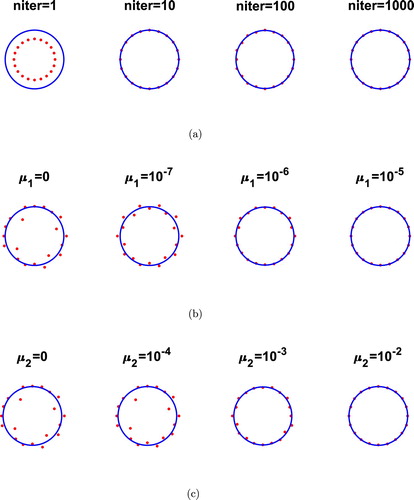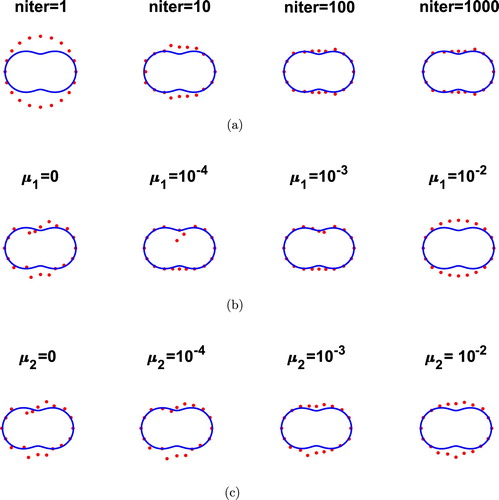and the initial guess a circle of radius 0.7. In Figure 3(a) we show the convergence of the numerical results for various numbers of iterations niter, no noise (p = 0) and no regularization (${\mu }_1={\mu }_2=0$), for inverse problem (1(1) $\begin{array}{rl}\mu \mathrm{\Delta }\mathit{u}-\mathrm{\nabla }p& =u_0\varrho \frac{\mathrm{\partial }\mathit{u}}{\mathrm{\partial }{x}_1}\text{in}\mathrm{\Omega }\mathrm{\setminus }\overline{D},\end{array}$(1) )–(5(5) $\begin{array}{rl}\mathit{t}& =\mathit{g}\text{on}\mathrm{\Gamma },\end{array}$(5) ). The results for p = 5% noise and various ${\mu }_1$ when ${\mu }_2=0$, and various ${\mu }_2$ when ${\mu }_1=0$, for niter =1000 are illustrated in Figure 3(b,c), respectively. These are showing the stable reconstructions obtained provided that regularization with a suitable parameter is employed.

Figure 3. Example 1: Reconstructions (a) with no noise and no regularization, (b) for various values of ${\mu }_1$ and ${\mu }_2=0$ for p = 5% noise, (c) for various values of ${\mu }_2$ and ${\mu }_1=0$ for $p=5$% noise, for inverse problem (1(1) $\begin{array}{rl}\mu \mathrm{\Delta }\mathit{u}-\mathrm{\nabla }p& =u_0\varrho \frac{\mathrm{\partial }\mathit{u}}{\mathrm{\partial }{x}_1}\text{in}\mathrm{\Omega }\mathrm{\setminus }\overline{D},\end{array}$(1) )–(5(5) $\begin{array}{rl}\mathit{t}& =\mathit{g}\text{on}\mathrm{\Gamma },\end{array}$(5) ).

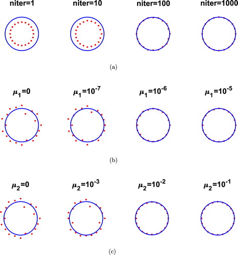
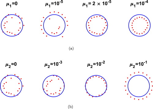
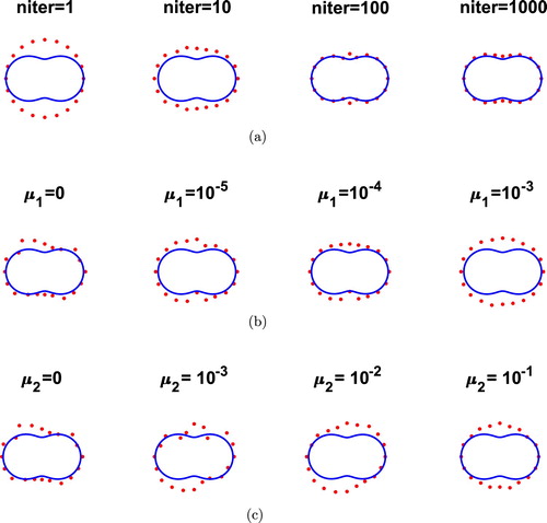
For inverse problem (1(1) $\begin{array}{rl}\mu \mathrm{\Delta }\mathit{u}-\mathrm{\nabla }p& =u_0\varrho \frac{\mathrm{\partial }\mathit{u}}{\mathrm{\partial }{x}_1}\text{in}\mathrm{\Omega }\mathrm{\setminus }\overline{D},\end{array}$(1) )–(4(4) $\begin{array}{rl}\mathit{u}& =\mathit{f}\text{on}\mathrm{\partial }\mathrm{\Omega },\end{array}$(4) ) and (6(6) $\mathrm{\nabla }p=\mathit{h}\text{on}\mathrm{\Gamma },$(6) ), the corresponding numerical reconstructions are illustrated in Figure 4 and the same conclusions as in Figure 3 can be observed. In some instances the method converges in fewer iterations than the prescribed number niter because the change in the sum of squares relative to its initial value is less than the selected value of the function tolerance.

Figure 4. Example 1: Reconstructions (a) with no noise and no regularization, (b) for various values of ${\mu }_1$ and ${\mu }_2=0$ for p = 5% noise, (c) for various values of ${\mu }_2$ and ${\mu }_1=0$ for $p=5$% noise, for inverse problem (1(1) $\begin{array}{rl}\mu \mathrm{\Delta }\mathit{u}-\mathrm{\nabla }p& =u_0\varrho \frac{\mathrm{\partial }\mathit{u}}{\mathrm{\partial }{x}_1}\text{in}\mathrm{\Omega }\mathrm{\setminus }\overline{D},\end{array}$(1) )–(4(4) $\begin{array}{rl}\mathit{u}& =\mathit{f}\text{on}\mathrm{\partial }\mathrm{\Omega },\end{array}$(4) ) and (6(6) $\mathrm{\nabla }p=\mathit{h}\text{on}\mathrm{\Gamma },$(6) ).

We have also considered the case of limited aperture data (5(5) $\begin{array}{rl}\mathit{t}& =\mathit{g}\text{on}\mathrm{\Gamma },\end{array}$(5) ) or (6(6) $\mathrm{\nabla }p=\mathit{h}\text{on}\mathrm{\Gamma },$(6) ) taken over an arc $\mathrm{\Gamma }\subset \mathrm{\partial }B(\mathbf{0};R)$. For p = 5% noise, the numerical reconstructions of the circular shape obstacle (29(29) $\mathrm{r}\left(\vartheta \right)=1,\vartheta \in [0,2\pi ).$(29) ) for the inverse problems (1(1) $\begin{array}{rl}\mu \mathrm{\Delta }\mathit{u}-\mathrm{\nabla }p& =u_0\varrho \frac{\mathrm{\partial }\mathit{u}}{\mathrm{\partial }{x}_1}\text{in}\mathrm{\Omega }\mathrm{\setminus }\overline{D},\end{array}$(1) )–(5(5) $\begin{array}{rl}\mathit{t}& =\mathit{g}\text{on}\mathrm{\Gamma },\end{array}$(5) ) and (1(1) $\begin{array}{rl}\mu \mathrm{\Delta }\mathit{u}-\mathrm{\nabla }p& =u_0\varrho \frac{\mathrm{\partial }\mathit{u}}{\mathrm{\partial }{x}_1}\text{in}\mathrm{\Omega }\mathrm{\setminus }\overline{D},\end{array}$(1) )–(4(4) $\begin{array}{rl}\mathit{u}& =\mathit{f}\text{on}\mathrm{\partial }\mathrm{\Omega },\end{array}$(4) ) and (6(6) $\mathrm{\nabla }p=\mathit{h}\text{on}\mathrm{\Gamma },$(6) ), and Γ is 2/3 or 1/3 of the exterior boundary $\mathrm{\partial }B(\mathbf{0};R)$, are illustrated, for various ${\mu }_1$ when ${\mu }_2=0$ and ${\mu }_2$ when ${\mu }_1=0$, in Figures 5 and 7, and 6 and 8, respectively. Although uniqueness of solution due to analytical continuation holds for any non-zero measure boundary Γ, we expect that the stability decreases as the length of Γ decreases. Consequently, as expected, compared to the case of full data (5(5) $\begin{array}{rl}\mathit{t}& =\mathit{g}\text{on}\mathrm{\Gamma },\end{array}$(5) ) or (6(6) $\mathrm{\nabla }p=\mathit{h}\text{on}\mathrm{\Gamma },$(6) ) on $\mathrm{\Gamma }=\mathrm{\partial }\mathrm{\Omega }=\mathrm{\partial }B(\mathbf{0};R)$ illustrated in Figures 3(b,c) and 4(b,c), it can be seen that, in the limited aperture case, the results become more sensitive to the choice of the regularization parameter ${\mu }_1$ or ${\mu }_2$, but still stable and accurate reconstructions can be observed. The more ill-posed case of supplying the potential boundary velocity data (8(8) $\mathit{u}=\mathit{f}\text{on}\mathrm{\Gamma }.$(8) ) on Γ instead of the full data (4(4) $\begin{array}{rl}\mathit{u}& =\mathit{f}\text{on}\mathrm{\partial }\mathrm{\Omega },\end{array}$(4) ) on $\mathrm{\partial }\mathrm{\Omega }$ can also be considered.

Figure 5. Example 1, aperture case, Γ is 2/3 of the exterior circle: Reconstructions with $p=5$% noise, (a) for various values of ${\mu }_1$ and ${\mu }_2=0$, (b) for various values of ${\mu }_2$ and ${\mu }_1=0$, for inverse problem (1(1) $\begin{array}{rl}\mu \mathrm{\Delta }\mathit{u}-\mathrm{\nabla }p& =u_0\varrho \frac{\mathrm{\partial }\mathit{u}}{\mathrm{\partial }{x}_1}\text{in}\mathrm{\Omega }\mathrm{\setminus }\overline{D},\end{array}$(1) )–(5(5) $\begin{array}{rl}\mathit{t}& =\mathit{g}\text{on}\mathrm{\Gamma },\end{array}$(5) ).

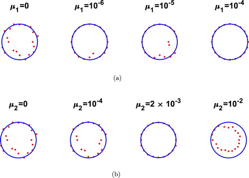
Figure 6. Example 1, aperture case, Γ is 2/3 of the exterior circle: Reconstructions with $p=5$% noise, (a) for various values of ${\mu }_1$ and ${\mu }_2=0$, (b) for various values of ${\mu }_2$ and ${\mu }_1=0$, for inverse problem (1(1) $\begin{array}{rl}\mu \mathrm{\Delta }\mathit{u}-\mathrm{\nabla }p& =u_0\varrho \frac{\mathrm{\partial }\mathit{u}}{\mathrm{\partial }{x}_1}\text{in}\mathrm{\Omega }\mathrm{\setminus }\overline{D},\end{array}$(1) )–(4(4) $\begin{array}{rl}\mathit{u}& =\mathit{f}\text{on}\mathrm{\partial }\mathrm{\Omega },\end{array}$(4) ) and (6(6) $\mathrm{\nabla }p=\mathit{h}\text{on}\mathrm{\Gamma },$(6) ).

Figure 7. Example 1, aperture case, Γ is 1/3 of the exterior circle: Reconstructions with $p=5$% noise, (a) for various values of ${\mu }_1$ and ${\mu }_2=0$, (b) for various values of ${\mu }_2$ and ${\mu }_1=0$, for inverse problem (1(1) $\begin{array}{rl}\mu \mathrm{\Delta }\mathit{u}-\mathrm{\nabla }p& =u_0\varrho \frac{\mathrm{\partial }\mathit{u}}{\mathrm{\partial }{x}_1}\text{in}\mathrm{\Omega }\mathrm{\setminus }\overline{D},\end{array}$(1) )–(5(5) $\begin{array}{rl}\mathit{t}& =\mathit{g}\text{on}\mathrm{\Gamma },\end{array}$(5) ).

Figure 8. Example 1, aperture case, Γ is 1/3 of the exterior circle: Reconstructions with $p=5$% noise, (a) for various values of ${\mu }_1$ and ${\mu }_2=0$, (b) for various values of ${\mu }_2$ and ${\mu }_1=0$, for inverse problem (1(1) $\begin{array}{rl}\mu \mathrm{\Delta }\mathit{u}-\mathrm{\nabla }p& =u_0\varrho \frac{\mathrm{\partial }\mathit{u}}{\mathrm{\partial }{x}_1}\text{in}\mathrm{\Omega }\mathrm{\setminus }\overline{D},\end{array}$(1) )–(4(4) $\begin{array}{rl}\mathit{u}& =\mathit{f}\text{on}\mathrm{\partial }\mathrm{\Omega },\end{array}$(4) ) and (6(6) $\mathrm{\nabla }p=\mathit{h}\text{on}\mathrm{\Gamma },$(6) ).

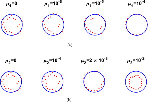
4.2. Example 2: peanut-shaped obstacle

We attempt to reconstruct a more irregular shape than the previous example, given by a peanut-shaped obstacle D with the parametrization [4, 6, 16] (30) $r\left(\vartheta \right)=\frac{1}{2}\sqrt{1+3{\cos }^2\left(\vartheta \right)},\vartheta \in [0,2\pi ).$(30) The direct problem (1(1) $\begin{array}{rl}\mu \mathrm{\Delta }\mathit{u}-\mathrm{\nabla }p& =u_0\varrho \frac{\mathrm{\partial }\mathit{u}}{\mathrm{\partial }{x}_1}\text{in}\mathrm{\Omega }\mathrm{\setminus }\overline{D},\end{array}$(1) )–(4(4) $\begin{array}{rl}\mathit{u}& =\mathit{f}\text{on}\mathrm{\partial }\mathrm{\Omega },\end{array}$(4) ) was solved with $M=60,N=30$ and ${\eta }_{\mathrm{i}\mathrm{n}\mathrm{t}}=0.95$ and ${\eta }_{\mathrm{e}\mathrm{x}\mathrm{t}}=5/3$. We took $r_{\mathrm{m}\mathrm{i}\mathrm{n}}=0.1$ and $r_{\mathrm{m}\mathrm{a}\mathrm{x}}=1.5$ and the initial guess a circle of radius 1. The inputs (27(27) $\mathit{u}(x,y)=\mathit{f}(x,y)=(-y,x),(x,y)\in \mathrm{\partial }\mathrm{\Omega },$(27) ) and (28(28) ${\mathit{g}}^{\epsilon }\left({\mathit{x}}_k\right)=(1+{\chi }_k\mathrm{p})\mathit{g}\left({\mathit{x}}_k\right),{\mathit{h}}^{\epsilon }\left({\mathit{x}}_k\right)=(1+{\chi }_k\mathrm{p})\mathit{h}\left({\mathit{x}}_k\right),k=\overline{1,M_1},$(28) ), and the remaining computational details for the inverse problems are the same as in the previous example. Figures 9 and 10 represent the same quantities as Figures 3 and 4 but with p = 3% noise, respectively, and the same performant reconstructions in terms of accuracy and stability can be observed. Also, on comparing Figures 9(b) and 10(b) with Figures 9(c) and 10(c) it can be seen that regularization with ${\mu }_1>0$ is more stable and accurate than regularization with ${\mu }_2>0$. Based on (20(20) $\mathcal{R}(\mathit{\alpha },\text{β},\mathrm{\nabla }\mathrm{r};{\mu }_1,{\mu }_2)={\mu }_1\left(|\mathit{\alpha }{|}^2+|\text{β}{|}^2\right)+{\mu }_2\parallel \mathrm{\nabla }\mathrm{r}{\parallel }_{L^2\left(\mathrm{\partial }D\right)}^2,$(20) ) or (25(25) $\mathcal{R}(\mathit{\alpha },\text{β},{\mathbf{r}}^{\mathrm{\prime }};{\mu }_1,{\mu }_2)={\mu }_1\left(|\mathit{\alpha }{|}^2+|\text{β}{|}^2\right)+{\mu }_2\sum _{j=2}^N{\left({\mathrm{r}}_j-{\mathrm{r}}_{j-1}\right)}^2,$(25) ), that is, penalizing the MFS coefficients $\mathit{\alpha }$ and $\text{β}$ is more important to alleviate the ill-conditioning than penalizing the shape $\mathbf{r}$ dealing with the smoothness and nonlinearity of the obstacle. One can also consider allowing at the same time both positive regularization parameters ${\mu }_1$ and ${\mu }_2$, but the investigation becomes more tedious. Finally, on comparing Figures 9 and 10 it appears that the stress force measurement (5(5) $\begin{array}{rl}\mathit{t}& =\mathit{g}\text{on}\mathrm{\Gamma },\end{array}$(5) ) contains more information than the pressure gradient measurement (6(6) $\mathrm{\nabla }p=\mathit{h}\text{on}\mathrm{\Gamma },$(6) ).

Figure 9. Example 2: Reconstructions (a) with no noise and no regularization, (b) for various values of ${\mu }_1$ and ${\mu }_2=0$ for p = 3% noise, (c) for various values of ${\mu }_2$ and ${\mu }_1=0$ for $p=3$% noise, for inverse problem (1(1) $\begin{array}{rl}\mu \mathrm{\Delta }\mathit{u}-\mathrm{\nabla }p& =u_0\varrho \frac{\mathrm{\partial }\mathit{u}}{\mathrm{\partial }{x}_1}\text{in}\mathrm{\Omega }\mathrm{\setminus }\overline{D},\end{array}$(1) )–(5(5) $\begin{array}{rl}\mathit{t}& =\mathit{g}\text{on}\mathrm{\Gamma },\end{array}$(5) ).

Figure 10. Example 2: Reconstructions (a) with no noise and no regularization, (b) for various values of ${\mu }_1$ and ${\mu }_2=0$ for p = 3% noise, (c) for various values of ${\mu }_2$ and ${\mu }_1=0$ for $p=3$% noise, for inverse problem (1(1) $\begin{array}{rl}\mu \mathrm{\Delta }\mathit{u}-\mathrm{\nabla }p& =u_0\varrho \frac{\mathrm{\partial }\mathit{u}}{\mathrm{\partial }{x}_1}\text{in}\mathrm{\Omega }\mathrm{\setminus }\overline{D},\end{array}$(1) )–(4(4) $\begin{array}{rl}\mathit{u}& =\mathit{f}\text{on}\mathrm{\partial }\mathrm{\Omega },\end{array}$(4) ) and (6(6) $\mathrm{\nabla }p=\mathit{h}\text{on}\mathrm{\Gamma },$(6) ).

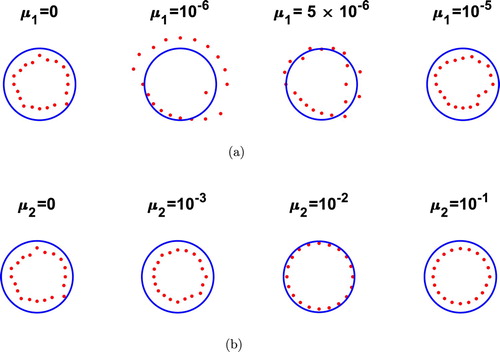
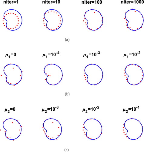
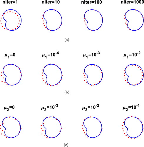
4.3. Example 3: bean-shaped obstacle

We attempt to reconstruct a more irregular shape than the previous example, given by a bean-shaped obstacle D with the parametrization [4, 6, 7] (31) $r\left(\vartheta \right)=\frac{1+0.9\cos \left(\vartheta \right)+0.1\sin \left(\vartheta \right)}{1+0.75\cos \left(\vartheta \right)},\vartheta \in [0,2\pi ).$(31) The direct problem (1(1) $\begin{array}{rl}\mu \mathrm{\Delta }\mathit{u}-\mathrm{\nabla }p& =u_0\varrho \frac{\mathrm{\partial }\mathit{u}}{\mathrm{\partial }{x}_1}\text{in}\mathrm{\Omega }\mathrm{\setminus }\overline{D},\end{array}$(1) )–(4(4) $\begin{array}{rl}\mathit{u}& =\mathit{f}\text{on}\mathrm{\partial }\mathrm{\Omega },\end{array}$(4) ) was solved with $M=60,N=30$ and ${\eta }_{\mathrm{i}\mathrm{n}\mathrm{t}}=0.95$ and ${\eta }_{\mathrm{e}\mathrm{x}\mathrm{t}}=5/3$. We took $r_{\mathrm{m}\mathrm{i}\mathrm{n}}=0.1$ and $r_{\mathrm{m}\mathrm{a}\mathrm{x}}=1.5$ and the initial guess a circle of radius 0.75 for problem (1(1) $\begin{array}{rl}\mu \mathrm{\Delta }\mathit{u}-\mathrm{\nabla }p& =u_0\varrho \frac{\mathrm{\partial }\mathit{u}}{\mathrm{\partial }{x}_1}\text{in}\mathrm{\Omega }\mathrm{\setminus }\overline{D},\end{array}$(1) )–(5(5) $\begin{array}{rl}\mathit{t}& =\mathit{g}\text{on}\mathrm{\Gamma },\end{array}$(5) ) and radius 0.9 for problem (1(1) $\begin{array}{rl}\mu \mathrm{\Delta }\mathit{u}-\mathrm{\nabla }p& =u_0\varrho \frac{\mathrm{\partial }\mathit{u}}{\mathrm{\partial }{x}_1}\text{in}\mathrm{\Omega }\mathrm{\setminus }\overline{D},\end{array}$(1) )–(4(4) $\begin{array}{rl}\mathit{u}& =\mathit{f}\text{on}\mathrm{\partial }\mathrm{\Omega },\end{array}$(4) ) and (6(6) $\mathrm{\nabla }p=\mathit{h}\text{on}\mathrm{\Gamma },$(6) ). The inputs (27(27) $\mathit{u}(x,y)=\mathit{f}(x,y)=(-y,x),(x,y)\in \mathrm{\partial }\mathrm{\Omega },$(27) ) and (28(28) ${\mathit{g}}^{\epsilon }\left({\mathit{x}}_k\right)=(1+{\chi }_k\mathrm{p})\mathit{g}\left({\mathit{x}}_k\right),{\mathit{h}}^{\epsilon }\left({\mathit{x}}_k\right)=(1+{\chi }_k\mathrm{p})\mathit{h}\left({\mathit{x}}_k\right),k=\overline{1,M_1},$(28) ), and the remaining computational details for both the direct and the inverse problems are the same as in the previous example. Figures 11 and 12 represent the same quantities as Figures 9 and 10, respectively, and the same conclusions on the good reconstructions in terms of accuracy and stability can be observed.

Figure 11. Example 3: Reconstructions (a) with no noise and no regularization, (b) for various values of ${\mu }_1$ and ${\mu }_2=0$ for p = 3% noise, (c) for various values of ${\mu }_2$ and ${\mu }_1=0$ for $p=3$% noise, for inverse problem (1(1) $\begin{array}{rl}\mu \mathrm{\Delta }\mathit{u}-\mathrm{\nabla }p& =u_0\varrho \frac{\mathrm{\partial }\mathit{u}}{\mathrm{\partial }{x}_1}\text{in}\mathrm{\Omega }\mathrm{\setminus }\overline{D},\end{array}$(1) )–(5(5) $\begin{array}{rl}\mathit{t}& =\mathit{g}\text{on}\mathrm{\Gamma },\end{array}$(5) ).

Figure 12. Example 3: Reconstructions (a) with no noise and no regularization, (b) for various values of ${\mu }_1$ and ${\mu }_2=0$ for p = 3% noise, (c) for various values of ${\mu }_2$ and ${\mu }_1=0$ for $p=3$% noise, for inverse problem (1(1) $\begin{array}{rl}\mu \mathrm{\Delta }\mathit{u}-\mathrm{\nabla }p& =u_0\varrho \frac{\mathrm{\partial }\mathit{u}}{\mathrm{\partial }{x}_1}\text{in}\mathrm{\Omega }\mathrm{\setminus }\overline{D},\end{array}$(1) )–(4(4) $\begin{array}{rl}\mathit{u}& =\mathit{f}\text{on}\mathrm{\partial }\mathrm{\Omega },\end{array}$(4) ) and (6(6) $\mathrm{\nabla }p=\mathit{h}\text{on}\mathrm{\Gamma },$(6) ).

5. Conclusions

In this paper, the reconstruction of interior obstacles immersed in a stationary incompressible Oseen fluid from exterior boundary measurements of the fluid velocity, stress force or the pressure gradient has been considered. The approximations of the fluid velocity and pressure are based on the MFS finite sums (9(9) $\begin{array}{rl}{u}_i\left(\mathit{x}\right)& =\sum _{j=1}^{M+N}\left({\alpha }_j{U}_{i1}(\mathit{x},{\mathit{\xi }}_j)+{\text{β}}_j{U}_{i2}(\mathit{x},{\mathit{\xi }}_j)\right),i=1,2,\mathit{x}\in \overline{\mathrm{\Omega }}\mathrm{\setminus }D,\end{array}$(9) ) and (10(10) $\begin{array}{rl}p\left(\mathit{x}\right)& =\sum _{j=1}^{M+N}\left({\alpha }_j{P}_1(\mathit{x},{\mathit{\xi }}_j)+{\text{β}}_j{P}_2(\mathit{x},{\mathit{\xi }}_j)\right),i=1,2,\mathit{x}\in \overline{\mathrm{\Omega }}\mathrm{\setminus }D,\end{array}$(10) ). The nonlinear objective functions (22(22) $\begin{array}{rl}{\mathcal{F}}_1(\mathit{\alpha },\text{β},\mathbf{r},{\eta }_{\mathrm{i}\mathrm{n}\mathrm{t}},{\eta }_{\mathrm{e}\mathrm{x}\mathrm{t}})& =T_0(\mathit{\alpha },\text{β},\mathbf{r},{\eta }_{\mathrm{i}\mathrm{n}\mathrm{t}},{\eta }_{\mathrm{e}\mathrm{x}\mathrm{t}})+T_{\mathit{f}}(\mathit{\alpha },\text{β},\mathbf{r},{\eta }_{\mathrm{i}\mathrm{n}\mathrm{t}},{\eta }_{\mathrm{e}\mathrm{x}\mathrm{t}})\\ & +T_{{\mathit{g}}^{\epsilon }}(\mathit{\alpha },\text{β},\mathbf{r},{\eta }_{\mathrm{i}\mathrm{n}\mathrm{t}},{\eta }_{\mathrm{e}\mathrm{x}\mathrm{t}})+\mathcal{R}(\mathit{\alpha },\text{β},{\mathbf{r}}^{\mathrm{\prime }};{\mu }_1,{\mu }_2),\end{array}$(22) )–(24(24) $\begin{array}{rl}{\mathcal{F}}_3(\mathit{\alpha },\text{β},\mathbf{r},{\eta }_{\mathrm{i}\mathrm{n}\mathrm{t}},{\eta }_{\mathrm{e}\mathrm{x}\mathrm{t}})& =T_0(\mathit{\alpha },\text{β},\mathbf{r},{\eta }_{\mathrm{i}\mathrm{n}\mathrm{t}},{\eta }_{\mathrm{e}\mathrm{x}\mathrm{t}})+T_{\mathit{f}}^1(\mathit{\alpha },\text{β},\mathbf{r},{\eta }_{\mathrm{i}\mathrm{n}\mathrm{t}},{\eta }_{\mathrm{e}\mathrm{x}\mathrm{t}})\\ & +T_{{\mathit{g}}^{\epsilon }}(\mathit{\alpha },\text{β},\mathbf{r},{\eta }_{\mathrm{i}\mathrm{n}\mathrm{t}},{\eta }_{\mathrm{e}\mathrm{x}\mathrm{t}})+\mathcal{R}(\mathit{\alpha },\text{β},{\mathbf{r}}^{\mathrm{\prime }};{\mu }_1,{\mu }_2),\end{array}$(24) ) have been minimized with respect to the MFS characteristics $\mathit{\alpha },\text{β},{\eta }_{\mathrm{i}\mathrm{n}\mathrm{t}}$ and ${\eta }_{\mathrm{e}\mathrm{x}\mathrm{t}}$, and the polar radius $\mathrm{r}\left(\vartheta \right)$ parameterizing the star-shaped obstacle (11(11) $D:=\left\{\mathrm{r}\left(\vartheta \right)\left(\cos \vartheta ,\sin \vartheta \right)|\vartheta \in [0,2\pi )\right\},\text{where}0<\mathrm{r}\left(\vartheta \right)<R,$(11) ), subject to the constraints (26(26) $\begin{array}{rl}-{10}^5& \le {\alpha }_j\le {10}^5,-{10}^5\le {\text{β}}_j\le {10}^5,j=\overline{1,M+N},\\ 0& <{\mathrm{r}}_{\mathrm{m}\mathrm{i}\mathrm{n}}\le {\mathrm{r}}_{\ell }\le {\mathrm{r}}_{\mathrm{m}\mathrm{a}\mathrm{x}}<R,\ell =\overline{1,N},\\ 0.1& \le {\eta }_{\mathrm{i}\mathrm{n}\mathrm{t}}\le 0.99,1.1\le {\eta }_{\mathrm{e}\mathrm{x}\mathrm{t}}\le 2,\end{array}$(26) ) using the MATLAB${}^{\copyright }$ toolbox routine lsqnonlin. The numerical results show accurate and stable reconstructions provided that regularization is included, especially in penalizing the MFS coefficients problem (1(1) $\begin{array}{rl}\mu \mathrm{\Delta }\mathit{u}-\mathrm{\nabla }p& =u_0\varrho \frac{\mathrm{\partial }\mathit{u}}{\mathrm{\partial }{x}_1}\text{in}\mathrm{\Omega }\mathrm{\setminus }\overline{D},\end{array}$(1) )–(5(5) $\begin{array}{rl}\mathit{t}& =\mathit{g}\text{on}\mathrm{\Gamma },\end{array}$(5) ). Also, it seems that the stress force measurements (5(5) $\begin{array}{rl}\mathit{t}& =\mathit{g}\text{on}\mathrm{\Gamma },\end{array}$(5) ) contain more information than the pressure gradient measurements (6(6) $\mathrm{\nabla }p=\mathit{h}\text{on}\mathrm{\Gamma },$(6) ). The MFS has further potential for extensions to three-dimensional such Oseen obstacle problems.

Acknowledgments

The authors are grateful to the University of Cyprus for supporting this research.

Disclosure statement

No potential conflict of interest was reported by the authors.

Appendix

In this appendix we provide the formulæ for the partial derivatives needed for expressing the stress force (5(5) $\begin{array}{rl}\mathit{t}& =\mathit{g}\text{on}\mathrm{\Gamma },\end{array}$(5) ) and the pressure gradient (6(6) $\mathrm{\nabla }p=\mathit{h}\text{on}\mathrm{\Gamma },$(6) ). (A1) $\mathrm{\nabla }p\left(\mathit{x}\right)=\sum _{j=1}^{M+N}\left({\alpha }_j\mathrm{\nabla }{P}_1(\mathit{x},{\mathit{\xi }}_j)+{\text{β}}_j\mathrm{\nabla }{P}_2(\mathit{x},{\mathit{\xi }}_j)\right),$(A1) where $\begin{array}{rl}\mathrm{\nabla }{P}_1(\mathit{x},{\mathit{x}}^{\mathrm{\prime }})& =\left(\frac{\mathrm{\partial }{P}_1}{\mathrm{\partial }x},\frac{\mathrm{\partial }{P}_1}{\mathrm{\partial }y}\right)=\left(\frac{(y-y^{\mathrm{\prime }}{)}^2-(x-x^{\mathrm{\prime }}{)}^2}{r^4},-\frac{2(x-x^{\mathrm{\prime }})(y-y^{\mathrm{\prime }})}{r^4}\right),\\ \mathrm{\nabla }{P}_2(\mathit{x},{\mathit{x}}^{\mathrm{\prime }})& =\left(\frac{\mathrm{\partial }{P}_2}{\mathrm{\partial }x},\frac{\mathrm{\partial }{P}_2}{\mathrm{\partial }y}\right)=\left(-\frac{2(x-x^{\mathrm{\prime }})(y-y^{\mathrm{\prime }})}{r^4},\frac{(x-x^{\mathrm{\prime }}{)}^2-(y-y^{\mathrm{\prime }}{)}^2}{r^4}\right),\\ \frac{\mathrm{\partial }{U}_{11}}{\mathrm{\partial }x}(\mathit{x},{\mathit{x}}^{\mathrm{\prime }})& ={\kappa }^2{\mathrm{e}}^{\kappa (x-x^{\mathrm{\prime }})}\left[1-\frac{(x-x^{\mathrm{\prime }}{)}^2}{2r^2}\right]K_0\left(\kappa r\right)+\kappa {\mathrm{e}}^{\kappa (x-x^{\mathrm{\prime }})}\frac{(y-y^{\mathrm{\prime }}{)}^2}{r^3}{K}_1\left(\kappa r\right)\\ & -{\kappa }^2{\mathrm{e}}^{\kappa (x-x^{\mathrm{\prime }})}\frac{(x-x^{\mathrm{\prime }}{)}^2}{2r^2}{K}_2\left(\kappa r\right)+\frac{(x-x^{\mathrm{\prime }}{)}^2-(y-y^{\mathrm{\prime }}{)}^2}{r^4},\\ \frac{\mathrm{\partial }{U}_{11}}{\mathrm{\partial }y}(\mathit{x},{\mathit{x}}^{\mathrm{\prime }})& =-{\kappa }^2{\mathrm{e}}^{\kappa (x-x^{\mathrm{\prime }})}\frac{(x-x^{\mathrm{\prime }})(y-y^{\mathrm{\prime }})}{2r^2}{K}_0\left(\kappa r\right)-\kappa {\mathrm{e}}^{\kappa (x-x^{\mathrm{\prime }})}\frac{(y-y^{\mathrm{\prime }})}{r}\left[\kappa +\frac{(x-x^{\mathrm{\prime }})}{r^2}\right]K_1\left(\kappa r\right)\\ & -{\kappa }^2{\mathrm{e}}^{\kappa (x-x^{\mathrm{\prime }})}\frac{(x-x^{\mathrm{\prime }})(y-y^{\mathrm{\prime }})}{2r^2}{K}_2\left(\kappa r\right)+\frac{2(x-x^{\mathrm{\prime }})(y-y^{\mathrm{\prime }})}{r^4},\\ \frac{\mathrm{\partial }{U}_{22}}{\mathrm{\partial }x}(\mathit{x},{\mathit{x}}^{\mathrm{\prime }})& =\frac{(y-y^{\mathrm{\prime }}{)}^2-(x-x^{\mathrm{\prime }}{)}^2}{r^4}+{\kappa }^2{\mathrm{e}}^{\kappa (x-x^{\mathrm{\prime }})}\left[1+\frac{(x-x^{\mathrm{\prime }}{)}^2}{2r^2}\right]K_0\left(\kappa r\right)\\ & -\kappa {\mathrm{e}}^{\kappa (x-x^{\mathrm{\prime }})}\left[\frac{2\kappa (x-x^{\mathrm{\prime }})}{r}+\frac{(y-y^{\mathrm{\prime }}{)}^2}{r^3}\right]K_1\left(\kappa r\right)+{\kappa }^2{\mathrm{e}}^{\kappa (x-x^{\mathrm{\prime }})}\frac{(x-x^{\mathrm{\prime }}{)}^2}{2r^2}{K}_2\left(\kappa r\right),\\ \frac{\mathrm{\partial }{U}_{22}}{\mathrm{\partial }y}(\mathit{x},{\mathit{x}}^{\mathrm{\prime }})& =-\frac{2(x-x^{\mathrm{\prime }})(y-y^{\mathrm{\prime }})}{r^4}+{\kappa }^2{\mathrm{e}}^{\kappa (x-x^{\mathrm{\prime }})}\frac{(x-x^{\mathrm{\prime }})(y-y^{\mathrm{\prime }})}{2r^2}{K}_0\left(\kappa r\right)\\ & +\kappa {\mathrm{e}}^{\kappa (x-x^{\mathrm{\prime }})}\frac{(y-y^{\mathrm{\prime }})}{r}\left[-\kappa +\frac{(x-x^{\mathrm{\prime }})}{r^2}\right]K_1\left(\kappa r\right)+{\kappa }^2{\mathrm{e}}^{\kappa (x-x^{\mathrm{\prime }})}\frac{(x-x^{\mathrm{\prime }})(y-y^{\mathrm{\prime }})}{2r^2}{K}_2\left(\kappa r\right),\\ \frac{\mathrm{\partial }{U}_{12}}{\mathrm{\partial }x}(\mathit{x},{\mathit{x}}^{\mathrm{\prime }})& =\frac{\mathrm{\partial }{U}_{21}}{\mathrm{\partial }x}(\mathit{x},{\mathit{x}}^{\mathrm{\prime }})=\frac{2(x-x^{\mathrm{\prime }})(y-y^{\mathrm{\prime }})}{r^4}-{\kappa }^2{\mathrm{e}}^{\kappa (x-x^{\mathrm{\prime }})}\frac{(x-x^{\mathrm{\prime }})(y-y^{\mathrm{\prime }})}{2r^2}{K}_0\left(\kappa r\right)\\ & +\kappa {\mathrm{e}}^{\kappa (x-x^{\mathrm{\prime }})}\frac{(y-y^{\mathrm{\prime }})}{r}\left[\kappa -\frac{(x-x^{\mathrm{\prime }})}{r^2}\right]K_1\left(\kappa r\right)-{\kappa }^2{\mathrm{e}}^{\kappa (x-x^{\mathrm{\prime }})}\frac{(x-x^{\mathrm{\prime }})(y-y^{\mathrm{\prime }})}{2r^2}{K}_2\left(\kappa r\right),\\ \frac{\mathrm{\partial }{U}_{12}}{\mathrm{\partial }y}(\mathit{x},{\mathit{x}}^{\mathrm{\prime }})& =\frac{\mathrm{\partial }{U}_{21}}{\mathrm{\partial }y}(\mathit{x},{\mathit{x}}^{\mathrm{\prime }})=\frac{(y-y^{\mathrm{\prime }}{)}^2-(x-x^{\mathrm{\prime }}{)}^2}{r^4}-{\kappa }^2{\mathrm{e}}^{\kappa (x-x^{\mathrm{\prime }})}\frac{(y-y^{\mathrm{\prime }}{)}^2}{2r^2}{K}_0\left(\kappa r\right)\\ & +\kappa {\mathrm{e}}^{\kappa (x-x^{\mathrm{\prime }})}\frac{(x-x^{\mathrm{\prime }}{)}^2}{r^3}{K}_1\left(\kappa r\right)-{\kappa }^2{\mathrm{e}}^{\kappa (x-x^{\mathrm{\prime }})}\frac{(y-y^{\mathrm{\prime }}{)}^2}{2r^2}{K}_2\left(\kappa r\right).\end{array}$ In the derivation of the above expressions, we have used the identities $K_0^{\mathrm{\prime }}\left(s\right)=-K_1\left(s\right),K_1^{\mathrm{\prime }}\left(s\right)=-\frac{1}{2}\left(K_0\left(s\right)+K_2\left(s\right)\right),$ where $K_2$ is the modified Bessel function of the second kind of order two.

References

- Conca C, Cumsille P, Ortega J, et al. On the detection of a moving obstacle in an ideal fluid by a boundary measurement. Inverse Probl. 2008;24:045001 (18 pp). doi: 10.1088/0266-5611/24/4/045001
- Alves CJS, Kress R, Silvestre AL. Integral equations for an inverse boundary value problem for the two-dimensional Stokes equations. J Inverse Ill-Posed Probl. 2007;15:461–481. doi: 10.1515/jiip.2007.026
- Alvarez C, Conca C, Friz L, et al. Identification of immersed obstacles via boundary measurements. Inverse Probl. 2005;21:1531–1552. doi: 10.1088/0266-5611/21/5/003
- Karageorghis A, Lesnic D. The method of fundamental solutions for the Oseen steady-state viscous flow past obstacles of known or unknown shapes. Numer Methods Partial Diff Eq. 2019;35:2103–2119. doi: 10.1002/num.22404
- Karageorghis A, Lesnic D, Marin L. A survey of applications of the MFS to inverse problems. Inverse Probl Sci Eng. 2011;19:309–336. doi: 10.1080/17415977.2011.551830
- Kress R, Meyer S. An inverse boundary value problem for the Oseen equation. Math Meth Appl Sci. 2000;23:103–120. doi: 10.1002/(SICI)1099-1476(20000125)23:2<103::AID-MMA106>3.0.CO;2-4
- Ballerini A. Stable determination of an immersed body in a stationary Stokes fluid. Inverse Probl. 2010;26:125015 (25 pp). doi: 10.1088/0266-5611/26/12/125015
- Bourgeois L, Dardé J. The ‘exterior approach’ to solve the inverse obstacle problem for the Stokes system. Inverse Probl Imaging. 2014;8:23–51. doi: 10.3934/ipi.2014.8.23
- Ballerini A. Stable determination of a body immersed in a fluid: the nonlinear stationary case. Appl Anal. 2013;92:460–481. doi: 10.1080/00036811.2011.628173
- Doubova A, Fernández-Cara AE, Ortega JH. On the identification of a single body immersed in a Navier-Stokes fluid. European J Appl Math. 2007;18:57–80. doi: 10.1017/S0956792507006821
- Fabre C, Lebeau G. Prolongement unique des solutions de l'équation de Stokes. Comm Partial Diff Eq. 1996;21:573–596. doi: 10.1080/03605309608821198
- Belge M, Kilmer M, Miller EL. Efficient determination of multiple regularization parameters in a generalized L-curve framework. Inverse Probl. 2002;18:1161–1183. doi: 10.1088/0266-5611/18/4/314
- Karageorghis A, Lesnic D. Application of the MFS to inverse obstacle scattering problems. Eng Anal Bound Elem. 2011;35:631–638. doi: 10.1016/j.enganabound.2010.11.010
- Lu S, Pereverzev SV. Multi-parameter regularization and its numerical realization. Numer Math. 2011;118:1–31. doi: 10.1007/s00211-010-0318-3
- The MathWorks, Inc., 3 Apple Hill Dr., Natick, MA, Matlab.
- Ivanyshyn O. Shape reconstruction of acoustic obstacles from the modulus of the far field pattern. Inverse Probl Imaging. 2007;1:609–622. doi: 10.3934/ipi.2007.1.609