A new method based on polynomials equipped with a parameter to solve two parabolic inverse problems with a nonlocal boundary condition

ABSTRACT

In this paper, a new method is used based on polynomials equipped with a parameter to solve two parabolic inverse problems. These inverse problems have nonlocal boundary conditions and over-determination of data that make it difficult to solve these problems. In this method, we use the combination of the finite difference method and the finite element method. In each point $t_j$, a nonlinear equation system is solved via the least-squares method, and then, we obtain an approximate function for the solution of the problem by using the interpolation of these points.

KEYWORDS:

• Inverse problem
• nonlocal boundary condition
• time-dependent diffusion coefficient
• collocation method
• source problem

2010 MATHEMATICS SUBJECT CLASSIFICATIONS:

• 65M32
• 35C11

1. Introduction

Today, inverse problems are very much applicable in engineering and physics branches such as optic [1], radar [2], acoustics [3], communication theory, signal processing [4], tomography, and medical imaging [5]. In particular, inverse problems of parameter identification are applied in image inpainting [6], heat conduction, microwave heating, and electromagnetic field [7]. There are different methods to solve inverse problems: Bernstein Galerkin method [8], finite difference method [9], regularization method, mollification method [10], radial basis function method [11], and reproducing kernel space method [12]. In this paper, a new method is proposed for the numerical solution of inverse problems to find the source parameter or control parameter in parabolic equations. Many methods are presented in various papers for the numerical solution of these inverse problems. In [13], a finite difference method was used to solve this problem. In [14], the problem is converted to a simpler problem with a variable change and then solved by a finite difference method. In [15], a method similar to [13] is used. In this problem, we face the nonlocal boundary conditions and over-determination of data, approximated in the above-mentioned papers by the method of finite difference. In [16], these inverse problems are solved by the method of reproducing kernel Hilbert space(RKHS).

In this paper, we will deal with two types of inverse problems as follows.

Problem 1: Finding a pair of functions $\{v(x,t),r(t)\}$ in the parabolic equation (1) $v_t-v_{xx}=r(t)v+f(x,t),(x,t)\in \mathrm{\Omega }=(0,1)\times [0,T],$(1) with the initial condition $v(x,0)=\phi (x),x\in [0,1],$ nonlocal boundary conditions $v(0,t)=v(1,t),v_x(1,t)=0,t\in [0,T],$ and the integral over-specified condition ${\int }_0^{1}v(x,t)\mathrm{d}x=E(t),t\in [0,T],$ where $f(x,t)$, $\phi (x)$ and $E(t)$ are known functions. The existence, uniqueness, and continuous dependence of the solution upon the data for this problem are demonstrated in [17].

Problem 2: Finding a pair of functions $\{v(x,t),p(t)\}$ in the parabolic equation (2) $v_t-v_{xx}=p(t)v+f(x,t),(x,t)\in \mathrm{\Omega }=(0,1)\times [0,T],$(2) with the initial condition $v(x,0)=\phi (x),x\in [0,1],$ nonlocal boundary conditions $v(0,t)=v(1,t),v_x(1,t)=0,t\in [0,T],$ and the over-specified condition at a point in the spatial domain $v(x^{\ast },t)=E(t),t\in [0,T],$ where $f(x,t)$, $\phi (x)$ and $E(t)$ are known functions. The existence, uniqueness, and continuous dependence of the solution upon the data for this problem are demonstrated in [14].

1.1. Existence, uniqueness, and continuous dependence of the solution

• Problem 1: Let us consider $\begin{array}{rl}& u_t=u_{xx}-a(t)u-F(x,t),Q_T=\left\{(x,t):0<x<1,0<t⩽T\right\},\\ & u(x,0)=\phi (x),0⩽x⩽1,\\ & u(0,t)=u(1,t),u_x(1,t)=0,0⩽t⩽T,\\ & {\int }_0^{1}u(x,t)\mathrm{d}x=E(t),0⩽t⩽T,\end{array}$ with the following assumptions:

  1. $\begin{array}{rl}& \phi (x)\in C^4[0,1],\\ & \phi (0)=\phi (1),{\phi }^{\prime }(1)=0,{\phi }^{″}(0)={\phi }^{″}(1),\\ & {\phi }_{2k}⩽0,k=1,2,\dots ;\end{array}$

  2. $\begin{array}{rl}& E(t)\in C^1[0,T],\\ & E(0)={\int }_0^1\phi (x)\mathrm{d}x,\\ & E(t)>0,E^{\prime }(t)⩽0,\mathrm{\forall }t\in [0,T];\end{array}$

  3. $\begin{array}{rl}& F(x,t)\in C({\overline{Q}}_T),F(x,t)\in C^4[0,1],\mathrm{\forall }t\in [0,T],\\ & F(0,T)=F(1,T),F_x(1,T)=0,F_{xx}(0,T)=F_{xx}(1,T),\\ & F_0(t)⩾0,F_{2k}(t)⩾0,\mathrm{\forall }t\in [0,T],\\ & \underset{0⩽t⩽T}{min}{F}_{2k}(t)+[{\mathrm{e}}^{-{(2k\pi )}^{2}T}-1]\underset{0⩽t⩽T}{max}{F}_{2k}(t)⩾0,k=1,2,\dots ;\end{array}$

  where ${\phi }_k={\int }_0^1\phi (x)Y_k(x)\mathrm{d}x,F_k(t)={\int }_0^{1}F(x,t)Y_k(x)\mathrm{d}x,k=0,1,2,\dots ,$ and $\begin{array}{rl}& Y_0(x)=x,Y_{2k-1}(x)=x\cos (2k\pi x),\\ & Y_{2k}(x)=\sin (2k\pi x),k=1,2,\dots ,\end{array}$ is a system of functions on interval $[0,1]$.

  Theorem 1.1

  Let the above assumptions be satisfied. Then, inverse problem 1 has a unique solution for small T.

  Proof.

  See [17].

  Theorem 1.2

  Under the above assumptions, the solution $(u,a)$ depends upon the data continuously.

  Proof.

  See [17].

• Problem 2: Let us consider $\begin{array}{rl}& u_t=u_{xx}+p(t)u+F(x,t,u),Q_T=\left\{(x,t):0⩽x⩽1,0<t⩽T\right\},\\ & u(x,0)=\phi (x),0⩽x⩽1,\\ & u(x,t)=\chi (x,t),\{0,1\}\times [0,T],u_x(1,t)=0,0⩽t⩽T,\\ & u(x_0,t)=E(t),0<x_0<1,0⩽t⩽T,\end{array}$ with the following assumptions:

  1. $\phi ⩾0,\chi ⩾0,F⩾0,E>0;$

  2. $\phi (x)\in C^4[0,1],\chi \in C^2(\{0,1\}\times [0,T]),E\in C^2[0,T];$

  3. F is a smooth function, $|F(x,t,u)|⩽c(1+|u|),$ that c is constant.

  By the following transformations: $\begin{array}{rl}u(x,t)& =v(x,t)\exp \{{\int }_0^{t}p(\zeta )\mathrm{d}\zeta \},\\ r(t)& =\exp \{-{\int }_0^{t}p(\zeta )\mathrm{d}\zeta \},\\ v& =v(x,t)=u(x,t)\exp \{-{\int }_0^{t}p(\zeta )\mathrm{d}\zeta \},\end{array}$ we have (3) $\begin{array}{rl}& v_t=v_{xx}+r(t)F(x,t,\frac{v}{r}),\\ & v(x,0)=\phi (x),0⩽x⩽1,\\ & v(x,t)=\chi (x,t)r(t),\{0,1\}\times [0,T],\\ & r(t)=\frac{v(x_0,t)}{E(t)},0⩽t⩽T.\end{array}$(3)

  Theorem 1.3

  Under the above assumptions, there exists a unique solution pair $(v,r)$ for (3(3) $\begin{array}{rl}& v_t=v_{xx}+r(t)F(x,t,\frac{v}{r}),\\ & v(x,0)=\phi (x),0⩽x⩽1,\\ & v(x,t)=\chi (x,t)r(t),\{0,1\}\times [0,T],\\ & r(t)=\frac{v(x_0,t)}{E(t)},0⩽t⩽T.\end{array}$(3) ) which is continuously dependent upon the data.

  Proof.

  See [14].

2. Polynomial functions

Polynomials have many applications to approximate functions in applied mathematics. These polynomials include Taylor, Chebyshev, Legendre, Berstein, Hermite, Bessel, Lucas and Boubaker.

In this section, we introduce functions that are expressed as a combination of a Chebyshev polynomial of the second kind [18]. For example, Boubaker polynomials are in the form $B_n(x)=u_n\left(\frac{x}{2}\right)+3u_{n-2}\left(\frac{x}{2}\right),n\ge 2.$

In addition, Boubaker polynomials [19] are defined as ${\tilde{B}}_n(x)=6x{u}_{n-1}(x)-2u_n(x).$ In the polynomials used in this paper, an arbitrary coefficient a is applied in this compound and then calculated optimally.

Definition 2.1

Suppose that a is an arbitrary constant and $U_n(x)$ is a Chebyshev polynomial of the second kind. Put $A_0(x)=1$. New polynomial functions are defined as $A_n(x)=ax{U}_{n-1}(x)+U_n(x),n\ge 1.$

One can see that $\begin{array}{rl}& A_1(x)=(2+a)x,\\ & A_2(x)=-1+2(2+a)x^2,\\ & A_3(x)=-(4+a)x+4(2+a)x^3,\\ & A_4(x)=1-4(3+a)x^2+8(2+a)x^4,\\ & A_5(x)=(6+a)x-4(8+3a)x^3+16(2+a)x^5,\\ & A_6(x)=-1+6(4+a)x^2-16(5+2a)x^4+32(2+a)x^6.\end{array}$ It can be proved that $A_{n+1}(x)=2x{A}_n(x)-A_{n-1}(x),$ and a vast discussion about these polynomial functions are expressed in detail by Abbasbandy [18] and Hajishafieiha and Abbasbandy [20].

3. Method description

In the present method, the temporary domain is discrete. At any time $t_j$, the function is approximated by the sum of the polynomial functions which are defined in the previous section. This approximation is made by discretizing the spatial domain at any time $t_j$. In other words, the solution of the problem is obtained at any time $t_j$ by solving a nonlinear system of equations at time $t_j$. Then, by interpolating the obtained points $(x_i,t_j,u(x_i,t_j))$, the solution of the problem is approximated in interval $\mathrm{\Omega }=(0,1)\times [0,T]$.

3.1. Time discretization

For discrete-time interval $[0,T]$, we assume $t_j=j\tau ,j=0,1,2,\dots ,M,$ where $\tau =T/M$, T is the final time for the variable t. Using forward finite difference, for discretization of problems 1 and 2, we have:

Problem 1: $\frac{u^{j+1}-u^j}{\tau }-\frac{u_{xx}^{j+1}+u_{xx}^j}{2}=r^j{u}^j+f^{j+\frac{1}{2}},$ where $r^j=r(t_j)$, $f^{j+1/2}=f^j+f^{j+1}/2$ and $u^{j+1}=u(X,t_{j+1})$.

Then, we have (4) $2u^{j+1}-\tau u_{xx}^{j+1}=2u^j+\tau u_{xx}^j+2\tau r^j{u}^j+2\tau f^{j+\frac{1}{2}},j=0,1,2,\dots ,M.$(4)

After taking integration on both sides of Equation (1(1) $v_t-v_{xx}=r(t)v+f(x,t),(x,t)\in \mathrm{\Omega }=(0,1)\times [0,T],$(1) ), and using integral over-specified condition, we obtain the parameter $r(t)$: $r(t)=\frac{E^{\prime }(t)+v_x(0,t)-{\int }_0^{1}f(x,t)\mathrm{d}x}{E(t)}.$ According to Equation (1(1) $v_t-v_{xx}=r(t)v+f(x,t),(x,t)\in \mathrm{\Omega }=(0,1)\times [0,T],$(1) ), we have $\begin{array}{rl}& u^0=\phi (x),x\in [0,1],\\ & u^j(0)=u^j(1),u_x^j(1)=0,\\ & r^j=r(t_j)=\frac{E^{\prime }(t_j)+u_x^j(0)-{\int }_0^{1}f(x,t_j)\mathrm{d}x}{E(t_j)}.\end{array}$

Problem 2: $\frac{u^{j+1}-u^j}{\tau }-\frac{u_{xx}^{j+1}+u_{xx}^j}{2}=p^j{u}^j+f^{j+\frac{1}{2}},$ where $p^j=p(t_j)$, $f^{j+1/2}=f^j+f^{j+1}/2$ and $u^{j+1}=u(X,t_{j+1})$.

Then, we have (5) $2u^{j+1}-\tau u_{xx}^{j+1}=2u^j+\tau u_{xx}^j+2\tau p^j{u}^j+2\tau f^{j+\frac{1}{2}}j=0,1,2,\dots ,M.$(5) To get the parameter $p(t)$, we put point $x^{\ast }$ in Equation (2(2) $v_t-v_{xx}=p(t)v+f(x,t),(x,t)\in \mathrm{\Omega }=(0,1)\times [0,T],$(2) ), then we will have $\begin{array}{rl}{v}_t(x^{\ast },t)& =v_{xx}(x^{\ast },t)+p(t)v(x^{\ast },t)+f(x^{\ast },t),\\ E^{\prime }(t)& =v_{xx}(x^{\ast },t)+p(t)E(t)+f(x^{\ast },t),\\ p(t)& =\frac{E^{\prime }(t)-v_{xx}(x^{\ast },t)-f(x^{\ast },t)}{E(t)}.\end{array}$ According to Equation (2(2) $v_t-v_{xx}=p(t)v+f(x,t),(x,t)\in \mathrm{\Omega }=(0,1)\times [0,T],$(2) ), we have $\begin{array}{rl}{u}^0& =\phi (x),x\in [0,1],\\ u^j(0)& =u^j(1),u_x^j(1)=0,\\ p^j& =p(t_j)=\frac{E^{\prime }(t_j)-u_{xx}^j(x^{\ast })-f(x^{\ast },t)}{E(t_j)}.\end{array}$

3.2. Stability of the method

In this section, we present the stability of method (4(4) $2u^{j+1}-\tau u_{xx}^{j+1}=2u^j+\tau u_{xx}^j+2\tau r^j{u}^j+2\tau f^{j+\frac{1}{2}},j=0,1,2,\dots ,M.$(4) ) via the Fourier method also called Von-Numann method [21]. According to the Fourier method, we have $\begin{array}{rl}& 2u_m^{j+1}-\tau (u_{xx}{)}_m^{j+1}=2u_m^j+(u_{xx}{)}_m^j+2\tau r_m^j{u}_m^j+2\tau f^{j+\frac{1}{2}},\\ & u_m^j=g^j{\mathrm{e}}^{im\theta },i^2=-1,\theta =\xi h,\end{array}$ where h is the mode number and ξ is the element size. We apply this method and obtain this following equation: (6) $2g^{j+1}{\mathrm{e}}^{im\theta }+\tau {\xi }^2{g}^{j+1}{\mathrm{e}}^{im\theta }=2g^j{\mathrm{e}}^{im\theta }-\tau {\xi }^2{g}^j{\mathrm{e}}^{im\theta }+2\tau r_m^j{g}^j{\mathrm{e}}^{im\theta }.$(6) Dividing both sides of (6(6) $2g^{j+1}{\mathrm{e}}^{im\theta }+\tau {\xi }^2{g}^{j+1}{\mathrm{e}}^{im\theta }=2g^j{\mathrm{e}}^{im\theta }-\tau {\xi }^2{g}^j{\mathrm{e}}^{im\theta }+2\tau r_m^j{g}^j{\mathrm{e}}^{im\theta }.$(6) ) by $g^j{\mathrm{e}}^{im\theta }$, we get the following result: (7) $(2-\tau {\xi }^2)g(\xi )=2-\tau {\xi }^2+2\tau r$(7) that $r={min}_j\{r^j\}$. Equation (7(7) $(2-\tau {\xi }^2)g(\xi )=2-\tau {\xi }^2+2\tau r$(7) ) can be rewritten in a simple form as $g(\xi )=\frac{2-\tau {\xi }^2}{2-\tau {\xi }^2+2\tau r^j}.$ Therefore, according to $\left|g(\xi )\right|=\left|\frac{2-\tau {\xi }^2}{2-\tau {\xi }^2+2\tau r^j}\right|⩽1;$ this method is conditionally stable.

3.3. Method implementation

Suppose that function $u^{j+1}$ is approximated by the polynomial functions of Section 2: $u^{j+1}\cong \sum _{n=0}^N{c}_n^{j+1}{A}_n(x).$ Therefore, we have $u_x^{j+1}\cong \sum _{n=0}^N{c}_n^{j+1}{A^{\prime }}_n(x),u_{xx}^{j+1}\cong \sum _{n=0}^N{c}_n^{j+1}{A^{″}}_n(x).$ By replacing these equations in problems 1 and 2 for each $t_j$ and discretizing the spatial domain $[0,1]$, we achieve a nonlinear system of equations with N + 2 unknowns, i.e. $c_k^{j+1},k=0,1,2,\dots ,N$ and unknown parameter a. According to the collocation points, the initial and nonlocal boundary and over-specified conditions, we have a nonlinear system of equations with N + 2 unknowns and N + 2 equations. We use the least-squares method to solve this nonlinear system of equations.

By replacing $u^{j+1}$ in problems 1 and 2 and employing the initial, nonlocal and over-specified conditions of these problems, we achieve a nonlinear system of equations.

Algorithm of the method is given in the following:

1. Put $u^0(x)=\phi (x).$

2. Solve the system of equations $u^0(x_i)=\sum _{n=0}^N{c}_n^0{A}_n(x_i),i=0,1,\dots ,N.$

3. Solve the system of equations

   Input: j ($t_j=jT/M$) $j=0,1,\dots ,M-1.$

   1. Problem 1: $2u^{j+1}(x_i)-\tau u_{xx}^{j+1}(x_i)=2u^j(x_i)+\tau u_{xx}^j(x_i)+2\tau r^j(x_i)u^j(x_i)+2\tau f^{j+\frac{1}{2}}(x_i),i=0,1,2,\dots ,N.$

   2. Problem 2: $2u^{j+1}(x_i)-\tau u_{xx}^{j+1}(x_i)=2u^j(x_i)+\tau u_{xx}^j(x_i)+2\tau p^j(x_i)u^j(x_i)+2\tau f^{j+\frac{1}{2}}(x_i),i=0,1,2,\dots ,N.$

   Output: $u^{j+1},j:=j+1.$ If j = M−1 Go step (4).

4. We interpolate the points obtained above by cubic B-splines. $u(x_i,t_j)=u^i(x_j),i=0,1,2,\dots ,N,j=0,1,2,\dots ,M.$

4. Numerical results

For the numerical experiments, we can assume two sets of collocation points.

4.1. Regular grid points

$x_i=a+\frac{b-a}{N}(i-1),i=1,2,\dots ,N+1,a⩽x_i⩽b.$

4.2. Chebyshev–Gauss–Lobatto grid points

$x_i=a+\frac{b-a}{2}(1-{\zeta }_i),i=0,1,\dots ,N,a⩽x_i⩽b,$ where ${\zeta }_i=\cos \left(\frac{i\pi }{N}\right),i=0,1,\dots ,N,-1⩽{\zeta }_i⩽1.$

In this section, we implement the proposed method in the following two examples.

4.3. Example 1

Consider problem 1 with $\begin{array}{rl}\phi (x)& =1+{\cos }^2(2\pi x),\\ E(t)& =\frac{1}{2}{\mathrm{e}}^t+1,\\ f(x,t)& =-8{\pi }^2{\mathrm{e}}^t+16{\pi }^2{\mathrm{e}}^t{\cos }^2(2\pi x)-t-t{\mathrm{e}}^t{\cos }^2(2\pi x)-1.\end{array}$ The exact solution is given by $\left\{v(x,t),r(t)\right\}=\left\{1+{\mathrm{e}}^t{\cos }^2(2\pi x),1+t\right\}.$ This example is approximated with two sets of grid points, regular grid points and CGL grid points. The relative errors of the present method are compared with the relative errors in [16]. By observing Tables 1 and 2, we can see that the relative errors of approximation $v(x,t)$ with regular grid points is better than the relative errors of [16], and the relative errors of approximation with CGL grid points is better than the relative error of approximation with regular grid points. In Tables 3 and 4, the relative errors of approximation with the CGL grid points and the regular grid points with relative errors in [16] are compared, and the present method shows better results. The numerical and exact solutions graph is drawn at time $T=1/2$ in Figure 2. In order to control the sensitivity of the method to errors, artificial errors ${10}^{-2}$ were introduced into the right end function $f(x,t)$ and over-specified condition $E(t)$. It can be seen from Figure 1(b) that the method is stable.

Figure 1. Relative error graphs of v in Example 1 at time $T=1/2$ for N = 30 and $\tau =1/1000$ in CGL points: (a) without noisy data and (b) with noisy data.

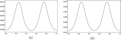
Figure 2. Numerical and exact solutions of Example 1 for N = 40, $\tau =1/1000$ and $T=1/2$ in CGL points.

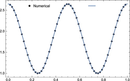
Table 1. Relative errors of $v(x,t)$ for Example 1; $N=40,\tau =1/1000$ and regular grid points

$(x,t)$	$v_{exact}$	$v_{app}$	[16]	Present method
$(1,\frac{1}{1000})$	2.001000	1.990999	1.254372e−05	4.997859e−03
$(\frac{1}{2},\frac{12}{1000})$	2.012072	2.012559	8.098069e−05	2.422318e−04
$(1,\frac{1}{100})$	2.010050	2.007643	1.252541e−04	1.197321e−03
$(\frac{1}{10},\frac{1}{10})$	1.723344	1.722830	3.107279e−04	2.980527e−04
$(1,\frac{1}{10})$	2.105171	2.104739	1.756113e−03	2.051458e−04
$(\frac{1}{3},\frac{1}{9})$	1.279380	1.278830	5.345218e−03	4.291483e−04
$(\frac{2}{3},\frac{1}{9})$	1.279380	1.278832	5.345218e−03	4.280929e−04
$(1,\frac{1}{8})$	2.133148	2.132737	2.635284e−03	1.924323e04
$(\frac{2}{3},\frac{1}{8})$	1.283287	1.282724	5.913283e−03	4.380405e04
$(\frac{7}{8},\frac{1}{6})$	1.590680	1.590156	1.938927e−03	3.291381e−04
$(1,\frac{1}{6})$	2.181360	2.180950	4.463001e−03	1.878411e−04
$(\frac{1}{10},\frac{1}{5})$	1.799418	1.798895	2.587782e−03	2.904718e−04
$(\frac{2}{3},\frac{1}{5})$	1.305351	1.304733	6.505095e−03	4.725092e−04
$(\frac{1}{10},\frac{2}{9})$	1.817382	1.816849	3.694167e−03	2.933668e−04
$(\frac{3}{5},\frac{2}{9})$	1.817382	1.816664	3.634623e−03	3.948590e−04
$(\frac{1}{3},\frac{2}{9})$	1.312212	1.311578	5.713727e−03	4.831508e−04
$(\frac{3}{5},\frac{1}{4})$	1.840405	1.839666	5.269811e−03	4.017101e−04
$(\frac{1}{3},\frac{1}{4})$	1.321006	1.320353	4.886044e−03	4.941974e−04
$(\frac{1}{6},\frac{1}{4})$	1.321006	1.320461	5.775571e−03	4.125653e−04
$(\frac{1}{4},\frac{1}{2})$	1	0.999146	6.996070e−03	8.539304e−04
$(\frac{2}{7},\frac{1}{2})$	1.081637	1.080914	3.425978e−03	6.684268e−04
$(\frac{3}{4},\frac{1}{2})$	1	0.999151	5.194440e−03	8.486204e−04

Table 2. Relative errors of $v(x,t)$, for Example 1; $N=40,\tau =1/1000$ and CGL grid points

t	$r_{exact}$	$r_{app}$	[16]	Present method
$(1,\frac{1}{1000})$	2.001000	2.000996	1.254372e−05	2.244711e−06
$(\frac{1}{2},\frac{12}{1000})$	2.012072	2.012005	8.098069e−05	3.323351e−05
$(1,\frac{1}{100})$	2.010050	2.010009	1.252541e−04	2.002295e−05
$(\frac{1}{10},\frac{1}{10})$	1.723344	1.122964	3.107279e−04	2.200594e−04
$(1,\frac{1}{10})$	2.105171	2.104810	1.756113e−03	1.712410e−04
$(\frac{1}{3},\frac{1}{9})$	1.279380	1.279251	5.345218e−03	1.005594e−04
$(\frac{2}{3},\frac{1}{9})$	1.279380	1.279252	5.345218e−03	9.933721e−05
$(1,\frac{1}{8})$	2.133148	2.132712	2.635284e−03	2.043305e−04
$(\frac{2}{3},\frac{1}{8})$	1.283287	1.283128	5.913283e−03	1.236194e−04
$(\frac{7}{8},\frac{1}{6})$	1.590680	1.590152	1.938927e−03	3.314801e−04
$(1,\frac{1}{6})$	2.181360	2.180820	4.463001e−03	2.474264e−04
$(\frac{1}{10},\frac{1}{5})$	1.799418	1.798794	2.587782e−03	3.466885e−04
$(\frac{2}{3},\frac{1}{5})$	1.305351	1.305052	6.505095e−03	2.280638e−04
$(\frac{1}{10},\frac{2}{9})$	1.817382	1.816716	3.694167e−03	3.664306e−04
$(\frac{3}{5},\frac{2}{9})$	1.817382	1.816473	3.634623e−03	5.001915e−04
$(\frac{1}{3},\frac{2}{9})$	1.312212	1.311880	5.713727e−03	2.524892e−04
$(\frac{3}{5},\frac{1}{4})$	1.840405	1.839442	5.269811e−03	5.231972e−04
$(\frac{1}{3},\frac{1}{4})$	1.321006	1.320637	4.886044e−03	2.793744e−04
$(\frac{1}{6},\frac{1}{4})$	1.321006	1.320408	5.775571e−03	4.523814e−04
$(\frac{1}{4},\frac{1}{2})$	1	0.999522	6.996070e−03	4.779452e−04
$(\frac{2}{7},\frac{1}{2})$	1.081637	1.081202	3.425978e−03	4.016747e−04
$(\frac{3}{4},\frac{1}{2})$	1	0.999520	5.194440e−03	4.795079e−04

Table 3. Relative errors of source parameter $r(t)$ for Example 1; $N=40,\tau =1/1000$ and regular grid points

t	$r_{exact}$	$r_{app}$	[16]	Present method
$\frac{1}{1000}$	1.001000	1.292141	3.027572e−05	1.28954e−05
$\frac{12}{1000}$	1.012000	1.011896	3.202180e−04	1.023366e−04
$\frac{1}{100}$	1.010000	1.010542	2.774495e−04	5.366620e−04
$\frac{1}{10}$	1.100000	1.099358	5.356182e−03	5.835386e−04
$\frac{1}{9}$	1.111111	1.1104521	5.803190e−03	5.923620e−04
$\frac{1}{8}$	1.125000	1.124331	6.494860e−03	5.940311e−04
$\frac{1}{6}$	1.166667	1.165970	8.344175e−03	5.964303e−04
$\frac{1}{5}$	1.200000	1.199274	9.600923e−03	6.042648e−04
$\frac{2}{9}$	1.222222	1.221483	1.040393e−02	6.041307e−04
$\frac{1}{4}$	1.250000	1.249239	1.134528e−02	6.083429e−04

Table 4. Relative errors of source parameter $r(t)$ for Example 1; $N=40,\tau =1/1000$ and CGL grid points

t	$r_{exact}$	$r_{app}$	[16]	Present method
$\frac{1}{1000}$	1.001000	1.001377	3.027572e−05	3.770534e−04
$\frac{12}{1000}$	1.012000	1.012015	3.202180e−04	1.569588e−05
$\frac{1}{100}$	1.010000	1.010042	2.774495e−04	4.236360e−05
$\frac{1}{10}$	1.100000	1.099557	5.356182e−03	4.021124e−04
$\frac{1}{9}$	1.111111	1.111404	5.803190e−03	3.053927e−04
$\frac{1}{8}$	1.125000	1.125189	6.494860e−03	1.683268e−04
$\frac{1}{6}$	1.166667	1.166693	8.344175e−03	7.265121e−05
$\frac{1}{5}$	1.200000	1.199995	9.600923e−03	3.687908e−06
$\frac{2}{9}$	1.222222	1.222211	1.040393e−02	8.834914e−06
$\frac{1}{4}$	1.250000	1.249985	1.134528e−02	1.198785e−05

4.4. Example 2

Consider problem 2 with $\begin{array}{rl}\phi (x)& ={\cos }^2(\pi x),\\ E(t)& =\frac{1}{4}{\mathrm{e}}^t,\\ f(x,t)& =-{\mathrm{e}}^t(2{\pi }^2+{\cos }^2(\pi x)(-4{\pi }^2+t^2)),\\ x^{\ast }& =\frac{1}{3}.\end{array}$ The exact solution is given by $\left\{v(x,t),p(t)\right\}=\left\{{\mathrm{e}}^t{\cos }^2(\pi x),1+t^2\right\}.$ This example is also approximated similar to Example 1 with two sets of grid points, namely, CGL grid points and regular grid points. In Tables 5 and 6, the approximation of the proposed method for $v(x,t)$ is compared to that in [16]. In Tables 7 and 8, the approximation of the method for $p(t)$ is compared to that in [16]. In Figure 3, numerical and exact solutions are drawn at time $T=1/2$. To demonstrate the sensitivity of the method to errors, we give a perturbation ${10}^{-2}$ to the right-side function $f(x,t)$ and over-specified condition $E(t)$. Figure 4(b) shows that the method is stable.

Figure 3. Absolute error graphs of v in Example 2 at time $T=1/2$ for N = 15 and $\tau =1/5000$ in CGL points: (a) without noisy data and (b) with noisy data.

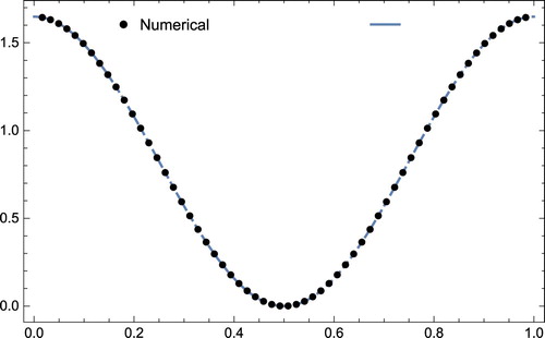
Figure 4. Numerical and exact solutions of Example 2 for $N=15,$ $\tau =1/5000$ and $T=1/2$ in CGL points.

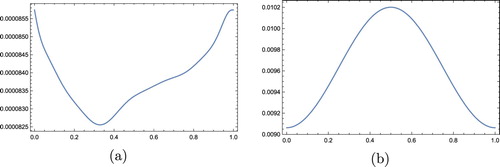
Table 5. Relative errors of $v(x,t)$ for Example 2; $N=15,\tau =1/5000$ and regular grid points

$(x,t)$	$v_{exact}$	$v_{app}$	[16]	Present method
$(1,\frac{1}{1000})$	1.001000	1.000998	3.634763e−05	2.124565e−06
$(\frac{1}{2},\frac{12}{1000})$	0	0.000335	–	–
$(1,\frac{1}{100})$	1.010050	1.009966	3.669768e−04	8.238902e−05
$(\frac{1}{10},\frac{1}{10})$	0.999636	0.999262	3.743112e−04	3.743112e−04
$(1,\frac{1}{10})$	1.105171	1.105114	3.176440e−03	5.133585e−05
$(\frac{1}{3},\frac{1}{9})$	0.279380	0.279323	6.915318e−07	2.001190e−04
$(\frac{2}{3},\frac{1}{9})$	0.279380	0.279323	1.003347e−04	2.005758e−04
$(1,\frac{1}{8})$	1.133148	1.133090	3.155529e−03	5.130210e−05
$(\frac{2}{3},\frac{1}{8})$	0.283287	0.283230	1.438367e−04	2.010074e−04
$(\frac{7}{8},\frac{1}{6})$	1.008354	1.008158	2.290763e−03	1.945543e−04
$(1,\frac{1}{6})$	1.181360	1.181299	2.431706e−03	5.137710e−05
$(\frac{1}{10},\frac{1}{5})$	1.104769	1.104355	1.025735e−03	3.741129e−04
$(\frac{2}{3},\frac{1}{5})$	0.305351	0.305289	1.951084e−04	2.017787e−04
$(\frac{1}{10},\frac{2}{9})$	0.112959	1.129171	1.039568e−04	3.741372e−04
$(\frac{3}{5},\frac{2}{9})$	0.119254	0.119191	5.718319e−04	5.274899e−04
$(\frac{1}{3},\frac{2}{9})$	0.312212	0.312149	1.178045e−06	2.001556e−04
$(\frac{3}{5},\frac{1}{4})$	0.122613	0.122548	4.727312e−03	5.277928e−04
$(\frac{1}{3},\frac{1}{4})$	0.321006	0.320942	2.740444e−06	2.001663e−04
$(\frac{1}{6},\frac{1}{4})$	0.963019	0.962725	1.825324e−03	3.043692e−04
$(\frac{1}{4},\frac{1}{2})$	0.824361	0.824242	3.738026e−02	1.438332e−04
$(\frac{2}{7},\frac{1}{2})$	0.640923	0.640977	2.668476e−02	8.442645e−05
$(\frac{3}{4},\frac{1}{2})$	0.824361	0.824240	3.693455e−02	1.452184e−04

Table 6. Relative errors of $v(x,t)$ for Example 2; $N=15,\tau =1/5000$ and CGL grid points

$(x,t)$	$v_{exact}$	$v_{app}$	[16]	Present method
$(1,\frac{1}{1000})$	1.001000	1.000985	3.634763e−05	1.537601e−05
$(\frac{1}{2},\frac{12}{1000})$	0	0.002044	–	–
$(1,\frac{1}{100})$	1.010050	1.009953	3.669768e−04	9.566978e−05
$(\frac{1}{10},\frac{1}{10})$	0.999636	0.999520	3.743112e−04	1.164640e−04
$(1,\frac{1}{10})$	1.105171	1.105114	3.176440e−03	5.068616e−05
$(\frac{1}{3},\frac{1}{9})$	0.279380	0.279569	6.915318e−07	6.803728e−04
$(\frac{2}{3},\frac{1}{9})$	0.279380	0.279569	1.003347e−04	6.799966e−04
$(1,\frac{1}{8})$	1.133148	1.133091	3.155529e−03	5.060933e−05
$(\frac{2}{3},\frac{1}{8})$	0.283287	0.283479	1.438367e−04	6.796107e−04
$(\frac{7}{8},\frac{1}{6})$	1.008354	1.007991	2.290763e−03	3.594921e−04
$(1,\frac{1}{6})$	1.181360	1.181300	2.431706e−03	5.061205e−05
$(\frac{1}{10},\frac{1}{5})$	1.104769	1.104640	1.025735e−03	1.161943e−04
$(\frac{2}{3},\frac{1}{5})$	0.305351	0.305557	1.951084e−04	6.788711e−04
$(\frac{1}{10},\frac{2}{9})$	0.112959	1.129463	1.039568e−04	1.162056e−04
$(\frac{3}{5},\frac{2}{9})$	0.119254	0.121068	5.718319e−04	1.521541e−02
$(\frac{1}{3},\frac{2}{9})$	0.312212	0.312424	1.178045e−06	6.803400e−04
$(\frac{3}{5},\frac{1}{4})$	0.122613	0.124479	4.727312e−03	1.521627e−02
$(\frac{1}{3},\frac{1}{4})$	0.321006	0.321224	2.740444e−06	6.803309e−04
$(\frac{1}{6},\frac{1}{4})$	0.963019	0.962939	1.825324e−03	8.243972e−05
$(\frac{1}{4},\frac{1}{2})$	0.824361	0.824277	3.738026e−02	1.003791e−04
$(\frac{2}{7},\frac{1}{2})$	0.640923	0.641493	2.668476e−02	8.899443e−04
$(\frac{3}{4},\frac{1}{2})$	0.824361	0.824276	3.693455e−02	1.015589e−04

Table 7. Relative errors of source parameter $p(t)$ for Example 2; $N=15,\tau =1/5000$ and regular grid points

t	$p_{exact}$	$p_{app}$	[16]	Present method
$\frac{1}{1000}$	1.000001	0.974267	1.761649e−04	2.573396e−02
$\frac{12}{1000}$	1.000144	1.000137	1.878036e−04	6.573181e−06
$\frac{1}{100}$	1.000100	0.999376	1.844624e−04	7.235768e−04
$\frac{1}{10}$	1.010000	1.010127	1.126239e−03	1.260774e−04
$\frac{1}{9}$	1.012346	1.012479	2.427768e−03	1.320850e−04
$\frac{1}{8}$	1.015625	1.015765	6.019765e−03	1.380792e−04
$\frac{1}{6}$	1.027778	1.027932	2.323355e−02	1.503308e−04
$\frac{1}{5}$	1.040000	1.040165	3.425239e−03	1.592648e−04
$\frac{2}{9}$	1.049383	1.049556	4.395779e−02	1.652488e−04
$\frac{1}{4}$	1.062500	1.062682	6.325459e−03	1.718720e−04

Table 8. Relative errors of source parameter $p(t)$ for Example 2; $N=15,\tau =1/5000$ and CGL grid points

t	$p_{exact}$	$p_{app}$	[16]	Present method
$\frac{1}{1000}$	1.000001	0.973126	1.761649e−04	2.687455e−02
$\frac{12}{1000}$	1.000144	1.000555	1.878036e−04	4.112742e−04
$\frac{1}{100}$	1.000100	0.999809	1.844624e−04	2.902477e−04
$\frac{1}{10}$	1.010000	1.010103	1.126239e−03	1.023528e−04
$\frac{1}{9}$	1.012346	1.012464	2.427768e−03	1.176213e−04
$\frac{1}{8}$	1.015625	1.015738	6.019765e−03	1.122422e−04
$\frac{1}{6}$	1.027778	1.027909	2.323355e−02	1.277133e−04
$\frac{1}{5}$	1.040000	1.040141	3.425239e−03	1.361278e−04
$\frac{2}{9}$	1.049383	1.049530	4.395779e−02	1.405234e−04
$\frac{1}{4}$	1.062500	1.062609	6.325459e−03	1.030532e−04

5. Conclusion

In this paper, the proposed method was applied successfully to solve two coefficient parabolic inverse problems with a nonlocal boundary condition. The results of the examples are better than those of the previous paper. The present method is shown to be easy to program, great convergence, easy to treat the boundary conditions, and stable w.r.t noise. This method can be applied to higher dimensional inverse problems that are left to our further works.

Acknowledgments

We are grateful to the anonymous reviewers for their helpful comments, which undoubtedly led to the definite improvement in the manuscript.

Disclosure statement

No potential conflict of interest was reported by the authors.

References

- Bal G, Schotland JC. Inverse scattering and acousto-optic imaging. Phys Rev Lett. 2010; 104:043902. doi: 10.1103/PhysRevLett.104.043902
- Baraniuk R, Steeghs P. Compressive radar imaging. In: Radar conference. Boston (MA): IEEE; 2007. p. 128–133.
- Isakov V, Wu SF. On theory and application of the Helmholtz equation least squares method in inverse acoustics. Inverse Probl. 2002;18(4):1147–1159. doi: 10.1088/0266-5611/18/4/313
- Widrow B, Walach E. Adaptive inverse control, reissue edition: a signal processing approach. Hoboken (NJ): John Wiley & Sons, Inc.; 2008.
- Crossen E, Gockenbach MS, Jadamba B, et al. An equation error approach for the elasticity imaging inverse problem for predicting tumor location. Comput Math Appl. 2014; 67(1):122–135. doi: 10.1016/j.camwa.2013.10.006
- Berntsson F, Baravdish G. Coefficient identification in PDEs applied to image inpainting. Appl Math Comput. 2014;242:227–235.
- García E, Amaya I, Correa R. Estimation of thermal properties of a solid sample during a microwave heating process. Appl Therm Eng. 2018;129:587–595. doi: 10.1016/j.applthermaleng.2017.10.037
- Yousefi SA. Finding a control parameter in a one-dimensional parabolic inverse problem by using the Bernstein Galerkin method. Inverse Probl Sci Eng. 2009;17(6):821–828. doi: 10.1080/17415970802583911
- Dehghan M. Parameter determination in a partial differential equation from the overspecified data. Math Comput Model. 2005;41(2–3):196–213. doi: 10.1016/j.mcm.2004.07.010
- Lerma A A, Hinestroza D. Coefficient identification in the Euler-Bernoulli equation using regularization methods. Appl Math Model. 2017;41:223–235. doi: 10.1016/j.apm.2016.08.035
- Dehghan M, Tatari M. Determination of a control parameter in a one-dimensional parabolic equation using the method of radial basis functions. Math Comput Model. 2006;44(11–12):1160–1168. doi: 10.1016/j.mcm.2006.04.003
- Mohammadi M, Mokhtari R, Toutian Isfahani F. Solving an inverse problem for a parabolic equation with a nonlocal boundary condition in the reproducing kernel space. IJNAO. 2014;4:57–76.
- Wang S, Lin Y. A finite-difference solution to an inverse problem for determining a control function in a parabolic partial differential equation. Inverse Probl. 1989;5(4):631–640. doi: 10.1088/0266-5611/5/4/013
- Cannon JR, Lin Y, Wang S. Determination of source parameter in parabolic equations. Meccanica. 1992;27(2):85–94. doi: 10.1007/BF00420586
- Kanca F, Ismailov MI. The inverse problem of finding the time-dependent diffusion coefficient of the heat equation from integral overdetermination data. Inverse Probl Sci Eng. 2012;20(4):463–476. doi: 10.1080/17415977.2011.629093
- Mohammadi M, Mokhtari R, Panahipour H. Solving two parabolic inverse problems with a nonlocal boundary condition in the reproducing kernel space. Appl Comput Math. 2014;13(1):91–106.
- Cui MG, Lin YZ, Yang LH. A new method of solving the coefficient inverse problem. Sci China Ser A: Math. 2007;50(4):561–572. doi: 10.1007/s11425-007-0013-8
- Abbasbandy S. A new class of polynomial functions equipped with a parameter. Math Sci. 2017;11:127–130. doi: 10.1007/s40096-017-0217-1
- Yuzbasi S, Sahin N. On the solutions of a class of nonlinear ordinary differential equations by the Bessel polynomials. J Numer Math. 2012;20:55–80. doi: 10.1515/jnum-2012-0003
- Hajishafieiha J, Abbasbandy S. A new class of polynomial functions for approximate solution of generalized Benjamin-Bona-Mahony-Burgers (gBBMB) equations. Appl Math Comput. doi:10.1016/J.AMC.2019.124765
- Strikwerda JC. Finite difference schemes and partial differential equations. Philadelphia: Siam; 2004.