Real-time inverse solution of the composites’ cure heat transfer problem under uncertainty

Abstract

This paper addresses the development of an inversion scheme based on Markov Chain Monte Carlo integrating process modelling with monitoring data for the real-time probabilistic estimation of unknown stochastic input parameters such as heat transfer coefficient and resin thermal conductivity and process outcomes during the manufacture of fibrous composites materials. Kriging was utilized to build an efficient surrogate model of the composite curing process based on finite element modelling. The utilization of an inverse scheme with real-time temperature monitoring driving the estimation of process parameters during manufacture results in real-time probabilistic prediction of process outcomes.

KEYWORDS:

• Composites manufacturing
• curing
• uncertainty estimation
• inverse analysis
• Markov chain Monte Carlo

AMS/MSC SUBJECT CLASSIFICATION CODES:

• 62F15
• 62L20
• 97N50

1. Introduction

The manufacturing of fiber-reinforced thermosetting matrix composites involves several stages such as lay-up, draping, resin impregnation or consolidation and curing. The cure process is a non-linear heat transfer effect in which the thermosetting polymer resin reacts exothermically and is transformed from an oligomeric liquid to a glassy solid. The quality of the final part depends strongly on phenomena taking place during the cure governed by manufacturing process parameters and boundary conditions. The selection of cure process parameters is crucial for eliminating potential induced defects such as undercure or thermal overshoot in thick components.

Inherent process and raw material uncertainty affect process time and product quality [1]. Boundary conditions can present significant variability which can induce considerable variations in the process outcome [2,3]. Variations of environmental conditions during composites manufacturing can introduce variations in the surface heat transfer coefficient with a coefficient of variation of about 18% [2] which in turn can cause significant variability in cure duration reaching a coefficient of variation of 20% [3]. Also, the conductivity of the curing composite is difficult to measure or predict and is subject to significant variations as a result of variability in the architecture of the consolidated reinforcement. Uncertainty in cure kinetics parameters, such as initial degree of cure, can introduce significant variations in exothermic effects in cases of thick components reaching coefficients of variation of approximately 30% [4].

Cure monitoring techniques have been developed to measure critical properties during the curing stage such as the crosslinking reaction progress [5] within the composite component during the process. The integration of process monitoring with modelling into an inverse scheme has been used for material characterization linked to preform permeability [6–8] and thermal properties [9].

Inversion schemes based on Bayesian inference have been developed to address potentially ill-posed inverse heat transfer problems for the estimation of material properties and boundary conditions [10–13]. Bayesian inference operates as a sampler and addresses ill-posedness by incorporating prior knowledge about the parameters’ values. Inverse schemes require a significant number of iterations making the use of the whole model computationally cumbersome. Surrogate models such as response surfaces, Kriging and non-uniform rational B-splines (NURBs) address this problem.

In the present paper, an inverse heat transfer scheme is developed incorporating process monitoring signals and process modelling for the real-time estimation of resin thermal conductivity levels, surface heat transfer coefficient and cure process duration variability during the cure of a flat composite part. A surrogate model is used, based on Kriging, substituting the FE model and minimizing the computational time of the inverse solution. The inversion procedure was implemented and tested in the case of the resin transfer moulding (RTM) of a glass fibre-reinforced epoxy composite.

2. Methodology

2.1. Processing

The RTM process was utilized for manufacturing experiments. In this process, resin impregnates a dry preform placed in a sealed rigid mould under pressure, subsequently curing occurs with further heating of the mould upon completion of filling. A rectangular mould cavity with dimensions 900 × 340 × 3.3 mm was used. The sides of the cavity were sealed using silicone rubber, whilst the tool was closed using a glass top plate and a set of stiffeners ensured uniform thickness of the composite plate. In this set-up heating is achieved by an array of heating elements placed under the mould cavity. The specific experimental configuration was selected in order to reduce the heat transfer problem to one-dimension. The preform comprised two layers of E-TX1769 (BTI Europe) tri-axial E-glass fabric [14] with a surface density of 1770 g/m² and total lay-up sequence [ + 45°/−45°/0°/0°/−45°/+45°] resulting in a fibre weight fraction of 62% at a thickness of 3.3 mm. The matrix was Hexcel HexFlow^® RTM6 epoxy resin [15]. Resin filling was carried out at 120°C. After filling completion, the material was cured at 160°C. The heating ramp rate from 120°C to 160°C was 1.5°C/min and the duration of the dwell was 90 min. Three K-type thermocouples were placed at the lower surface of the curing material, at mid-thickness and on the top layer in contact with the upper tool to monitor the temperature evolution up to the completion of cure.

2.2. Cure simulation

The dominant heat transfer mechanism in the cure process of composite materials is conduction since buoyancy convection plays a negligible role. The governing energy balance is (1) $\rho c_p\frac{\mathrm{\partial }T}{\mathrm{\partial }t}=\overline{\mathrm{\nabla }}\left(\mathbf{\text{K}}\mathrm{\nabla }T\right)+\left(1-v_{\mathrm{f}}\right){\rho }_{\mathrm{r}}{H}_{\text{tot}}\frac{\text{d}\alpha }{\text{d}t}$(1) where $\rho$ is the density of the composite, $c_p$ is the specific heat capacity, $T$ the temperature, $\mathbf{\text{K}}$ the thermal conductivity tensor, $v_{\mathrm{f}}$ the fibre volume fraction, ${\rho }_{\mathrm{r}}$ the resin density, $H_{\text{tot}}$ the total heat of the curing reaction and $\alpha$ the degree of cure. The second term in the right-hand side of Equation (1) expresses the heat generated due to the exothermic crosslinking reaction, where $\text{d}\alpha /\text{d}t$ represents the curing reaction rate.

Three types of boundary conditions can be applied to the general case: (i) prescribed temperature, (ii) convection and (iii) prescribed heat flux. The prescribed temperature boundary condition is expressed as follows: (2) $T\left(\mathbf{\text{d}},t\right)=T_{\mathrm{b}}\left(\mathbf{\text{d}},t\right),\mathbf{\text{d}}\in D_1$(2) where $\mathbf{\text{d}}$ denotes the spatial coordinates at the boundary D₁, whilst $T_{\mathrm{b}}$ is the prescribed temperature. The convection boundary condition is (3) $-{\mathbf{\text{n}}}_{\mathbf{\text{sv}}}\mathbf{\text{K}}\mathrm{\nabla }T\left(\mathbf{\text{d}},t\right)=h\left(T\left(\mathbf{\text{d}},t\right)-T_{\mathrm{\infty }}\right),\mathbf{\text{d}}\in D_2$(3) where ${\mathbf{\text{n}}}_{\mathbf{\text{sv}}}$ denotes the surface vector at the boundary $D_2$, $\text{h}$ the surface heat transfer coefficient and $T_{\mathrm{\infty }}$ the ambient temperature. The prescribed heat flux ($q$) condition is expressed as follows: (4) $-{\mathbf{\text{n}}}_{\mathbf{\text{sv}}}\mathbf{\text{K}}\mathrm{\nabla }T\left(\mathbf{\text{d}},t\right)=q\left(\mathbf{\text{d}},t\right),\mathbf{\text{d}}\in D_3$(4) where (5) $D_1\cup D_2\cup D_3=D$(5) where D is the boundary of the whole domain, and $D_1$, $D_2$, $D_3$ the corresponding parts of the boundary at which the prescribed temperature, convection and prescribed heat flux conditions apply, respectively.

A thermal cure simulation model was implemented in the finite element solver MSC.Marc to simulate the cure. Figure 1 illustrates a schematic representation of the model geometry. The model comprises two parts; a composite flat laminate and the glass top plate of the mould. The composite part is represented by 6 3D iso-parametric eight-noded composite brick elements (175 MSC.Marc element type [16]). Each element represents one ply of E-glass with 0.55 mm nominal thickness. Boundary conditions corresponding to the time-dependent prescribed temperature applied to the lower boundary of the curing material and natural air convection applied to the top of the glass tooling plate are implemented using user subroutines FORCDT and UFILM, respectively [17]. The heat transfer coefficient is an effective parameter combining natural convection and radiation. Due to the isothermal character of the manufacturing process convection coefficient dependence on temperature was neglected. The predefined thermal profile comprises an initial dwell at 120°C for 30 min to ensure equilibration of the temperature gradient in the thickness direction. A heating ramp of 1.5°C/min was applied from 120°C to 160°C followed by a 90 min dwell. The initial degree of cure in the model was 2%. The heat transfer problem is one dimensional due to symmetry. The thermal properties of the glass top plate are reported in Table 1 [9].

Figure 1. Schematic representation of the model.

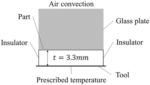
Table 1. Glass top plate thermal properties and boundary condition parameters [9].

Properties	Value	Units
Density	2.7	g cm^−3
Specific heat capacity	0.84	J  g^−1°C^−1
Thermal conductivity	0.78	W  m^−  ^1°C^−1
Heat transfer coefficient	8.5	W  m^−2  °C^−1

User subroutines UCURE, USPCHT and ANKOND were used for the integration of material sub-models, cure reaction kinetics, specific heat capacity and thermal conductivity, respectively [17]. The cure kinetics model is a combination of an nth order model and an autocatalytic model [18]. The cure reaction rate in the cure kinetic models is calculated as follows: (6) $\frac{\text{d}\alpha }{\text{d}t}=k_1(1-\alpha {)}^{{\text{n}}_1}+k_2(1-\alpha {)}^{{\text{n}}_2}{\alpha }^{\text{m}}$(6) where $m,n_1,n_2$ are the reaction orders, $k_1$ and $k_2$ the reaction rate constants expressed as (7) $\frac{1}{k_{1,2}}=\frac{1}{A_{1,2}{e}^{\left(-E_{1,2}/RT\right)}}+\frac{1}{A_d{e}^{\left(-E_d/RT\right)}{e}^{\left(-b/f\right)}}$(7) Here $A_{\mathbf{1}\mathbf{,}\mathbf{2}}$ and $A_{\mathrm{d}}$ denote pre-exponential factors, $E_{\mathbf{1}\mathbf{,}\mathbf{2}}$ and $E_{\mathrm{d}}$ the activation energies for chemical reactions and diffusion, respectively, $b$ is a fitting parameter, $R$ the universal gas constant and $f$ the equilibrium free volume computed as follows: (8) $f=w\left(T-T_g\right)+g$(8) where $w$ and $g$ are constants and $T_g$ is the instantaneous glass transition temperature expressed as [19] (9) $T_g=T_{g0}+\frac{\left(T_{g\mathrm{\infty }}-T_{g0}\right)\lambda \alpha }{1-\left(1-\lambda \right)\alpha }$(9) where $T_{g\mathrm{\infty }}$ and $T_{\text{g}0}$ are the glass transition temperature of the fully cured and uncured material and $\lambda$ is a parameter controlling the convexity of the dependence.

The specific heat capacity of the composite is calculated using the rule of mixtures as follows: (10) $c_p=w_f{c}_{pf}+\left(1-w_f\right)c_{pr}$(10) where $c_{pf}$ is the fibre specific heat capacity, $c_{pr}$ the specific heat capacity of the resin and ${\mathbf{\text{w}}}_{\mathrm{f}}$ the weight fraction. The specific heat capacities of the resin and the fibre are computed using: (11) $\begin{array}{rl}{c}_{pf}& =A_{f{c}_p}T+B_{f{c}_p}\end{array}$(11) (12) $\begin{array}{rl}{c}_{pr}& =A_{r{c}_p}T+B_{rcp}+\frac{{\mathrm{\Delta }}_{r{c}_p}}{1+e^{C_{r{c}_p}\left(T-T_g-{\text{σ}}_r\right)}}\end{array}$(12) where $A_{f{c}_p}$, $B_{f{c}_p}$ define the linear dependence of fibre specific heat capacity on temperature, $A_{r{c}_p}$, $B_{r{c}_p}$ control the linear dependence of the specific heat capacity of the uncured resin on temperature and $A_{r{c}_p}$, $C_{r{c}_p}$ and ${\text{σ}}_r$ are the strength, width and temperature shift of the specific heat capacity step occurring at resin vitrification [4]. The composite density can be computed using the density of the resin ${\rho }_r$ and carbon fibre ${\rho }_f$ [14,15]: (13) $\rho =\frac{{\rho }_r{\rho }_f}{v_f{\rho }_r+\left(1-v_f\right){\rho }_f}$(13) The thermal conductivity of the anisotropic composite material in the transverse direction is calculated as follows [20]: (14) $K=v_f{K}_r\left(\frac{K_{tf}}{K_r}-1\right)+K_r\left(\frac{1}{2}-\frac{K_{tf}}{2K_r}\right)+K_r\left(\frac{K_{tf}}{K_r}1\right)\sqrt{{v_f}^2-v_f+\frac{{\left(\frac{K_{tf}}{K_r}+1\right)}^2}{{\left(\frac{2K_{tf}}{K_r}-2\right)}^2}}$(14) where $K_{tf}$ is the thermal conductivity of the fibre in the radial direction and $K_r$ the resin thermal conductivity. The dependence of thermal conductivity of the resin on temperature and degree of cure can be expressed as [9] (15) $K_r=k_{e}T{\alpha }^2-k_{d}T\alpha -k_{c}T-k_b{\alpha }^2+k_a\alpha +k$(15) The intercept $k$ in Equation (15) controls the overall level of conductivity and governs its variability. In the experimental scatter presented in the early stages of resin conductivity characterization, the degree of cure is low, leading to significant uncertainty of the resin thermal conductivity intercept estimation. Furthermore, the parameter k variability is driven by the present of local imperfections on fibre architecture due to handling and storage, nesting effects during lay-up and preform misplacement. The parameter $k_c$ depends only on the composite temperature which presents less variability and thus has not been considered as a stochastic parameter. In addition, the surface heat transfer coefficient presents significant variability affecting cure process outcomes. This variability is attributed to varying environmental conditions during the manufacturing process [2] resulting in considerable deviation around theoretical values. Therefore, the thermal conductivity intercept and the surface heat transfer coefficient were considered as unknown stochastic parameters in the inversion scheme. Material constants involved in Equations (2)–(15) are reported in Table 2 [4,9,14,15,21].

Table 2. Parameter values for the cure kinetics [4], glass transition temperature, specific heat capacity [21], thermal conductivity [9] and density [14,15] material models.

Parameter	Value
Total heat reaction: ${\text{{H}}}_{\text{{{tot}}}}$ [18]	$400\left(\text{J}{\text{g}}^{-1}\right)$
Pre-exponential factor of the nth order term [4]: ${\text{{A}}}_1$	$\mathrm{19,000}\left({\text{s}}^{-1}\right)$
Pre-exponential factor of the autocatalytic term [4]: ${\text{{A}}}_2$	$\mathrm{22,080}\left({\text{s}}^{-1}\right)$
Pre-exponential factor of diffusion [4]: ${\text{{A}}}_{\text{{d}}}$	$6.76{10}^{18}\left({\text{s}}^{-1}\right)$
Activation energy of the nth order term [4]: ${\text{{E}}}_1$	$\mathrm{72,900}\left(\text{Jmo}{\text{l}}^{-1}\right)$
Activation energy of the autocatalytic term [4]: ${\text{{E}}}_2$	$\mathrm{57,820}\left(\text{Jmo}{\text{l}}^{-1}\right)$
Activation energy of diffusion [4]: ${\text{{E}}}_{\text{{d}}}$	$13,8{10}^3\left(\text{Jmo}{\text{l}}^{-1}\right)$
Autocatalytic reaction order [4]: $\text{{m}}$	$1.29$
Reaction order of the nth order term [4]: ${\text{{n}}}_1$	$1.97$
Reaction order of the autocatalytic term [4]: ${\text{{n}}}_2$	$1.53$
Exponent of diffusion term [4]: $\text{{b}}$	$0.452$
Equilibrium free volume model slope [4]: w	$48{10}^{-5}\left(1{\text{K}}^{-1}\right)$
Equilibrium free volume model intercept [4]: g	$0.025$
Glass transition temperature of uncured material [4]: ${\text{{T}}}_{\text{{g}}0}$	$-11\left({}^{\circ }\text{C}\right)$
Glass transition temperature of fully cured material [4]: ${\text{{T}}}_{\text{{g}}\mathrm{\infty }}$	$206\left({}^{\circ }\text{C}\right)$
Glass transition temperature convexity constant [4]: $\mathit{\lambda }$	$0.435$
Fiber specific heat capacity model slope [21]: ${\text{{A}}}_{\text{{f}}{\text{{c}}}_{\text{{p}}}}$	$14{10}^{-4}\left(\text{J}{{\text{g}}^{-1}}^{\circ }{\text{C}}^{-2}\right)$
Fiber specific heat capacity model intercept [21]: ${\text{{B}}}_{\text{{f}}{\text{{c}}}_{\text{{p}}}}$	$0.841\left(\text{J}{{\text{g}}^{-1}}^{\circ }{\text{C}}^{-2}\right)$
Resin specific heat capacity model slope [21]: ${\text{{A}}}_{\text{{r}}{\text{{c}}}_{\text{{p}}}}$	$25{10}^{-4}\left(\text{J}{{\text{g}}^{-1}}^{\circ }{\text{C}}^{-2}\right)$
Resin specific heat capacity model intercept [21]: ${\text{{B}}}_{\text{{r}}{\text{{c}}}_{\text{{p}}}}$	$1.8\left(\text{J}{{\text{g}}^{-1}}^{\circ }{\text{C}}^{-2}\right)$
Resin specific heat capacity model step [21]: ${\mathit{\Delta }}_{\text{{r}}{\text{{c}}}_{\text{{p}}}}$	$-0.25\left(\text{J}{{\text{g}}^{-1}}^{\circ }{\text{C}}^{-2}\right)$
Resin specific heat capacity model step breadth [21] parameter: ${\text{{C}}}_{\text{{r}}{\text{{c}}}_{\text{{p}}}}$	$1.1\left({}^{\circ }{\text{C}}^{-1}\right)$
Resin specific heat capacity model step shift parameter [21]: ${\text{σ}}_{\text{{r}}}$	$16.5\left({}^{\circ }\text{C}\right)$
Resin thermal conductivity model quadratic coupling [9]: ${\text{{k}}}_{\text{{e}}}$	$0.0008\left(\text{W}{{\text{m}}^{-1}}^{\circ }{\text{C}}^{-2}\right)$
Resin thermal conductivity model coupling constant [9]: ${\text{{k}}}_{\text{{d}}}$	$-0.0011\left(\text{W}{{\text{m}}^{-1}}^{\circ }{\text{C}}^{-2}\right)$
Resin thermal conductivity model linear temperature constant [9]: ${\text{{k}}}_{\text{{c}}}$	$-0.0002\left(\text{W}{{\text{m}}^{-1}}^{\circ }{\text{C}}^{-2}\right)$
Resin thermal conductivity model quadratic conversion constant [9]: ${\text{{k}}}_{\text{{b}}}$	$-0.0937\left(\text{W}{{\text{m}}^{-1}}^{\circ }{\text{C}}^{-1}\right)$
Resin thermal conductivity model linear conversion constant [9]: ${\text{{k}}}_{\text{{a}}}$	$0.22\left(\text{W}{{\text{m}}^{-1}}^{\circ }{\text{C}}^{-1}\right)$
Resin thermal conductivity model intercept [9]: $\text{{k}}$	$0.12\left(\text{W}{{\text{m}}^{-1}}^{\circ }{\text{C}}^{-1}\right)$
Resin density [14]: ${\mathit{\rho }}_{\text{{r}}}$	$1.11\left(\text{gm}{\text{l}}^{-1}\right)$
Fibre density [15]: ${\mathit{\rho }}_{\text{{f}}}$	$2.54\left(\text{gm}{\text{l}}^{-1}\right)$

2.3. Surrogate model

Cure process simulation using non-linear FE analysis is computationally expensive. Inversion procedures such as Markov Chain Monte Carlo (MCMC) require a large number of cure model evaluations and use of the FE model becomes a limiting factor. Surrogate models were developed in this work based on Kriging to address this issue by substituting the FE model. Kriging enables a prediction of untried sample values to be made without bias, with minimum variance and more accurately than low-order polynomial regression models. Figure 2 summarizes the procedure implemented in this work. The construction of the surrogate model requires a set of design points and their response as inputs. Latin hypercube sampling (LHS) was selected for generating a sample of $N$ input points, whilst the FE model was used to compute the response at these points. Three surrogate models were constructed. The input variables of the first and second surrogate models include the unknown stochastic parameters k and h and the cure time $\left(t\right)$, whilst the outputs are the temperature at mid-thickness ($T_{\text{mid}})$ and on the top surface ($T_{\text{top}})$ of the curing composite component. The third surrogate model computes the minimum final degree of cure $\left({\alpha }_{\text{fmin}}\right)$ as a function of the unknown stochastic variables k and h. The minimum final degree of cure is defined as the minimum degree of cure over the volume of the part at the end of the process. Its practical significance is related to the final glass transition temperature reached at the end of the process, which governs the softening temperature of the composite material beyond which the component cannot play a structural role. Table 3 summarizes the parameters of the surrogate models and their ranges. Considering the relatively small dimensionality of the problem a sample of 2000 points was selected.

Figure 2. Surrogate model construction methodology.

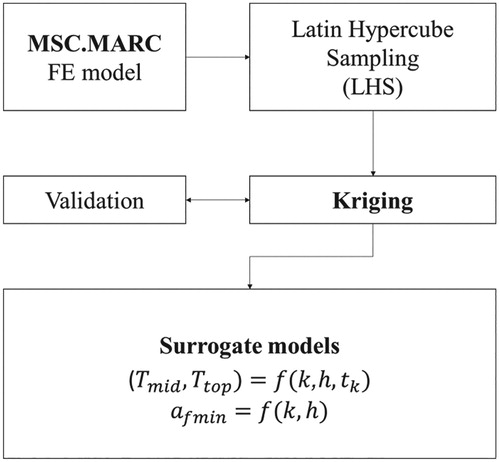
Table 3. Surrogate models’ parameters and their ranges.

Parameter		Range
Thermal conductivity level	$k$ (Wm^−1°C^−1)	0.01–0.2
Heat transfer coefficient	h (Wm^−2°C^−1)	3–21
Cure time	t (min)	0–110

Table 4. MCMC parameter values.

Parameter		Value
Likelihood distribution standard deviation	${\text{σ}}_{\text{exp}}$	1 (°C)
Thermal conductivity prior mean value	${\mu }_{\text{prior}}^{\text{k}}$	0.12 ($\text{W}{{\text{m}}^{-1}}^{\circ }{\text{C}}^{-1}$)
Heat transfer coefficient prior mean value	${\mu }_{\text{prior}}^{\text{h}}$	8.5 ($\text{W}{{\text{m}}^{-2}}^{\circ }{\text{C}}^{-1}$)
Thermal conductivity level prior standard deviation	${\text{σ}}_{\text{prior}}^{\text{k}}$	0.02 ($\text{W}{{\text{m}}^{-1}}^{\circ }{\text{C}}^{-1}$)
Heat transfer coefficient prior mean value	${\text{σ}}_{\text{prior}}^{\text{h}}$	1.5 ($\text{W}{{\text{m}}^{-2}}^{\circ }{\text{C}}^{-1}$)
Initial noise level ${\text{ε}}_{\mathrm{k}}$ standard deviation	${{\text{σ}}_{\text{ε}}}_{\mathrm{k}}$	0.02 ($\text{W}{{\text{m}}^{-1}}^{\circ }{\text{C}}^{-1}$)
Initial noise level ${\text{ε}}_{\mathrm{h}}$ standard deviation	${{\text{σ}}_{\text{ε}}}_{\mathrm{h}}$	1.5 ($\text{W}{{\text{m}}^{-2}}^{\circ }{\text{C}}^{-1}$)
Initial thermal conductivity level	$k_0$	0.12 ($\text{W}{{\text{m}}^{-1}}^{\circ }{\text{C}}^{-1}$)
Initial heat transfer coefficient	$h_0$	8.5 ($\text{W}{{\text{m}}^{-2}}^{\circ }{\text{C}}^{-1}$)
Total number of experimental data of each thermocouple	$N_{\mathrm{k}}$	110
Parallel chains	$n_{\text{ch}}$	4
Total number of MCMC iterations	$M$	210,000
MCMC iterations for swap algorithm initiation	$n_{\mathrm{s}}$	1000

Kriging expresses the surrogate model responses $Y_1\left({\mathbf{\text{x}}}_1\right)$ and $Y_2\left({\mathbf{\text{x}}}_2\right)\in {\mathbb{R}}^2$, ($T_{\text{mid}}$ and $T{}_{\text{top}})$ and $Y_3\left({\mathbf{\text{x}}}_3\right)\in \mathbb{R}$ (${\alpha }_{\text{fmin}})$ with the input vectors ${\mathbf{\text{x}}}_1,{\mathbf{\text{x}}}_2=\left[k,h,t\right],{\mathbf{\text{x}}}_1,{\mathbf{\text{x}}}_2\in {\mathbb{R}}^3$ and ${\mathbf{\text{x}}}_3=\left[k,h\right],{\mathbf{\text{x}}}_3\in {\mathbb{R}}^2$ as follows: (16) ${\mathbf{\text{Y}}}_{\mathbf{\text{i}}}\left({\mathbf{\text{x}}}_{\mathbf{\text{i}}}\right)={\mathbf{\text{f}}}_{\mathbf{\text{i}}}({\mathbf{\text{x}}}_{\mathbf{\text{i}}}{)}^{\mathbf{\text{T}}}{\text{β}}_{\mathbf{\text{i}}}+{\mathbf{\text{r}}}_{\mathbf{\text{i}}}({\mathbf{\text{x}}}_{\mathbf{\text{i}}}{)}^{\mathbf{\text{T}}}{\text{γ}}_{\mathbf{\text{i}}},\mathbf{\text{i}}=1,\dots ,3$(16)

Equation (16) is a combination of a regression (${\mathbf{\text{f}}}_{\mathbf{\text{i}}}({\mathbf{\text{x}}}_{\mathbf{\text{i}}}{)}^{\mathbf{\text{T}}}{\text{β}}_{\mathbf{\text{i}}}$) and a correlation (${\mathbf{\text{r}}}_{\mathbf{\text{i}}}({\mathbf{\text{x}}}_{\mathbf{\text{i}}}{)}^{\mathbf{\text{T}}}{\text{γ}}_{\mathbf{\text{i}}}$) term. A second-order regression model was chosen expressing the output variable ($T_{\text{mid}},T_{\text{top}}$ or ${\alpha }_{\text{fmin}})$ as a linear combination of ${\text{p}}_{\mathrm{i}}$ basis functions ${\mathbf{\text{f}}}_{\mathbf{\text{i}}}\left({\mathbf{\text{x}}}_{\mathbf{\text{i}}}\right):{\mathbb{R}}^{{\text{p}}_{\mathrm{i}}}\mapsto \mathbb{R}$ expressed as: (17) ${\mathbf{\text{f}}}_{\mathbf{\text{i}}}({\mathbf{\text{x}}}_{\mathbf{\text{i}}}{)}^{\mathbf{\text{T}}}{\text{β}}_{\mathbf{\text{i}}}={\text{β}}_{\mathrm{i}}^1{\mathrm{f}}_{\mathrm{i}}^1\left({\mathbf{\text{x}}}_{\mathbf{\text{i}}}\right)+\cdots +{\text{β}}_{\mathrm{i}}^{{\mathrm{p}}_{\mathrm{i}}}{\mathrm{f}}_{\mathrm{i}}^{{\mathrm{p}}_{\mathrm{i}}}\left({\mathbf{\text{x}}}_{\mathbf{\text{i}}}\right),\mathbf{\text{i}}=1,\dots ,3$(17) where ${\text{β}}_{\mathbf{\text{i}}}$ $\in {\mathbb{R}}^{{\text{p}}_{\mathrm{i}}}$ denotes the vector of regression parameters calculated using generalized least squares and ${\text{p}}_{\mathrm{i}}$ the total number of basis functions expressed as (18) ${\mathrm{p}}_{\mathrm{i}}=\frac{\left({\mathrm{n}}_{\mathrm{i}}+1\right)\left({\mathrm{n}}_{\mathrm{i}}+2\right)}{2},\mathrm{i}=1,\dots ,3$(18) where $\mathbf{\text{n}}=\left[332\right]$ is the vector expressing the dimensionality of each of the surrogate models ($Y_1$, $Y_2$ and $Y_3$).

The correlation model ${\mathbf{\text{r}}}_{\mathbf{\text{i}}}\left({\mathbf{\text{x}}}_{\mathbf{\text{i}}}\right)$ corresponds to a vector of cross-correlations between input point ${\mathbf{\text{x}}}_{\mathbf{\text{i}}}$ and each of $\text{N}$ sampling points (${\mathbf{\text{s}}}_{{\mathbf{\text{x}}}_{\mathbf{\text{i}}}}$ $\in {\mathbb{R}}^{{\text{n}}_{\mathrm{i}}}$): (19) ${\mathbf{\text{r}}}_{\mathbf{\text{i}}}\left({\mathbf{\text{x}}}_{\mathbf{\text{i}}}\right)=[\mathrm{R}\left({\text{θ}}_{\mathbf{\text{i}}},{\mathbf{\text{x}}}_{\mathbf{\text{i}}},{\mathbf{\text{s}}}_{{\mathbf{\text{x}}}_{\mathbf{\text{i}}}}^1\right),\dots ,\mathrm{R}\left({\text{θ}}_{\mathbf{\text{i}}},{\mathbf{\text{x}}}_{\mathbf{\text{i}}},{\mathbf{\text{s}}}_{{\mathbf{\text{x}}}_{\mathbf{\text{i}}}}^{\mathbf{\text{N}}}\right){]}^{\mathbf{\text{T}}}$(19) The correlation between input point ${\mathbf{\text{x}}}_{\mathbf{\text{i}}}$ and sampling point ${\mathbf{\text{s}}}_{{\mathbf{\text{x}}}_{\mathbf{\text{i}}}}^{\mathbf{\text{k}}}$ is expressed by a Gaussian correlation function $\text{R}\left({\text{θ}}_{\mathbf{\text{i}}},{\mathbf{\text{x}}}_{\mathbf{\text{i}}},{\mathbf{\text{s}}}_{{\mathbf{\text{x}}}_{\mathbf{\text{i}}}}^{\mathbf{\text{k}}}\right)$ as follows: (20) $\mathrm{R}\left({\text{θ}}_{\mathbf{\text{i}}},{\mathbf{\text{x}}}_{\mathbf{\text{i}}},{\mathbf{\text{s}}}_{{\mathbf{\text{x}}}_{\mathbf{\text{i}}}}^{\mathbf{\text{q}}}\right)={\mathrm{e}}^{-{\text{θ}}_{\mathrm{i}}^{\mathrm{q}}{\left({\mathrm{d}}_{\mathrm{i}}^{\mathrm{q}}\right)}^2},{\mathrm{d}}_{\mathrm{i}}^{\mathrm{q}}={\mathrm{x}}_{\mathrm{i}}^{\mathrm{q}}-{\mathrm{s}}_{{\mathrm{x}}_{\mathrm{i}}}^{\mathrm{q}},\mathrm{q}=1,\dots ,{\mathrm{n}}_{\mathrm{i}},\mathrm{i}=1,\dots ,3$(20) The parameter vector ${\text{θ}}_{\mathbf{\text{i}}}\in {\mathbb{R}}^{{\mathbf{\text{n}}}_{\mathbf{\text{i}}}}$ enables the incorporation of anisotropy in the correlation function. A minimization problem is solved to estimate the optimal correlation parameter vector ${\text{θ}}_{\mathbf{\text{i}}}$: (21) ${\text{θ}}_{\mathbf{\text{i}}}=\arg \mathrm{m}\mathrm{i}\mathrm{n}\left({|{\mathcal{R}}_{\mathrm{i}}|}^{\frac{1}{\mathrm{N}}}{\text{σ}}_{\mathrm{i}}^2\right),\mathrm{i}=1,\dots ,3$(21) with $|{\mathcal{R}}_{\mathbf{\text{i}}}|$ denoting the determinant of the correlation matrix ${\mathcal{R}}_{\mathbf{\text{i}}}\in {\mathbb{R}}^{\text{N}\times \text{N}}$ of all sampling points involved in the model and ${\text{σ}}_{\mathrm{i}}^2$ the predictor Gaussian process variance, expressed as (22) ${\text{σ}}_{\mathbf{\text{i}}}^2=\frac{1}{\mathbf{\text{N}}}\left[\begin{array}{ccc}{\mathrm{s}}_{{\mathrm{y}}_{\mathrm{i}}}^1-\mathbf{\text{f}}{\left({\mathbf{\text{s}}}_{{\mathbf{\text{x}}}_{\mathbf{\text{i}}}}^1\right)}^{\mathbf{\text{T}}}{\text{β}}_{\mathbf{\text{i}}}& \dots & {\mathrm{s}}_{{\mathrm{y}}_{\mathrm{i}}}^{\mathrm{N}}-\mathbf{\text{f}}{\left({\mathbf{\text{s}}}_{{\mathbf{\text{x}}}_{\mathbf{\text{i}}}}^{\mathbf{\text{N}}}\right)}^{\mathbf{\text{T}}}{\text{β}}_{\mathbf{\text{i}}}\end{array}\right]{\mathcal{R}}_{\mathbf{\text{i}}}^{-1}\left[\begin{array}{c}{\mathrm{s}}_{{\mathrm{y}}_{\mathrm{i}}}^1-\mathbf{\text{f}}{\left({\mathbf{\text{s}}}_{{\mathbf{\text{x}}}_{\mathbf{\text{i}}}}^1\right)}^{\mathbf{\text{T}}}{\text{β}}_{\mathbf{\text{i}}}\\ ⋮\\ {\mathrm{s}}_{{\mathrm{y}}_{\mathrm{i}}}^{\mathrm{N}}-\mathbf{\text{f}}{\left({\mathbf{\text{s}}}_{{\mathbf{\text{x}}}_{\mathbf{\text{i}}}}^{\mathbf{\text{N}}}\right)}^{\mathbf{\text{T}}}{\text{β}}_{\mathbf{\text{i}}}\end{array}\right],\mathrm{i}=1,\dots ,3$(22) Equation (21) is combined with Equations (17) and (22) based on maximizing the likelihood of responses ${\text{s}}_{{\text{y}}_{\mathrm{i}}}^1,\dots ,{\text{ s}}_{{\text{y}}_{\mathrm{i}}}^{\text{N}}$ at training points ${\mathbf{\text{s}}}_{{\mathbf{\text{x}}}_{\mathbf{\text{i}}}}^1,\dots ,{\mathbf{\text{s}}}_{{\mathbf{\text{x}}}_{\mathbf{\text{i}}}}^{\mathbf{\text{N}}}$. Vector ${\text{γ}}_{\mathbf{\text{i}}}$ $\in {\mathbb{R}}^{\text{N}}$ in Equation (16) is computed as follows: (23) ${\text{γ}}_{\mathbf{\text{i}}}={\mathcal{R}}_{\mathbf{\text{i}}}^{-1}\left[\begin{array}{c}{\mathrm{s}}_{{\mathrm{y}}_{\mathrm{i}}}^1-\mathbf{\text{f}}{\left({\mathbf{\text{s}}}_{{\mathbf{\text{x}}}_{\mathbf{\text{i}}}}^1\right)}^{\mathbf{\text{T}}}{\text{β}}_{\mathbf{\text{i}}}\\ ⋮\\ {\mathrm{s}}_{{\mathrm{y}}_{\mathrm{i}}}^{\mathrm{N}}-\mathbf{\text{f}}{\left({\mathbf{\text{s}}}_{{\mathbf{\text{x}}}_{\mathbf{\text{i}}}}^{\mathbf{\text{N}}}\right)}^{\mathbf{\text{T}}}{\text{β}}_{\mathbf{\text{i}}}\end{array}\right],\mathbf{\text{i}}=1,\dots ,3$(23) The MATLAB^® toolbox for Kriging modelling [22] was used for the solution of the estimation problem corresponding to Equations (16)–(23). The resulting predictor for each of three surrogate models (Equation (16)) was implemented in Visual Studio C++.

2.4. Inversion procedure

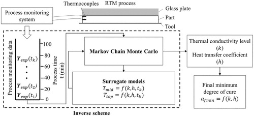
The inversion procedure has been set up to run in parallel with the cure process estimating in real time the thermal properties, boundary conditions and minimum final degree of cure as illustrated in Figure 3. The inverse analysis starts when the first process monitoring data arrive and uses this information to predict the thermal properties $\text{k}$ and $\text{h}$, and consequently the minimum final degree of cure in real time. The inversion scheme uses the MCMC method. The inversion scheme uses the MCMC method. MCMC is executed providing probabilistic estimations in real time, while the monitoring matrix ${\mathbf{\text{Y}}}_{\mathbf{\text{exp}}}\left(\text{t}\right)\in {\mathbb{R}}^{{\mathbf{\text{N}}}_{\mathbf{\text{k}}}\text{x}2}$ is being updated with new data batch every minute. The MCMC links the experimental data – in this case temperatures at mid-thickness and on the top of the composite part at the time ${\text{t}}_{\mathrm{k}}$ with the corresponding surrogate model responses ${\mathbf{\text{Y}}}_{\mathbf{\text{T}}}=\left[{\mathbf{\text{Y}}}_1,{\mathbf{\text{Y}}}_2\right],{\mathbf{\text{Y}}}_{\mathbf{\text{T}}}\in {\mathbb{R}}^{{\mathbf{\text{N}}}_{\mathbf{\text{k}}}\text{x}2}$ through the proportional form of Bayes’ theorem: (24) $\mathrm{P}\left({\mathbf{\text{Y}}}_{\mathbf{\text{T}}}\text{|}{\mathbf{\text{Y}}}_{\mathbf{\text{exp}}}\right)=\frac{\mathrm{P}\left({\mathbf{\text{Y}}}_{\mathbf{\text{exp}}}\text{|}{\mathbf{\text{Y}}}_{\mathbf{\text{T}}}\right)\mathrm{P}\left({\mathbf{\text{Y}}}_{\mathbf{\text{T}}}\right)}{\mathrm{P}\left({\mathbf{\text{Y}}}_{\mathbf{\text{exp}}}\right)}$(24) where $\text{P}\left({\mathbf{\text{Y}}}_{\mathbf{\text{T}}}\text{|}{\mathbf{\text{Y}}}_{\mathbf{\text{exp}}}\right)$ is the posterior probability density function, $\text{P}\left({\mathbf{\text{Y}}}_{\mathbf{\text{exp}}}\text{|}{\mathbf{\text{Y}}}_{\mathbf{\text{T}}}\right)$ the likelihood density function, $\text{P}\left({\mathbf{\text{Y}}}_{\mathbf{\text{T}}}\right)$ the prior density function and $\text{P}\left({\mathbf{\text{Y}}}_{\mathbf{\text{exp}}}\right)$ the normalization constant. Bayes’ theorem can be expressed in a proportional form, where the posterior probability depends on the likelihood and prior distribution as follows: (25) $\text{P}\left({\mathbf{\text{Y}}}_{\mathbf{\text{T}}}\text{|}{\mathbf{\text{Y}}}_{\mathbf{\text{exp}}}\right)\propto \text{P}\left({\mathbf{\text{Y}}}_{\mathbf{\text{exp}}}\text{|}{\mathbf{\text{Y}}}_{\mathbf{\text{T}}}\right)\text{P}\left({\mathbf{\text{Y}}}_{\mathbf{\text{T}}}\right)$(25) The Metropolis Hasting (MH) algorithm was utilized to implement the MCMC. The MH algorithm generates samples ${\mathbf{\text{V}}}_{\mathbf{\text{j}}}=\left[\text{k},\text{h}\right],{\mathbf{\text{V}}}_{\mathbf{\text{j}}}\in {\mathbb{R}}^2$ from a proposal distribution $\text{ q}\left({\mathbf{\text{V}}}_{\mathbf{\text{j}}}|{\mathbf{\text{V}}}_{\mathbf{\text{j}}-1}\right)$. An acceptance criterion is applied in each proposed sample and by accepting or rejecting it, the posterior distribution converges to the target distribution $\text{ P}\left({\mathbf{\text{Y}}}_{\mathbf{\text{T}}}\left({\mathbf{\text{V}}}_{\mathbf{\text{j}}},{\text{t}}_{\mathrm{k}}\right)\text{|}{\mathbf{\text{Y}}}_{\mathbf{\text{exp}}}\left({\text{t}}_{\mathrm{k}}\right)\right)$. Here, ${\mathbf{\text{V}}}_{\mathbf{\text{j}}}$ is a vector representing the unknown parameters $\text{k }$ and $\text{h }$ used to compute the model response ${\mathbf{\text{Y}}}_{\mathbf{\text{T}}}\left({\mathbf{\text{V}}}_{\mathbf{\text{j}}},{\text{t}}_{\mathrm{k}}\right)$ at time ${\text{t}}_{\mathrm{k}}$. The acceptance criterion is expressed as (26) $\alpha =\text{min}\left\{1,\frac{\text{ P}\left({\mathbf{\text{Y}}}_{\mathbf{\text{T}}}\left({\mathbf{\text{V}}}_{\mathbf{\text{j}}},{\text{t}}_{\mathrm{k}}\right)\text{|}{\mathbf{\text{Y}}}_{\mathbf{\text{exp}}}\left({\text{t}}_{\mathrm{k}}\right)\right)\cdot \text{q}\left({\mathbf{\text{V}}}_{\mathbf{\text{j}}}|{\mathbf{\text{V}}}_{\mathbf{\text{j}}-1}\right)}{\text{ P}\left({\mathbf{\text{Y}}}_{\mathbf{\text{T}}}\left({\mathbf{\text{V}}}_{\mathbf{\text{j}}-1},{\text{t}}_{\mathrm{k}}\right)\text{|}{\mathbf{\text{Y}}}_{\mathbf{\text{exp}}}\left({\text{t}}_{\mathrm{k}}\right)\right)\cdot \text{q}\left({\mathbf{\text{V}}}_{\mathbf{\text{j}}-1}|{\mathbf{\text{V}}}_{\mathbf{\text{j}}}\right)}\right\}$(26) where ${\mathbf{\text{V}}}_{\mathbf{\text{j}}}$ and ${\mathbf{\text{V}}}_{\mathbf{\text{j}}-1}$ are the samples of MCMC at iterations $\text{j}$ and $\text{j}-1$, respectively.

Figure 3. Real-time uncertainty estimation framework.

The random walk MH algorithm, which is a modification of the conventional MH, was implemented in this study. In this method the proposal distribution $\text{q}(\cdot )$ is symmetric and can be eliminated from Equation (26). The new sample ${\mathbf{\text{V}}}_{\mathbf{\text{j}}}$ can be calculated incrementally using a Gaussian variable $\text{ε}=\left[{\text{ε}}_{\mathrm{k}},{\text{ε}}_{\mathrm{h}}\right],\text{ε}\in {\mathbb{R}}^2$ with mean value 0 and standard deviation ${\text{σ}}_{\text{ε}}=\left[{{\text{σ}}_{\text{ε}}}_{\mathrm{k}},{{\text{σ}}_{\text{ε}}}_{\mathrm{h}}\right],{\text{σ}}_{\text{ε}}\in {\mathbb{R}}^2$, which is applied to the parameter value ${\mathbf{\text{V}}}_{\mathbf{\text{j}}-1}$ from the previous step. The algorithm operates in the following steps:

1. Initialize ${\mathbf{\text{V}}}_0=\left[{\text{k}}_0,{\text{h}}_0\right]$

2. For $\text{j}=1$ to $\text{M}$ do

   1. Draw a sample $\text{u}\sim \text{U}\left(0,1\right)$ from a uniform distribution.

   2. Draw sample $\text{ε}\sim \mathrm{N}\left(0,{\text{σ}}_{\text{ε}}\right)\to {\mathbf{\text{V}}}_{\mathbf{\text{j}}}={\mathbf{\text{V}}}_{\mathbf{\text{j}}-1}+\text{ε}$

   3. Calculate acceptance probability $\alpha$

   4. If $\text{u}\le \alpha$ then accept ${\mathbf{\text{V}}}_{\mathbf{\text{j}}}$

   5. Else go to step 2 with ${\mathbf{\text{V}}}_{\mathbf{\text{j}}}={\mathbf{\text{V}}}_{\mathbf{\text{j}}-1}$

In this algorithm $M$ is the number of MCMC iterations, and $\alpha$ can be rewritten as follows: (27) $\alpha =\text{min}\left\{1,\frac{\text{ P}\left({\mathbf{\text{Y}}}_{\mathbf{\text{T}}}\left({\mathbf{\text{V}}}_{\mathbf{\text{j}}},{\text{t}}_{\mathrm{k}}\right)\text{|}{\mathbf{\text{Y}}}_{\mathbf{\text{exp}}}\left({\text{t}}_{\mathrm{k}}\right)\right)}{\text{ P}\left({\mathbf{\text{Y}}}_{\mathbf{\text{T}}}\left({\mathbf{\text{V}}}_{\mathbf{\text{j}}-1},{\text{t}}_{\mathrm{k}}\right)\text{|}{\mathbf{\text{Y}}}_{\mathbf{\text{exp}}}\left({\text{t}}_{\mathrm{k}}\right)\right)}\right\}$(27) The posterior probability in Equation (27) can be calculated using Equation (25) and the acceptance probability becomes: (28) $\alpha =\text{min}\left\{1,\frac{\text{ P}\left({\mathbf{\text{Y}}}_{\mathbf{\text{exp}}}\left({\text{t}}_{\mathrm{k}}\right)\text{|}{\mathbf{\text{Y}}}_{\mathbf{\text{T}}}\left({\mathbf{\text{V}}}_{\mathbf{\text{j}}},{\text{t}}_{\mathrm{k}}\right)\right)\text{P}\left({\mathbf{\text{V}}}_{\mathbf{\text{j}}}\right)}{\text{ P}\left({\mathbf{\text{Y}}}_{\mathbf{\text{exp}}}\left({\text{t}}_{\mathrm{k}}\right)\text{|}{\mathbf{\text{Y}}}_{\mathbf{\text{T}}}\left({\mathbf{\text{V}}}_{\mathbf{\text{j}}-1},{\text{t}}_{\mathrm{k}}\right)\right)\text{P}\left({\mathbf{\text{V}}}_{\mathbf{\text{j}}-1}\right)}\right\}$(28) The likelihood term can be expressed as follows: (29) $\text{P}\left({\mathbf{\text{Y}}}_{\mathbf{\text{exp}}}\left({\text{t}}_{\mathrm{k}}\right)\text{|}{\mathbf{\text{Y}}}_{\mathbf{\text{T}}}\left({\mathbf{\text{V}}}_{\mathbf{\text{j}}},{\text{t}}_{\mathrm{k}}\right)\right)=\prod _{\text{k}=1}^{{\text{N}}_{\mathrm{k}}}\text{N}\left({\mathbf{\text{Y}}}_{\mathbf{\text{exp}}}\left({\text{t}}_{\mathrm{k}}\right);{\mathbf{\text{Y}}}_{\mathbf{\text{T}}}\left({\mathbf{\text{X}}}_{\mathbf{\text{j}}},{\text{t}}_{\mathrm{k}}\right),\text{σ}\right)$(29) where ${\text{N}}_{\mathrm{k}}$ denotes the number of experimental data available at time ${\text{t}}_{\mathrm{k}}$. The likelihood incorporates all the distributions which are computed with experimental data ${\mathbf{\text{Y}}}_{\mathbf{\text{exp}}}$ using a normal distribution with the model values ${\mathbf{\text{Y}}}_{\mathbf{\text{T}}}\left({\mathbf{\text{V}}}_{\mathbf{\text{j}}},{\text{t}}_{\mathrm{k}}\right)$ as a mean and a standard deviation $\text{σ}$. The prior distribution is computed in a similar way as (30) $\text{P}\left({\mathbf{\text{V}}}_{\mathbf{\text{j}}}\right)=\prod _{\text{o}=1}^{{\text{n}}_{\mathrm{p}}}\text{N}\left({\text{V}}_{\mathrm{j}}^{\text{o}};{\text{μ}}_{\text{prior}}^{\text{o}},{\text{σ}}_{\text{prior}}^{\text{o}}\right)$(30) where $n_p$ is the number of unknown parameters ($k$ and h), whilst ${\text{μ}}_{\mathbf{\text{prior}}}=\left[{\text{μ}}_{\text{prior}}^{\text{k}},{\text{μ}}_{\text{prior}}^{\text{h}}\right],{\text{μ}}_{\mathbf{\text{prior}}}\in {\mathbb{R}}^2$ and ${\text{σ}}_{\mathbf{\text{prior}}}=\left[{\text{σ}}_{\text{prior}}^{\text{k}},{\text{σ}}_{\text{prior}}^{\text{h}}\right],{\text{σ}}_{\mathbf{\text{prior}}}\in {\mathbb{R}}^2$ are the mean and standard deviation of the prior distributions. The first and second statistical moments of the prior distribution of $\text{h}$ and k were selected based on the results of uncertainty quantification experiments [3] and on the experimental scatter [23] and are summarized in Table 4.

The standard deviation $\text{σ}$ used in the likelihood term represents the accuracy level of experimental data and is assigned with a small value taking into account the low noise levels of thermocouple signals. In the case of K-type thermocouples, the error can reach up to 2°C [24]. In the MCMC algorithm, standard deviations ${\text{σ}}_{\text{ε}}$ operate as tuning parameters and need to be adjusted before the initiation of the inversion procedure. The standard deviation vector ${\text{σ}}_{\text{ε}}$ determines the sampling behaviour of the chain [25]. The right choice of these standard deviations depends on the acceptance probability rate which must be between 15% and 50% for low-dimensionality models achieving a good mixing behaviour of the sequence [26] and need to be tuned when the experimental matrix is updated with new data. A short sequence of MCMC iterations was performed every minute after acquisition of the new data set to tune the standard deviation vector ${\text{σ}}_{\text{ε}}$ to achieve the desirable acceptance probability. The initial noise level standard deviation was set equal to standard deviation of the prior distributions. The standard deviation values are reported in Table 4.

Simulations of a single chain may be trapped in a local mode failing to explore modes with notable probability. A similar phenomenon is pronounced in a gradient-based solution when the algorithm is trapped in local minimum in non-linear model fitting. Parallel tempering was applied to address this problem combining the simulated annealing method [27] with the use of parallel chains [28]. In this method a temperature parameter $T_{\text{pt}}$ with the property $1\le T_{\text{pt}}\le \mathrm{\infty }$ is introduced, where $T_{\text{pt}}=1$ corresponds to the desired target distribution and is referred to as a cold sample [29]. Values with $T_{\text{pt}}\gg 1$, which are referred to as hot samples, flatten the target distribution and allow the acceptance of a wider range of proposed parameters. Hence, these distributions explore a larger parameter region and thus are less likely to be trapped in local modes. In parallel tempering, a parameter defined as $\text{ z}=1/T_{\text{pt}}$ is assigned to the likelihood term as follows: (31) $\pi \left({\mathbf{\text{Y}}}_{\mathbf{\text{T}}}\left({\mathbf{\text{X}}}_{\mathbf{\text{j}}},\text{t}\right)\text{|}{\mathbf{\text{Y}}}_{\mathbf{\text{exp}}}\left(\text{t}\right),\text{w}\right)=\text{P}({\mathbf{\text{Y}}}_{\mathbf{\text{exp}}}\left(\text{t}\right)\text{|}{\mathbf{\text{Y}}}_{\mathbf{\text{T}}}\left({\mathbf{\text{X}}}_{\mathbf{\text{j}}},\text{t}\right){)}^{\text{z}}\text{P}\left({\mathbf{\text{X}}}_{\mathbf{\text{j}}}\right)\text{for }0<\text{z}<1$(31) This tempering posterior distribution is calculated using Equation (25). A different discrete value of $\text{z}$ is assigned in each of the ${\text{n}}_{\text{ch}}$ chains resulting in a ladder with different temperatures. After a certain number of iterations $\left({\text{n}}_{\mathrm{s}}\right)$, a parameter swap algorithm is initiated which exchanges parameters between two chains, if ${\text{U}}_1\sim \text{U}\left[0,1\right]\le 1/n_{\mathrm{s}}$ with ${\text{U}}_1$ being a random number drawn from a uniform distribution. If the swap occurs, a chain $\text{l }$ is randomly selected to swap the parameter set with the chain $\text{ l}+1$. A swap is accepted if $\text{s}\ge {\text{U}}_2$ where ${\text{U}}_2\sim \text{U}\left[0,1\right]$ and ${\alpha }_{\text{pt}}$ is the acceptancess probability expressed as (32) ${\alpha }_{\text{pt}}=\text{min}\left\{1,\frac{\pi \left({\mathbf{\text{Y}}}_{\mathbf{\text{T}}}\left({\mathbf{\text{X}}}_{\mathbf{\text{j}}}^{\mathbf{\text{l}}+1},\text{t}\right)\text{|}{\mathbf{\text{Y}}}_{\mathbf{\text{exp}}}\left(\text{t}\right),{\text{z}}_{\mathrm{l}}\right)\pi \left({\mathbf{\text{Y}}}_{\mathbf{\text{T}}}\left({\mathbf{\text{X}}}_{\mathbf{\text{j}}}^{\mathbf{\text{l}}},\text{t}\right)\text{|}{\mathbf{\text{Y}}}_{\mathbf{\text{exp}}}\left(\text{t}\right),{\text{z}}_{\text{l}+1}\right)}{\pi \left({\mathbf{\text{Y}}}_{\mathbf{\text{T}}}\left({\mathbf{\text{X}}}_{\mathbf{\text{j}}}^{\mathbf{\text{l}}},\text{t}\right)\text{|}{\mathbf{\text{Y}}}_{\mathbf{\text{exp}}}\left(\text{t}\right),{\text{z}}_{\mathrm{l}}\right)\pi \left({\mathbf{\text{Y}}}_{\mathbf{\text{T}}}\left({\mathbf{\text{X}}}_{\mathbf{\text{j}}}^{\mathbf{\text{l}}+1},\text{t}\right)\text{|}{\mathbf{\text{Y}}}_{\mathbf{\text{exp}}}\left(\text{t}\right),{\text{z}}_{\text{l}+1}\right)}\right\}$(32) Chains with higher temperatures can explore different modes, whilst chains within the ladder allow the possibility to refine these sets. Only the results of the cold chain corresponding to the target distribution are considered for the final sample, whilst the results from the remaining chains are disregarded [30].

The number of MCMC iterations in real time depends on the execution time of one iteration. The execution time increases with increasing experimental data. In the beginning of the process for a given high specification personal computer (4 cores @3.2 GHz), the rate of MCMC iterations was about 20,000 per minute, whilst towards the end of the process the rate decreased to about 500 iterations per minute. The total MCMC iterations of the inversion procedure were approximately 210,000. Table 4 reports the MH algorithm parameter values.

3. Results and discussion

3.1. Validation of the surrogate model

Response surfaces, expressing the relationship between models outputs and inputs, were constructed to compare the surrogate model with the FE model results. The surrogate models were tested using inputs points within the whole range of the design space different from the sample points used for their construction. Figure 4(a,b) illustrate the dependence of model outputs ($T_{\text{mid}},T_{\text{top}}$) on inputs ($k$ and $h$) at 60 min in the cure process. It can be observed that the heat transfer coefficient causes greater changes in $T_{\text{mid}}$ and $T_{\text{top}}$ than the thermal conductivity level. This is attributed to the fact that the response surface corresponds to a time at which the tool temperature has reached a plateau and the thermal conductivity level effect has been reduced. The temperature at the top of the part is more sensitive to parameter changes than the temperature at mid-thickness. The temperature is reduced when the surface heat transfer coefficient increases and the thermal conductivity level decreases. Figure 4(c) illustrates the relationship of the minimum final degree of cure with the underlying parameters of the surrogate model. The minimum final conversion decreases with increasing surface heat transfer coefficient and decreasing thermal conductivity level. A pronounced steep decrease of the final degree of cure occurs when the thermal conductivity level is in the range between 0.01 and 0.05 W/m/°C. In this area, the minimum final conversion reaches values as low as 0.7.

Figure 4. Response surfaces (a) temperature at mid-thickness as a function of the heat transfer coefficient and the thermal conductivity level at 60 min; (b) temperature on the top as a function of the heat transfer coefficient and the thermal conductivity level at 60 min and (c) minimum final degree of cure as a function of the heat transfer coefficient and the thermal conductivity level.

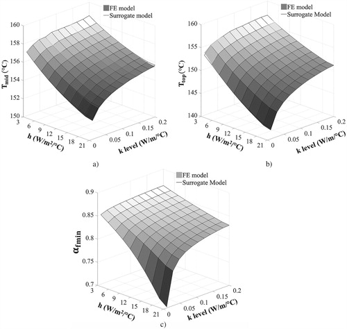
The three surrogate models are in very close agreement with the FE model with the average absolute difference being equal to 0.2°C for the first and second surrogate models estimated ($T_{\text{mid}},T_{\text{top}}$) and 3 × 10⁻⁶ for the third model corresponding to the minimum final degree of cure. The discrepancy between the FE and surrogate model does not affect the predictions’ fidelity of the inversion scheme since the corresponding error of surrogate models (0.2°C) is significantly lower than the standard deviation $\text{σ}$ which screens K-type thermocouples’ experimental error. The surrogate model execution time is approximately 4 ms on the 4 cores @3.2 GHz computer used, whilst the FE model takes 30 s to solve the cure problem. This difference in execution times which reached about 4 orders of magnitude highlights the efficiency of the surrogate model on estimating cure models’ outputs within the input domain, whilst the very short computation required for the surrogate model allows its utilization in real-time computational processing.

3.2. Real-time estimation

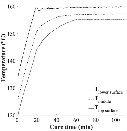
Figure 5 illustrates the process monitoring results obtained during the cure; the temperature evolution with cure time at the lower surface, at mid-thickness and on the top of the curing composite. It can be observed that the temperature is lower away from the heated tool surface reaching a plateau after 60 min from the beginning of the cure process. Temperature overshoots due to the exothermic nature of the resin reaction are not detected due to the small thickness of the composite part. Measurement noise is negligibly located on the shoulder and on the slope of the temperature of the lower surface and mid-thickness, respectively.

Figure 5. Process monitoring data.

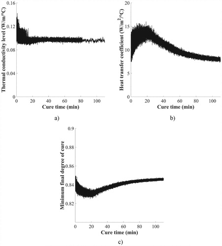
Figure 6 illustrates the evolution of thermal conductivity level, surface heat transfer coefficient and minimum final conversion of the cold chain during the process. The thermal conductivity level converges faster than the surface heat transfer coefficient reaching a plateau after 20 min in the cure. This can be attributed to the fact that in the first 20 min the tool temperature increases, and transient phenomena governed by thermal conductivity dominate the evolution of the thermal field. The surface heat transfer coefficient and minimum final degree of cure converge after 70 min as depicted in Figures 6(b,c), presenting a step decrease/increase pattern as a result of the periodic updating of monitoring data. At about 70 min the top surface temperature reaches a plateau of 155°C and the thermal response becomes more sensitive to the surface heat transfer coefficient.

Figure 6. Real-time evolution of estimated variables: (a) thermal conductivity level; (b) surface heat transfer coefficient and (c) minimum final degree of cure.

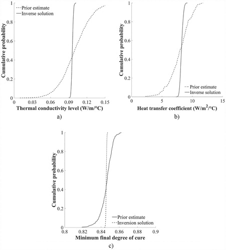
The sample after convergence can be used to calculate the statistical properties of variables of interest. The values within the stationary sequence are highly correlated due to the nature of the MH algorithm. Consequently, a step size calculated considering the autocorrelation structure of the initial sampling of thermal conductivity level, surface heat transfer coefficient and minimum final conversion was used for thinning the sample. Figure 7(a–c) depicts the prior estimate and inversion solution cumulative probabilities of the thermal conductivity level, heat transfer coefficient and minimum final degree of cure, respectively. The mean value of thermal conductivity level is 0.095 W/m/°C, which is relatively close to the prior mean value of 0.12 W/m/°C, whilst the standard deviation is very low and equal to 0.002 W/m/°C. The heat transfer coefficient average is 8.2 W/m²/°C with a standard deviation of 0.2 W/m²/°C, whereas the nominal value is 8.5 W/m²/°C. In terms of variability, the inversion procedure reduces the estimation uncertainty of the surface heat transfer coefficient lowering its coefficient of variation from 18% [2] to 3%. In the case of the estimated minimum final degree of cure, the mean value is 0.845 with a standard deviation of 7 × 10⁻⁴ resulting in a 0.08% coefficient of variation. A Monte Carlo simulation has been carried out using the prior statistical properties of the unknown stochastic variables to estimate the minimum final degree of cure without the information acquired from the process monitoring system. Prior estimates result in a wide range of minimum final conversion values from 0.82 to 0.86. This uncertainty may result in variations of final glass transition temperature potentially affecting high temperature performance. The estimated minimum final degree of cure variability was reduced by 90% as a result of the inversion procedure. The low uncertainty prediction of the minimum final conversion during the curing stage allows control decisions to be made preventing undesirable effects such as undercure.

Figure 7. Cumulative probabilities before and after inverse analysis: (a) thermal conductivity level; (b) heat transfer coefficient and (c) minimum final degree of cure.

Figure 8(a) illustrates the experimental measurements results on the lower surface, the mid-thickness and the top of the curing part alongside the 95% confidence intervals of model response estimated using the prior statistical properties of the thermal conductivity level and surface heat transfer coefficient (Table 4). The confidence intervals of prior model estimations are wide, highlighting the influence of stochastic variables on the through thickness temperature distribution. These results indicate the benefits of estimating the resin thermal conductivity level and surface heat transfer coefficient from the real-time experimental data. After inverse analysis the confidence intervals are narrowed down, and the model approximations of measured temperatures calculated with the estimated mean values of unknown variables are in close agreement with the experimental data with an average error of 1°C (Figure 8(b)). The relatively small discrepancies between experimental data and final model predictions are attributed to a compromise of the inversion procedure on the estimation of unknown parameters in order to address the unexpected phenomena that had occurred during the manufacturing process. The capability of the inversion procedure to run simultaneously with the manufacturing process enables accurate predictions in real time of the process outcomes by updating the cure model with the upcoming monitoring data.

Figure 8. Experimental data and probabilistic model response comparison: (a) prior knowledge; (b) estimated values; (c) evolution of minimum degree of cure and 99% confidence intervals of estimated minimum final degree of cure with time and (d) 99% confidence intervals of the estimated minimum final glass transient temperature with time.

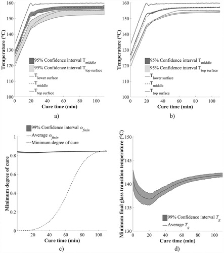
Figure 8(c,d) depicts the evolution of the 99% confidence intervals of the minimum final degree of cure estimation and actual minimum degree of cure with time and the corresponding results for the evolution of the final minimum predicted glass transition temperature. The evolution of the actual minimum degree of cure was calculated using a non-parametric cure kinetics model considering as an input the top surface temperature evolution with time [31] and the glass transition temperature based on Equation (5). The comparison of the predicted with the actual minimum final conversion indicates the estimation capabilities of the cure model during the inversion scheme. The estimated error is approximately 0.9%. The final glass transition estimate involves uncertainty of about 4°C. This is reduced as result of taking into account the monitoring data to about 1°C. This, as well as potential correction of glass transition temperature levels using monitoring data, can have a significant implication in the high temperature performance of the produced composite. The overall scheme allows the continuous updating with new monitoring data sets enhancing cure model fidelity on predicting the unknown parameters and consequently the desirable process outcomes with low uncertainty.

4. Conclusions

An inversion procedure based on MCMC was developed in this study to estimate in real time the uncertainty and the evolution of the curing stage of the manufacturing of composite materials. The utilization of a surrogate model significantly reduces the computational time whilst representing accurately the heat transfer problem. The developed inversion methodology overcomes limitations presented in deterministic approaches, addressing successfully potential ill-posedness of inverse cure problems considering the prior distribution of stochastic variables. The methodology presented in this study is the first comprehensive attempt to integrate process monitoring with process modelling in real time for uncertainty estimation in composites manufacture. The use of fast surrogate models is a major enabler of this approach. The successful online implementation of the inversion procedure eliminates the gap between stochastic simulation and manufacturing process. The findings highlight the effectiveness of the MCMC method in terms of estimating the statistical properties of the resin thermal conductivity level and surface heat transfer coefficient and predicting the process outcomes in real time. The developed scheme predicts with very low uncertainty the minimum final degree of cure with a corresponding error of about 0.9%. This accuracy is translated directly to an accurate estimate of the final glass transition of the material.

The modelling-monitoring integration scheme proposed here can be utilized to reduce the inherent uncertainty of the process and to predict the process outcomes and its uncertainty using the results of process monitoring. This development is a step towards the application of a hybrid twin to the composite manufacturing process. This aims to achieve a prediction of composites processing outcomes in real time using simulation and information acquired from sensors incorporated in the manufacturing assembly. This will allow the implementation of control methodologies based on the probabilistic prediction of process outcome leading to benefits in terms of cost and quality. The same scheme can be used to assess quality in real time during processing, minimizing the resources required for post-production inspection.

Acknowledgements

Data underlying this study can be accessed through the Cranfield University repository at: https://doi.org/10.17862/cranfield.rd.5706007.

Disclosure statement

No potential conflict of interest was reported by the authors.

Additional information

Funding

This work was supported by EU through the Clean Sky 2 project SimCoDeQ (project ID: 686493) Engineering and Physical Sciences Research Council through the grant ‘Robustness performance optimisation for automated composites manufacture’ [grant number EP/K031430/1] and H2020 Societal Challenges [grant number 686493].

References

- Mesogitis TS, Skordos AA, Long AC. Uncertainty in the manufacturing of fibrous thermosetting composites: a review. Compos Part A Appl Sci Manuf. 2014;57(2):67–75. doi: 10.1016/j.compositesa.2013.11.004
- Tifkitsis KI, Mesogitis TS, Struzziero G, et al. Stochastic multi-objective optimisation of the cure process of thick laminates. Compos Part A. 2018;112(9):383–394. doi: 10.1016/j.compositesa.2018.06.015
- Mesogitis TS, Skordos AA, Long AC. Stochastic heat transfer simulation of the cure of advanced composites. J Compos Mater. 2016;50(21):2971–2986. doi: 10.1177/0021998315615200
- Mesogitis TS, Skordos AA, Long AC. Stochastic simulation of the influence of cure kinetics uncertainty on composites cure. Compos Sci Technol. 2015;110(4):145–151. doi: 10.1016/j.compscitech.2015.02.009
- Maistros GM, Partridge IK. Monitoring autoclave cure in commercial carbon fibre/epoxy composites. Compos Part B Eng. 1998;29(3):245–250. doi: 10.1016/S1359-8368(97)00020-6
- Di Fratta C, Klunker F, Trochu F, et al. Characterization of textile permeability as a function of fiber volume content with a single unidirectional injection experiment. Compos Part A Appl Sci Manuf. 2015;77(10):238–247. doi: 10.1016/j.compositesa.2015.05.021
- Konstantopoulos S, Grössing H, Patrick H, et al. Determination of the unsaturated through-thickness permeability of fibrous preforms based on flow front detection by ultrasound. Polym Compos. 2018;39(2):360–367. doi: 10.1002/pc.23944
- Bai-Jian W, Yu-Sung C, Yuan Y, et al. Online estimation and monitoring of local permeability in resin transfer molding. Polym Compos. 2016;37(4):1249–1258. doi: 10.1002/pc.23290
- Skordos AA, Partridge IK. Inverse heat transfer for optimization and on-line thermal properties estimation in composites curing. Inverse Probl Sci Eng. 2004;12(2):157–172. doi: 10.1080/10682760310001598616
- Xiong XT, Shi WX, Hon YC. A one-dimensional inverse problem in composite materials: regularization and error estimates. Appl Math Model. 2015;39(18):5480–5494. doi: 10.1016/j.apm.2015.01.004
- Wang J, Zabaras N. Using Bayesian statistics in the estimation of heat source in radiation. Int J Heat Mass Transf. 2005;48(1):15–29. doi: 10.1016/j.ijheatmasstransfer.2004.08.009
- Wang J, Zabaras N. A Bayesian inference approach to the inverse heat conduction problem. Int J Heat Mass Transf. 2004;47(17):3927–3941. doi: 10.1016/j.ijheatmasstransfer.2004.02.028
- Kaipio JP, Fox C. The Bayesian framework for inverse problems in heat transfer. Heat Transf Eng. 2011;32(9):718–753. doi: 10.1080/01457632.2011.525137
- “TohoTenax, Delivery programme and characteristics Tenax HTA filament yarn, Toho Tenax Europe GmbH.” 2011.
- “Hexcel HexFlow® RTM6 epoxy system for Resin Transfer Moulding Monocomponent system Product Data. www.hexcel.com.” 2018.
- “Marc® volume B: Element library.” 2018.
- “Marc® volume D: User subroutines and Special Routines.” 2018.
- Karkanas PI, Partridge IK. Cure modeling and monitoring of epoxy/amine resin systems. I. Cure kinetics modeling. J Appl Polym Sci. 2000;77(7):1419–1431. doi: 10.1002/1097-4628(20000815)77:7<1419::AID-APP3>3.0.CO;2-N
- Pascault JP, Williams RJJ. Relationships between glass transition temperature and conversion. Polym Bull. Jul. 1990;24(1):115–121. doi: 10.1007/BF00298330
- Farmer JD, Covert EE. Thermal conductivity of a thermosetting advanced composite during its cure. J Thermophys Heat Transf. 1996;10(3):467–475. doi: 10.2514/3.812
- Struzziero G, Skordos AA. Multi-objective optimisation of the cure of thick components. Compos Part A Appl Sci Manuf. 2017;93(2):126–136. doi: 10.1016/j.compositesa.2016.11.014
- Lophaven SN, Nielsen HB, Søndergaard J. “DACE-A Matlab Kriging toolbox, version 2.0.” 2002.
- Struzziero G, Remy B, Skordos AA. Measurement of thermal conductivity of epoxy resins during cure. J Appl Polym Sci. 2018;47015(8):1–10.
- Kollie TG, Horton JL, Carr KR, et al. Temperature measurement errors with type K (Chromel vs Alumel) thermocouples due to short-ranged ordering in Chromel. Rev Sci Instrum. 1975;46(11):1447–1461. doi: 10.1063/1.1134086
- Roberts GO, Gelman A, Gilks WR. Weak convergence and optimal scaling of random walk Metropolis algorithms. Ann Appl Probab. 1997;7(1):110–120. doi: 10.1214/aoap/1034625254
- Roberts GO, Rosenthal JS, Schwartz PO. Convergence properties of perturbed Markov chains. J Appl Probab. 1998;35(1):1–11. doi: 10.1239/jap/1032192546
- Kirkpatrick S, Gelatt CD, Vecchi MP. Optimization by simulated annealing. Science (80). 1983;220(4598):671–680. doi: 10.1126/science.220.4598.671
- Swendsen RH, Wang J-S. Replica Monte Carlo simulation of spin-glasses. Phys Rev Lett. 1986;57(21):2607–2609. doi: 10.1103/PhysRevLett.57.2607
- Geyer CJ, Thompson EA. Annealing Markov chain Monte Carlo with applications to ancestral inference. J Am Stat Assoc. 1995;90(431):909–920. doi: 10.1080/01621459.1995.10476590
- Gregory P. Bayesian logical data analysis for the physical sciences: a comparative approach with Mathematica® Support. Cambridge: Cambridge University Press; 2005.
- Skordos AA, Partridge IK. Cure kinetics modeling of epoxy resins using a non-parametric numericaI procedure. Polym Eng Sci. 2001;41(5):793–805. doi: 10.1002/pen.10777