Solving a nonlinear inverse Sturm–Liouville problem with nonlinear convective term using a boundary functional method

Abstract

This article is concerned with solving nonlinear inverse problems to recover the second-order nonlinear Sturm–Liouville operators, probably including a nonlinear convective term, which refers to over-specified boundary data. Utilising a homogenization approach with the boundary data, a series of boundary functions are obtained and consist of a linear space combined with the zero element. The energetic functional both qualifying the homogeneous boundary conditions and maintaining the energy is presented in the linear space based on the energetic boundary functions. The multiplier can be decided by solving a nonlinear equation. The linear systems utilized in rebuilding the uncertain leading coefficient function as well as the potential function in the nonlinear Sturm–Liouville operator are improved, so that the iterative algorithms converge rapidly. Numerical examples provided indicate that the presented method is well capable of recovering the nonlinear Sturm–Liouville operators with a nonlinear convective term.

Keywords:

• Inverse nonlinear Sturm–Liouville operator
• inverse coefficient problem
• potential function
• boundary functional method
• inverse problems

2010 Mathematics Subject Classification:

• 31B20

1. Introduction

The inverse Sturm–Liouville problem has been applied widely in research and industrial applications such as the identification of mechanical characteristics and geometry of vibrating continuum; however, it remains difficult to find either a theoretical solution or a numerical solution to the problem. The potential function uniquely decided by the spectral function was initially established by Gelfand and Levitan [1]. Following this, an analytical method adapting the process to the inverse Sturm–Liouville problem was given by McLaughlin [2]. Bondarenko et al. [3] set up a procedure for recovering the Sturm–Liouville operators of the inverse problem from the spectrum. Sat et al. [4] rebuilt the singular Sturm–Liouville operator from one spectrum and some eigenfunctions at the internal point.

The problem, referred to as the inverse spectral problem or inverse eigenvalue problem [5], was constituted by many techniques for solving the linear inverse Sturm–Liouville problem to rebuild the potential function according to specified eigenvalues [6,7]. In addition, it was McLaughlin [8] that primarily presented the possibility of acquiring the potential function and boundary conditions through the set of nodal points, which was called the inverse nodal problem [9–12]. Sat et al. [13] investigated the inverse nodal problems for Sturm–Liouville- type integrodifferential operators with a constant delay.

Although the inverse Sturm–Liouville problem can be converted into an inverse eigenvalue problem of a settled matrix [14] by means of numerical methods, the inverse algorithms built on discretisations require an elaborative implementation [6,7], because these discretisations in a matrix form with higher eigenvalues are vastly different from those of true eigenvalues.

Consider the linear Sturm–Liouville boundary value problem: (1) $\begin{array}{rl}& -\frac{\mathrm{d}}{\mathrm{d}x}[p(x)\frac{\mathrm{d}w(x)}{\mathrm{d}x}]+q(x)w(x)=\lambda s(x)w(x),0<x<\ell ,\end{array}$(1) (2) $\begin{array}{rl}& w(0)=0,w(\ell )=0.\end{array}$(2) In particular, the leading coefficient function $p(x)$, the potential function $q(x)$ and the weight function $s(x)$ should be ascertained. However, it is an exceedingly ill-posed problem that is unable to reconstruct these functions if the data of $w(x)$ are unknown. Liu [15] and Liu and Atluri [16] have already investigated this type of inverse problem. An inverse Sturm–Liouville problem with some eigenvalues λ and additional over-specified boundary data is the special case that we describe in this article.

An easy-handling mathematical method is proposed to solve the nonlinear inverse Sturm–Liouville problem: (3) $-[\alpha (x)w^{\mathrm{\prime }}(x){]}^{\mathrm{\prime }}+q(x)F(w(x))=H(x),x\in (0,\ell ),$(3) in which $F(w)$ is a nonlinear function of w. There are four categories of inverse problems of (a) determining the leading coefficient $\alpha (x)$, (b) ascertaining the potential function $q(x)$, (c) reconstructing the unknown function $F(w)$ and (d) ascertaining the forcing term $H(x)$. This article focuses on topics (a) and (b). Primarily supposing that $F(w)=w$, a linear inverse Sturm–Liouville problem arises. In addition, with $H=\lambda s(x)w(x)$ and λ, $s(x)$ and $\alpha (x)$ offered, the potential function $q(x)$ should be reconstructed, which is a particular case discussed in Section 4. The considered inverse problems are highly ill-posed, because much close output data utilized in the determination probably corresponds to extremely different functions.

In addition, the nonlinear inverse Sturm–Liouville problem with a nonlinear convective term is also considered: (4) $-[\alpha (x)w^{\mathrm{\prime }}(x){]}^{\mathrm{\prime }}+q(x)F(w(x))+G(w(x))w^{\mathrm{\prime }}(x)=H(x),x\in (0,\ell ),$(4) in which $G(w(x))w^{\mathrm{\prime }}(x)$ is a nonlinear convective term. A special circumstance of the equation is the steady Burgers problem.

Formulae, an algorithm and numerical computations for topic (a) of Equation (3(3) $-[\alpha (x)w^{\mathrm{\prime }}(x){]}^{\mathrm{\prime }}+q(x)F(w(x))=H(x),x\in (0,\ell ),$(3) ) are introduced; similarly topic (b) of Equation (4(4) $-[\alpha (x)w^{\mathrm{\prime }}(x){]}^{\mathrm{\prime }}+q(x)F(w(x))+G(w(x))w^{\mathrm{\prime }}(x)=H(x),x\in (0,\ell ),$(4) ) is managed, which is deferred to Section 5.

Aiming at handling the inverse problem in topic (a), the boundary data are offered: (5) $\begin{array}{rl}& w(0)=w_0,w(\ell )=w_{\ell },w^{\mathrm{\prime }}(0)=w_0^{\mathrm{\prime }},w^{\mathrm{\prime }}(\ell )=w_{\ell }^{\mathrm{\prime }},\end{array}$(5) (6) $\begin{array}{rl}& \alpha (0)={\alpha }_0,\alpha (\ell )={\alpha }_{\ell },{\alpha }^{\mathrm{\prime }}(0)={\alpha }_0^{\mathrm{\prime }},{\alpha }^{\mathrm{\prime }}(\ell )={\alpha }_{\ell }^{\mathrm{\prime }}.\end{array}$(6) The inverse problem to identify the leading coefficient of the linear Sturm–Liouville equation was investigated by Hasanov and Shores [17], and numerical techniques have been improved through the work of Kaltenbacher [18], Hasanov and Pektas [19], Hasanov [20], as well as Liu [21].

The present article is organized as follows. In Section 2, the original idea of an energy functional is proposed based on energetic boundary functions. It consists of a linear space of polynomial functions, which is not less than fourth order as well as qualifying the over-specified boundary conditions. In Section 3, an iterative algorithm is adopted in determining the unclear leading coefficient function $\alpha (x)$ with three numerical instances provided. In Section 4, similarly to Section 3, with four numerical instances offered, an iterative algorithm is utilized to rebuild the unknown potential function $q(x)$. In Section 5, the algorithms used to determine $\alpha (x)$ and $q(x)$ of Equation (3(3) $-[\alpha (x)w^{\mathrm{\prime }}(x){]}^{\mathrm{\prime }}+q(x)F(w(x))=H(x),x\in (0,\ell ),$(3) ) are adopted to reconstruct $\alpha (x)$ and $q(x)$ of Equation (4(4) $-[\alpha (x)w^{\mathrm{\prime }}(x){]}^{\mathrm{\prime }}+q(x)F(w(x))+G(w(x))w^{\mathrm{\prime }}(x)=H(x),x\in (0,\ell ),$(4) ). Finally, conclusions are drawn in Section 6.

2. An energetic boundary functional approach

First, consider a variable transformation: (7) $y(x)=w(x)-b(x),$(7) in which (8) $b(x)=\frac{1}{{\ell }^3}[2w_0-2w_{\ell }+w_0^{\mathrm{\prime }}\ell +w_{\ell }^{\mathrm{\prime }}\ell ]x^3-\frac{1}{{\ell }^2}[3w_0-3w_{\ell }+2w_0^{\mathrm{\prime }}\ell +w_{\ell }^{\mathrm{\prime }}\ell ]x^2+w_0^{\mathrm{\prime }}x+w_0$(8) is a homogenization function. Based on Equations (3(3) $-[\alpha (x)w^{\mathrm{\prime }}(x){]}^{\mathrm{\prime }}+q(x)F(w(x))=H(x),x\in (0,\ell ),$(3) ) and (5(5) $\begin{array}{rl}& w(0)=w_0,w(\ell )=w_{\ell },w^{\mathrm{\prime }}(0)=w_0^{\mathrm{\prime }},w^{\mathrm{\prime }}(\ell )=w_{\ell }^{\mathrm{\prime }},\end{array}$(5) ) and homogeneous boundary conditions, a new system is derived: (9) $\begin{array}{rl}& -[\alpha (x)(y^{\mathrm{\prime }}(x)+b^{\mathrm{\prime }}(x)){]}^{\mathrm{\prime }}+q(x)F(y(x)+b(x))=H(x),x\in (0,\ell ),\end{array}$(9) (10) $\begin{array}{rl}& y(0)=0,y(\ell )=0,y^{\mathrm{\prime }}(0)=0,y^{\mathrm{\prime }}(\ell )=0.\end{array}$(10) First, multiplying Equation (9(9) $\begin{array}{rl}& -[\alpha (x)(y^{\mathrm{\prime }}(x)+b^{\mathrm{\prime }}(x)){]}^{\mathrm{\prime }}+q(x)F(y(x)+b(x))=H(x),x\in (0,\ell ),\end{array}$(9) ) by $y(x)+b(x)$ and, second, integrating it from x = 0 to $x=\ell$, finally utilizing integration partially and considering Equations (6(6) $\begin{array}{rl}& \alpha (0)={\alpha }_0,\alpha (\ell )={\alpha }_{\ell },{\alpha }^{\mathrm{\prime }}(0)={\alpha }_0^{\mathrm{\prime }},{\alpha }^{\mathrm{\prime }}(\ell )={\alpha }_{\ell }^{\mathrm{\prime }}.\end{array}$(6) ) and (10(10) $\begin{array}{rl}& y(0)=0,y(\ell )=0,y^{\mathrm{\prime }}(0)=0,y^{\mathrm{\prime }}(\ell )=0.\end{array}$(10) ), the energy identity is acquired: (11) $\begin{array}{rl}& {\int }_0^{\ell }\{\alpha (x)[y^{\mathrm{\prime }}(x)+b^{\mathrm{\prime }}(x){]}^2+q(x)Q(y(x)+b(x))-H(x)[y(x)+b(x)]\}\mathrm{d}x\\ & ={\alpha }_{\ell }{w}_{\ell }{w}_{\ell }^{\mathrm{\prime }}-{\alpha }_0{w}_0{w}_0^{\mathrm{\prime }}=:d_0,\end{array}$(11) in which $Q(y(x)+b(x))=(y(x)+b(x))F(y(x)+b(x))$. In conclusion, not only deformation energy but also potential energy and even external work contribute to a constant $d_0$. This equation helps rebuild the leading coefficient function $\alpha (x)$.

In reality, $y(x)$ cannot be precisely obtained in Equations (9(9) $\begin{array}{rl}& -[\alpha (x)(y^{\mathrm{\prime }}(x)+b^{\mathrm{\prime }}(x)){]}^{\mathrm{\prime }}+q(x)F(y(x)+b(x))=H(x),x\in (0,\ell ),\end{array}$(9) ) and (11(11) $\begin{array}{rl}& {\int }_0^{\ell }\{\alpha (x)[y^{\mathrm{\prime }}(x)+b^{\mathrm{\prime }}(x){]}^2+q(x)Q(y(x)+b(x))-H(x)[y(x)+b(x)]\}\mathrm{d}x\\ & ={\alpha }_{\ell }{w}_{\ell }{w}_{\ell }^{\mathrm{\prime }}-{\alpha }_0{w}_0{w}_0^{\mathrm{\prime }}=:d_0,\end{array}$(11) ) owing to the uncertain $\alpha (x)$. Nevertheless, numerous functions are able to be constructed to estimate $y(x)$. Primarily, we obtain the boundary function that naturally qualifies these homogeneous boundary conditions in Equation (10(10) $\begin{array}{rl}& y(0)=0,y(\ell )=0,y^{\mathrm{\prime }}(0)=0,y^{\mathrm{\prime }}(\ell )=0.\end{array}$(10) ): (12) $B_j(x)=(x^4-2\ell x^3+{\ell }^2{x}^2)x^{j-1},j\ge 1,$(12) which are a minimum of fourth-order polynomial functions of x that simultaneously qualify the homogeneous boundary conditions: (13) $B_j(0)=0,B_j(\ell )=0,B_j^{\mathrm{\prime }}(0)=0,B_j^{\mathrm{\prime }}(\ell )=0.$(13) Considering Equations (12(12) $B_j(x)=(x^4-2\ell x^3+{\ell }^2{x}^2)x^{j-1},j\ge 1,$(12) ) and (13(13) $B_j(0)=0,B_j(\ell )=0,B_j^{\mathrm{\prime }}(0)=0,B_j^{\mathrm{\prime }}(\ell )=0.$(13) ), it is apparent that a linear space of boundary functions consists of a sequence of (14) $\{B_j(x)\},j\ge 1$(14) and the zero element enables the combination of $B_j(x)$ to become another boundary function: (15) $E_j(x)={\gamma }_j{B}_j(x)+B_{j+1}(x),j\ge 1,j\text{not summed},$(15) in which ${\gamma }_j$ is a multiplier to be decided later.

The problem becomes determining how to ascertain the multiplier ${\gamma }_j$ for every element of $E_j(x)$. As $E_j(x)$ already conforms to the homogeneous boundary conditions in Equation (10(10) $\begin{array}{rl}& y(0)=0,y(\ell )=0,y^{\mathrm{\prime }}(0)=0,y^{\mathrm{\prime }}(\ell )=0.\end{array}$(10) ), the emphasis becomes the energy identity (11(11) $\begin{array}{rl}& {\int }_0^{\ell }\{\alpha (x)[y^{\mathrm{\prime }}(x)+b^{\mathrm{\prime }}(x){]}^2+q(x)Q(y(x)+b(x))-H(x)[y(x)+b(x)]\}\mathrm{d}x\\ & ={\alpha }_{\ell }{w}_{\ell }{w}_{\ell }^{\mathrm{\prime }}-{\alpha }_0{w}_0{w}_0^{\mathrm{\prime }}=:d_0,\end{array}$(11) ) with $E_j(x)$ substituting $y(x)$: (16) ${\int }_0^{\ell }\{\alpha (x)[E_j^{\mathrm{\prime }}(x)+b^{\mathrm{\prime }}(x){]}^2+q(x)Q(E_j(x)+b(x))-H(x)[E_j(x)+b(x)]\}\mathrm{d}x=d_0,$(16) which is an energetic functional belonging to the boundary function $E_j(x)$.

Inserting Equation (15(15) $E_j(x)={\gamma }_j{B}_j(x)+B_{j+1}(x),j\ge 1,j\text{not summed},$(15) ) for $E_j(x)$ and (17) $E_j^{\mathrm{\prime }}(x)={\gamma }_j{B}_j^{\mathrm{\prime }}(x)+B_{j+1}^{\mathrm{\prime }}(x)$(17) into Equation (16(16) ${\int }_0^{\ell }\{\alpha (x)[E_j^{\mathrm{\prime }}(x)+b^{\mathrm{\prime }}(x){]}^2+q(x)Q(E_j(x)+b(x))-H(x)[E_j(x)+b(x)]\}\mathrm{d}x=d_0,$(16) ), a nonlinear equation for ascertaining the multiplier ${\gamma }_j$ is obtained: (18) $f({\gamma }_j)=0.$(18) In general, the nonlinear equation is solved by Newton's method to derive ${\gamma }_j$.

For instance, as $F(w)=w^2$, $Q(w)=w^3$, upon interpolating $Q(E_j(x)+b(x))=[{\gamma }_j{B}_j(x)+B_{j+1}(x)+b(x){]}^3$ into Equation (16(16) ${\int }_0^{\ell }\{\alpha (x)[E_j^{\mathrm{\prime }}(x)+b^{\mathrm{\prime }}(x){]}^2+q(x)Q(E_j(x)+b(x))-H(x)[E_j(x)+b(x)]\}\mathrm{d}x=d_0,$(16) ), the next cubic nonlinear algebraic equation is obtained to determine ${\gamma }_j$: (19) $f({\gamma }_j):=a_3{\gamma }_j^3+a_2{\gamma }_j^2+a_1{\gamma }_j+a_0=0,$(19) in which (20) $\begin{array}{rl}{a}_3& ={\int }_0^{\ell }q(x)B_j^3(x)\mathrm{d}x,\\ a_2& ={\int }_0^{\ell }\{\alpha (x)B_j^{\mathrm{\prime }}(x{)}^2+3q(x)[B_{j+1}(x)+b(x)]B_j^2(x)\}\mathrm{d}x,\\ a_1& ={\int }_0^{\ell }\{2\alpha (x)[B_{j+1}^{\mathrm{\prime }}(x)+b^{\mathrm{\prime }}(x)]B_j^{\mathrm{\prime }}(x)+3q(x)[B_{j+1}(x)+b(x){]}^2{B}_j(x)-H(x)B_j(x)\}\mathrm{d}x,\\ a_0& ={\int }_0^{\ell }\{\alpha (x)[B_{j+1}^{\mathrm{\prime }}(x)+b^{\mathrm{\prime }}(x){]}^2+q(x)[B_{j+1}(x)+b(x){]}^3\\ & -H(x)[B_{j+1}(x)+b(x)]\}\mathrm{d}x-d_0.\end{array}$(20) Now ${\gamma }_j$ has been ascertained through utilizing the energy identity (16(16) ${\int }_0^{\ell }\{\alpha (x)[E_j^{\mathrm{\prime }}(x)+b^{\mathrm{\prime }}(x){]}^2+q(x)Q(E_j(x)+b(x))-H(x)[E_j(x)+b(x)]\}\mathrm{d}x=d_0,$(16) ). Therefore, $E_j(x)$ is named as an energetic boundary function, and accordingly the numerical approach in the present research to rebuild $\alpha (x)$ becomes a boundary functional method (BFM). The rigidity function was ascertained by Liu [22] in static composite beams through the boundary functional approach. The second-order Sturm–Liouville operator has been rebuilt from Liu and Li [23] using an energetic boundary function iterative approach. Nevertheless, the current nonlinear inverse problems are more complex, which are solved with the BFM.

3. Identifying $\alpha (x)$ in the nonlinear Sturm–Liouville operator

The inverse coefficient problem of nonlinear Sturm–Liouville operators is settled by recovering the uncertain leading coefficient function $\alpha (x)$ with the boundary data. Owing to this boundary data of $\alpha (x)$ in Equation (6(6) $\begin{array}{rl}& \alpha (0)={\alpha }_0,\alpha (\ell )={\alpha }_{\ell },{\alpha }^{\mathrm{\prime }}(0)={\alpha }_0^{\mathrm{\prime }},{\alpha }^{\mathrm{\prime }}(\ell )={\alpha }_{\ell }^{\mathrm{\prime }}.\end{array}$(6) ) the translation function is introduced as (21) $d(x)=\frac{1}{{\ell }^3}[2{\alpha }_0-2{\alpha }_{\ell }+{\alpha }_0^{\mathrm{\prime }}\ell +{\alpha }_{\ell }^{\mathrm{\prime }}\ell ]x^3-\frac{1}{{\ell }^2}[3{\alpha }_0-3{\alpha }_{\ell }+2{\alpha }_0^{\mathrm{\prime }}\ell +{\alpha }_{\ell }^{\mathrm{\prime }}\ell ]x^2+{\alpha }_0^{\mathrm{\prime }}x+{\alpha }_0,$(21) hence $d(0)={\alpha }_0$, $d(\ell )={\alpha }_{\ell }$, $d^{\mathrm{\prime }}(0)={\alpha }_0^{\mathrm{\prime }}$ and $d^{\mathrm{\prime }}(\ell )={\alpha }_{\ell }^{\mathrm{\prime }}$.

Suppose that it is feasible to expand the uncertain $\alpha (x)$ by (22) $\alpha (x)=d(x)+\sum _{j=1}^m{b}_j{E}_j(x),$(22) which naturally qualifies $\alpha (0)={\alpha }_0$, $\alpha (\ell )={\alpha }_{\ell }$, ${\alpha }^{\mathrm{\prime }}(0)={\alpha }_0^{\mathrm{\prime }}$ and ${\alpha }^{\mathrm{\prime }}(\ell )={\alpha }_{\ell }^{\mathrm{\prime }}$, because of Equation (21(21) $d(x)=\frac{1}{{\ell }^3}[2{\alpha }_0-2{\alpha }_{\ell }+{\alpha }_0^{\mathrm{\prime }}\ell +{\alpha }_{\ell }^{\mathrm{\prime }}\ell ]x^3-\frac{1}{{\ell }^2}[3{\alpha }_0-3{\alpha }_{\ell }+2{\alpha }_0^{\mathrm{\prime }}\ell +{\alpha }_{\ell }^{\mathrm{\prime }}\ell ]x^2+{\alpha }_0^{\mathrm{\prime }}x+{\alpha }_0,$(21) ) and $E_j(0)=0$, $E_j(\ell )=0$, $E_j^{\mathrm{\prime }}(0)=0$ and $E_j^{\mathrm{\prime }}(\ell )=0$.

Interpolating Equation (22(22) $\alpha (x)=d(x)+\sum _{j=1}^m{b}_j{E}_j(x),$(22) ) for $\alpha (x)$ into Equation (16(16) ${\int }_0^{\ell }\{\alpha (x)[E_j^{\mathrm{\prime }}(x)+b^{\mathrm{\prime }}(x){]}^2+q(x)Q(E_j(x)+b(x))-H(x)[E_j(x)+b(x)]\}\mathrm{d}x=d_0,$(16) ), a system of linear algebraic equations is obtained with $j=1,\dots ,m$: (23) $\begin{array}{rl}& \sum _{k=1}^m{b}_k{\int }_0^{\ell }[E_j^{\mathrm{\prime }}(x)+b^{\mathrm{\prime }}(x){]}^2{E}_k(x)\mathrm{d}x\\ & =d_0-{\int }_0^{\ell }q(x)Q(E_j(x)+b(x))\mathrm{d}x\\ & +{\int }_0^{\ell }H(x)[E_j(x)+b(x)]\mathrm{d}x-{\int }_0^{\ell }d(x)[E_j^{\mathrm{\prime }}(x)+b^{\mathrm{\prime }}(x){]}^2\mathrm{d}x.\end{array}$(23) The expansion coefficients $b_k,k=1,\dots ,m$, can be solved and $\alpha (x)$ can be estimated by Equation (22(22) $\alpha (x)=d(x)+\sum _{j=1}^m{b}_j{E}_j(x),$(22) ) later.

The BFM algorithm is as follows.

1. Give m, ϵ, ${\gamma }_j=0$ and an initial speculation of ${\mathbf{b}}^0$,

2. For $k=0,1,\dots$, calculate $\begin{array}{rl}& E_j(x)={\gamma }_j{B}_j(x)+B_{j+1}(x),\\ & \alpha (x)=d(x)+\sum _{j=1}^m{b}_j^k{E}_j(x),\end{array}$

3. Calculate $\begin{array}{rl}& {\gamma }_j{\text{from Equation (18) by Newton}}^{\mathrm{\prime }}\text{s method},\\ & E_j(x)={\gamma }_j{B}_j(x)+B_{j+1}(x),\\ & E_j^{\mathrm{\prime }}(x)={\gamma }_j{B}_j^{\mathrm{\prime }}(x)+B_{j+1}^{\mathrm{\prime }}(x),\end{array}$

4. Interpolate $E_j(x)$ and $E_j^{\mathrm{\prime }}(x)$ into Equation (23(23) $\begin{array}{rl}& \sum _{k=1}^m{b}_k{\int }_0^{\ell }[E_j^{\mathrm{\prime }}(x)+b^{\mathrm{\prime }}(x){]}^2{E}_k(x)\mathrm{d}x\\ & =d_0-{\int }_0^{\ell }q(x)Q(E_j(x)+b(x))\mathrm{d}x\\ & +{\int }_0^{\ell }H(x)[E_j(x)+b(x)]\mathrm{d}x-{\int }_0^{\ell }d(x)[E_j^{\mathrm{\prime }}(x)+b^{\mathrm{\prime }}(x){]}^2\mathrm{d}x.\end{array}$(23) ), and then figure out the linear system for gaining $b_j^{k+1}$. If the convergence criterion for the relative norm of ${\mathbf{b}}^k$ qualifies: (24) $\Vert {\mathbf{b}}^{k+1}-{\mathbf{b}}^k\Vert \le \epsilon ,$(24) the iteration is ended; otherwise, go to (ii).

Example 3.1

Consider a linear Sturm–Liouville operator to be reconstructed, which is (25) $q(x)=x^2,\alpha (x)=(x-3{)}^2,w(x)={\mathrm{e}}^x,F(w)=w.$(25) Here $H(x)$ will be obtained through Equation (3(3) $-[\alpha (x)w^{\mathrm{\prime }}(x){]}^{\mathrm{\prime }}+q(x)F(w(x))=H(x),x\in (0,\ell ),$(3) ) through interpolating the above functions and $\alpha (x)$ can be reconstructed with the new method BFM.

As the linear Sturm–Liouville operator, it satisfies $Q(E_j(x)+b(x))=[E_j(x)+b(x)]F(E_j(x)+b(x))=[E_j(x)+b(x){]}^2,$ From Equation (16(16) ${\int }_0^{\ell }\{\alpha (x)[E_j^{\mathrm{\prime }}(x)+b^{\mathrm{\prime }}(x){]}^2+q(x)Q(E_j(x)+b(x))-H(x)[E_j(x)+b(x)]\}\mathrm{d}x=d_0,$(16) ) it is obtained (26) $a_2{\gamma }_j^2+a_1{\gamma }_j+a_0=0,$(26) in which (27) $\begin{array}{rl}{a}_2& :={\int }_0^{\ell }[\alpha (x)B_j^{\mathrm{\prime }}(x{)}^2+q(x)B_j^2(x)]\mathrm{d}x,\\ a_1& :={\int }_0^{\ell }\{2\alpha (x)B_j^{\mathrm{\prime }}(x)[B_{j+1}^{\mathrm{\prime }}(x)+b^{\mathrm{\prime }}(x)]+2q(x)B_j(x)[B_{j+1}(x)+b(x)]-H(x)B_j(x)\}\mathrm{d}x,\\ a_0& :={\int }_0^{\ell }\{\alpha (x)[B_{j+1}^{\mathrm{\prime }}(x)+b^{\mathrm{\prime }}(x){]}^2+q(x)[B_{j+1}(x)+b(x){]}^2\\ & -H(x)[B_{j+1}(x)+b(x)]\}\mathrm{d}x-d_0.\end{array}$(27) Rather than solving Equation (18(18) $f({\gamma }_j)=0.$(18) ), ${\gamma }_j$ is derived (28) ${\gamma }_j=\frac{-a_1-\sqrt{|a_1^2-4a_0{a}_2|}}{2a_2},$(28) in which $a_1^2-4a_0{a}_2$ is substituted for $|a_1^2-4a_0{a}_2|$ to prevent interruptions to the numerical procedure.

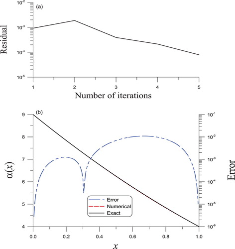
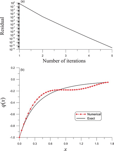
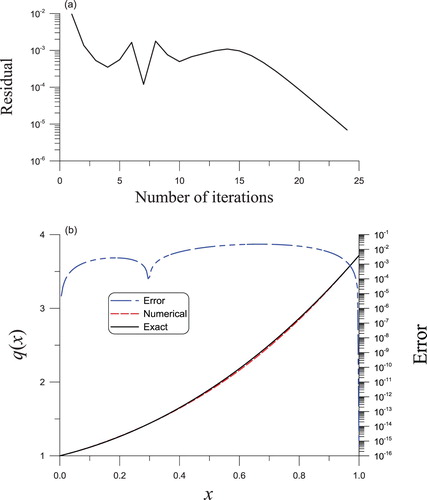
If m = 4, $\epsilon ={10}^{-4}$, the convergence of the iterative algorithm appears in five steps as plotted in Figure 1(a). Upon making a comparison between the reconstructed $\alpha (x)$ and the actual $\alpha (x)$, an ideal consequence with a maximum error of $1.1\times {10}^{-2}$ is derived presented by the dashed line in Figure 1(b). The errors are shown by a dashed-dotted line.

Figure 1. The solved linear Sturm–Liouville equation of second order in Example 3.1 through the BFM algorithm: (a) convergence rate, (b) a comparison of the reconstructed and actual leading coefficients, in which the red and black curves overlap.

Example 3.2

The example is given by (29) $q(x)=x^2,\alpha (x)=(x-3{)}^2+\sin (\pi x),w(x)={\mathrm{e}}^x,F(w)=w^2,$(29) in which the actual $H(x)$ can be obtained based on Equation (3(3) $-[\alpha (x)w^{\mathrm{\prime }}(x){]}^{\mathrm{\prime }}+q(x)F(w(x))=H(x),x\in (0,\ell ),$(3) ). The new method is used to reconstruct $\alpha (x)$.

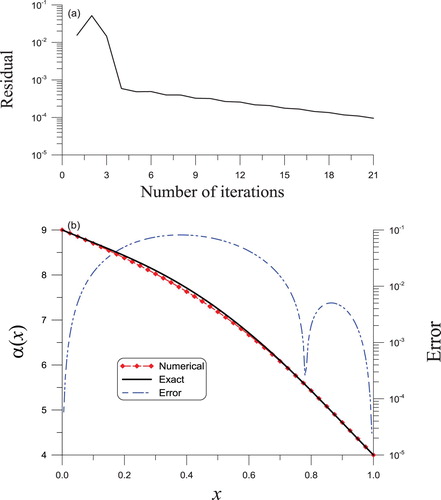
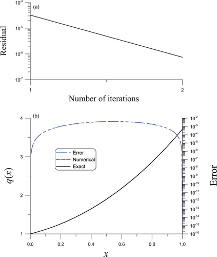
With m = 2 and $\epsilon ={10}^{-4}$, the iterative algorithm converges in 21 steps presented in Figure 2(a). Upon making a comparison between the reconstructed $\alpha (x)$ and the actual $\alpha (x)$, an acceptable result with a maximum error of $8.2\times {10}^{-2}$ is derived presented by dashed line filled with red diamonds in Figure 2(b). The errors are shown by dashed-dotted line.

Figure 2. The solved nonlinear Sturm–Liouville equation of second order in Example 3.2 through the BFM algorithm, (a) convergence rate, (b) a comparison of the reconstructed and actual leading coefficients.

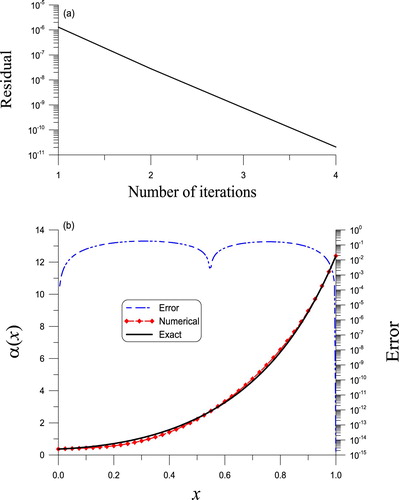
Example 3.3

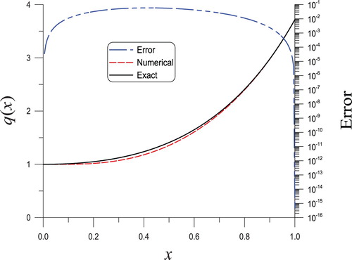
Consider (30) $\begin{array}{rl}q(x)& =x^2,\alpha (x)=3x^2+2x^3+\exp (x^2+2x-1),\\ w(x)& =x^4-2x^3+x^2,F(w)=w^2,\end{array}$(30) in which the actual $H(x)$ can be obtained based on Equation (3(3) $-[\alpha (x)w^{\mathrm{\prime }}(x){]}^{\mathrm{\prime }}+q(x)F(w(x))=H(x),x\in (0,\ell ),$(3) ). With m = 3 and $\epsilon ={10}^{-10}$, the iterative algorithm converges in four steps as presented in Figure 3(a). Upon making a comparison between the reconstructed $\alpha (x)$ and the actual $\alpha (x)$, an ideal consequence with a maximum error of 0.185 is derived presented by the dashed line filled with red diamonds in Figure 3(b).

Figure 3. The solved nonlinear Sturm–Liouville equation of second order in Example 3.3 through the BFM algorithm, (a) convergence rate, (b) a comparison of the reconstructed and actual leading coefficients.

4. Identifying $q(x)$ in the nonlinear Sturm–Liouville operator

To reconstruct $q(x)$ in Equation (3(3) $-[\alpha (x)w^{\mathrm{\prime }}(x){]}^{\mathrm{\prime }}+q(x)F(w(x))=H(x),x\in (0,\ell ),$(3) ), assume that it is possible to expand the uncertain potential function $q(x)$ by (31) $q(x)=e(x)+\sum _{k=1}^m{c}_k{E}_k(x),$(31) in which (32) $e(x)=\frac{1}{{\ell }^3}[2q_0-2q_{\ell }+q_0^{\mathrm{\prime }}\ell +q_{\ell }^{\mathrm{\prime }}\ell ]x^3-\frac{1}{{\ell }^2}[3q_0-3q_{\ell }+2q_0^{\mathrm{\prime }}\ell +q_{\ell }^{\mathrm{\prime }}\ell ]x^2+q_0^{\mathrm{\prime }}x+q_0,$(32) and $q(0)=q_0$, $q(\ell )=q_{\ell }$, $q^{\mathrm{\prime }}(0)=q_0^{\mathrm{\prime }}$ and $q^{\mathrm{\prime }}(\ell )=q_{\ell }^{\mathrm{\prime }}$ are given.

The numerical algorithm is close to that in Section 3, of which the linear system is modified as (33) $\begin{array}{rl}& \sum _{k=1}^m{c}_k{\int }_0^{\ell }Q(E_j(x)+b(x))E_k(x)\mathrm{d}x\\ & =d_0-{\int }_0^{\ell }\alpha (x)[E_j^{\mathrm{\prime }}(x)+b^{\mathrm{\prime }}(x){]}^2\mathrm{d}x\\ & +{\int }_0^{\ell }H(x)[E_j(x)+b(x)]\mathrm{d}x-{\int }_0^{\ell }e(x)Q(E_j(x)+b(x))\mathrm{d}x.\end{array}$(33) This linear system can be solved to determine the expansion coefficients $c_k,k=1,\dots ,m$, and afterwards $q(x)$ can be estimated by Equation (31(31) $q(x)=e(x)+\sum _{k=1}^m{c}_k{E}_k(x),$(31) ).

Consider the linear inverse Sturm–Liouville problem in Equations (1(1) $\begin{array}{rl}& -\frac{\mathrm{d}}{\mathrm{d}x}[p(x)\frac{\mathrm{d}w(x)}{\mathrm{d}x}]+q(x)w(x)=\lambda s(x)w(x),0<x<\ell ,\end{array}$(1) ) and (2(2) $\begin{array}{rl}& w(0)=0,w(\ell )=0.\end{array}$(2) ), ${\gamma }_j$ can be found by (34) ${\gamma }_j=\frac{-a_1-\sqrt{|a_1^2-4a_0{a}_2|}}{2a_2},$(34) in which (35) $\begin{array}{rl}& a_2:={\int }_0^{\ell }\{p(x)B_j^{\mathrm{\prime }}(x{)}^2+[q(x)-\lambda s(x)]B_j^2(x)\}\mathrm{d}x,\\ & a_1:={\int }_0^{\ell }\{2p(x)B_j^{\mathrm{\prime }}(x)[B_{j+1}^{\mathrm{\prime }}(x)+b^{\mathrm{\prime }}(x)]+2[q(x)-\lambda s(x)]B_j(x)[B_{j+1}(x)+b(x)]\}\mathrm{d}x,\\ & a_0:={\int }_0^{\ell }\{p(x)[B_{j+1}^{\mathrm{\prime }}(x)+b^{\mathrm{\prime }}(x){]}^2+[q(x)-\lambda s(x)][B_{j+1}(x)+b(x){]}^2\}\mathrm{d}x-d_0.\end{array}$(35) The expansion coefficients $c_k$ in Equation (31(31) $q(x)=e(x)+\sum _{k=1}^m{c}_k{E}_k(x),$(31) ) are determined according to the following linear system: (36) $\begin{array}{rl}& c_k{\int }_0^{\ell }[E_j(x)+b(x){]}^2{E}_k(x)\mathrm{d}x\\ & =d_0-{\int }_0^{\ell }p(x)[E_j^{\mathrm{\prime }}(x)+b^{\mathrm{\prime }}(x){]}^2\mathrm{d}x\\ & +{\int }_0^{\ell }\lambda s(x)[E_j(x)+b(x){]}^2\mathrm{d}x-{\int }_0^{\ell }e(x)[E_j(x)+b(x)]\mathrm{d}x.\end{array}$(36) If λ is provided, $q(x)$ can be reconstructed by the equations.

Example 4.1

The linear example is given by (37) $\begin{array}{rl}& q(x)=2x^2+x^3+{\mathrm{e}}^x,\alpha (x)=(x-3{)}^2,y(x)={\mathrm{e}}^x,F(w)=w,\\ & H(x)={\mathrm{e}}^x(x^3+x^2+4x-3)+{\mathrm{e}}^{2x},\end{array}$(37) in which the potential function $q(x)$ can be reconstructed.

With m = 2 and $\epsilon ={10}^{-5}$, the convergence of the iterative algorithm appears in two steps as presented in Figure 4(a). After making a comparison with the actual $q(x)$ in Figure 4(b), an excellent result is derived as shown by the dashed line. The maximum error is $4.62\times {10}^{-3}$.

Figure 4. The solved nonlinear Sturm–Liouville equation of second order in Example 4.1 through the BFM algorithm, (a) convergence rate, (b) a comparison of the reconstructed and actual potential functions, in which the red and black curves overlap.

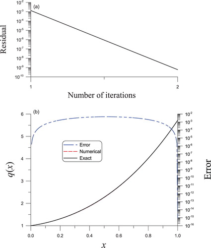
Example 4.2

Consider a linear inverse Sturm–Liouville problem as a second test example with (38) $\begin{array}{rl}& -[t^{-1}{w}^{\mathrm{\prime }}(t){]}^{\mathrm{\prime }}-t^{-3}w(t)=\lambda t^{-3}w(t),\\ & w(1)=w(e)=0.\end{array}$(38) The solution of the direct problem is as follows: eigenvalues are ${\lambda }_k=k^2{\pi }^2,k\in \mathbb{N}$, and eigenfunctions are $w_k=t\sin (k\pi \ln t)$. For the inverse problem, letting the eigenvalues ${\lambda }_k=k^2{\pi }^2$, we manage to find the potential function numerically.

Make a variable transformation from t to x = t−1: (39) $\begin{array}{rl}& -[(x+1{)}^{-1}{w}^{\mathrm{\prime }}(x){]}^{\mathrm{\prime }}-(x+1{)}^{-3}w(x)=\lambda (x+1{)}^{-3}w(x),\\ & w(0)=w(e-1)=0.\end{array}$(39) Then, make the second eigenvalue the input, and utilize Equations (34(34) ${\gamma }_j=\frac{-a_1-\sqrt{|a_1^2-4a_0{a}_2|}}{2a_2},$(34) )–(36(36) $\begin{array}{rl}& c_k{\int }_0^{\ell }[E_j(x)+b(x){]}^2{E}_k(x)\mathrm{d}x\\ & =d_0-{\int }_0^{\ell }p(x)[E_j^{\mathrm{\prime }}(x)+b^{\mathrm{\prime }}(x){]}^2\mathrm{d}x\\ & +{\int }_0^{\ell }\lambda s(x)[E_j(x)+b(x){]}^2\mathrm{d}x-{\int }_0^{\ell }e(x)[E_j(x)+b(x)]\mathrm{d}x.\end{array}$(36) ) to reconstruct the uncertain potential function $q(x)$. With m = 2 and $\epsilon ={10}^{-10}$, the convergence of the iterative algorithm appears in five steps presented in Figure 5(a). By making a comparison with the actual $q(x)=-(x+1{)}^{-3}$ in Figure 5(b), a decent consequence is derived depicted by the dashed line, in which the maximum error is $7.233\times {10}^{-2}$.

Figure 5. The solved nonlinear Sturm–Liouville equation of second order in Example 4.2 through the BFM algorithm, (a) convergence rate, (b) a comparison of the reconstructed and actual potential functions.

Example 4.3

This example is a nonlinear inverse Sturm–Liouville problem, given by (40) $q(x)=x^2+{\mathrm{e}}^x,\alpha (x)=(x-3{)}^2+\sin (\pi x),w(x)={\mathrm{e}}^x,F(w)=w^2,$(40) in which the actual $H(x)$ can be obtained based on Equation (3(3) $-[\alpha (x)w^{\mathrm{\prime }}(x){]}^{\mathrm{\prime }}+q(x)F(w(x))=H(x),x\in (0,\ell ),$(3) ), and $q(x)$ can be reconstructed by the BFM.

Under m = 2 and $\epsilon ={10}^{-5}$, the convergence of the iterative algorithm appears in two steps as shown in Figure 6(a). Upon making a comparison between the rebuilt $q(x)$ with the actual $q(x)$, an ideal result is derived with a maximum error of $3.94\times {10}^{-3}$ presented by the dashed line in Figure 6(b).

Figure 6. The solved nonlinear Sturm–Liouville equation of second order in Example 4.3 through the BFM algorithm, (a) convergence rate, (b) a comparison of the reconstructed potential functions, in which the red and black curves overlap.

Example 4.4

Given by (41) $q(x)=x^3+{\mathrm{e}}^{x^2},\alpha (x)=(x-3{)}^2,w(x)=x^2,F(w)=\sin w,$(41) in which the actual $H(x)$ can be obtained based on Equation (3(3) $-[\alpha (x)w^{\mathrm{\prime }}(x){]}^{\mathrm{\prime }}+q(x)F(w(x))=H(x),x\in (0,\ell ),$(3) ).

Under m = 3 and $\epsilon ={10}^{-4}$, the convergence of the iterative algorithm appears in one step. Upon comparison with the actual $q(x)$, an ideal result is derived with a maximum error of $5.86\times {10}^{-2}$ as shown by the dashed line in Figure 7.

Figure 7. The solved nonlinear Sturm–Liouville equation of second order in Example 4.4 through the BFM algorithm, (a) convergence rate, (b) a comparison of the reconstructed and actual potential functions.

5. Nonlinear convection inverse Sturm–Liouville problems

In this section the results are extended to the nonlinear convection inverse Sturm–Liouville problem in Equation (4(4) $-[\alpha (x)w^{\mathrm{\prime }}(x){]}^{\mathrm{\prime }}+q(x)F(w(x))+G(w(x))w^{\mathrm{\prime }}(x)=H(x),x\in (0,\ell ),$(4) ). First, multiplying Equation (4(4) $-[\alpha (x)w^{\mathrm{\prime }}(x){]}^{\mathrm{\prime }}+q(x)F(w(x))+G(w(x))w^{\mathrm{\prime }}(x)=H(x),x\in (0,\ell ),$(4) ) by $w(x)$; second, integrating it from x = 0 to $x=\ell$; finally, utilizing integration partially and using Equations (5(5) $\begin{array}{rl}& w(0)=w_0,w(\ell )=w_{\ell },w^{\mathrm{\prime }}(0)=w_0^{\mathrm{\prime }},w^{\mathrm{\prime }}(\ell )=w_{\ell }^{\mathrm{\prime }},\end{array}$(5) ) and (6(6) $\begin{array}{rl}& \alpha (0)={\alpha }_0,\alpha (\ell )={\alpha }_{\ell },{\alpha }^{\mathrm{\prime }}(0)={\alpha }_0^{\mathrm{\prime }},{\alpha }^{\mathrm{\prime }}(\ell )={\alpha }_{\ell }^{\mathrm{\prime }}.\end{array}$(6) ), the energy identity is obtained: (42) $\begin{array}{rl}& {\int }_0^{\ell }\{\alpha (x)w^{\mathrm{\prime }}(x{)}^2+q(x)Q(w(x))-H(x)w(x)\}\mathrm{d}x\\ & ={\alpha }_{\ell }{w}_{\ell }{w}_{\ell }^{\mathrm{\prime }}-{\alpha }_0{w}_0{w}_0^{\mathrm{\prime }}+P(w_0)-P(w_{\ell })=:D_0=d_0+P(w_0)-P(w_{\ell }),\end{array}$(42) in which (43) $P(w):=\int wG(w)\mathrm{d}w.$(43) Now not only the deformation energy but also the potential energy and dissipation energy and even external work are brought into balance. Then inserting $w(x)=y(x)+b(x)$, we obtain (44) ${\int }_0^{\ell }\{\alpha (x)[y^{\mathrm{\prime }}(x)+b^{\mathrm{\prime }}(x){]}^2+q(x)Q(y(x)+b(x))-H(x)[y(x)+b(x)]\}\mathrm{d}x=D_0,$(44) which has similarities to Equation (11(11) $\begin{array}{rl}& {\int }_0^{\ell }\{\alpha (x)[y^{\mathrm{\prime }}(x)+b^{\mathrm{\prime }}(x){]}^2+q(x)Q(y(x)+b(x))-H(x)[y(x)+b(x)]\}\mathrm{d}x\\ & ={\alpha }_{\ell }{w}_{\ell }{w}_{\ell }^{\mathrm{\prime }}-{\alpha }_0{w}_0{w}_0^{\mathrm{\prime }}=:d_0,\end{array}$(11) ) with $d_0$ substituted by $D_0$.

The numerical algorithms acquired in Section 3 to decide $\alpha (x)$ and that obtained in Section 4 to identify $q(x)$ are also applicable to the nonlinear convection inverse Sturm–Liouville problem (4(4) $-[\alpha (x)w^{\mathrm{\prime }}(x){]}^{\mathrm{\prime }}+q(x)F(w(x))+G(w(x))w^{\mathrm{\prime }}(x)=H(x),x\in (0,\ell ),$(4) ), in which $d_0$ has to be substituted by $D_0$. The source term $H(x)$ should be computed from Equation (4(4) $-[\alpha (x)w^{\mathrm{\prime }}(x){]}^{\mathrm{\prime }}+q(x)F(w(x))+G(w(x))w^{\mathrm{\prime }}(x)=H(x),x\in (0,\ell ),$(4) ).

Example 5.1

Given by (45) $q(x)=x^2,\alpha (x)=(x-3{)}^2+\sin (\pi x),w(x)={\mathrm{e}}^x,F(w)=w^2,G(w)=w^3,$(45) in which the actual $H(x)$ can be obtained based on Equation (4(4) $-[\alpha (x)w^{\mathrm{\prime }}(x){]}^{\mathrm{\prime }}+q(x)F(w(x))+G(w(x))w^{\mathrm{\prime }}(x)=H(x),x\in (0,\ell ),$(4) ) and $\alpha (x)$ can be rebuilt by the new method.

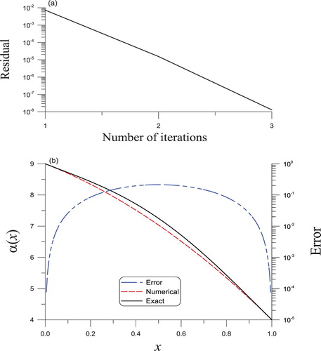
Under m = 3 and $\epsilon ={10}^{-4}$, the convergence of the iterative algorithm appears in three steps as shown in Figure 8(a). Upon making a comparison between the reconstructed $\alpha (x)$ with the actual $\alpha (x)$, an ideal result is derived with a maximum error of 0.21 depicted by the dashed line filled by red diamonds in Figure 8(b). The errors are shown by the dashed-dotted line.

Figure 8. The solved nonlinear Sturm–Liouville equation having a nonlinear convective term of second order in Example 5.1 through the BFM algorithm, (a) convergence rate, (b) a comparison of the reconstructed and actual leading coefficients.

Example 5.2

This example is given by (46) $\begin{array}{rl}q(x)& =x^2+{\mathrm{e}}^x,\alpha (x)=(x-3{)}^2+\sin (\pi x),\\ w(x)& ={\mathrm{e}}^x,F(w)=w^2,G(w)=w^2,\end{array}$(46) in which the actual $H(x)$ can be obtained based on Equation (4(4) $-[\alpha (x)w^{\mathrm{\prime }}(x){]}^{\mathrm{\prime }}+q(x)F(w(x))+G(w(x))w^{\mathrm{\prime }}(x)=H(x),x\in (0,\ell ),$(4) ).

Under m = 2 and $\epsilon ={10}^{-4}$, the convergence of the iterative algorithm appears in 24 steps as shown in Figure 9(a). Upon making a comparison between the reconstructed $q(x)$ with the actual $q(x)$, an acceptable result is derived with a maximum error of $2.25\times {10}^{-2}$ shown by the dashed line in Figure 9(b).

Figure 9. The solved nonlinear Sturm–Liouville equation having a nonlinear convective term of second order in Example 5.2 through the BFM algorithm, (a) convergence rate, (b) a comparison of the reconstructed and actual potential functions, where the red and black curves overlap.

6. Conclusions

In the present research, the reconstruction problems including a second-order nonlinear Sturm–Liouville operator with a nonlinear convective term have been settled through the linear systems used in deciding the expansion coefficients of the uncertain leading coefficient and potential function. The energy identity obtained from the governing equation has been adopted in constructing a linear space of the energetic boundary functions, which both qualify the over-specified boundary conditions and maintain the energy. Therefore, the uncertain potential functions and leading coefficients in the linear space can be reconstructed rapidly with the assistance of the boundary data. Numerical instances suggest that the introduced energetic BFM, for the recovery of nonlinear Sturm-Liouville operators containing a nonlinear convective term, is exceedingly effective and accurate.

Disclosure statement

No potential conflict of interest was reported by the authors.

Additional information

Funding

The Fundamental Research Funds for the Central Universities under the Grant Number 2017B05714 for the financial support to the first author Chein-Shan Liu are highly appreciated. Botong Li acknowledges support from the Fundamental Research Funds for the Central Universities.

References

- Gelfand IM, Levitan BM. On the determination of a differential equation from its spectral function. Amer Math Soc Transl. 1951;1:253–304.
- McLaughlin JR. Analytical methods for recovering coefficients in differential equations from spectral data. SIAM Rev. 1986;28:53–72. doi: 10.1137/1028003
- Bondarenko NP, Buterin SA, Vasiliev SV. An inverse spectral problem for Sturm–Liouville operators with frozen argument. J Math Anal Appl. 2019;472:1028–1041. doi: 10.1016/j.jmaa.2018.11.062
- Sat M, Panakhov ES. A uniqueness theorem for Bessel operator from interior spectral data. Abstr Appl Anal. 2013; ID 713654.
- Chu MT. Inverse eigenvalue problems. SIAM Rev. 1998;40:1–39. doi: 10.1137/S0036144596303984
- Andrew AL. Numerical solution of inverse Sturm–Liouville problems. ANZIAM J. 2004;45E:C326–C337. doi: 10.21914/anziamj.v45i0.891
- Paine J. A numerical method for the inverse Sturm–Liouville problem. SIAM Sci Stat Comput. 1984;5:149–156. doi: 10.1137/0905011
- McLaughlin JR. Inverse spectral theory using nodal points as data–a uniqueness result. J Differ Equ. 1988;73:354–362. doi: 10.1016/0022-0396(88)90111-8
- Browne PJ, Sleeman BD. Inverse nodal problem for Sturm-Liouville equation with eigenparameter depend boundary conditions. Inverse Probl. 1996;12:377–381. doi: 10.1088/0266-5611/12/4/002
- Cheng YH, Law CK, Tsay J. Remarks on a new inverse nodal problem. J Math Anal Appl. 2000;248:145–155. doi: 10.1006/jmaa.2000.6878
- Hald O, McLaughlin JR. Solutions of inverse nodal problems. Inverse Probl. 1989;5:307–347. doi: 10.1088/0266-5611/5/3/008
- Yang FX. A solution of the inverse nodal problem. Inverse Probl. 1997;13:203–213. doi: 10.1088/0266-5611/13/1/016
- Sat M, Shieh CT. Inverse nodal problems for integro-differential operators with a constant delay. J Inverse Ill-posed Probl. 2019;27:501–509. doi: 10.1515/jiip-2018-0088
- Boley D, Golub GH. A survey of matrix inverse eigenvalue problems. Inverse Probl. 1987;3:595–622. doi: 10.1088/0266-5611/3/4/010
- Liu CS. Solving an inverse Sturm–Liouville problem by a Lie-group method. Boundary Value Problems. 2008; Article ID 749865.
- Liu CS, Atluri SN. A novel fictitious time integration method for solving the discretized inverse Sturm–Liouville problems, for specified eigenvalues. Comput Model Eng Sci. 2008;36:261–285.
- Hasanov A, Shores TS. Solution of an inverse coefficient problem for an ordinary differential equation. Appl Anal. 1997;67:11–20. doi: 10.1080/00036819708840594
- Kaltenbacher B. A projection-regularized Newton method for nonlinear ill-posed problems and its application to parameter identification problems with finite element discretization. SIAM J Numer Anal. 2000;37:1885–1908. doi: 10.1137/S0036142998347322
- Hasanov A, Pektas B. Simulation of ill-conditioned situations in inverse coefficient problem for the Sturm–Liouville operator based on boundary measurements. Math Comput Simul. 2002;61:47–52. doi: 10.1016/S0378-4754(02)00134-9
- Hasanov A. An inverse polynomial method for the identification of the leading coefficient in the Sturm–Liouville operator from boundary measurements. Appl Math Comput. 2003;140:501–515.
- Liu CS. An inverse problem for computing a leading coefficient in the Sturm–Liouville operator by using the boundary data. Appl Math Comput. 2011;218:4245–4259.
- Liu CS. Identifying a rigidity function distributed in static composite beam by the boundary functional method. Compos Struct. 2017;176:996–1004. doi: 10.1016/j.compstruct.2017.06.003
- Liu CS, Li B. Reconstructing a second-order Sturm–Liouville operator by an energetic boundary function iterative method. Appl Math Lett. 2017;73:49–55. doi: 10.1016/j.aml.2017.04.023