A generalized Newton iteration for computing the solution of the inverse Henderson problem

ABSTRACT

We develop a generalized Newton scheme called IHNC (inverse hypernetted-chain iteration) for the construction of effective pair potentials for systems of interacting point-like particles. The construction is realized in such a way that the distribution of the particles matches a given radial distribution function. The IHNC iteration uses the hypernetted-chain integral equation for an approximate evaluation of the inverse of the Jacobian of the forward operator.

In contrast to the full Newton method realized in the Inverse Monte Carlo (IMC) scheme, the IHNC algorithm requires only a single molecular dynamics computation of the radial distribution function per iteration step and no further expensive cross-correlations. Numerical experiments are shown to demonstrate that the method is as efficient as the IMC scheme, and that it easily allows to incorporate thermodynamical constraints.

Keywords:

• Coarse-graining
• radial distribution function
• effective potential
• Iterative Boltzmann Inversion
• Inverse Monte Carlo

AMS subject classifications:

• 65Z05
• 82B21

1. Introduction

A common problem in material science is the quantification of interactions between a set of given particles. For example, in computer simulations of complex materials, where all sorts of numerical multiscale techniques are inevitable tools to treat relevant timescales and/or spatial resolutions (cf., e.g. Potestio, Peter, and Kremer [1]), larger atomistic structures are often replaced by artificial particles, so-called beads, and the simulation of these beads requires the knowledge of effective interactions between them and other molecules or atoms.

In the simplest case, one may assume that the beads are point-like particles, whose interactions are governed by a potential $u=u(r)$, which only depends on the distance r>0 of each interacting pair of particles and vanishes in the limit $r\to \mathrm{\infty }$. According to Henderson [2] such a pair potential $u=u(r)$ is uniquely determined by the so-called radial distribution function $g=g(r)$, which measures the number of particle pairs with a given distance in a homogeneous fluid in thermal equilibrium. The inverse Henderson problem of computing the pair potential from the given radial distribution is therefore exactly what needs to be solved in order to settle the aforementioned problem in physical chemistry.

One of the difficulties with this problem is the fact that the associated map (1) $G:u\mapsto g,$(1) which takes the pair potential onto the corresponding radial distribution function (for specified values of density and temperature of the fluid) is not given in closed terms, but has to be evaluated numerically, using expensive molecular dynamics or Monte-Carlo simulations. It goes without saying that the inverse map $G^{-1}$ is not known, either. Methods for solving the inverse Henderson problem therefore can be distinguished in two classes: one class uses closed-form approximations of G or $G^{-1}$, respectively, most notably the hypernetted-chain or the Percus–Yevick approximations, cf., e.g. Ben–Naim [3] or Hansen and McDonald [4]; the other class uses iterative schemes which start from a certain educated guess $u_k$ of u, simulate the corresponding radial distribution function $g_k=G(u_k)$ and use this information to determine an improved approximation $u_{k+1}$ by some sophisticated update rule, proceeding in this manner until convergence. Most prominent representatives of the latter class are the Iterative Boltzmann Inversion (IBI) or Inverse Monte Carlo (IMC); cf., e.g. Mirzoev and Lyubartsev [5], Rühle et al. [6] or Tóth [7].

In this paper, we suggest a new method of the second class, i.e. an iterative method, which combines the advantages of the two aforementioned schemes, namely the simplicity and robustness of IBI, and the rapid convergence of IMC for an appropriate initial guess. Our method is a generalized Newton iteration – as opposed to IMC, which corresponds to the much more expensive full Newton scheme for inverting (1(1) $G:u\mapsto g,$(1) ) – and we use the hypernetted-chain approximation to compute a simplified derivative of G. We show by numerical examples for simulated and measured radial distribution data that the method outperforms IBI and requires about the same number of iterations as does IMC, even when the density and the temperature of the fluid are near a phase transition. We also demonstrate how to include thermodynamical constraints like a known value for the pressure of the system into our scheme. In this work, we only treat the case of a homogeneous fluid of single particles; we plan to show in a forthcoming paper how to extend the method to binary mixtures.

The outline of this paper is as follows. In the following section, we briefly summarize the necessary ingredients from statistical mechanics which are fundamental for this work. Then, in Section 3, we derive the approximation of the inverse of the Jacobian of G which will be used for our generalized Newton scheme. Section 4 presents the mathematical core of this paper and is concerned with the well-posedness of different variants of our algorithm. Readers who are only interested in the algorithms and in implementation details can skip this part without any loss. In the subsequent two sections, we then discuss the numerical implementation and further extensions of these schemes; in particular, we show in Section 6 how to incorporate pressure constraints. Finally, numerical results for some benchmark systems are presented in Section 7. In the appendix, we include a proof for an extension of the classical Wiener lemma (cf., e.g. Jörgens [8]) to some weighted $L^{\mathrm{\infty }}$ space, which is needed for our mathematical analysis.

2. Mathematical setting of the problem

Consider an ensemble of identical classical point-like particles in thermodynamical equilibrium, where the interaction of the particles is given in terms of a pair potential $u:{\mathbb{R}}^{+}\to \mathbb{R}$ of Lennard–Jones type, i.e. there exist a core radius $r_0>0$ and a parameter $\alpha >3$ such that (2) $\begin{array}{rl}u(r)\phantom{|}& \ge a{r}^{-\alpha },r\le r_0,\\ |u(r)|& \le b{r}^{-\alpha },r\ge r_0,\end{array}$(2) for suitable constants a, b>0. We assume that the number of particles and the size of the spatial domain under consideration are so big that one can treat this ensemble in the thermodynamical limit, i.e. as if it fills the full space ${\mathbb{R}}^3$. For our mathematical analysis, we further assume that the counting density ${\rho }_0>0$ of the ensemble is sufficiently small and the temperature T>0 is sufficiently large, so that the system is in its so-called gas phase, cf., e.g. Ruelle [9, p. 84].

The radial distribution function $g:{\mathbb{R}}^{+}\to {\mathbb{R}}^{+}$, referred to in the introduction, measures the number of particle pairs at distance r>0, normalized in such a way that $g(r)\to 1$ as $r\to \mathrm{\infty }$; see [4] for the precise definition of this function. Then, as shown in [10], the map G of (1(1) $G:u\mapsto g,$(1) ), which takes u onto g, is well-defined and differentiable in a certain neighbourhood of u with respect to the Banach space $\mathcal{V}$ of perturbations v of u, for which the corresponding norm (3) $\Vert v{\Vert }_{\mathcal{V}}=max\{\Vert v/u{\Vert }_{(0,r_0]},\Vert \varrho v{\Vert }_{[r_0,\mathrm{\infty })}\}$(3) is sufficiently small; here, (4) $\varrho (r)=(1+r^2{)}^{\alpha /2},r\ge 0,$(4) is a weight function associated with the parameter α of (2(2) $\begin{array}{rl}u(r)\phantom{|}& \ge a{r}^{-\alpha },r\le r_0,\\ |u(r)|& \le b{r}^{-\alpha },r\ge r_0,\end{array}$(2) ), and for a real interval $\mathcal{I}\subset \mathbb{R}$ the expression $\Vert \cdot {\Vert }_{\mathcal{I}}$ refers to the supremum norm of real functions defined on this respective interval.

In [11], it has been shown that the so-called pair correlation function h = g−1 for a Lennard–Jones type pair potential given by (2(2) $\begin{array}{rl}u(r)\phantom{|}& \ge a{r}^{-\alpha },r\le r_0,\\ |u(r)|& \le b{r}^{-\alpha },r\ge r_0,\end{array}$(2) ) belongs to the Banach space $L_{\varrho }^{\mathrm{\infty }}$ of functions $f\in L^{\mathrm{\infty }}$ with finite norm (5) $\Vert f{\Vert }_{L_{\varrho }^{\mathrm{\infty }}}=\Vert \varrho f{\Vert }_{(0,\mathrm{\infty })},$(5) where ϱ is defined in (4(4) $\varrho (r)=(1+r^2{)}^{\alpha /2},r\ge 0,$(4) ). Since $\alpha >3$, the radially symmetric extension of any $f\in L_{\varrho }^{\mathrm{\infty }}$ to the full space ${\mathbb{R}}^3$ is absolutely integrable and has a well-defined (three-dimensional) continuous Fourier transform. This is important, because although u, g, and h are defined as functions of a positive argument r>0, they can be viewed as representations of radial functions of a three-dimensional spatial variable in full space. In particular, the Fourier transform of the corresponding extension of h – which is again radially symmetric and can therefore be represented by a function $\hat{h}:[0,\mathrm{\infty })\to \mathbb{R}$ by some slight abuse of the standard notation – is used to define the structure factor (6) $S(\omega )=1+{\rho }_0\hat{h}(\omega ),\omega \ge 0,$(6) which is known to be continuous and nonnegative.

Going one step further, if $f_1,f_2\in L_{\varrho }^{\mathrm{\infty }}$, then the three-dimensional convolution integral of their radially symmetric extensions to ${\mathbb{R}}^3$ is again a radial function and – as has also been shown in [11] – its representation (as a function defined in ${\mathbb{R}}^{+}$) again belongs to $L_{\varrho }^{\mathrm{\infty }}$; we adopt the notation $f_1\ast f_2$ for the resulting convolution product, which turns $L_{\varrho }^{\mathrm{\infty }}$ into a (commutative) Banach algebra.

Proposition 2.1

Let u be a Lennard–Jones type pair potential (2(2) $\begin{array}{rl}u(r)\phantom{|}& \ge a{r}^{-\alpha },r\le r_0,\\ |u(r)|& \le b{r}^{-\alpha },r\ge r_0,\end{array}$(2) ) with parameter $\alpha >3$, and let the counting density ${\rho }_0$ of the ensemble be sufficiently small. Using the pair correlation function h of this ensemble and the above definition of the convolution product in $L_{\varrho }^{\mathrm{\infty }}$, define (7) $A:L_{\varrho }^{\mathrm{\infty }}\to L_{\varrho }^{\mathrm{\infty }},A:f\mapsto {\rho }_{0}h\ast f.$(7) Then I + A is invertible in $\mathcal{L}(L_{\varrho }^{\mathrm{\infty }})$, if the structure factor (6(6) $S(\omega )=1+{\rho }_0\hat{h}(\omega ),\omega \ge 0,$(6) ) is strictly positive.

The proof of this result follows from a weighted version of the Wiener lemma, stated and proved in the appendix, cf. Lemma A.1.

Under the assumptions of Proposition 2.1, it follows in particular that the so-called Ornstein–Zernike relation (8) $c+{\rho }_{0}h\ast c=h$(8) has a unique solution $c\in L_{\varrho }^{\mathrm{\infty }}$, known as the direct correlation function, cf. [4]. Then, with $k_{\mathrm{B}}$ the Boltzmann constant and $\beta =\frac{1}{k_{\mathrm{B}}T}$ the inverse temperature, the hypernetted-chain approximation mentioned in the introduction states that (9) $g\approx e^{-\beta u+h-c}.$(9) Historically (9(9) $g\approx e^{-\beta u+h-c}.$(9) ) has been used to approximate g without lengthy molecular dynamics simulations, but by solving a (nonlinear) integral equation instead. On the other hand, (9(9) $g\approx e^{-\beta u+h-c}.$(9) ) can be solved for u to provide an explicit approximation $u_{\mathrm{HNC}}$ of the true pair potential, namely (10) $u_{\mathrm{HNC}}=U(g)=-\frac{1}{\beta }\log g+\frac{1}{\beta }(h-c),$(10) which only depends on quantities that are readily available from the given radial distribution function.

We close this section by formally differentiating U of (10(10) $u_{\mathrm{HNC}}=U(g)=-\frac{1}{\beta }\log g+\frac{1}{\beta }(h-c),$(10) ) to determine the impact of small perturbations $g^{\prime }$ of g on $u_{\mathrm{HNC}}$, namely (11) $U^{\prime }(g)g^{\prime }=-\frac{1}{\beta }\frac{g^{\prime }}{g}+\frac{1}{\beta }(g^{\prime }-c^{\prime }),$(11) where $c^{\prime }$ is the derivative of c with respect to g or h, respectively: Using (8(8) $c+{\rho }_{0}h\ast c=h$(8) ) and the fact that $(L_{\varrho }^{\mathrm{\infty }},\ast )$ is a Banach algebra, we conclude that (12) $c^{\prime }+{\rho }_{0}h\ast c^{\prime }+{\rho }_0{g}^{\prime }\ast c=g^{\prime }.$(12) Convolving this equation with ${\rho }_{0}h$, adding the result to (12(12) $c^{\prime }+{\rho }_{0}h\ast c^{\prime }+{\rho }_0{g}^{\prime }\ast c=g^{\prime }.$(12) ) again, and using the associativity and commutativity of the convolution product, we obtain $c^{\prime }+2{\rho }_{0}h\ast c^{\prime }+{\rho }_0^{2}h\ast h\ast c^{\prime }+{\rho }_0(c+{\rho }_{0}h\ast c)\ast g^{\prime }=g^{\prime }+{\rho }_{0}h\ast g^{\prime },$ and inserting (8(8) $c+{\rho }_{0}h\ast c=h$(8) ), this yields $c^{\prime }+2{\rho }_{0}h\ast c^{\prime }+{\rho }_0^{2}h\ast h\ast c^{\prime }=g^{\prime }.$ With the operator A of Proposition 2.1, the latter can be rewritten as $(I+A{)}^2{c}^{\prime }=g^{\prime },$ showing that $c^{\prime }\in L_{\varrho }^{\mathrm{\infty }}$ is well-defined when the structure factor is positive. Inserting this identity into (11(11) $U^{\prime }(g)g^{\prime }=-\frac{1}{\beta }\frac{g^{\prime }}{g}+\frac{1}{\beta }(g^{\prime }-c^{\prime }),$(11) ), we eventually obtain (13) $U^{\prime }(g)g^{\prime }=-\frac{1}{\beta }\frac{g^{\prime }}{g}+\frac{1}{\beta }\phi ,$(13) where (14) $\phi =(I+A{)}^{-2}(2I+A)A{g}^{\prime }.$(14)

3. Generalized Newton schemes for the inverse Henderson problem

We now present iterative algorithms for an approximate solution of the inverse Henderson problem, i.e. for determining a pair potential $\tilde{u}$, for which the associated radial distribution function $G(\tilde{u})$ is close to the given data g for specified values of ${\rho }_0$ and β.

One of the most successful methods of this kind is the Iterative Boltzmann Inversion (IBI) (15) $u_{k+1}=u_k+\frac{1}{\beta }\log \frac{g_k}{g},g_k=G(u_k),$(15) $k=0,1,2,\dots$, originally suggested by Schommers [12]. In (15(15) $u_{k+1}=u_k+\frac{1}{\beta }\log \frac{g_k}{g},g_k=G(u_k),$(15) ), as in Section 2, $g,g_k,u$ and $u_k$ are functions of $r\in (0,\mathrm{\infty })$, and we continue to omit the independent variable r as long as there is no danger of confusion. Note that each iteration of IBI requires an expensive evaluation of the forward operator G. IBI is widely used, because it has been found to be fairly robust. Soper, who redeveloped this scheme in [13], gave some heuristic arguments to support this observation. However, a rigorous convergence analysis is still lacking; see [11] for some preliminary results in this direction.

A certain shortcoming of IBI is that it may require quite a few iterations to determine a sufficiently accurate potential. In [14], Lyubartsev and Laaksonen therefore proposed the Newton method (16) $u_{k+1}=u_k+G^{\prime }(u_k{)}^{-1}(g-g_k),g_k=G(u_k),$(16) $k=0,1,2,\dots$, as an alternative. In this scheme, now called Inverse Monte Carlo (IMC),¹ the numerical evaluation of the Fréchet derivative of G can be implemented by using higher order statistics of the ensemble corresponding to some integrated 3- and 4-particle distribution functions. As it requires longer forward simulations to achieve sufficiently accurate statistics of these higher order distribution functions, each IMC iteration is much more expensive than one step of IBI. Another shortcoming of IMC is the need to start the iteration with a fairly accurate initial guess. It is therefore sometimes recommended to first run a number of IBI steps before switching to IMC, cf., e.g. Mirzoev and Lyubartsev [5] or Murtola et al. [15].

Here we consider a generalized Newton scheme, where $G^{\prime }(u_k{)}^{-1}$ in (16(16) $u_{k+1}=u_k+G^{\prime }(u_k{)}^{-1}(g-g_k),g_k=G(u_k),$(16) ) is replaced by some approximation. Note, for example, that the low-density approximation $G(u)\approx G_{\mathrm{LDL}}(u)=e^{-\beta u},$ which is correct of order $O({\rho }_0)$ as ${\rho }_0\to 0$, suggests to replace $G^{\prime }(u_k{)}^{-1}{g}^{\prime }\approx {G_{\mathrm{LDL}}^{\prime }(u)}^{-1}{g}^{\prime }=-\frac{1}{\beta }{e}^{\beta u}{g}^{\prime }\approx -\frac{1}{\beta }\frac{g^{\prime }}{g},$ cf. [16]. When using this approximation in (16(16) $u_{k+1}=u_k+G^{\prime }(u_k{)}^{-1}(g-g_k),g_k=G(u_k),$(16) ) we arrive at the iterative scheme (17) $u_{k+1}=u_k+\frac{1}{\beta }\frac{g_k-g}{g},k=0,1,2,\dots .$(17) Note that this is reminiscent of the IBI scheme (15(15) $u_{k+1}=u_k+\frac{1}{\beta }\log \frac{g_k}{g},g_k=G(u_k),$(15) ), because $\log \frac{g_k}{g}=\log (1+\frac{g_k-g}{g})\approx \frac{g_k-g}{g}$ for $g_k$ close to g. In fact, in numerical experiments that we have made, we did not observe a significant difference between the performance of the two iterative schemes (15(15) $u_{k+1}=u_k+\frac{1}{\beta }\log \frac{g_k}{g},g_k=G(u_k),$(15) ) and (17(17) $u_{k+1}=u_k+\frac{1}{\beta }\frac{g_k-g}{g},k=0,1,2,\dots .$(17) ).

We therefore propose a more sophisticated approximation of G, namely one that is based on the hypernetted-chain approximation (9(9) $g\approx e^{-\beta u+h-c}.$(9) ), which is correct of order $O({\rho }_0^2)$ as ${\rho }_0\to 0$, cf. [4], to obtain a useful compromise between IBI and IMC. To be specific, with U of (10(10) $u_{\mathrm{HNC}}=U(g)=-\frac{1}{\beta }\log g+\frac{1}{\beta }(h-c),$(10) ) we approximate (18) $G^{\prime }(u_k{)}^{-1}{g}^{\prime }\approx U^{\prime }(g)g^{\prime }=-\frac{1}{\beta }\frac{g^{\prime }}{g}+\frac{1}{\beta }\phi ,$(18) cf. (13(13) $U^{\prime }(g)g^{\prime }=-\frac{1}{\beta }\frac{g^{\prime }}{g}+\frac{1}{\beta }\phi ,$(13) ), where g is the measured radial distribution function and ϕ is given by (14(14) $\phi =(I+A{)}^{-2}(2I+A)A{g}^{\prime }.$(14) ) with A of (7(7) $A:L_{\varrho }^{\mathrm{\infty }}\to L_{\varrho }^{\mathrm{\infty }},A:f\mapsto {\rho }_{0}h\ast f.$(7) ). Inserting (18(18) $G^{\prime }(u_k{)}^{-1}{g}^{\prime }\approx U^{\prime }(g)g^{\prime }=-\frac{1}{\beta }\frac{g^{\prime }}{g}+\frac{1}{\beta }\phi ,$(18) ) into (16(16) $u_{k+1}=u_k+G^{\prime }(u_k{)}^{-1}(g-g_k),g_k=G(u_k),$(16) ) we thus obtain the iteration (19a) $u_{k+1}=u_k+\frac{1}{\beta }\frac{g_k-g}{g}+\frac{1}{\beta }{\phi }_k,k=0,1,2,\dots ,$(19a) with (19b) ${\phi }_k=(I+A{)}^{-2}(2I+A)A(g-g_k).$(19b) We call (19(19a) $u_{k+1}=u_k+\frac{1}{\beta }\frac{g_k-g}{g}+\frac{1}{\beta }{\phi }_k,k=0,1,2,\dots ,$(19a) ) the hypernetted-chain Newton iteration (HNCN). Take note that this approach does not involve a computation of the hypernetted-chain approximation $u_{\mathrm{HNC}}$ of (10(10) $u_{\mathrm{HNC}}=U(g)=-\frac{1}{\beta }\log g+\frac{1}{\beta }(h-c),$(10) ) itself; the hypernetted-chain approximation is only used formally to determine an approximate Newton inverse. Accordingly, when the iteration (19(19a) $u_{k+1}=u_k+\frac{1}{\beta }\frac{g_k-g}{g}+\frac{1}{\beta }{\phi }_k,k=0,1,2,\dots ,$(19a) ) converges, i.e. when $u_k\to u$ and $g_k\to g$ as $k\to \mathrm{\infty }$, then the limit u is the true solution of the Henderson problem for the given data.

Note that HNCN coincides with (17(17) $u_{k+1}=u_k+\frac{1}{\beta }\frac{g_k-g}{g},k=0,1,2,\dots .$(17) ) up to an additive correction term. The similarity between (17(17) $u_{k+1}=u_k+\frac{1}{\beta }\frac{g_k-g}{g},k=0,1,2,\dots .$(17) ) and IBI therefore suggests to consider also the alternative IBI-type scheme (20) $u_{k+1}=u_k+\frac{1}{\beta }\log \frac{g_k}{g}+\frac{1}{\beta }{\phi }_k,k=0,1,2,\dots ,$(20) with ${\phi }_k$ of (19b(19b) ${\phi }_k=(I+A{)}^{-2}(2I+A)A(g-g_k).$(19b) ), which we call the inverse hypernetted-chain iteration (IHNC).

We finally mention that IHNC and HNCN differ from the so-called LWR scheme developed by Levesque, Weis, and Reatto [17] and rediscovered recently by Heinen [18]: in our notation the LWR scheme proceeds by computing $u_{k+1}=u_k+\frac{1}{\beta }\log \frac{g_k}{g}+\frac{1}{\beta }(g-g_k-c+c_k),k=0,1,2,\dots ,$ where c is the direct correlation function (8(8) $c+{\rho }_{0}h\ast c=h$(8) ), and $c_k$ is defined accordingly via $c_k+{\rho }_0{h}_k\ast c_k=h_k$ with $h_k=g_k-1$. It is straightforward to verify that the LWR scheme can also be rewritten as $u_{k+1}=u_k+U(g)-U(g_k)$ with U of (10(10) $u_{\mathrm{HNC}}=U(g)=-\frac{1}{\beta }\log g+\frac{1}{\beta }(h-c),$(10) ), hence the LWR update of the potential can be seen as the secant approximation of $U^{\prime }(g)(g-g_k)$ used by the HNCN scheme. While this may appear on first sight to be a minor difference only between the two schemes, the tangent approximation turns out to be crucial to allow for subsequent extensions of the HNCN scheme described in Section 6.

4. Well-posedness of the IHNC and HNCN schemes

We are now going to analyse the two new iterative schemes (19(19a) $u_{k+1}=u_k+\frac{1}{\beta }\frac{g_k-g}{g}+\frac{1}{\beta }{\phi }_k,k=0,1,2,\dots ,$(19a) ) and (20(20) $u_{k+1}=u_k+\frac{1}{\beta }\log \frac{g_k}{g}+\frac{1}{\beta }{\phi }_k,k=0,1,2,\dots ,$(20) ) similar to the analysis of IBI in [11]. For this we work in the topology of the Banach space $\mathcal{V}$ defined in (3(3) $\Vert v{\Vert }_{\mathcal{V}}=max\{\Vert v/u{\Vert }_{(0,r_0]},\Vert \varrho v{\Vert }_{[r_0,\mathrm{\infty })}\}$(3) ).

Proposition 4.1

Let u be a Lennard–Jones type pair potential and ${\rho }_0$ be sufficiently small. Moreover, assume that the structure factor (6(6) $S(\omega )=1+{\rho }_0\hat{h}(\omega ),\omega \ge 0,$(6) ) is a strictly positive function. Then the IHNC iteration (20(20) $u_{k+1}=u_k+\frac{1}{\beta }\log \frac{g_k}{g}+\frac{1}{\beta }{\phi }_k,k=0,1,2,\dots ,$(20) ) is well-posed in the following sense: If $\Vert u_0-u{\Vert }_{\mathcal{V}}$ is sufficiently small, then $u_1$ is again a Lennard–Jones type pair potential, and there holds $\Vert u_1-u{\Vert }_{\mathcal{V}}\le C\Vert u_0-u{\Vert }_{\mathcal{V}}$ for some C>0, depending on u, ${\rho }_0$, and the inverse temperature β.

Proof.

In the analysis of IBI in [11] it has been shown that (21) $\Vert \log (g_0/g){\Vert }_{\mathcal{V}}\le C\Vert u_0-u{\Vert }_{\mathcal{V}}$(21) for some constant C>0, cf. [11, (6.3)]. Furthermore, since $L_{\varrho }^{\mathrm{\infty }}$ is continuously embedded in $\mathcal{V}$ because of (2(2) $\begin{array}{rl}u(r)\phantom{|}& \ge a{r}^{-\alpha },r\le r_0,\\ |u(r)|& \le b{r}^{-\alpha },r\ge r_0,\end{array}$(2) ), and since A and $(I+A{)}^{-1}$ belong to $\mathcal{L}(L_{\varrho }^{\mathrm{\infty }})$ by virtue of Proposition 2.1, it follows from (19b(19b) ${\phi }_k=(I+A{)}^{-2}(2I+A)A(g-g_k).$(19b) ) that $\Vert {\phi }_0{\Vert }_{\mathcal{V}}\le C\Vert {\phi }_0{\Vert }_{L_{\varrho }^{\mathrm{\infty }}}\le C\Vert g_0-g{\Vert }_{L_{\varrho }^{\mathrm{\infty }}}\le C\Vert u_0-u{\Vert }_{\mathcal{V}}$ for some (other) constants C>0 that may be different in each of the individual terms; here, the last inequality is borrowed from [11, Theorem 5.3]. Together with (20(20) $u_{k+1}=u_k+\frac{1}{\beta }\log \frac{g_k}{g}+\frac{1}{\beta }{\phi }_k,k=0,1,2,\dots ,$(20) ) and (21(21) $\Vert \log (g_0/g){\Vert }_{\mathcal{V}}\le C\Vert u_0-u{\Vert }_{\mathcal{V}}$(21) ) we thus obtain the assertion.

Concerning HNCN we have a similar result which is stated next, but this one requires $u_0$ to be close to u in the stronger norm of $L_{\varrho }^{\mathrm{\infty }}$.

Theorem 4.2

Under the assumptions of Proposition 4.1, the HNCN iteration (19(19a) $u_{k+1}=u_k+\frac{1}{\beta }\frac{g_k-g}{g}+\frac{1}{\beta }{\phi }_k,k=0,1,2,\dots ,$(19a) ) is conditionally well-posed in the following sense: If $\Vert u_0-u{\Vert }_{L_{\varrho }^{\mathrm{\infty }}}$ is sufficiently small, then $u_1$ is again a Lennard–Jones type pair potential, and there holds $\Vert u_1-u{\Vert }_{L_{\varrho }^{\mathrm{\infty }}}\le C\Vert u_0-u{\Vert }_{L_{\varrho }^{\mathrm{\infty }}}$ for some C>0, depending on u, ${\rho }_0$, and the inverse temperature β.

Proof.

According to (19(19a) $u_{k+1}=u_k+\frac{1}{\beta }\frac{g_k-g}{g}+\frac{1}{\beta }{\phi }_k,k=0,1,2,\dots ,$(19a) ), there holds $u_1-u=u_0-u+\frac{1}{\beta }\frac{g_0-g}{g}+\frac{1}{\beta }{\phi }_0,$ where $\Vert {\phi }_0{\Vert }_{L_{\varrho }^{\mathrm{\infty }}}\le C\Vert u_0-u{\Vert }_{L_{\varrho }^{\mathrm{\infty }}}$ for some constant C>0 by virtue of (21(21) $\Vert \log (g_0/g){\Vert }_{\mathcal{V}}\le C\Vert u_0-u{\Vert }_{\mathcal{V}}$(21) ), because $L_{\varrho }^{\mathrm{\infty }}$ is continuously embedded in $\mathcal{V}$. It therefore remains to prove that (22) $\Vert \frac{g_0-g}{g}{\Vert }_{L_{\varrho }^{\mathrm{\infty }}}\le C\Vert u_0-u{\Vert }_{L_{\varrho }^{\mathrm{\infty }}}$(22) for some (other) suitable C>0.

Consider first a fixed radius $r\ge r_0$. We rewrite $g(r)=y(r)e^{-\beta u(r)}$ in terms of the cavity distribution function y, compare [4], which is known to be bounded away from zero for small enough density ${\rho }_0$ according to Proposition 3.1 in [11]. It follows that g is bounded away from zero for $r\ge r_0$, and hence, there exist positive constants C>0 such that (23) $\begin{array}{rl}\varrho (r)|\frac{g_0(r)-g(r)}{g(r)}|& \le C\varrho (r)|g_0(r)-g(r)|\le C\Vert g_0-g{\Vert }_{L_{\varrho }^{\mathrm{\infty }}}\\ & \le C\Vert u_0-u{\Vert }_{L_{\varrho }^{\mathrm{\infty }}},r\ge r_0;\end{array}$(23) compare (21(21) $\Vert \log (g_0/g){\Vert }_{\mathcal{V}}\le C\Vert u_0-u{\Vert }_{\mathcal{V}}$(21) ) again for the final estimate.

For a fixed radius r with $0<r\le r_0$, on the other hand, we use the cavity distribution functions $y_0$ and y corresponding to $u_0$ and u, respectively, and rewrite $\frac{g_0(r)-g(r)}{g(r)}=\frac{e^{\beta u(r)}(g_0(r)-g(r))}{y(r)}.$ Since y is bounded away from zero we deduce from the mean value theorem that $\begin{array}{rl}\varrho (r)|\frac{g_0(r)-g(r)}{g(r)}|& \le C{e}^{\beta u(r)}|g_0(r)-g(r)|\\ & \le C(|y_0(r)-y(r)|+g_0(r)|e^{\beta u(r)}-e^{\beta u_0(r)}|)\\ & =C(|y_0(r)-y(r)|+\beta g_0(r)e^{\beta \tilde{u}}|u(r)-u_0(r)|)\end{array}$ for some C>0 independent of r and some $\tilde{u}$ between $u_0(r)$ and $u(r)$. Note that the latter implies that $\tilde{u}\le u_0(r)+|u_0(r)-u(r)|\le u_0(r)+\Vert u_0-u{\Vert }_{L_{\varrho }^{\mathrm{\infty }}}.$ Since the cavity distribution function in $L^{\mathrm{\infty }}({\mathbb{R}}^{+})$ depends locally Lipschitz continuously on the pair potential in $L_{\varrho }^{\mathrm{\infty }}$ (see Proposition 3.1 in [11]) it follows that $\begin{array}{rl}\varrho (r)|\frac{g_0(r)-g(r)}{g(r)}|& \le C\Vert u_0-u{\Vert }_{L_{\varrho }^{\mathrm{\infty }}}(1+\beta g_0(r)e^{\beta \tilde{u}})\\ & \le C\Vert u_0-u{\Vert }_{L_{\varrho }^{\mathrm{\infty }}}(1+\beta y_0(r)e^{\beta \Vert u_0-u{\Vert }_{L_{\varrho }^{\mathrm{\infty }}}})\\ & \le C\Vert u_0-u{\Vert }_{L_{\varrho }^{\mathrm{\infty }}},0<r\le r_0,\end{array}$ for some suitable constants C>0, provided that $\Vert u_0-u{\Vert }_{L_{\varrho }^{\mathrm{\infty }}}$ is sufficiently small. This being independent of $r\in (0,r_0]$, we have thus achieved to establish (23(23) $\begin{array}{rl}\varrho (r)|\frac{g_0(r)-g(r)}{g(r)}|& \le C\varrho (r)|g_0(r)-g(r)|\le C\Vert g_0-g{\Vert }_{L_{\varrho }^{\mathrm{\infty }}}\\ & \le C\Vert u_0-u{\Vert }_{L_{\varrho }^{\mathrm{\infty }}},r\ge r_0;\end{array}$(23) ) also for $0<r\le r_0$, and hence the proof of (22(22) $\Vert \frac{g_0-g}{g}{\Vert }_{L_{\varrho }^{\mathrm{\infty }}}\le C\Vert u_0-u{\Vert }_{L_{\varrho }^{\mathrm{\infty }}}$(22) ) is done.

Theorem 4.2 indicates that the HNCN iteration requires a better initial approximation of the true potential within the core region $0<r\le r_0$ than IHNC. Nevertheless, as shown in [11], if the data g are exact, then the potential of mean force, (24) $u_0=-\frac{1}{\beta }\log g,$(24) which is often taken as initial guess in practice, does satisfy $u_0-u\in L_{\varrho }^{\mathrm{\infty }}$, which means that the assumptions of Theorem 4.2 are not too far-fetched. We have used the potential of mean force in all our experiments (with the simulated, i.e. noisy radial distribution function g as input), and both HNCN and IHNC performed well with this choice, see Section 7.

5. Numerical discretization

Compared with IBI the only additional difficulty in a numerical implementation of HNCN and IHNC consists in computing ${\phi }_k$ of (19b(19b) ${\phi }_k=(I+A{)}^{-2}(2I+A)A(g-g_k).$(19b) ). To simplify notation let us denote by (25) $T=(I+A{)}^{-2}(2I+A)A$(25) the operator occurring in (19b(19b) ${\phi }_k=(I+A{)}^{-2}(2I+A)A(g-g_k).$(19b) ). Recall that A corresponds to a three-dimensional convolution integral with ${\rho }_0$ times the radially symmetric extension of the pair correlation function h = g−1 as convolution kernel, cf. (7(7) $A:L_{\varrho }^{\mathrm{\infty }}\to L_{\varrho }^{\mathrm{\infty }},A:f\mapsto {\rho }_{0}h\ast f.$(7) ). The natural framework for discretizing A and T is therefore the Fourier space, using the representation (26a) $\hat{f}(\omega )=\frac{2}{\omega }{\int }_0^{\mathrm{\infty }}rf(r)\sin (2\pi r\omega )\mathrm{d}r$(26a) for the three-dimensional Fourier transform of the radially symmetric extension of $f\in L_{\varrho }^{\mathrm{\infty }}$, where $\omega >0$ is the absolute value of the three-dimensional frequency. Likewise, we can compute f from $\hat{f}$ by using the formula (26b) $f(r)=\frac{2}{r}{\int }_0^{\mathrm{\infty }}\omega \hat{f}(\omega )\sin (2\pi r\omega )\mathrm{d}\omega .$(26b) To implement $\phi =Tf$ for $f\in L_{\varrho }^{\mathrm{\infty }}$ we therefore need to determine $\hat{f}$ and the corresponding representation $\hat{h}$ for h, form (27) $\hat{\phi }=\frac{2+{\rho }_0\hat{h}\phantom{{}^2}}{(1+{\rho }_0\hat{h}{)}^2}{\rho }_0\hat{h}\hat{f},$(27) and transform back using (26b(26b) $f(r)=\frac{2}{r}{\int }_0^{\mathrm{\infty }}\omega \hat{f}(\omega )\sin (2\pi r\omega )\mathrm{d}\omega .$(26b) ) to obtain ϕ.

In order to achieve reasonable accuracy of the low frequencies of the Fourier transform of h, the simulation box and the particle count need to be sufficiently large. Generally this implies that the radial distribution function is being sampled on a larger radial interval than is used for tabulating the pair potential. To be specific, we will assume that the radial distribution function g is given on a grid (28) $\mathrm{\Delta }=\{r_j=j\Delta r:j=1,\dots ,m\}$(28) with m grid points and spacing $\Delta r>0$, and that $h(r)$ is negligible for $r>r_m$. On the other hand, the potentials $u_k$ are being tabulated on the subgrid (29) ${\mathrm{\Delta }}^{\prime }=\{r_i=i\Delta r:i=1,\dots ,n\}\subset \mathrm{\Delta }$(29) with $n\le m$ grid points and the understanding that $u_k(r)=0$ for $r\ge r_n$. Note that from a theoretical point of view n>m would not make much sense, while n = m would be just fine. However, to reduce computational costs of the forward simulation, a choice of n<m is very reasonable and natural; a good value of the associated cut-off parameter $r_n$, however, is largely a matter of experience.

For a generic function $f\in L_{\varrho }^{\mathrm{\infty }}$ which is vanishing for $r>r_m$ and which has been sampled on Δ the integral (26a(26a) $\hat{f}(\omega )=\frac{2}{\omega }{\int }_0^{\mathrm{\infty }}rf(r)\sin (2\pi r\omega )\mathrm{d}r$(26a) ) can be discretized with the trapezoidal quadrature rule. Introducing the odd extension $\psi (r)=\{\begin{array}{ll}rf(r),& r\ge 0,\\ rf(-r),& r<0,\end{array}$ of $r\mapsto rf(r)$ to the whole real line (and to the extended grid with nonpositive grid points $r_j$ with $j\le 0$), and taking into account that $\psi (r_j)=0$ for $|j|>m$, the quadrature approximation of (26a(26a) $\hat{f}(\omega )=\frac{2}{\omega }{\int }_0^{\mathrm{\infty }}rf(r)\sin (2\pi r\omega )\mathrm{d}r$(26a) ) can be written as (30) $\hat{f}(\omega )\approx \frac{1}{\mathrm{i}\omega }(\Delta r\sum _{j=-m}^{m+1}\psi (r_j)e^{-2\pi \mathrm{i}\omega r_j}).$(30) This approximation is in good agreement with the true values of the Fourier transform of f as long as $0\le \omega \le {\omega }_{\ast }:=\frac{1}{2\Delta r},$ provided that f is negligible for $r>r_m$ and $\hat{f}$ is negligible for $\omega >{\omega }_{\ast }$, cf, e.g. Henrici [19, § 13.3]. Note that if the term in brackets in (30(30) $\hat{f}(\omega )\approx \frac{1}{\mathrm{i}\omega }(\Delta r\sum _{j=-m}^{m+1}\psi (r_j)e^{-2\pi \mathrm{i}\omega r_j}).$(30) ) is to be evaluated at the $2(m+1)$ frequencies ${\omega }_l=\frac{l}{m+1}{\omega }_{\ast },l=-m\dots ,m+1,$ then this can be implemented efficiently with a one-dimensional fast Fourier transform (fft) of length $2(m+1)$, simultaneously for all these frequencies.

Alternatively, a matrix representation $\mathit{T}\in {\mathbb{R}}^{m\times m}$ of the operator T of (25(25) $T=(I+A{)}^{-2}(2I+A)A$(25) ) can be assembled as (31) $\mathit{T}={\mathit{F}}^{-1}\mathit{H}\mathit{F},$(31) where $\mathit{F}$ corresponds to the Fourier matrix which takes $[f(r_j){]}_{j=1}^m$ onto $[\hat{f}({\omega }_l){]}_{l=1}^m$ given by (30(30) $\hat{f}(\omega )\approx \frac{1}{\mathrm{i}\omega }(\Delta r\sum _{j=-m}^{m+1}\psi (r_j)e^{-2\pi \mathrm{i}\omega r_j}).$(30) ), and $\mathit{H}\in {\mathbb{R}}^{m\times m}$ is a diagonal matrix with the entries $h_{ll}=\frac{2+{\rho }_0\hat{h}({\omega }_l)\phantom{{}^2}}{(1+{\rho }_0\hat{h}({\omega }_l){)}^2}{\rho }_0\hat{h}({\omega }_l),l=1,\dots ,m,$ on its diagonal; compare (27(27) $\hat{\phi }=\frac{2+{\rho }_0\hat{h}\phantom{{}^2}}{(1+{\rho }_0\hat{h}{)}^2}{\rho }_0\hat{h}\hat{f},$(27) ). Note that the multiplication of $\mathit{T}$ with the vector $\mathit{g}-{\mathit{g}}_k$ of samples of $g-g_k$ results in an m-dimensional vector with the values of ${\phi }_k$ of (19b(19b) ${\phi }_k=(I+A{)}^{-2}(2I+A)A(g-g_k).$(19b) ) over Δ. If ${\mathrm{\Delta }}^{\prime }$ is a true subset of Δ, then we simply cut off the redundant entries when updating the pair potential $u_k$, as it is done in IBI.

Remark 5.1

We mention that common software like votca² [6] for running IBI typically comes with additional tricks for pre- and postprocessing the relevant quantities, which are not explicit in the recursion (15(15) $u_{k+1}=u_k+\frac{1}{\beta }\log \frac{g_k}{g},g_k=G(u_k),$(15) ). The same applies to the new schemes HNCN and IHNC; more precisely the following items have been addressed in our implementation of (19(19a) $u_{k+1}=u_k+\frac{1}{\beta }\frac{g_k-g}{g}+\frac{1}{\beta }{\phi }_k,k=0,1,2,\dots ,$(19a) ) and (20(20) $u_{k+1}=u_k+\frac{1}{\beta }\log \frac{g_k}{g}+\frac{1}{\beta }{\phi }_k,k=0,1,2,\dots ,$(20) ):

1. The simulated radial distribution functions will be numerically zero in the core region $0<r\le r_0$, in which case IBI as well as the new iterative schemes (19(19a) $u_{k+1}=u_k+\frac{1}{\beta }\frac{g_k-g}{g}+\frac{1}{\beta }{\phi }_k,k=0,1,2,\dots ,$(19a) ) and (20(20) $u_{k+1}=u_k+\frac{1}{\beta }\log \frac{g_k}{g}+\frac{1}{\beta }{\phi }_k,k=0,1,2,\dots ,$(20) ) fail to produce a well-defined potential update for these radii; instead, the potential $u_{k+1}$ needs to be extrapolated into the core region³ by some ad hoc scheme. In our implementation, we fit and extrapolate the computed values of $u_{k+1}$ in the core region to a function of the form $a^{\prime }{r}^{-{\alpha }^{\prime }}$ with appropriate positive parameters $a^{\prime }$ and ${\alpha }^{\prime }$.

2. After each iteration the new potential $u_{k+1}$ is shifted by an additive constant to satisfy $u_{k+1}(r_n)=0$, so that the extension of $u_{k+1}$ by zero for arguments $r>r_n$ is continuous.

3. We have used gromacs, version 2016.3 [20,21] for the numerical computation of $g_k=G(u_k)$, with interpolated input values of $u_k$ on a grid which is 10 times finer than ${\mathrm{\Delta }}^{\prime }$.

We finally emphasize that our implementation of HNCN and IHNC uses no postprocessing (e.g. smoothing) of the computed radial distribution functions, nor of the approximate potentials.

6. Extensions of the method

Due to the many simplifying modelling assumptions, and also due to inevitable noise in the given data, the inverse Henderson problem may not have a solution, and even when, it may not be appropriate to determine a pair potential u which satisfies $G(u)=g$ exactly. Rather, one should think of the problem as of an optimization problem $\mathrm{minimize}\Vert g-G(u)\Vert$ in some suitable norm, where the goal is to find an approximate minimizer only. In the context of our generalized Newton approach, the obvious way of treating this minimization problem numerically is via a Gauss–Newton type scheme, where each iteration consists of solving the linearized minimization problem (32) $\mathrm{minimize}\Vert g-g_k-G^{\prime }(u_k)v\Vert$(32) before updating $u_{k+1}=u_k+v$; compare, e.g. Lyubartsev et al [22] or Murtola et al [15]. In view of (18(18) $G^{\prime }(u_k{)}^{-1}{g}^{\prime }\approx U^{\prime }(g)g^{\prime }=-\frac{1}{\beta }\frac{g^{\prime }}{g}+\frac{1}{\beta }\phi ,$(18) ) we again propose to replace $G^{\prime }(u_k)$ by $U^{\prime }(g{)}^{-1}$. With the same discretization as in Section 5, this leads to the minimization problem (33) $\mathrm{minimize}\Vert \mathit{W}(\mathit{g}-{\mathit{g}}_k-{\mathit{U}}^{-1}\mathit{v}){\Vert }_2$(33) over $\mathit{v}\in {\mathbb{R}}^m$, where $\Vert \cdot {\Vert }_2$ denotes the standard Euclidean norm in ${\mathbb{R}}^m$, $\mathit{W}\in {\mathbb{R}}^{m\times m}$ is an appropriate nonnegative diagonal weighting matrix, and (34) $\mathit{U}=-\frac{1}{\beta }{\mathit{D}}^{-1}+\frac{1}{\beta }\mathit{T}$(34) is the discretized approximation of $U^{\prime }(g)$, cf. (18(18) $G^{\prime }(u_k{)}^{-1}{g}^{\prime }\approx U^{\prime }(g)g^{\prime }=-\frac{1}{\beta }\frac{g^{\prime }}{g}+\frac{1}{\beta }\phi ,$(18) ); here, $\mathit{D}$ is the diagonal matrix with the samples of the given radial distribution function on its diagonal and $\mathit{T}$ is defined in (31(31) $\mathit{T}={\mathit{F}}^{-1}\mathit{H}\mathit{F},$(31) ).

In view of Remark 5.1, there are some numerical problems with the definition (34(34) $\mathit{U}=-\frac{1}{\beta }{\mathit{D}}^{-1}+\frac{1}{\beta }\mathit{T}$(34) ) of $\mathit{U}$. As the samples of the radial distribution function in the core region are numerically zero, the matrix $\mathit{D}$ will fail to be invertible; but since the potential is extended by extrapolation into the core region, anyway, we neither need to keep track of the corresponding samples of g nor of the respective function values of $u_k$. So, by some abuse of notation, we assume in the sequel that the grid Δ only consists of the grid points $r_j$ in the exterior of the core region; we still denote the number of grid points in Δ by m. The resulting restriction of $\mathit{D}$ is invertible and defines a corresponding restriction of $\mathit{U}$ to the exterior of the core region.

As has been mentioned in the previous section, Δ will typically have more grid points than ${\mathrm{\Delta }}^{\prime }$, and similar to above we assume below that ${\mathrm{\Delta }}^{\prime }$ consists of the first n<m grid points $r_j$ of Δ outside the core region. If ${\mathrm{\Delta }}^{\prime }⊊\mathrm{\Delta }$, then we only admit vectors $\mathit{v}\in {\mathbb{R}}^m$ for updating the pair potential which have zero entries for grid points $r_j\in \mathrm{\Delta }\setminus {\mathrm{\Delta }}^{\prime }$. Moreover, for several reasons we prefer to restrict admissible vectors $\mathit{v}$ for (33(33) $\mathrm{minimize}\Vert \mathit{W}(\mathit{g}-{\mathit{g}}_k-{\mathit{U}}^{-1}\mathit{v}){\Vert }_2$(33) ) somewhat further by substituting $\mathit{v}={\mathit{A}}_0\mathit{w}$ with $\mathit{w}\in {\mathbb{R}}^{n-1}$ and (35) ${\mathit{A}}_0=\left[\begin{array}{c}\mathit{A}\\ \mathit{O}\end{array}\right],\mathrm{where}\mathit{A}=\Delta r\left[\begin{array}{cccc}1& 1& \cdots & 1\\ 0& 1& \cdots & 1\\ ⋮& 0& \ddots & ⋮\\ ⋮& ⋮& \ddots & 1\\ 0& 0& \cdots & 0\end{array}\right]\in {\mathbb{R}}^{n\times (n-1)}$(35) stands for a discrete (negative) antiderivative operator and $\mathit{O}$ is an $(m-n)\times n$ zero block; accordingly, $\mathit{v}$ corresponds to a piecewise linear function v over Δ which is vanishing on $\mathrm{\Delta }\setminus {\mathrm{\Delta }}^{\prime }$ and whose piecewise constant derivative on the grid intervals of ${\mathrm{\Delta }}^{\prime }$ is given by the entries of $-\mathit{w}$.

We thus determine the vector ${\mathit{u}}_{k+1}$ with the values of $u_{k+1}$ over ${\mathrm{\Delta }}^{\prime }$ by considering the weighted linear least squares problem (36a) $\mathrm{minimize}\Vert \mathit{W}(\mathit{g}-{\mathit{g}}_k-{\mathit{U}}^{-1}{\mathit{A}}_0{\mathit{w}}_k){\Vert }_2,$(36a) to be solved for ${\mathit{w}}_k\in {\mathbb{R}}^{n-1}$, and then update (36b) ${\mathit{u}}_{k+1}={\mathit{u}}_k+\mathit{A}{\mathit{w}}_k.$(36b) This we call the hypernetted-chain Gauss–Newton iteration (HNCGN).

One advantage of minimizing (36a(36a) $\mathrm{minimize}\Vert \mathit{W}(\mathit{g}-{\mathit{g}}_k-{\mathit{U}}^{-1}{\mathit{A}}_0{\mathit{w}}_k){\Vert }_2,$(36a) ) over $\mathit{w}={\mathit{w}}_k$ rather than $\mathit{v}$ as in (33(33) $\mathrm{minimize}\Vert \mathit{W}(\mathit{g}-{\mathit{g}}_k-{\mathit{U}}^{-1}\mathit{v}){\Vert }_2$(33) ) is that this adds some correlations to neighbouring function values of the pair potentials; another advantage is that we automatically respect the normalization condition $u_{k+1}(r_n)=0$, and therefore we avoid the extra shifting step mentioned in Remark 5.1 (ii).

With HNCGN it is easy to impose additional constraints on $u_{k+1}$. As a simple example, we treat the case that a certain value p for the pressure of the system is being imposed, because this particular constraint has often been addressed in the literature as a possibility for improving the thermodynamical properties of coarse-grained models resulting from IBI or IMC iterations, cf., e.g. [1,15,23–26]. In the thermodynamical limit, the pressure of the system is given by the virial integral $p=\frac{{\rho }_0}{\beta }-\frac{2}{3}\pi {\rho }_0^2{\int }_0^{\mathrm{\infty }}{u}^{\prime }(r)g(r)r^3\mathrm{d}r,$ provided that the pair potential is differentiable and that its derivative decays sufficiently rapidly near infinity; compare [4]. One way to enforce (approximately) the same pressure for the ensemble corresponding to the pair potential $u_{k+1}$ – assuming that the simulated radial distribution function $g_{k+1}$ is sufficiently close to the true one – is by constraining $u_{k+1}$ to satisfy $\frac{2}{3}\pi {\rho }_0^2{\int }_0^{\mathrm{\infty }}(u_k^{\prime }(r)-u_{k+1}^{\prime }(r))g(r)r^3\mathrm{d}r\approx p-p_k,$ where $p_k$ is the pressure corresponding to $u_k$; the latter can either be evaluated within the simulation run for evaluating $G(u_k)$ or by numerical quadrature of the corresponding virial integral. Since the entries $w_{i,k}$ of ${\mathit{w}}_k$ approximate the values of $u_k^{\prime }-u_{k+1}^{\prime }$ over the interval $(r_i,r_{i+1})$, the left-hand side of the previous equation can be discretized as $\frac{2}{3}\pi {\rho }_0^2\sum _{i=1}^{n-1}{w}_{i,k}\frac{g(r_i)+g(r_{i+1})}{2}\frac{r_{i+1}^4-r_i^4}{4}=:{\mathit{\ell }}^T{\mathit{w}}_k$ for a corresponding vector $\mathit{\ell }\in {\mathbb{R}}^{n-1}$, and this leads to a discrete constraint of the form (36c) ${\mathit{\ell }}^T{\mathit{w}}_k=p-p_k$(36c) for all ${\mathit{w}}_k\in {\mathbb{R}}^{n-1}$, over which (36a(36a) $\mathrm{minimize}\Vert \mathit{W}(\mathit{g}-{\mathit{g}}_k-{\mathit{U}}^{-1}{\mathit{A}}_0{\mathit{w}}_k){\Vert }_2,$(36a) ) is to be minimized.

The standard recommendation for dealing with the constrained minimization problem (36a(36a) $\mathrm{minimize}\Vert \mathit{W}(\mathit{g}-{\mathit{g}}_k-{\mathit{U}}^{-1}{\mathit{A}}_0{\mathit{w}}_k){\Vert }_2,$(36a) ), (36c(36c) ${\mathit{\ell }}^T{\mathit{w}}_k=p-p_k$(36c) ) numerically is to solve (36c(36c) ${\mathit{\ell }}^T{\mathit{w}}_k=p-p_k$(36c) ) for one of the entries in ${\mathit{w}}_k$, $w_{i_0,k}$ say, and to use the resulting expression to eliminate this variable from (36a(36a) $\mathrm{minimize}\Vert \mathit{W}(\mathit{g}-{\mathit{g}}_k-{\mathit{U}}^{-1}{\mathit{A}}_0{\mathit{w}}_k){\Vert }_2,$(36a) ); cf., e.g. Björck [27]. To achieve maximal stability $i_0$ should be the very index for which the corresponding element ${\ell }_{i_0}$ of $\mathit{\ell }\in {\mathbb{R}}^{n-1}$ has maximal modulus. Once $w_{i_0,k}$ has been eliminated, (36a(36a) $\mathrm{minimize}\Vert \mathit{W}(\mathit{g}-{\mathit{g}}_k-{\mathit{U}}^{-1}{\mathit{A}}_0{\mathit{w}}_k){\Vert }_2,$(36a) ) becomes an unconstrained minimization problem over the remaining entries of ${\mathit{w}}_k$, the solution of which is given by the corresponding normal equation system, cf. [27]. The final algorithm is slightly more expensive than IHNC, but the extra cost is negligible compared to the overall costs of an individual iteration of either of the schemes.

It remains to discuss the choice of the weighting matrix $\mathit{W}$ in (32(32) $\mathrm{minimize}\Vert g-g_k-G^{\prime }(u_k)v\Vert$(32) ). A natural candidate is $\mathit{W}=\mathit{I}$, the $m\times m$ identity matrix. Alternatively, since it is known that $g-g_k=h-h_k\in L_{\varrho }^{\mathrm{\infty }}$ for some exponent $\alpha >3$, one could also think of using $\mathit{W}$ to enforce that the discrete approximation of $g-g_k$ shows a similar qualitative behaviour for larger radii. In this case, the diagonal entries $w_{jj}$ of $\mathit{W}$ should increase with increasing index, e.g. (37) $w_{jj}=(1+r_j^2{)}^{\gamma },1\le j\le m,$(37) for some exponent $\gamma >0$. However, we found that the choice (37(37) $w_{jj}=(1+r_j^2{)}^{\gamma },1\le j\le m,$(37) ) for $\gamma >0$ lent too much flexibility to the values of $u_k(r)$ for radii r near the core region, so that the computed potentials became worse eventually. In our numerical results in Section 7.3 we therefore have used $\mathit{W}=\mathit{I}$ throughout.

7. Numerical results

We now present some numerical results to illustrate the performance of the new methods as compared to IBI and IMC. For this we concentrate on the results of IHNC; in all our tests we did not see significant differences between IHNC and HNCN, but the theoretical results of Section 4 indicate that IHNC may be slightly more robust.

Our benchmark problems include simulated data for a truncated and shifted Lennard–Jones potential as well as measured data for liquid argon taken from the literature. We mention that for the latter problem, in particular, our mathematical assumption that the system be in its gas phase, is violated. As it turns out this does not affect the applicability of our algorithms, but we have no theory to explain this observation.

In all our numerical examples, we have used gromacs to evaluate the forward operator G with a molecular dynamics simulation: to be specific, we have used the leap-frog integrator with time step $\mathrm{dt}=0.001$ (in dimensionless units corresponding roughly to $2\mathrm{fs}$ in real units), coupled to the Langevin thermostat with a unit inverse friction constant to simulate ensembles with N = 2000 particles and periodic boundary conditions, i.e. $(N,V,T)$-ensembles. In each iteration, the ensemble has been equilibrated with ${10}^6$ timesteps (corresponding to about $2\mathrm{ns}$) starting from a distribution of the particles on a regular lattice, and afterwards the radial distribution function has been determined from 3500 uncorrelated snapshots of the system (the decorrelation times between two snapshots depends on the system and spans approximately 2000 time steps, i.e. $4\mathrm{ps}$). For IMC the same snapshots have also been used to set up the sensitivity matrix corresponding to $G^{\prime }$. Remark 5.1 applies to our implementations of IBI and IMC in the same way.

7.1. Truncated and shifted Lennard–Jones fluids near phase transitions

Let (38) $u_{\mathrm{LJ}}=4\epsilon ((\sigma /r{)}^{12}-(\sigma /r{)}^6),r>0,$(38) be the classical Lennard–Jones potential with parameters $\epsilon ,\sigma >0$. Taking $\epsilon =\sigma =1$, i.e. working in reduced (dimensionless) units with Boltzmann constant $k_{\mathrm{B}}=1$, we consider the truncated and shifted Lennard–Jones potential (39) $u(r)=\{\begin{array}{ll}{u}_{\mathrm{LJ}}(r)-u_{\mathrm{LJ}}(2.5),& 0<r<2.5,\\ 0,& \phantom{0<}r\ge 2.5,\end{array}$(39) i.e. the Lennard–Jones potential is shifted, so that it becomes zero at r = 2.5, and is extended continuously by zero for $r\ge 2.5$. The corresponding ensemble is studied at two different state points, namely

1. the critical point with counting density ${\rho }_0=0.304$ and temperature T = 1.316, cf. Smit [28],

2. a state point in the liquid phase close to the triple point with counting density ${\rho }_0=0.8$ and temperature T = 1, cf. Hansen and Verlet [29].

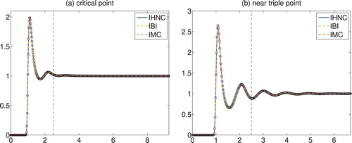
In both cases, the radial distribution function is sampled on an equidistant grid with mesh width $\Delta r=0.02$; for state point (a) we have data for m = 463 grid points covering a radial interval $r\in (0,9.26]$, for state point (b) we have m = 335 grid points within the interval $(0,6.7]$. The latter interval is smaller than the former one, because the density of the system is larger, and hence the simulation box is smaller. The given data are displayed as little circles in Figure 1. Note that the pair correlation function h = g−1 decays much faster at the critical point than near the triple point; as a consequence the inverse problem is much more difficult near the triple point.

Figure 1. Truncated and shifted Lennard–Jones fluids: radial distribution functions versus radius.

To solve the inverse problem, we have tabulated the approximate potentials on the first n = 125 grid points $r_i\in (0,2.5]$ of the same grid. Because of the particular definition of the IBI and IMC schemes, cf. (15(15) $u_{k+1}=u_k+\frac{1}{\beta }\log \frac{g_k}{g},g_k=G(u_k),$(15) ) and (16(16) $u_{k+1}=u_k+G^{\prime }(u_k{)}^{-1}(g-g_k),g_k=G(u_k),$(16) ), only those n grid points of the radial distribution function have been used for these two methods; this radial interval is indicated by the dashed lines in Figure 1. For IHNC, we have used the full data displayed in Figure 1. In all three iterative schemes, the same potential (24(24) $u_0=-\frac{1}{\beta }\log g,$(24) ) of mean force has been used as initial guess.

The approximate radial distribution functions obtained by IBI, IHNC and IMC, respectively, are also shown in Figure 1. Essentially, all three functions are on top of each other in both plots, and they constitute perfect fits of the given data for each of the two state points. But IHNC and IMC require far less iterations to achieve this goal: Figure 2 provides the corresponding iteration histories of the data fit, i.e. the graphs of the functions $k\mapsto \Vert G(u_k)-g{\Vert }_{\mathrm{\infty }}/\Vert G(u_0)-g{\Vert }_{\mathrm{\infty }}$ for all three individual iteration schemes and for each of the two state points, respectively; here, $\Vert G(u_k)-g{\Vert }_{\mathrm{\infty }}$ measures the maximal absolute error between all given measurement data and the corresponding approximations in the exterior of the core region. (For some obscure reason, this measure of the data fit is slightly increasing for IBI and IMC in the first iteration.) From these plots, it can be seen that IHNC requires about 5 iterations at the critical point and 11 iterations near the triple point to reach the global minimum of the data fit, while IMC requires 9 (or 5) iterations at the critical point and 7 iterations near the triple point; the data fit of the two methods is comparable, eventually. IBI, on the other hand, needs 10 iterations at the critical point and more than 20 near the triple point.

While the data fit is a straightforward indicator of the performance of the iterative schemes, the true error history is the really relevant quality measure. However, the latter is not available in practice. It is the advantage of this particular example that the true solution is known, so that the error history can be computed. For a particular potential $\tilde{u}$ given on the grid ${\mathrm{\Delta }}^{\prime }$, we define the error measure (40a) $ϵ(\tilde{u})={(\Delta r\sum _{i=1}^{n}g(r_i){(\tilde{u}(r_i)-u(r_i))}^2{r}_i^2)}^{1/2},$(40a) which approximates the weighted $L^2$ norm (40b) $ϵ(\tilde{u})\approx {({\int }_0^{\mathrm{\infty }}g(r){(\tilde{u}(r)-u(r))}^2{r}^2\mathrm{d}r)}^{1/2}$(40b) of the error $\tilde{u}-u$. This norm can be motivated by a more detailed analysis of the operator G, but this is beyond the scope of this paper; here we only emphasize that the factor g in (40b(40b) $ϵ(\tilde{u})\approx {({\int }_0^{\mathrm{\infty }}g(r){(\tilde{u}(r)-u(r))}^2{r}^2\mathrm{d}r)}^{1/2}$(40b) ) compensates for the divergence of the potentials as $r\to 0$.

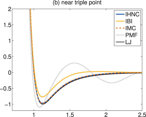
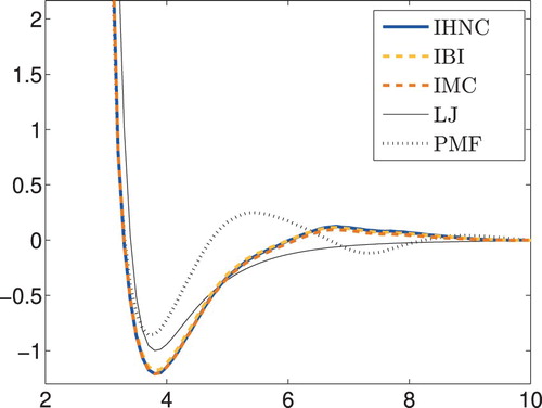
Figure 3 shows the relative error (41) $k\mapsto ϵ(u_k)/ϵ(u_0)$(41) as a function of the iteration count for all iterative schemes and both state points, respectively. The plots confirm that the particular iterates recommended above do indeed provide good approximations of the true truncated and shifted Lennard–Jones potential. Accordingly, IMC and IHNC both converge very rapidly in much the same number of iterations, whereas IBI is doing significantly worse. To illustrate this further the corresponding reconstructions for the more difficult problem near the triple point are shown in Figure 4. 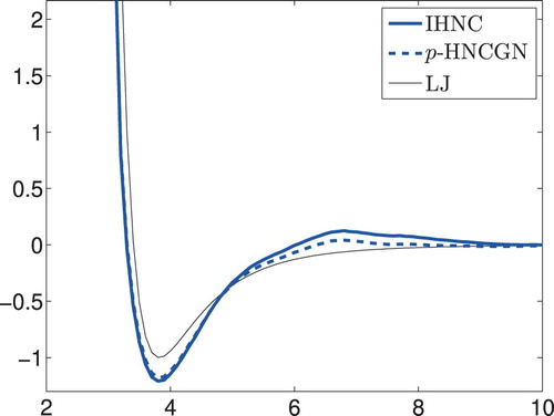This plot displays the 11th IHNC iterate, the 7th IMC iterate and the 50th (!) IBI iterate, together with the true pair potential as a black solid line (marked ‘LJ’) and the potential $u_0$ of mean force as a dotted line. As can be seen the IHNC and IMC approximations are hardly distinguishable from the true truncated and shifted Lennard–Jones potential, while even after 50 iterations IBI is still relatively far off.

7.2. Liquid argon

As a second example, we have determined approximate pair potentials for argon, using measurements by Schmidt and Tompson [30] for a state point with temperature $T=-{125}^{\circ }$ C and mass density $0.982\mathrm{g}/{\mathrm{cm}}^3$ in the liquid phase near the critical point.⁴ The corresponding data are given on an equidistant grid⁵ with m = 200 grid points and mesh width $\Delta r=0.1\text{Å}$. The approximate pair potentials have been tabulated on the first n = 100 grid points of this grid, and taken to be identically zero for $r>10\text{Å}$.

Figure 2. Truncated and shifted Lennard–Jones fluids: data fit versus iteration count.

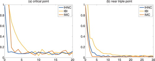
Figure 3. Truncated and shifted Lennard–Jones fluids: error (41(41) $k\mapsto ϵ(u_k)/ϵ(u_0)$(41) ) versus iteration count.

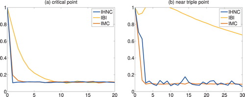
Figure 4. Truncated and shifted Lennard–Jones fluid: reconstructed pair potentials versus radius.

The iteration history shown in Figure 5 documents that, again, IHNC and IMC match the data much faster than IBI does: according to this plot 6 IHNC (5 IMC) iterations are sufficient, whereas IBI needs 39 iterations to achieve the same accuracy. Figure 6 presents the corresponding approximations of the radial distribution function and Figure 7 the corresponding potentials, together with the potential of mean force as dotted line. As before, all computed approximations are very close to each other.

Figure 5. Liquid argon: data fit versus iteration count.

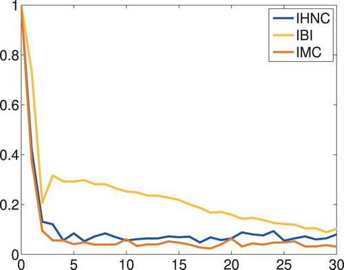
Figure 6. Liquid argon: radial distribution functions versus radius (in $\text{Å}$); detail view on the right.

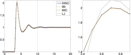
Figure 7. Liquid argon: approximate potentials (in units of ϵ) versus radius (in $\text{Å}$).

We have chosen argon as benchmark test case, because the interactions between argon atoms are widely considered to be well described by the Lennard–Jones pair potential (38(38) $u_{\mathrm{LJ}}=4\epsilon ((\sigma /r{)}^{12}-(\sigma /r{)}^6),r>0,$(38) ) with parameters $\sigma =3.405\text{Å}\mathrm{and}\epsilon =119.8k_{\mathrm{B}}\mathrm{J},$ cf., e.g. Tuckerman [31, p. 127]. This Lennard–Jones potential is given by the thin black line in Figure 7, but it differs quite a bit from our computed pair potentials. In fact, the radial distribution function corresponding to this Lennard–Jones approximation, which has also been included in Figure 6, does not fit the measured data well, as can easily be seen in the magnified detail in the right-hand plot. Even the initial approximation from the potential of mean force is doing better than that. So for this real-world example, we cannot trust this Lennard–Jones potential to be the ‘ground truth’ to compare our numerical results to.

7.3. The pressure constrained HNCGN scheme

Finally, we show some numerical results for p-HNCGN, i.e. the pressure constrained hypernetted-chain Gauss–Newton iteration described in Section 6. For this we have used the same data set for liquid argon as in the previous example and have imposed the corresponding value $p=9918.7\mathrm{kPa}$ of the pressure reported by Mikolaj and Pings [32].

Figures 8 and 9 present the corresponding numerical results. In the left-hand plot of Figure 8, we recollect the data fit history of Figure 5 and also show the corresponding graph for the performance of p-HNCGN: since the latter aims for a best possible fit of all 200 data points $g(r_j)$, it reaches a smaller value than all other competing methods.

Figure 8. Liquid argon: iteration history.

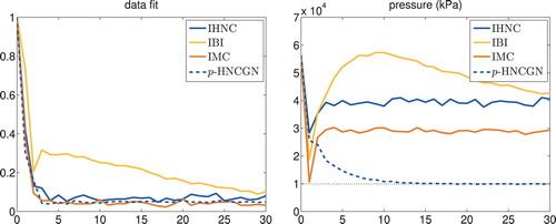
Figure 9. Liquid argon: approximate potentials (in units of ϵ) versus radius (in $\text{Å}$).

The right-hand plot of Figure 8, on the other hand, displays the average pressure (as returned by gromacs) of all corresponding ensembles for each individual iterate of the respective methods. The correct value of the pressure is indicated by the dotted horizontal line. As can be seen, except for p-HNCGN all methods fail to reproduce this number by a factor of 3 or more. p-HNCGN, on the other hand, achieves an excellent match of the target pressure after about 12 iterations.

Assessing both plots of Figure 8 we consider the 14th iterate of p-HNCGN to be ‘optimal’, because it corresponds to the first local minimum of the data fit after having reached a fairly accurate value of the pressure. The corresponding pair potential is compared in Figure 9 with the Lennard–Jones reference and the IHNC potential from Figure 7. It can be seen that the match of the pressure has a discernible (positive) impact on the computed pair potential.

Remark 7.1

Since p-HNCGN fits the data points of the measured radial distribution function, it does provide a good fit of the compressibility ${\kappa }_T$ of the fluid as well, because the compressibility is given by the Kirkwood–Buff integral $\frac{{\rho }_0}{\beta }{\kappa }_T=1+4\pi {\rho }_0{\int }_0^{\mathrm{\infty }}h(r)r^2\mathrm{d}r,$ which only depends on the pair correlation function h = g−1. Therefore p-HNCGN is able to fit both the compressibility and the pressure of a fluid to a reasonable accuracy. In the pertinent literature, this has been considered impossible when using isotropic pair potentials, compare, e.g. Wang, Junghans, and Kremer [26].

8. Conclusion

We have determined new generalized Newton schemes for the inverse Henderson problem, where we approximate the inverse of the Jacobian by the functional derivative of the hypernetted-chain approximation of the pair potential. These methods have about the same computational costs per iteration as IBI, but need much less iterations near phase transitions. In terms of iteration counts they are competitive to IMC, but the individual iterations are much cheaper than the IMC ones, because no cross-correlations need to be evaluated in the numerical simulation of the corresponding ensemble of particles. While these methods turn out to be similar (but not identical) to the LWR scheme of Levesque, Weis and Reatto, they are more flexible by construction, and can easily be modified, e.g. to also match the true pressure of the target ensemble.

We finally mention that one can also use the Percus–Yevick approximation instead of the hypernetted-chain approximation for the derivation of a corresponding generalized Newton method. The resulting scheme is very similar to (20(20) $u_{k+1}=u_k+\frac{1}{\beta }\log \frac{g_k}{g}+\frac{1}{\beta }{\phi }_k,k=0,1,2,\dots ,$(20) ), the only difference being that ${\phi }_k$ is replaced by ${\phi }_k/y_k$, where $y_k$ is the cavity distribution function associated with the kth pair potential $u_k$. In our numerical experiments, we found the iteration (20(20) $u_{k+1}=u_k+\frac{1}{\beta }\log \frac{g_k}{g}+\frac{1}{\beta }{\phi }_k,k=0,1,2,\dots ,$(20) ) to perform better near phase transitions of the truncated and shifted Lennard–Jones potentials than the corresponding Percus–Yevick recursion, and therefore we have restricted our attention to the IHNC scheme in this work.

In future work, we plan to extend our methods to binary mixtures of different fluids.

Acknowledgments

We are grateful to Gergely Tóth for pointing out to us references [7,12,17].

Disclosure statement

No potential conflict of interest was reported by the authors.

Additional information

Funding

This work was funded by the Deutsche Forschungsgemeinschaft (DFG, German Research Foundation) – Project number 233630050 - TRR 146.

Notes

1 We mention that this name may be misleading in that the approximate pair potential computed by IMC is not the result of some sophisticated Monte-Carlo simulation.

2 http://www.votca.org

3 For the core region the radius $r_0$ is chosen in each iteration as the smallest grid point of (28(28) $\mathrm{\Delta }=\{r_j=j\Delta r:j=1,\dots ,m\}$(28) ), such that g and $g_k$ are nonzero for every $r_j>r_0$.

4 According to the US National Institute of Standards and Technology the critical point of argon is located at about temperature $T=-{122.3}^{\circ }$ C and mass density $0.536\mathrm{g}/{\mathrm{cm}}^3$; see https://webbook.nist.gov/cgi/inchi?ID=C7440371&Mask=4.

5 For $r>10\text{Å}$ only every second data point is tabulated in [30]; the missing data have been filled in by linear interpolation.

Appendix

The Wiener lemma

Throughout this appendix we only consider functions of three variables, whether they be radial functions, or not. If $f\in L_{\varrho }^{\mathrm{\infty }}({\mathbb{R}}^3)$ is radially symmetric, then its representation defined in ${\mathbb{R}}^{+}$ belongs to the Banach space $L_{\varrho }^{\mathrm{\infty }}$ introduced in (5(5) $\Vert f{\Vert }_{L_{\varrho }^{\mathrm{\infty }}}=\Vert \varrho f{\Vert }_{(0,\mathrm{\infty })},$(5) ). The three-dimensional Fourier transform of $f\in L_{\varrho }^{\mathrm{\infty }}({\mathbb{R}}^3)$ is denoted by $\hat{f}$.

For ϱ defined in (4(4) $\varrho (r)=(1+r^2{)}^{\alpha /2},r\ge 0,$(4) ), we have shown in [11] that the space $L_{\varrho }^{\mathrm{\infty }}({\mathbb{R}}^3)$ of all functions $f:{\mathbb{R}}^3\to \mathbb{R}$, for which $\Vert f{\Vert }_{L_{\varrho }^{\mathrm{\infty }}({\mathbb{R}}^3)}={\mathrm{ess}\sup }_{R\in {\mathbb{R}}^3}\varrho (|R|)|f(R)|<\mathrm{\infty }$ constitutes a Banach algebra with respect to convolution. We can extend $L_{\varrho }^{\mathrm{\infty }}({\mathbb{R}}^3)$ to a Banach algebra ${\mathcal{W}}_{\varrho }$ with unit element e (given by the delta distribution at the origin), using the canonical norm $\Vert \lambda e+f{\Vert }_{{\mathcal{W}}_{\varrho }}=|\lambda |+\gamma \Vert f{\Vert }_{L_{\varrho }^{\mathrm{\infty }}({\mathbb{R}}^3)},\lambda \in \mathbb{R},f\in L_{\varrho }^{\mathrm{\infty }}({\mathbb{R}}^3),$ where $\gamma >0$ is a small enough constant to make the norm of ${\mathcal{W}}_{\varrho }$ submultiplicative.

The standard Wiener lemma for the Fourier transform starts with a similar construction for the Banach algebra $L^1({\mathbb{R}}^3)$ and states that if $f\in L^1({\mathbb{R}}^3)$ is such that $1+\hat{f}\ne 0$, then (A1) $(1+\hat{f}{)}^{-1}=1-\hat{c}$(A1) for some $c\in L^1({\mathbb{R}}^3)$ with Fourier transform $\hat{c}$, cf., e.g. Jörgens [8]. The weighted Wiener lemma which is required for the proof of Proposition 2.1 reads as follows.

Lemma A.1

Let $f\in L_{\varrho }^{\mathrm{\infty }}({\mathbb{R}}^3)$ be such that $1+\hat{f}\ne 0$. Then the function c of (A1(A1) $(1+\hat{f}{)}^{-1}=1-\hat{c}$(A1) ) belongs to $L_{\varrho }^{\mathrm{\infty }}({\mathbb{R}}^3)$. If f is a radial function, so is c.

Proof.

We choose u (not to mix up with the pair potential in the remainder of this paper) from the standard Schwartz space $\mathcal{S}$, sufficiently close to f in $L^1({\mathbb{R}}^3)$ so that $1+\hat{u}\ne 0$. Then we can apply the classical Wiener lemma to deduce that there exist $c,d\in L^1({\mathbb{R}}^3)$ which satisfy (A1(A1) $(1+\hat{f}{)}^{-1}=1-\hat{c}$(A1) ) and (A2) $(1+\hat{u}{)}^{-1}=1-\hat{d},$(A2) respectively. Moreover, $d\to c$ in $L^1({\mathbb{R}}^3)$ as $u\to f$ in $L^1({\mathbb{R}}^3)$; see [8]. Evidently, $\hat{d}=\frac{\hat{u}}{1+\hat{u}}\in \mathcal{S},$ and hence, $d\in \mathcal{S}$, and (A3) $w=(e-d)\ast (u-f)\in L_{\varrho }^{\mathrm{\infty }}({\mathbb{R}}^3)$(A3) with $\Vert w{\Vert }_{L^1({\mathbb{R}}^3)}\le (1+\Vert d{\Vert }_{L^1({\mathbb{R}}^3)})\Vert u-f{\Vert }_{L^1({\mathbb{R}}^3)}<1,$ provided u is sufficiently close to f. In (A3(A3) $w=(e-d)\ast (u-f)\in L_{\varrho }^{\mathrm{\infty }}({\mathbb{R}}^3)$(A3) ) and below the symbol $\ast$ refers to the standard three-dimensional convolution, i.e. $w(R)=u(R)-f(R)-{\int }_{{\mathbb{R}}^3}d(R-R^{\prime })(u(R^{\prime })-f(R^{\prime }))\mathrm{d}{R}^{\prime },R\in {\mathbb{R}}^3.$ Since $\Vert w{\Vert }_{L^1({\mathbb{R}}^3)}$ has been shown to be less than 1, Corollary 4.3 in [11] allows to conclude that the series (A4) $W_{\mathrm{\Sigma }}:=\sum _{n=1}^{\mathrm{\infty }}{W}_n$(A4) of the n-fold autoconvolutions $W_n$ of w converges in $L_{\varrho }^{\mathrm{\infty }}({\mathbb{R}}^3)$, and hence, $c_0:=d-W_{\mathrm{\Sigma }}+d\ast W_{\mathrm{\Sigma }}\in L_{\varrho }^{\mathrm{\infty }}({\mathbb{R}}^3).$ It turns out that this very function $c_0$ coincides with c, for we have ${\hat{c}}_0=\hat{d}-(1-\hat{d})\frac{\hat{w}}{1-\hat{w}}=\frac{\hat{d}-\hat{w}}{1-\hat{w}},$ and when inserting (A3(A3) $w=(e-d)\ast (u-f)\in L_{\varrho }^{\mathrm{\infty }}({\mathbb{R}}^3)$(A3) ) and (A2(A2) $(1+\hat{u}{)}^{-1}=1-\hat{d},$(A2) ) it follows that (A5) ${\hat{c}}_0=\frac{\hat{d}-(1-\hat{d})(\hat{u}-\hat{f})}{1-(1-\hat{d})(\hat{u}-\hat{f})}=\frac{\hat{u}-(\hat{u}-\hat{f})}{1+\hat{u}-(\hat{u}-\hat{f})}=\frac{\hat{f}}{1+\hat{f}}=\hat{c},$(A5) as has been claimed. This shows that $c\in L_{\varrho }^{\mathrm{\infty }}({\mathbb{R}}^3)$.

If f is a radial function, so is $\hat{f}$ and also $\hat{c}$ according to (A5(A5) ${\hat{c}}_0=\frac{\hat{d}-(1-\hat{d})(\hat{u}-\hat{f})}{1-(1-\hat{d})(\hat{u}-\hat{f})}=\frac{\hat{u}-(\hat{u}-\hat{f})}{1+\hat{u}-(\hat{u}-\hat{f})}=\frac{\hat{f}}{1+\hat{f}}=\hat{c},$(A5) ). Hence, c is a radial function, too.

Motivated by (A5(A5) ${\hat{c}}_0=\frac{\hat{d}-(1-\hat{d})(\hat{u}-\hat{f})}{1-(1-\hat{d})(\hat{u}-\hat{f})}=\frac{\hat{u}-(\hat{u}-\hat{f})}{1+\hat{u}-(\hat{u}-\hat{f})}=\frac{\hat{f}}{1+\hat{f}}=\hat{c},$(A5) ), we simply write (A6) $c=f\ast (e+f{)}^{-1}$(A6) for the solution c of (A1(A1) $(1+\hat{f}{)}^{-1}=1-\hat{c}$(A1) ) in the sequel. For the ease of completeness, we also include the following result on continuous dependence of $c\in L_{\varrho }^{\mathrm{\infty }}({\mathbb{R}}^3)$.

Lemma A.2

Let $f\in L_{\varrho }^{\mathrm{\infty }}({\mathbb{R}}^3)$ satisfy the assumptions of Lemma A.1, and let c be given by (A6(A6) $c=f\ast (e+f{)}^{-1}$(A6) ). If $f_k\in L_{\varrho }^{\mathrm{\infty }}({\mathbb{R}}^3)$ is sufficiently close to f in $L_{\varrho }^{\mathrm{\infty }}({\mathbb{R}}^3)$, then the Ornstein–Zernike relation (A1(A1) $(1+\hat{f}{)}^{-1}=1-\hat{c}$(A1) ) with f replaced by $f_k$ has a well-defined solution $c_k\in L_{\varrho }^{\mathrm{\infty }}({\mathbb{R}}^3)$, and there holds $\Vert c_k-c{\Vert }_{L_{\varrho }^{\mathrm{\infty }}({\mathbb{R}}^3)}\to 0\mathrm{as}\Vert f_k-f{\Vert }_{L_{\varrho }^{\mathrm{\infty }}({\mathbb{R}}^3)}\to 0.$

Proof.

We write $(e+f_k{)}^{-1}=(e+f{)}^{-1}\ast (e+w_k{)}^{-1}$ with (A7) $w_k=(e+f{)}^{-1}\ast (f_k-f),$(A7) and note that $\Vert w_k{\Vert }_{L^1({\mathbb{R}}^3)}\le q<1$ for $\Vert f_k-f{\Vert }_{L_{\varrho }^{\mathrm{\infty }}({\mathbb{R}}^3)}$ sufficiently small. Using (A1(A1) $(1+\hat{f}{)}^{-1}=1-\hat{c}$(A1) ) it follows that (A8) $\begin{array}{rl}{c}_k& =f_k\ast (e+f_k{)}^{-1}=f_k\ast (e+f{)}^{-1}\ast (e+w_k{)}^{-1}\\ & =f_k\ast (e-c)\ast (e+w_k{)}^{-1}=f_k\ast (e-c)\ast (e+W_{\mathrm{\Sigma },k})\\ & =f_k-f_k\ast c+(f_k-f_k\ast c)\ast W_{\mathrm{\Sigma },k},\end{array}$(A8) where $W_{\mathrm{\Sigma },k}$ is the series (A4(A4) $W_{\mathrm{\Sigma }}:=\sum _{n=1}^{\mathrm{\infty }}{W}_n$(A4) ) of the n-fold autoconvolutions of $w_k$. Note that (A9) $\Vert W_{\mathrm{\Sigma },k}{\Vert }_{L_{\varrho }^{\mathrm{\infty }}({\mathbb{R}}^3)}\le C\Vert w_k{\Vert }_{L_{\varrho }^{\mathrm{\infty }}({\mathbb{R}}^3)}$(A9) for some C>0 which only depends on the upper bound q of $\Vert w_k{\Vert }_{L^1({\mathbb{R}}^3)}$, cf. [11]. Rewriting c as $f\ast (e-c)$ by virtue of (A1(A1) $(1+\hat{f}{)}^{-1}=1-\hat{c}$(A1) ) and (A6(A6) $c=f\ast (e+f{)}^{-1}$(A6) ), we conclude from (A8(A8) $\begin{array}{rl}{c}_k& =f_k\ast (e+f_k{)}^{-1}=f_k\ast (e+f{)}^{-1}\ast (e+w_k{)}^{-1}\\ & =f_k\ast (e-c)\ast (e+w_k{)}^{-1}=f_k\ast (e-c)\ast (e+W_{\mathrm{\Sigma },k})\\ & =f_k-f_k\ast c+(f_k-f_k\ast c)\ast W_{\mathrm{\Sigma },k},\end{array}$(A8) ) that $c_k-c=f_k-f-(f_k-f)\ast c+(f_k-f_k\ast c)\ast W_{\mathrm{\Sigma },k},$ and hence, the assertion follows from (A9(A9) $\Vert W_{\mathrm{\Sigma },k}{\Vert }_{L_{\varrho }^{\mathrm{\infty }}({\mathbb{R}}^3)}\le C\Vert w_k{\Vert }_{L_{\varrho }^{\mathrm{\infty }}({\mathbb{R}}^3)}$(A9) ) and (A7(A7) $w_k=(e+f{)}^{-1}\ast (f_k-f),$(A7) ).

We finally mention that if h is the radially symmetric extension of the pair correlation function and if $f={\rho }_{0}h$, then $c/{\rho }_0$ coincides with the direct correlation function in the Ornstein-Zernike relation (8(8) $c+{\rho }_{0}h\ast c=h$(8) ); compare (A5(A5) ${\hat{c}}_0=\frac{\hat{d}-(1-\hat{d})(\hat{u}-\hat{f})}{1-(1-\hat{d})(\hat{u}-\hat{f})}=\frac{\hat{u}-(\hat{u}-\hat{f})}{1+\hat{u}-(\hat{u}-\hat{f})}=\frac{\hat{f}}{1+\hat{f}}=\hat{c},$(A5) ).

References

- Potestio R, Peter C, Kremer K. Computer simulations of soft matter: linking the scales. Entropy. 2014;16:4199–4245. doi: 10.3390/e16084199
- Henderson RL. A uniqueness theorem for fluid pair correlation functions. Phys Lett A. 1974;49:197–198. doi: 10.1016/0375-9601(74)90847-0
- Ben-Naim A. Molecular theory of solutions. New York: Oxford University Press; 2006.
- Hansen J-P, McDonald IR. Theory of simple liquids. 4th ed. Oxford: Academic Press; 2013.
- Mirzoev A, Lyubartsev AP. MagiC: software package for multiscale modeling. J Chem Theory Comput. 2013;9:1512–1520. doi: 10.1021/ct301019v
- Rühle V, Junghans C, Lukyanov A, et al. Versatile object-oriented toolkit for coarse-graining applications. J Chem Theory Comput. 2009;5:3211–3223. doi: 10.1021/ct900369w
- Tóth G. Interactions from diffraction data: historical and comprehensive overview of simulation assisted methods. J Phys Condens Matter. 2007;19:335220.
- Jörgens K. Linear integral operators. Boston: Pitman; 1982.
- Ruelle D. Statistical mechanics: rigorous results. New York: W.A. Benjamin Publ.; 1969.
- Hanke M. Fréchet differentiability of molecular distribution functions I. L∞ analysis. Lett Math Phys. 2018;108:285–306. doi: 10.1007/s11005-017-1009-0
- Hanke M. Well-posedness of the iterative Boltzmann inversion. J Stat Phys. 2018;170:536–553. doi: 10.1007/s10955-017-1944-2
- Schommers W. A pair potential for liquid rubidium from the pair correlation function. Phys Lett. 1973;43A:157–158. doi: 10.1016/0375-9601(73)90591-4
- Soper AK. Empirical potential Monte Carlo simulation of fluid structure. Chem Phys. 1996;202:295–306. doi: 10.1016/0301-0104(95)00357-6
- Lyubartsev AP, Laaksonen A. Calculation of effective interaction potentials from radial distribution functions: a reverse Monte Carlo approach. Phys Rev E. 1995;52:3730–3737. doi: 10.1103/PhysRevE.52.3730
- Murtola T, Falck E, Karttunen M, et al. Coarse-grained model for phospholipid/cholesterol bilayer employing inverse Monte Carlo with thermodynamic constraints. J Chem Phys. 2007;126:075101.
- Ivanizki D. Numerical analysis of the relation between interactions and structure in a molecular fluid. PhD Thesis. Johannes Gutenberg-Universität Mainz; 2015.
- Levesque D, Weis JJ, Reatto L. Pair interaction from structural data for dense classical liquids. Phys Rev Lett. 1985;54:451–454. doi: 10.1103/PhysRevLett.54.451
- Heinen M. Calculating particle pair potentials from fluid-state pair correlations: iterative Ornstein–Zernike inversion. J Comput Chem. 2018;39:1531–1543. doi: 10.1002/jcc.25225
- Henrici P. Applied and computational complex analysis. Vol. 3. New York: John Wiley & Sons; 1986.
- Abraham MJ, van der Spoel D, Lindahl E, et al. the Gromacs development team. Gromacs User Manual version 2016.3, www.gromacs.org (2017).
- Hess B, Kutzner C, van der Spoel D, et al. GROMACS 4: algorithms for highly efficient, load-balanced, and scalable molecular simulation. J Chem Theory Comput. 2008;4:435–447. doi: 10.1021/ct700301q
- Lyubartsev A, Mirzoev A, Chen L, et al Systematic coarse-graining of molecular models by the Newton inversion method. Faraday Discuss. 2010;144:43–56. doi: 10.1039/B901511F
- Fu CC, Kulkarni PM, Shell MS, et al. A test of systematic coarse-graining of molecular dynamics simulations: thermodynamic properties. J Chem Phys. 2012;137:164106.
- Jain S, Garde S, Kumar SK. Do inverse Monte Carlo algorithms yield thermodynamically consistent interaction potentials? Ind Eng Chem Res. 2006;45:5614–5618. doi: 10.1021/ie060042h
- Reith D, Pütz M, Müller-Plathe F. Deriving effective mesoscale potentials from atomistic simulations. J Comput Chem. 2003;24:1624–1636. doi: 10.1002/jcc.10307
- Wang H, Junghans C, Kremer K. Comparative atomistic and coarse-grained study of water: what do we lose by coarse-graining? Eur Phys J E. 2009;28:221–229. doi: 10.1140/epje/i2008-10413-5
- Björck Å. Numerical methods for least squares problems. Philadelphia: SIAM; 1996.
- Smit B. Phase diagrams of Lennard–Jones fluids. J Chem Phys. 1992;96:8639–8640. doi: 10.1063/1.462271
- Hansen J-P, Verlet L. Phase transitions of the Lennard–Jones system. Phys Rev. 1969;184:151–161. doi: 10.1103/PhysRev.184.151
- Schmidt PW, Tompson CW. X-ray scattering studies of simple fluids. In: Frisch HL and Salsburg ZW, editors. Simple Dense Fluids, New York: Academic Press; 1968. p. 31–110.
- Tuckerman ME. Statistical mechanics: theory and molecular simulation. Oxford: Oxford University Press; 2010.
- Mikolaj PG, Pings CJ. Structure of liquids. III. An X-ray diffraction study of fluid argon. J Chem Phys. 1967;46:1401–1411. doi: 10.1063/1.1840864