An efficient optimization methodology of respiration rate parameters coupled with transport properties in mass balances to describe modified atmosphere packaging systems

ABSTRACT

In this study, we aimed to describe a modern, efficient, and reproducible methodology to optimize respiration rate parameters coupled with transport properties in mass balances describing Modified atmosphere packaging (MAP) systems. We considered mass balances for three different respiration rate j film (exponential, competitive and uncompetitive Michaelis–Menten kinetics) coupled with transport properties for two different packaging films. Experiments were conducted to validate the methodology using grapes placed in a polypropylene container opened on the top and sealed with packaging films. The methodology relies on a numerical optimization procedure called the Trust-Region-Reflective algorithm. We determined the predictive capability of models using goodness-of-fit criteria and assessed parameter uncertainty through standard errors. We also calculated the first-order optimality measure and the relative change in the sum of squares to verify the convergence of the implemented algorithm. Results showed that the respiration rate parameters obtained with this methodology for the exponential model provided a better fit than for the other two models. The fitting for the kinetic models is not very suitable since we found that the normalized standard errors were rather high. In conclusion, the methodology is robust, and we expect that it serves as a tool for assessing MAP technology design.

Keywords:

• Model parameter estimation
• Trust-Region-Reflective algorithm
• respiration rate
• mass balance
• MAP systems

2010 Mathematics Subject Classifications:

• 62-07
• 62F10
• 62F07
• 62P30

Nomenclature

$P_{O_2}$	=	$O_2$ permeability, mol m${}^{-1}$ h${}^{-1}$ kPa${}^{-1}$
$P_{C{O}_2}$	=	$C{O}_2$ permeability, mol m${}^{-1}$ h${}^{-1}$ kPa${}^{-1}$
ℓ	=	Film thickness, m
$P_{C{O}_2}^{\mathrm{ext}}$	=	External $C{O}_2$ partial pressure, kPa
$P_{O_2}^{\mathrm{ext}}$	=	External $O_2$ partial pressure, kPa
V	=	Packaging headspace volume, m${}^3$
R	=	Universal gas constant, kPa m${}^3$ mol${}^{-1}$ K${}^{-1}$
T	=	Storage temperature, K
m	=	Product mass, kg
$R_{O_2}$	=	Respiration rate of $O_2$, mol kg${}^{-1}$ h${}^{-1}$
$R_{C{O}_2}$	=	Respiration rate of $C{O}_2$, mol kg${}^{-1}$ h${}^{-1}$
$A_1$	=	Maximum $O_2$ consumption rate in the exponential model, kg${}^{-1}$ h${}^{-1}$
$A_2$	=	$O_2$ inhibition rate in the exponential model, mol${}^{-1}$
K	=	Ratio between the respiration rates in the exponential model, dimensionless
$V_{\max }$	=	Kinetic constant for $O_2$ reaction rate in the MMC and MMU models, mol kg${}^{-1}$ h${}^{-1}$
$K_m$	=	Michaelis constant for half-reaction rate in the MMC and MMU models, mol
$k_c$	=	Competitive inhibition constant ($C{O}_2$) in the MMC model, mol
$k_u$	=	Uncompetitive inhibition constant ($C{O}_2$) in the MMU model, mol
$\mathbf{U}$	=	$(n_{O_2},n_{C{O}_2})$ vector of concentrations, mol
$\mathit{\theta }$	=	Parameters vector, unit of the corresponding parameter
${\mathit{\theta }}_U$	=	Upper bound for parameters vector, unit of the corresponding parameter
${\mathit{\theta }}_L$	=	Lower bound for parameters vector, unit of the corresponding parameter
$S({\mathit{\theta }}^j)$	=	Sum of squares or objective function, mol${}^2$
${\delta }_{\mathit{\theta }}^{(k)}$	=	Norm of the step at iteration k + 1, unit of the corresponding parameter
${\delta }_S^{(k)}$	=	Relative change in the sum of squares at iteration k + 1, dimensionless
$\mathbf{\nabla }$	=	Gradient operator with respect to $\mathit{\theta }$ variables, [unit of the corresponding parameter]${}^{-1}$
$({\tilde{\sigma }}^j{)}^2$	=	Variance of the residuals for j dataset, mol${}^2$
${\hat{\sigma }}^j$	=	Root mean square error for j dataset, mol
$R^{2,j}$	=	Coefficient of determination for j dataset, dimensionless
$Co{v}^j$	=	Covariance matrix for j dataset, [unit of the corresponding parameter]${}^2$
${\left({\chi }^j\right)}_{i,l}$	=	$(i,l)$-component of the sensitivity function for j dataset, mol [unit of the corresponding parameter]${}^{-1}$
$n_{C{O}_2}$	=	Number of mol $C{O}_2$ at time t, mol
$n_{O_2}$	=	Number of mol $O_2$ at time t, mol
S	=	Surface area of the film, m${}^2$
j	=	Superscript for each packaging film, j = 1 for PSF503 and j = 2 for PPCX
i	=	Subscript for experimental data, $i=1,\dots ,I$
k	=	Number of iterations of the optimization algorithm
I	=	Number of experimental data, I = 240
t	=	Time, h
${\hat{\mathit{\theta }}}^{\mathit{j}}$	=	Nonlinear least-squares estimator (nonlinear LSE) for j dataset, unit of the corresponding parameter
${\mathit{s}\mathit{e}}^j$	=	Standard errors for j dataset, unit of the corresponding parameter
${\mathit{n}\mathit{s}\mathit{e}}^j$	=	Normalized standard errors for j dataset, dimensionless
$({\mathit{\theta }}^j{)}^0$	=	Initial guess for optimizing modelling parameters for j dataset, unit of the corresponding parameter
${\mathbf{U}}_i^j$	=	Experimental concentration at time i for j film
$\mathbf{U}(i,{\mathit{\theta }}^j)$	=	Theoretical concentration at time i for j film
${\mathbf{U}}_i^j-\mathbf{U}(i,{\mathit{\theta }}^j)$	=	i-component of the residuals vector for j film, mol
${\mathit{\epsilon }}^j$	=	Gaussian noise, unit of the corresponding data or parameter
$\mathbf{\Sigma }$	=	Standard deviation of the Gaussian noise, unit of the corresponding data or parameter
${\hat{\mathit{\theta }}}^{j,p}$	=	Perturbed nonlinear LSE, unit of the corresponding parameter
${\left({\mathit{\theta }}^{j,p}\right)}^{(0)}$	=	Perturbed initial parameters vector, unit of the corresponding parameter
$E_{{\mathit{\theta }}^{j,p}}^R$	=	Relative error in the nonlinear LSE computed from perturbed data or perturbed initial parameters, dimensionless
$E_{{\left({\mathit{\theta }}^{j,p}\right)}^{(0)}}^R$	=	Relative error for the perturbed initial parameters, dimensionless
$E_{n_{O_2}^j}^R$	=	Relative error in the $O_2$ data computed from perturbed $O_2$ data, dimensionless
$E_{n_{C{O}_2}^j}^R$	=	Relative error in the $C{O}_2$ data computed from perturbed $C{O}_2$ data, dimensionless
${\delta }_{S,p}^{(k)}$	=	Relative change in the sum of squares evaluated at perturbed nonlinear LSE, dimensionless

1. Introduction

The respiration rate plays a significant role in the postharvest quality of fresh fruit and vegetables [1]. The deterioration rate in these products is proportional to the respiration rate [2]. For this reason, modifying the air composition in packaging headspace is necessary to reduce the respiration rate [3]. Modified atmosphere packaging (MAP) is the suitable technology to reach this target [4].

We must emphasize that a MAP system is a complex dynamical process in which the respiration rate and packaging transport properties of the packaging film have to be coupled in a mass balance for $O_2$ and $C{O}_2$ concentrations to accurately simulate underlying phenomena [5]. Due to the high biological variability of fresh products, respiration rate parameters are characterized by great uncertainty, and this has led researchers to obtain them by empirical formulae not based on first principles, which were proposed first by [6] who used the mass balance principle in MAP technology. Several empirical models have been developed to get the respiration rate; for example, polynomial models, exponential models, and Michaelis–Menten kinetic models; the authors in Refs [7,8] do a complete review of the models used for the respiration rate. In previous models, the respiration rate is considered to be independent of the packaging transport properties, and it is fitted to the empirical data through standard regression techniques. Then, this respiration rate is used in the mass balance to obtain the gas concentrations for fitting models to experimental data. There are few studies that address optimization of respiration rate parameters coupled with transport properties of the packaging film based on the mass balance principle; we highlight the reference [9]. These authors carried out parameter estimation of the respiration rate combined with gas balance; however, there is no clear explanation of methodology implementation. This is only referenced in an article dated in the late 1970s. Dealing with parameter uncertainty is an essential issue for a robust design of MAP technology which has only been addressed by [10]. These authors use the so-called interval analysis technique to study the impact of parameter uncertainty in a MAP model describing the evolution of gas composition inside packaging. However, the implementation of the technique is rather difficult to understand and reproduce; moreover, there is no mention of the optimization algorithm used, which makes it very difficult to use by the MAP technology-related community.

Parameter estimation involves solving the inverse problem: given a model and measurements of some state or output variables, the parameters that characterize the system, i.e. those producing a good fit of the model with the data, need to be identified [11]. This problem is difficult since no unique analytical or numerical solution is usually available [11]. Even if a unique solution was available, suitable initial guesses are required by optimization solvers to compute parameter estimates for fitting a model to experimental data [11]. From the previous discussion, the main goal of the present study was to describe a hybrid approach [12], i.e. a methodology that holistically mixes mathematical modelling and experimental design, which is required as it has been shown in literature for better understanding the studied system by fitting parameters of a given model with a specific scenario and for obtaining models with predictive capability. In particular, we aim to develop a modern, efficient, and reproducible methodology for optimization respiration rate parameters, whose implementation illustrated by collecting data from white table grapes stored in MAP using two packaging film types and three models for the respiration rate coupled to the transport properties of the films materials: exponential model, and Michaelis–Menten kinetic models with competitive and uncompetitive inhibition of $C{O}_2$. The methodology relies on a numeric procedure called the Trust-Region-Reflective optimization algorithm. At the same time, we compared the predictive power of each model using goodness-of-fit criteria and assessed parameter uncertainty through standard errors.

This article organizes as follows. In Section 2.1, we describe the experimental procedure to collect data associated with white table grapes stored in MAP, and in Section 2.2 mass balance principles for $O_2$ and $C{O}_2$ concentrations that we use in this work. In Section 2.3, the methodology that relies on a practical identifiability approach is fully described. To make that, we introduce practical identifiability techniques to carry out parameter estimation (Section2.3.2), to assess goodness-of-fit to data (Section2.3.3), as well as quantifying parameter uncertainty of the proposed mass balance models (Section 2.3.4). We illustrate in detail the methodology implementation by showing (in Section 3) and discussing (in Section 4) the results of the practical identifiability analysis to the proposed models for the collected data, and finally, in Section 5, we summarize and conclude.

2. Material and methods

2.1. Experimental procedure

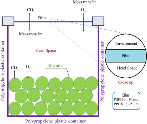
We purchased the table grapes in the organoleptic ripening state at the local market in Salerno, Italy. These bunches of grapes were immediately de-stemmed manually by cutting the stalk pedicel. Berries from bunches of grapes were then selected to obtain homogeneous samples in terms of colour, size, firmness, and defect- or disease-free. The samples of approximately 0.125 kg each (around 24 randomly selected berries per sample) were placed in six 1000 ${\mathrm{cm}}^3$ polypropylene plastic containers and one millimetre thick. With this thickness, from the experimental point of view, a negligible mass transfer can be considered in the container. Packaging headspace volume was calculated in three replicates as the difference between the total container volume and sample volume (5e−4 m${}^3$). The six containers were separated into lots of three (duplicated) and each batch was sealed at the top with a specific film. A packaging machine (Food Pack-Speedyn, ILPRA SpA, Mortara (PV), Italy) was used to thermally seal the three containers of each batch in the upper part with the specified films and an available surface of 4e−2 m${}^2$ was left for gas exchange. The films used for each lot were PSF530 (100% polyester film, with a thickness of 25 µ m), characterized by a high $O_2$ barrier (Sealed Air Global Italy Rho (MI), Italy) and PPCX (Polypropylene copolymer film, with a thickness of 35 µ m), characterized by a medium $O_2$ barrier (Carton Pack${}^{\circledR }$, Rutigliano (BA), Italy). Figure 1 depicts the two-dimensional cross-section of one of the containers. The selected packaging criterion was passive MAP (pMAP) [13], and the sealed containers were stored at 283 K.

Figure 1. Two-dimensional cross-section of the polypropylene container. The container is open at the top for allowing the mass transfer of $O_2$ and $C{O}_2$ through the film, whereas the other three sides are considered impervious, i.e. no mass transfer through them.

The headspace gas composition was periodically analysed to measure $O_2$ and $C{O}_2$ concentrations with a gas analyser (Servomex Mod. 1450 Food Package Analyzer, Crowborough, Sussex, UK) during 10 d of storage. The sample volume from the packaging headspace for gas analysis was approximately 10 cm${}^3$, which is substantial. For this reason, measurements were taken only every 24 h to avoid overly drastic deviations in headspace gas concentrations. Considering that there were 10 d of storage, the number of experimental points was only 10. To achieve better parameter estimation results, these 10 experimental points were extended by standard least-squares nonlinear regression to provide data in 240 points. 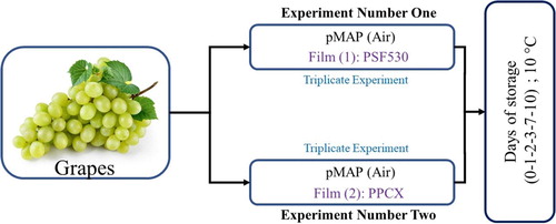The extended data was designated as $\{(n_{O_2}{)}_i^j,(n_{C{O}_2}{)}_i^j\}$ where the superscript j stands for each film type j $(j=1,\dots ,J$, where $J=2)$, whereas the subscript i denotes each datum at time i ($i=1,\dots ,I$ where I = 240 is the number of extended data for each j film). We must emphasize that the extension of the experimental data to obtain a larger dataset has nothing to do with the parameter estimation methodology, which is described and implemented in the present study. The extended data considered in the rest of the article corresponds to the mean of the extended data obtained in the three triplicated lots. The experimental schematic for each batch is shown in Figure 2.

Figure 2. Experimental schematic for pMAP of each lot stored in triplicate for the two films: PSF530 (25 µm thickness) and PPCX (35 µm thickness).

2.2. Mathematical modelling

In the present study, we considered different mass balance principles for $O_2$ and $C{O}_2$ concentrations, which described the time variation of these variables inside MAP during storage. Simpler models, which neglect spatial diffusion, are mathematical systems based on ordinary differential equation (ODE). These models can generally be stated as (1) $\begin{array}{rl}\frac{\mathrm{d}{n}_{O_2}}{\mathrm{d}t}& =\frac{S\cdot P_{O_2}}{\ell }(P_{O_2}^{\mathrm{ext}}-\frac{n_{O_2}\cdot R\cdot T}{V})-m\cdot R_{O_2}\end{array}$(1) (2) $\begin{array}{rl}\frac{\mathrm{d}{n}_{C{O}_2}}{\mathrm{d}t}& =\frac{S\cdot P_{C{O}_2}}{\ell }(P_{C{O}_2}^{\mathrm{ext}}-\frac{n_{C{O}_2}\cdot R\cdot T}{V})+m\cdot R_{C{O}_2}\end{array}$(2) The variables and parameters of the previous general mass balance principle are $n_{O_2}(t)$ (resp. $n_{C{O}_2}(t)$), which is the number of mol $O_2$ (resp. $C{O}_2$) at time t, S is the surface area of the film, $P_{O_2}$ is the $O_2$ permeability through each film, $P_{C{O}_2}$ is the $C{O}_2$ permeability through each film, ℓ is film thickness, $P_{O_2}^{\mathrm{ext}}$ is the external $O_2$ partial pressure, $P_{C{O}_2}^{\mathrm{ext}}$ is the external $C{O}_2$ partial pressure, V is the packaging headspace volume, R is the universal gas constant, T is the storage temperature, m is the product mass, and $R_{O_2}$ and $R_{C{O}_2}$ are the respiration rate of $O_2$ and $C{O}_2$, respectively. The values for the physical parameters and constants, which are independent of the film material and used in the mass balance (1(1) $\begin{array}{rl}\frac{\mathrm{d}{n}_{O_2}}{\mathrm{d}t}& =\frac{S\cdot P_{O_2}}{\ell }(P_{O_2}^{\mathrm{ext}}-\frac{n_{O_2}\cdot R\cdot T}{V})-m\cdot R_{O_2}\end{array}$(1) )–(2(2) $\begin{array}{rl}\frac{\mathrm{d}{n}_{C{O}_2}}{\mathrm{d}t}& =\frac{S\cdot P_{C{O}_2}}{\ell }(P_{C{O}_2}^{\mathrm{ext}}-\frac{n_{C{O}_2}\cdot R\cdot T}{V})+m\cdot R_{C{O}_2}\end{array}$(2) ), are displayed in Table 1.

Table 1. Physical parameters for general mass balance principle determined experimentally, except for the values of $P_{O_2}^{\mathrm{ext}}$, $P_{C{O}_2}^{\mathrm{ext}}$, and R that were obtained from the reference [14].

Parameter	Symbol	Value	Units
Area of package surface	S	4.0e−2	m${}^2$
External $O_2$ partial pressure	$P_{O_2}^{\mathrm{ext}}$	21	kPa
External $C{O}_2$ partial pressure	$P_{C{O}_2}^{\mathrm{ext}}$	3.5e−2	kPa
Package head space volume	V	5e−4	m${}^3$
Universal gas constant	R	8.3145e−3	kPa m${}^3$ mol${}^{-1}$ K${}^{-1}$
Storage temperature	T	283	K
Product mass	m	1.25e−1	Kg

The transport properties and film thickness are found in Table 2. These parameters were obtained from the technical specification sheet of each film.

Table 2. Parameters specific to each film type.

Parameter	Symbol	Unit	Film PSF530	Film PPCX
Thickness	ℓ	m	2.5e−5	3.5e−5
$O_2$ permeability	$P_{O_2}$	$O_2$ mol m${}^{-1}$ h${}^{-1}$ Kpa${}^{-1}$	6.9e−11	1.44e−9
$C{O}_2$ permeability	$P_{C{O}_2}$	$C{O}_2$ mol m${}^{-1}$ h${}^{-1}$ Kpa${}^{-1}$	7.67e−10	2.88e−9

The right-hand side of the mass balance (1(1) $\begin{array}{rl}\frac{\mathrm{d}{n}_{O_2}}{\mathrm{d}t}& =\frac{S\cdot P_{O_2}}{\ell }(P_{O_2}^{\mathrm{ext}}-\frac{n_{O_2}\cdot R\cdot T}{V})-m\cdot R_{O_2}\end{array}$(1) )–(2(2) $\begin{array}{rl}\frac{\mathrm{d}{n}_{C{O}_2}}{\mathrm{d}t}& =\frac{S\cdot P_{C{O}_2}}{\ell }(P_{C{O}_2}^{\mathrm{ext}}-\frac{n_{C{O}_2}\cdot R\cdot T}{V})+m\cdot R_{C{O}_2}\end{array}$(2) ) represents the respiration rate of fresh products combined with the gas flow through the film; it is expressed as the net rate at which $O_2$ and $C{O}_2$ concentrations change (mol h${}^{-1}$). The mass balance described by (1(1) $\begin{array}{rl}\frac{\mathrm{d}{n}_{O_2}}{\mathrm{d}t}& =\frac{S\cdot P_{O_2}}{\ell }(P_{O_2}^{\mathrm{ext}}-\frac{n_{O_2}\cdot R\cdot T}{V})-m\cdot R_{O_2}\end{array}$(1) )–(2(2) $\begin{array}{rl}\frac{\mathrm{d}{n}_{C{O}_2}}{\mathrm{d}t}& =\frac{S\cdot P_{C{O}_2}}{\ell }(P_{C{O}_2}^{\mathrm{ext}}-\frac{n_{C{O}_2}\cdot R\cdot T}{V})+m\cdot R_{C{O}_2}\end{array}$(2) ) has to be complemented with initial conditions for both variables, i.e. it mathematically corresponds to an initial value problem: (3) $\begin{array}{rl}{n}_{O_2}(t_0)& =n_{O_{2}0}\end{array}$(3) (4) $\begin{array}{rl}{n}_{C{O}_2}(t_0)& =n_{C{O}_{2}0}\end{array}$(4) In the present study, we considered three model types for the respiration rates $R_{O_2}$ and $R_{C{O}_2}$ at the right-hand side of the mass balance given by (1(1) $\begin{array}{rl}\frac{\mathrm{d}{n}_{O_2}}{\mathrm{d}t}& =\frac{S\cdot P_{O_2}}{\ell }(P_{O_2}^{\mathrm{ext}}-\frac{n_{O_2}\cdot R\cdot T}{V})-m\cdot R_{O_2}\end{array}$(1) )–(2(2) $\begin{array}{rl}\frac{\mathrm{d}{n}_{C{O}_2}}{\mathrm{d}t}& =\frac{S\cdot P_{C{O}_2}}{\ell }(P_{C{O}_2}^{\mathrm{ext}}-\frac{n_{C{O}_2}\cdot R\cdot T}{V})+m\cdot R_{C{O}_2}\end{array}$(2) ). The first model is a modification of the one used by [9], referred to as the exponential model, and states that the respiration rate terms are described by the following equations: (5) $\begin{array}{rl}{R}_{O_2}& =A_1\cdot n_{O_2}\cdot \exp (-A_2\cdot n_{C{O}_2})\end{array}$(5) (6) $\begin{array}{rl}{R}_{C{O}_2}& =K{R}_{O_2}=K\cdot A_1\cdot n_{O_2}\cdot \exp (-A_2\cdot n_{C{O}_2})\end{array}$(6) The parameters to be estimated in the model (1(1) $\begin{array}{rl}\frac{\mathrm{d}{n}_{O_2}}{\mathrm{d}t}& =\frac{S\cdot P_{O_2}}{\ell }(P_{O_2}^{\mathrm{ext}}-\frac{n_{O_2}\cdot R\cdot T}{V})-m\cdot R_{O_2}\end{array}$(1) )–(2(2) $\begin{array}{rl}\frac{\mathrm{d}{n}_{C{O}_2}}{\mathrm{d}t}& =\frac{S\cdot P_{C{O}_2}}{\ell }(P_{C{O}_2}^{\mathrm{ext}}-\frac{n_{C{O}_2}\cdot R\cdot T}{V})+m\cdot R_{C{O}_2}\end{array}$(2) ) for the respiration rates $R_{O_2}$ and $R_{C{O}_2}$ (mol kg${}^{-1}$ h${}^{-1}$) defined by (5(5) $\begin{array}{rl}{R}_{O_2}& =A_1\cdot n_{O_2}\cdot \exp (-A_2\cdot n_{C{O}_2})\end{array}$(5) ) and (6(6) $\begin{array}{rl}{R}_{C{O}_2}& =K{R}_{O_2}=K\cdot A_1\cdot n_{O_2}\cdot \exp (-A_2\cdot n_{C{O}_2})\end{array}$(6) ), respectively, are grouped in the vector $\mathit{\theta }=(A_1,A_2,K)\in {\mathbb{R}}^3$. The parameters in the vector $\mathit{\theta }$ are $A_1$ that stands for the maximum $O_2$ consumption rate (kg${}^{-1}$ h${}^{-1}$), $A_2$ that denotes the $C{O}_2$ inhibition factor (mol${}^{-1}$), and K that represents the ratio between the respiration rates (dimensionless). The exponential model is a modification of the Michaelis–Menten model that considers competitive inhibition of $O_2$ at high $C{O}_2$ concentrations.

The second and third models of the present study consist in assuming that the role of $C{O}_2$ in respiration is mediated by competitive and uncompetitive inhibition mechanisms of the Michaelis–Menten type [7]. In the first case, the maximum respiration rate of $O_2$ is influenced at high $C{O}_2$ concentrations, whereas in the second case, $O_2$ is not influenced by $C{O}_2$; these models are referred to as competitive Michaelis–Menten (MMC) and uncompetitive Michaelis–Menten (MMU). These mathematical models for the respiration rates $R_{O_2}$ and $R_{C{O}_2}$ are defined by the following equations: (7) $\begin{array}{rl}{R}_{O_2}& =\frac{V_{max}\cdot n_{O_2}}{K_m+n_{O_2}}\end{array}$(7) (8) $\begin{array}{rl}{R}_{C{O}_2}& =100\frac{V_{max}\cdot n_{O_2}}{n_{O_2}+K_m\cdot (1+{\displaystyle \frac{n_{C{O}_2}}{K_c}})}\end{array}$(8) (9) $\begin{array}{rl}{R}_{C{O}_2}& =100\frac{V_{max}\cdot n_{O_2}}{K_m+n_{O_2}\cdot (1+{\displaystyle \frac{n_{C{O}_2}}{K_u}})}\end{array}$(9) The MMC model corresponds to the respiration rates $R_{O_2}$ and $R_{C{O}_2}$ defined by (7(7) $\begin{array}{rl}{R}_{O_2}& =\frac{V_{max}\cdot n_{O_2}}{K_m+n_{O_2}}\end{array}$(7) ) and (8(8) $\begin{array}{rl}{R}_{C{O}_2}& =100\frac{V_{max}\cdot n_{O_2}}{n_{O_2}+K_m\cdot (1+{\displaystyle \frac{n_{C{O}_2}}{K_c}})}\end{array}$(8) ), respectively, where the kinetic parameters are grouped in the vector $\mathit{\theta }=(V_{\max },K_m,K_c)\in {\mathbb{R}}^3$. On the other hand, the MMU model corresponds to the respiration rates $R_{O_2}$ and $R_{C{O}_2}$ defined by (7(7) $\begin{array}{rl}{R}_{O_2}& =\frac{V_{max}\cdot n_{O_2}}{K_m+n_{O_2}}\end{array}$(7) ) and (9(9) $\begin{array}{rl}{R}_{C{O}_2}& =100\frac{V_{max}\cdot n_{O_2}}{K_m+n_{O_2}\cdot (1+{\displaystyle \frac{n_{C{O}_2}}{K_u}})}\end{array}$(9) ), respectively, where the kinetic parameters are grouped in the vector $\mathit{\theta }=(V_{\max },K_m,K_u)\in {\mathbb{R}}^3$. For MMC and MMU models, the parameters in the vector $\mathit{\theta }$ are $V_{\max }$ that stands for the maximum $O_2$ consumption (mol kg${}^{-1}$ h${}^{-1}$), $K_m$ that denotes the oxygen concentration at which the reaction rate is half of $V_{\max }$ ($O_2$ mol), $K_c$ and $K_u$ stand for the competitive and uncompetitive inhibition constants ($C{O}_2$ mol), respectively.

The respiration rate $R_{O_2}$ for the exponential model defined in (5(5) $\begin{array}{rl}{R}_{O_2}& =A_1\cdot n_{O_2}\cdot \exp (-A_2\cdot n_{C{O}_2})\end{array}$(5) ) is obtained by linearizing $R_{O_2}$ defined in Equation (7(7) $\begin{array}{rl}{R}_{O_2}& =\frac{V_{max}\cdot n_{O_2}}{K_m+n_{O_2}}\end{array}$(7) ), which results in $R_{O_2}=A\cdot n_{O_2}$ where $A=A_1\exp (-A_2\cdot n_{C{O}_2})$ takes into account competitive inhibition of the $O_2$ respiration rate when the $C{O}_2$ concentration is high, because $R_{O_2}$ decreases when the $C{O}_2$ concentration increases at high values according to Equation (5(5) $\begin{array}{rl}{R}_{O_2}& =A_1\cdot n_{O_2}\cdot \exp (-A_2\cdot n_{C{O}_2})\end{array}$(5) ). For all the models, the respiration rates of $O_2$ and $C{O}_2$, $R_{O_2}$ and $R_{C{O}_2}$, respectively, depend on parameters that were grouped in a vector $\mathit{\theta }\in {\mathbb{R}}^3$. We designated this dependence by $R_{O_2}(\mathit{\theta })$ and $R_{C{O}_2}(\mathit{\theta })$.

2.3. Identifiability analysis of modelling parameters

Mathematical models described in the previous section can be written under the general (vector) form as (10) $\begin{array}{rl}\frac{\mathrm{d}\mathbf{U}}{\mathrm{d}t}& =\mathbf{F}(\mathbf{U},\mathit{\theta })\end{array}$(10) (11) $\begin{array}{rl}\mathbf{U}(t_0)& ={\mathbf{U}}_0\end{array}$(11) where $\mathbf{U}:[t_0,t_f]\to {\mathbb{R}}^2$ is the vector of the MAP system state variables given by $\mathbf{U}(t)=(n_{O_2}(t),n_{C{O}_2}(t))$ for all $t\in [t_0,t_f]$, $t_0$ is the initial time, $t_f$ a sufficiently long time so as to let the system evolve, ${\mathbf{U}}_0=(n_{O_2,0},n_{C{O}_2,0})$ is the initial state, and $\mathbf{F}(\mathbf{U},\mathit{\theta })$ is defined by (12) $\begin{array}{rl}\mathbf{F}(\mathbf{U},\mathit{\theta })& =(\frac{S\cdot P_{O_2}}{\ell }(P_{O_2}^{\mathrm{ext}}-\frac{n_{O_2}\cdot R\cdot T}{V})-m\cdot R_{O_2}(\mathit{\theta }),\\ & \frac{S\cdot P_{C{O}_2}}{\ell }(P_{C{O}_2}^{\mathrm{ext}}-\frac{n_{C{O}_2}\cdot R\cdot T}{V})+m\cdot R_{C{O}_2}(\mathit{\theta }))\end{array}$(12) and corresponds to the right-hand side of the ODE system given by Equations (1(1) $\begin{array}{rl}\frac{\mathrm{d}{n}_{O_2}}{\mathrm{d}t}& =\frac{S\cdot P_{O_2}}{\ell }(P_{O_2}^{\mathrm{ext}}-\frac{n_{O_2}\cdot R\cdot T}{V})-m\cdot R_{O_2}\end{array}$(1) )–(2(2) $\begin{array}{rl}\frac{\mathrm{d}{n}_{C{O}_2}}{\mathrm{d}t}& =\frac{S\cdot P_{C{O}_2}}{\ell }(P_{C{O}_2}^{\mathrm{ext}}-\frac{n_{C{O}_2}\cdot R\cdot T}{V})+m\cdot R_{C{O}_2}\end{array}$(2) ). With this notation, we obtain each of the studied models by replacing the corresponding respiration rates $R_{O_2}(\mathit{\theta })$ and $R_{C{O}_2}(\mathit{\theta })$ in $\mathbf{F}(\mathbf{U},\mathit{\theta })$ along with the parameters vector $\mathit{\theta }$. For example, the exponential model is obtained by replacing $R_{O_2}(\mathit{\theta })$ and $R_{C{O}_2}(\mathit{\theta })$ as defined in Equation (5(5) $\begin{array}{rl}{R}_{O_2}& =A_1\cdot n_{O_2}\cdot \exp (-A_2\cdot n_{C{O}_2})\end{array}$(5) ) and (6(6) $\begin{array}{rl}{R}_{C{O}_2}& =K{R}_{O_2}=K\cdot A_1\cdot n_{O_2}\cdot \exp (-A_2\cdot n_{C{O}_2})\end{array}$(6) ) with $\mathit{\theta }=(A_1,A_2,K)\in {\mathbb{R}}^3$.

2.3.1. Direct and inverse problem

Given a parameters vector $\mathit{\theta }\in {\mathbb{R}}^3$, the direct problem consists of finding the (unique) solution $\mathbf{U}(t,\mathit{\theta })=(n_{O_2}(t,\mathit{\theta }),n_{C{O}_2}(t,\mathit{\theta }))$ of the mathematical model given by Equations (10(10) $\begin{array}{rl}\frac{\mathrm{d}\mathbf{U}}{\mathrm{d}t}& =\mathbf{F}(\mathbf{U},\mathit{\theta })\end{array}$(10) )–(11(11) $\begin{array}{rl}\mathbf{U}(t_0)& ={\mathbf{U}}_0\end{array}$(11) ). The solution to the direct problem is required to solve the inverse problem. The present study aimed to develop a clear, reproducible, and modern methodology to solve the parameter identification problem and compare the fit performance of different mathematical models to experimental data in such a way as to be able to decide which model best fits a given dataset. This procedure is referred to as the inverse problem, i.e. given experimental data that measures the vector $\mathbf{U}(t)=(n_{O_2}(t),n_{C{O}_2}(t))$ of concentrations at some time points to identify the parameters vector $\mathit{\theta }\in {\mathbb{R}}^3$ such that the mathematical model given by Equations (10(10) $\begin{array}{rl}\frac{\mathrm{d}\mathbf{U}}{\mathrm{d}t}& =\mathbf{F}(\mathbf{U},\mathit{\theta })\end{array}$(10) )–(11(11) $\begin{array}{rl}\mathbf{U}(t_0)& ={\mathbf{U}}_0\end{array}$(11) ) fits the data in the sense of the least-squares. More precisely, to solve the inverse problem of parameter estimation, it is necessary to find the vector ${\mathit{\theta }}^j\in {\mathbb{R}}^3$ so that the sum of squares (13) $S({\mathit{\theta }}^j)={\displaystyle \sum _{i=1}^I\Vert {\mathbf{U}}_i^j-\mathbf{U}(i,{\mathit{\theta }}^j){\Vert }^2}$(13)

is minimized, where (14) ${\mathbf{U}}_i^j=((n_{O_2}{)}_i^j,(n_{C{O}_2}{)}_i^j),\mathbf{U}(i,{\mathit{\theta }}^j)=(n_{O_2}(i,{\mathit{\theta }}^j),n_{C{O}_2}(i,{\mathit{\theta }}^j))$(14) at times $i=1,\dots ,I$, and for each dataset j = 1, 2. The objective function defined in (13(13) $S({\mathit{\theta }}^j)={\displaystyle \sum _{i=1}^I\Vert {\mathbf{U}}_i^j-\mathbf{U}(i,{\mathit{\theta }}^j){\Vert }^2}$(13) ) corresponds to the sum of squares of the residuals ${\mathbf{U}}_i^j-\mathbf{U}(i,{\mathit{\theta }}^j)$, i.e. of the differences between the experimental concentrations ${\mathbf{U}}_i^j$ and the theoretical concentrations $\mathbf{U}(i,{\mathit{\theta }}^j)$ given in (14(14) ${\mathbf{U}}_i^j=((n_{O_2}{)}_i^j,(n_{C{O}_2}{)}_i^j),\mathbf{U}(i,{\mathit{\theta }}^j)=(n_{O_2}(i,{\mathit{\theta }}^j),n_{C{O}_2}(i,{\mathit{\theta }}^j))$(14) ), where $\mathbf{U}(i,{\mathit{\theta }}^j)$ corresponds to the $O_2$ and $C{O}_2$ concentrations obtained from each model evaluated at $(i,{\mathit{\theta }}^j)$ at times $i=1,\dots ,I$ and for a given value of the parameters vector ${\mathit{\theta }}^j$.

The minimum of sum of squares $S({\mathit{\theta }}^{\mathit{j}})$ is designated as ${\hat{\mathit{\theta }}}^{\mathit{j}}$ for each dataset j = 1, 2. The vector ${\hat{\mathit{\theta }}}^{\mathit{j}}$ is called nonlinear least-squares estimator, hereafter denoted as nonlinear LSE. To minimize $S({\mathit{\theta }}^j)$ we used the Trust-Region-Reflective algorithm implemented in Matlab${}^{\circledR }$ under the subroutine lsqnonlin.

To assess the quality of the optimal solution ${\hat{\mathit{\theta }}}^{\mathit{j}}$, we also computed some metrics that allowed us to evaluate convergence associated with the algorithm, as well as a stopping criterion necessary to exit from it. The details to implement the lsqnonlin solver are discussed in Section 2.3.2. Once the nonlinear LSE (${\hat{\mathit{\theta }}}^{\mathit{j}}$) was found for each dataset j = 1, 2 and for each proposed model (exponential, MMU and MMC), we compared the three models for their data fit performance. This was achieved by computing a number of goodness-of-fit criteria, which are explained in Section 2.3.3. Finally, we computed the standard errors associated with the nonlinear LSE to assess parameter uncertainty as explained in Section 2.3.4.

2.3.2. Parameter estimation

The numerical algorithm used to optimize the objective function defined in Equation (13(13) $S({\mathit{\theta }}^j)={\displaystyle \sum _{i=1}^I\Vert {\mathbf{U}}_i^j-\mathbf{U}(i,{\mathit{\theta }}^j){\Vert }^2}$(13) ) is described in the present subsection and summarized, as well as schematized in Section 2.3.5.

We used the Trust-Region Interior Reflective (TIR) method, which was developed in [15], to minimize $S({\mathit{\theta }}^j)$ in Equation (13(13) $S({\mathit{\theta }}^j)={\displaystyle \sum _{i=1}^I\Vert {\mathbf{U}}_i^j-\mathbf{U}(i,{\mathit{\theta }}^j){\Vert }^2}$(13) ). Convergence is theoretically achieved under general conditions. However, the initial parameter estimate usually has to be close to the optimal solution to obtain convergence. Our models are simple to handle because their right-hand sides are autonomous (independent on time), formed by a negative exponential or a rational function (quotients of polynomials) at the variables, and depend on the parameters in a very regular way. The solution $(n_{O_2}(t,\mathit{\theta }),n_{C{O}_2}(t,\mathit{\theta }))$ systematically depends on the parameters vector $\mathit{\theta }$; in particular, it can be proven that it is infinitely differentiable with respect to $\mathit{\theta }$. We were able to efficiently minimize the objective function in Equation (13(13) $S({\mathit{\theta }}^j)={\displaystyle \sum _{i=1}^I\Vert {\mathbf{U}}_i^j-\mathbf{U}(i,{\mathit{\theta }}^j){\Vert }^2}$(13) ) with these good properties. We used the lsqnonlin solver implemented in Matlab${}^{\circledR }$ [16] with the TIR method, which is especially adapted for solving nonlinear least-squares minimization problems.

To make so, we have to evaluate the objective function $S({\mathit{\theta }}^j)$, which requires to solve the direct problem, i.e. to compute the numerical solution of the initial value problem given by Equations (10(10) $\begin{array}{rl}\frac{\mathrm{d}\mathbf{U}}{\mathrm{d}t}& =\mathbf{F}(\mathbf{U},\mathit{\theta })\end{array}$(10) )–(11(11) $\begin{array}{rl}\mathbf{U}(t_0)& ={\mathbf{U}}_0\end{array}$(11) ) or the ODE system given by Equations (1(1) $\begin{array}{rl}\frac{\mathrm{d}{n}_{O_2}}{\mathrm{d}t}& =\frac{S\cdot P_{O_2}}{\ell }(P_{O_2}^{\mathrm{ext}}-\frac{n_{O_2}\cdot R\cdot T}{V})-m\cdot R_{O_2}\end{array}$(1) )–(2(2) $\begin{array}{rl}\frac{\mathrm{d}{n}_{C{O}_2}}{\mathrm{d}t}& =\frac{S\cdot P_{C{O}_2}}{\ell }(P_{C{O}_2}^{\mathrm{ext}}-\frac{n_{C{O}_2}\cdot R\cdot T}{V})+m\cdot R_{C{O}_2}\end{array}$(2) ), which is the same, with initial conditions defined by Equations (3(3) $\begin{array}{rl}{n}_{O_2}(t_0)& =n_{O_{2}0}\end{array}$(3) )–(4(4) $\begin{array}{rl}{n}_{C{O}_2}(t_0)& =n_{C{O}_{2}0}\end{array}$(4) ) at times $i=1,\dots ,I$ for different parameters vectors ${\mathit{\theta }}^j$ depending on each dataset j = 1, 2. The initial conditions were established as the first measurement taken for each experiment to reproduce the real behaviour of $O_2$ and $C{O}_2$ concentrations, i.e. for each j = 1, 2 we defined ${\mathbf{U}}_0={\mathbf{U}}_1^j=((n_{O_2}{)}_1^j,(n_{C{O}_2}{)}_1^j)$ at time $t_1=1$ h in which the first extended datum was computed from the experimental data (Section 2.1). We computed the numerical solution of the direct problem using the ode45 Matlab${}^{\circledR }$ solver, which is based on an explicit Runge–Kutta type formula [17].

For every dataset j = 1, 2, the input arguments that we used for the lsqnonlin subroutine are provided in Table 3.

Table 3. Input arguments for lsqnonlin solver.

Description	Input argument
Residuals vector	${\mathbf{U}}_i^j-\mathbf{U}(i,{\mathit{\theta }}^{\mathit{j}})i=1,\dots ,I.$
Initial parameters vector	$({\mathit{\theta }}^{\mathit{j}}{)}^0$
Lower bound for parameters vector	${\mathit{\theta }}_L=(0,0,0)$
Upper bound for parameters vector	${\mathit{\theta }}_U=+\mathrm{\infty }\cdot (1,1,1)$

Moreover, we used the following options in the lsqnonlin solver from Matlab${}^{\circledR }$. Firstly, we chose the TIR method as the optimization algorithm, which is the default. Secondly, the maximum number of iterations was set at 10,000, while the maximum number of function evaluations was set at 20,000. Finally, the function tolerance and the norm of the step tolerance were both set at 1$e-$17. The norm of the step ${\delta }_{\mathit{\theta }}^{(k)}>0$ measures the change between two successive iterates ${\mathit{\theta }}^{(k)}$ and ${\mathit{\theta }}^{(k+1)}$, which is defined as (15) ${\delta }_{\mathit{\theta }}^{(k)}=\Vert {\mathit{\theta }}^{(k+1)}-{\mathit{\theta }}^{(k)}\Vert$(15) On the other hand, (16) ${\delta }_S^{(k)}=\frac{|S({\mathit{\theta }}^{(k)})-S({\mathit{\theta }}^{(k+1)})|}{1+|S({\mathit{\theta }}^{(k)})|}$(16) is the relative change in the sum of squares. The stopping criterion for our algorithm is defined as (17) $min\{{\delta }_{\mathit{\theta }}^{(k)},{\delta }_S^{(k)}\}<1e-17$(17) When the previous condition is met, the algorithm stops at iteration k + 1 and returns an approximation of the nonlinear LSE ${\hat{\mathit{\theta }}}^j:={\mathit{\theta }}^{(k+1)}$, as well as an approximation of the Jacobian matrix ${\chi }^j$ evaluated at $(i,{\hat{\mathit{\theta }}}^j)$ for each dataset j = 1, 2; see Section 2.3.4 for details. To check the convergence of the algorithm, we also provided the first-order optimality measure, which measures how close the approximation is to the actual minimum of the sum of squares. The first-order optimality measure is defined as the infinity norm of the gradient of the objective function evaluated at the nonlinear LSE ${\hat{\mathit{\theta }}}^{\mathit{j}}$, i.e. the optimal solution that approximately minimizes $S({\mathit{\theta }}^j)$, which in turn is given by the maximum absolute value of the partial derivatives of the objective function with respect to the $\mathit{\theta }$ variables: (18) $\Vert \mathbf{\nabla }S({\hat{\mathit{\theta }}}^j){\Vert }_{\mathrm{\infty }}=\underset{\ell =1,2,3}{max}|\frac{\mathrm{\partial }S}{\mathrm{\partial }{\mathit{\theta }}_{\ell }^j}({\hat{\mathit{\theta }}}^j)|$(18) Other metrics that quantify convergence are the relative change in the sum of squares ${\delta }_S^{(k)}$ (Equation (16(16) ${\delta }_S^{(k)}=\frac{|S({\mathit{\theta }}^{(k)})-S({\mathit{\theta }}^{(k+1)})|}{1+|S({\mathit{\theta }}^{(k)})|}$(16) )), the norm of the step ${\delta }_{\mathit{\theta }}^{(k)}$ (Equation (15(15) ${\delta }_{\mathit{\theta }}^{(k)}=\Vert {\mathit{\theta }}^{(k+1)}-{\mathit{\theta }}^{(k)}\Vert$(15) )), and the number of iterations k + 1. The metrics $\Vert \mathbf{\nabla }S({\hat{\mathit{\theta }}}^j){\Vert }_{\mathrm{\infty }},{\delta }_S^{(k)},{\delta }_{\mathit{\theta }}^{(k)}$ and k + 1 are displayed for the lsqnonlin solver at the end of its execution.

2.3.3. Goodness-of-fit criteria

We used statistical methods (from the context of nonlinear least-squares regression) to quantify the fit performance of each model with respect to data. More precisely, once the nonlinear LSE ${\hat{\mathit{\theta }}}^j$ was found for each dataset j = 1, 2 and for each proposed model, a number of goodness-of-fit criteria can be computed, which evaluate to what extent these models are fitted to each dataset. We computed $({\tilde{\sigma }}^j{)}^2,{\hat{\sigma }}^j,R^{2,j}$, i.e. the variance of the residuals, the root mean square error (RMSE), and the coefficient of determination, respectively, and which are given by [18,19]: (19) $\begin{array}{rl}({\tilde{\sigma }}^j{)}^2& =\frac{S({\hat{\mathit{\theta }}}^j)}{I}\end{array}$(19) (20) $\begin{array}{rl}{\hat{\sigma }}^j& =\sqrt{\frac{1}{I-3}S({\hat{\mathit{\theta }}}^j)}\end{array}$(20) (21) $\begin{array}{rl}{R}^{2,j}& =1-\frac{S({\hat{\mathit{\theta }}}^j)}{\sum _{i=1}^I[{((n_{O_2}{)}_i^j-{\overline{n_{O_2}}}^j)}^2+{((n_{C{O}_2}{)}_i^j-{\overline{n_{C{O}_2}}}^j)}^2]}\end{array}$(21) where ${\overline{n_G}}^j=\sum _{i=1}^I(n_G{)}_i^j/I$ designates the mean value of the data $\{(n_G{)}_i^j|i=1,\dots ,I\}$ for each gas concentration $G=O_2$ or $G=C{O}_2$ and each dataset j = 1, 2. The variance $({\tilde{\sigma }}^j{)}^2$ and the RMSE ${\hat{\sigma }}^j$ measure model fit with respect to each dataset j = 1, 2 (in absolute terms), whereas $R^{2,j}$ measures model fit to each dataset with respect to the data mean, i.e. $R^{2,j}$ close to 1 means that the model explains the variability of data better than its mean.

2.3.4. Parameter uncertainty

If the residuals ${\mathbf{U}}_i^j-\mathbf{U}(i,{\mathit{\theta }}^j)=((n_{O_2}{)}_i^j-n_{O_2}(i,{\mathit{\theta }}^j),(n_{C{O}_2}{)}_i^j-n_{C{O}_2}(i,{\mathit{\theta }}^j))$ were normally distributed or if the data number $I$ were sufficiently large, then the estimated covariance matrix of the nonlinear LSE ${\hat{\mathit{\theta }}}^j$ would be expressed as (22) $\begin{array}{rl}Co{v}^j& =({\hat{\sigma }}^j{)}^2{[({\chi }^j{)}^t{\chi }^j]}^{-1},\mathrm{where}\end{array}$(22) (23) $\begin{array}{rl}{\left({\chi }^j\right)}_{i,l}& =\{\begin{array}{ll}{\displaystyle \frac{\mathrm{\partial }{n}_{O_2}}{\mathrm{\partial }{\mathit{\theta }}_l}(i,{\hat{\mathit{\theta }}}^j)}& \mathrm{\forall }i=1,\dots ,I;\mathrm{for}l=1,2,3\\ {\displaystyle \frac{\mathrm{\partial }{n}_{C{O}_2}}{\mathrm{\partial }{\mathit{\theta }}_l}(i-I,{\hat{\mathit{\theta }}}^j)}& \mathrm{\forall }i=I+1,\dots ,2I;\mathrm{for}l=1,2,3\end{array}\end{array}$(23) For each dataset j = 1, 2, the matrix ${\chi }^j$ is the so-called sensitivity function, and it quantifies the variation of the state variable $(n_{O_2}(t,\mathit{\theta }),n_{C{O}_2}(t,\mathit{\theta }))$ with respect to changes in the parameter $\mathit{\theta }$. Sensitivity analysis can provide information about the relevance of data measurements to identify parameters; it then yields the basis for new tools to design inverse problem studies; see [20] for more details. By using the covariance matrix in Equation (22(22) $\begin{array}{rl}Co{v}^j& =({\hat{\sigma }}^j{)}^2{[({\chi }^j{)}^t{\chi }^j]}^{-1},\mathrm{where}\end{array}$(22) ), we could compute the standard error ($\mathbf{s}\mathbf{e}$) and the normalized standard errors ($\mathbf{n}\mathbf{s}\mathbf{e}$) associated to the nonlinear LSE ${\hat{\mathit{\theta }}}^j$ from which we could quantify the accuracy of the parameter estimate. Both quantities are defined by (24) ${\mathbf{s}\mathbf{e}}_l^j=\sqrt{{\left(Co{v}^j\right)}_{l,l}},{\mathbf{n}\mathbf{s}\mathbf{e}}_l^j=100\cdot \frac{{\mathit{s}\mathit{e}}_l^j}{{\hat{\mathit{\theta }}}_l^j},l=1,2,3;j=1,2$(24) The quantities given by Equations (22(22) $\begin{array}{rl}Co{v}^j& =({\hat{\sigma }}^j{)}^2{[({\chi }^j{)}^t{\chi }^j]}^{-1},\mathrm{where}\end{array}$(22) )–(24(24) ${\mathbf{s}\mathbf{e}}_l^j=\sqrt{{\left(Co{v}^j\right)}_{l,l}},{\mathbf{n}\mathbf{s}\mathbf{e}}_l^j=100\cdot \frac{{\mathit{s}\mathit{e}}_l^j}{{\hat{\mathit{\theta }}}_l^j},l=1,2,3;j=1,2$(24) ) are asymptotic, i.e. they are valid only if the data number I is sufficiently large, because the nonlinear least-squares estimators are in fact asymptotically normally distributed [18,19]. In the present study, we have I = 240 data for each film, which made it feasible to accurately compute the normalized standard errors ($\mathbf{n}\mathbf{s}\mathbf{e}$).

2.3.5. Summary of the numerical methodology

The steps followed for our numerical methodology are hereby summarized. For each dataset j = 1, 2 and for each of the proposed models (exponential, MMC, and MMU) we:

1. Arbitrarily assigned an initial parameters vector and designated it as $({\mathit{\theta }}^j{)}^0$.

2. Executed the lsqnonlin solver as explained in Section 2.3.2 starting from the point $({\mathit{\theta }}^j{)}^0$. The solver stops if the stopping criterion (Equation (17(17) $min\{{\delta }_{\mathit{\theta }}^{(k)},{\delta }_S^{(k)}\}<1e-17$(17) )) is met and returns ${\hat{\mathit{\theta }}}^j$ as an approximation of the nonlinear LSE and ${\chi }^j$ as an approximation of the Jacobian matrix of the model solution with respect to the parameters (Equation (23(23) $\begin{array}{rl}{\left({\chi }^j\right)}_{i,l}& =\{\begin{array}{ll}{\displaystyle \frac{\mathrm{\partial }{n}_{O_2}}{\mathrm{\partial }{\mathit{\theta }}_l}(i,{\hat{\mathit{\theta }}}^j)}& \mathrm{\forall }i=1,\dots ,I;\mathrm{for}l=1,2,3\\ {\displaystyle \frac{\mathrm{\partial }{n}_{C{O}_2}}{\mathrm{\partial }{\mathit{\theta }}_l}(i-I,{\hat{\mathit{\theta }}}^j)}& \mathrm{\forall }i=I+1,\dots ,2I;\mathrm{for}l=1,2,3\end{array}\end{array}$(23) )).

3. Checked convergence. By default, the lsqnonlin solver displays the first-order optimality measure (Equation (18(18) $\Vert \mathbf{\nabla }S({\hat{\mathit{\theta }}}^j){\Vert }_{\mathrm{\infty }}=\underset{\ell =1,2,3}{max}|\frac{\mathrm{\partial }S}{\mathrm{\partial }{\mathit{\theta }}_{\ell }^j}({\hat{\mathit{\theta }}}^j)|$(18) )), the number of iterations performed k + 1, and ${\delta }_{\mathit{\theta }}^{(k)}$ and ${\delta }_S^{(k)}$ defined in Equations (15(15) ${\delta }_{\mathit{\theta }}^{(k)}=\Vert {\mathit{\theta }}^{(k+1)}-{\mathit{\theta }}^{(k)}\Vert$(15) ) and (16(16) ${\delta }_S^{(k)}=\frac{|S({\mathit{\theta }}^{(k)})-S({\mathit{\theta }}^{(k+1)})|}{1+|S({\mathit{\theta }}^{(k)})|}$(16) ). A good convergence indicator is given by a small first-order optimality measure, a moderate number of iterations, and small values for ${\delta }_S^{(k)}$ and ${\delta }_{\mathit{\theta }}^{(k)}$. If the previous conditions were satisfied, then the solver converged to the optimal solution found in the previous step. If not, steps (1)–(3) were repeated until good metrics for the convergence of the lsqnonlin solver were obtained.

4. Computed the goodness-of-fit criteria described in Section 2.3.3 and the normalized standard errors described in Section 2.3.4. The aim was to compare the predictive capabilities of the proposed models to achieve the best model and evaluate parameter uncertainty. The outputs of this step are the variance of the residuals $({\tilde{\sigma }}^j{)}^2$ (Equation (19(19) $\begin{array}{rl}({\tilde{\sigma }}^j{)}^2& =\frac{S({\hat{\mathit{\theta }}}^j)}{I}\end{array}$(19) )), RMSE ${\hat{\sigma }}^j$ (Equation (20(20) $\begin{array}{rl}{\hat{\sigma }}^j& =\sqrt{\frac{1}{I-3}S({\hat{\mathit{\theta }}}^j)}\end{array}$(20) )), the coefficient of determination $R^{2,j}$ (Equation (21(21) $\begin{array}{rl}{R}^{2,j}& =1-\frac{S({\hat{\mathit{\theta }}}^j)}{\sum _{i=1}^I[{((n_{O_2}{)}_i^j-{\overline{n_{O_2}}}^j)}^2+{((n_{C{O}_2}{)}_i^j-{\overline{n_{C{O}_2}}}^j)}^2]}\end{array}$(21) )), and the normalized standard errors ${\mathbf{n}\mathbf{s}\mathbf{e}}^j$ (Equation (24(24) ${\mathbf{s}\mathbf{e}}_l^j=\sqrt{{\left(Co{v}^j\right)}_{l,l}},{\mathbf{n}\mathbf{s}\mathbf{e}}_l^j=100\cdot \frac{{\mathit{s}\mathit{e}}_l^j}{{\hat{\mathit{\theta }}}_l^j},l=1,2,3;j=1,2$(24) )).

For step (1), there is no general method to obtain the initial guess $({\mathit{\theta }}^j{)}^0$) because it depends on each dataset and each model. We used a trial and error method to achieve good initialization to successfully perform the optimization process. For step (2), the optimization solver internally evaluates the objective function $S({\mathit{\theta }}^j)$. To do this, the numerical solution of the direct problem, ODE system given by Equations (1(1) $\begin{array}{rl}\frac{\mathrm{d}{n}_{O_2}}{\mathrm{d}t}& =\frac{S\cdot P_{O_2}}{\ell }(P_{O_2}^{\mathrm{ext}}-\frac{n_{O_2}\cdot R\cdot T}{V})-m\cdot R_{O_2}\end{array}$(1) )–(2(2) $\begin{array}{rl}\frac{\mathrm{d}{n}_{C{O}_2}}{\mathrm{d}t}& =\frac{S\cdot P_{C{O}_2}}{\ell }(P_{C{O}_2}^{\mathrm{ext}}-\frac{n_{C{O}_2}\cdot R\cdot T}{V})+m\cdot R_{C{O}_2}\end{array}$(2) ) with initial conditions in Equations (3(3) $\begin{array}{rl}{n}_{O_2}(t_0)& =n_{O_{2}0}\end{array}$(3) )–(4(4) $\begin{array}{rl}{n}_{C{O}_2}(t_0)& =n_{C{O}_{2}0}\end{array}$(4) ), or in vector form, the initial value problem defined in Equations (10(10) $\begin{array}{rl}\frac{\mathrm{d}\mathbf{U}}{\mathrm{d}t}& =\mathbf{F}(\mathbf{U},\mathit{\theta })\end{array}$(10) )–(11(11) $\begin{array}{rl}\mathbf{U}(t_0)& ={\mathbf{U}}_0\end{array}$(11) ), was computed by the ode45 Matlab${}^{\circledR }$ solver based on a Runge–Kutta type method, as mentioned in Section 2.3.2. The initial conditions (Equation (3(3) $\begin{array}{rl}{n}_{O_2}(t_0)& =n_{O_{2}0}\end{array}$(3) ) and (4(4) $\begin{array}{rl}{n}_{C{O}_2}(t_0)& =n_{C{O}_{2}0}\end{array}$(4) )) correspond to the first datum ${\mathbf{U}}_1^j=[n_{O_2}{)}_1^j,(n_{C{O}_2}{)}_1^j]$ for each dataset j = 1, 2. Figure 3 depicts the numerical methodology implemented in this study.

Figure 3. Schematic diagram of the numerical methodology.

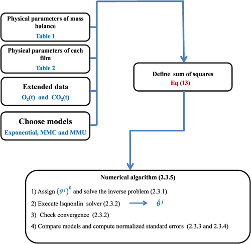
The numerical methodology, summarized in Figure 3, requires the physical parameters for the mass balance (given in Table 1), those specific for each film (given in Table 2), the extended data for $O_2$ and $C{O}_2$ concentrations, and choosing one of the three models, exponential, MMU and MMC. All these inputs are required to define the sum of squares given in Equation (13(13) $S({\mathit{\theta }}^j)={\displaystyle \sum _{i=1}^I\Vert {\mathbf{U}}_i^j-\mathbf{U}(i,{\mathit{\theta }}^j){\Vert }^2}$(13) ), which is the main input for the numerical optimization algorithm described in Section 2.3.2 that also requires the assignation of an initial parameters vector to compute an approximation of the nonlinear LSE.

3. Results

In this section, we present our numerical results concerning the $O_2$ and $C{O}_2$ concentration curves fitted to each dataset using the proposed models (exponential, MMU, and MMC). For each dataset (film j = 1, 2), the numerical results are shown in the following way:

• Initial guesses, nonlinear LSE, and normalized standard errors are shown in Tables 4, 6, and 8 for the exponential, MMU, and MMC models, respectively.

• Convergence metrics, initial and optimal values of the sum of squares, as well as fit performance are shown in Tables 5, 7, and  9 for the exponential, MMU, and MMC models, respectively.

• Fitted curves are depicted in Figure 4,  5, and 6 for the exponential, MMU, and MMC models, respectively.

• Effect of the uncertainty of data measurement and initial guess on parameter estimate are shown in Section 3.4.

Figure 4. Fitted curves for the exponential model. (a) Film PSF530 (b) Film PPCX.

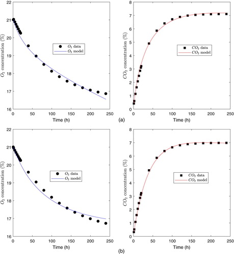
Figure 5. Fitted curves for the MMU model. (a) Film PSF530. (b) Film PPCX.

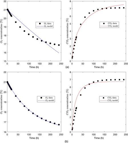
Figure 6. Fitted curves for the MMC model. (a) Film PSF530. (b) Film PPCX.

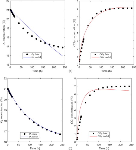
Table 4. Values for initial $({\mathit{\theta }}^j{)}^{(0)}$ and optimal ${\hat{\mathit{\theta }}}^j$ nonlinear LSE, and normalized standard errors ${\mathit{n}\mathit{s}\mathit{e}}^j$ for exponential model.

	Film PSF530			Film PPCX
Parameter	$({\mathit{\theta }}^1{)}^{(0)}$	${\hat{\mathit{\theta }}}^1$	${\mathit{n}\mathit{s}\mathit{e}}^1$	$({\mathit{\theta }}^2{)}^{(0)}$	${\hat{\mathit{\theta }}}^2$	${\mathit{n}\mathit{s}\mathit{e}}^2$
$\begin{array}{c}{A}_1\\ A_2\\ K\end{array}$	$\begin{array}{c}3.41\\ 5.5\\ 10.7\end{array}$	$\begin{array}{c}3.3301e-2\\ 1.0844e+3\\ 3.1839\end{array}$	$\begin{array}{c}1.7507\\ 1.3354\\ 4.3112e-1\end{array}$	$\begin{array}{c}6.82\\ 5.5\\ 10.7\end{array}$	$\begin{array}{c}2.3114e-2\\ 2.6974e+2\\ 3.2514\end{array}$	$\begin{array}{c}1.3579\\ 3.8445\\ 4.9309e-1\end{array}$

Table 5. Convergence metrics, initial $S(({\mathit{\theta }}^j{)}^{(0)})$ and optimal $S({\hat{\mathit{\theta }}}^j)$ values and fit performance for the exponential model.

Film	$||\mathbf{\nabla }S({\hat{\mathit{\theta }}}^j)|{|}_{\mathrm{\infty }}$	${\delta }_S^{(k)}$	k + 1	$S(({\mathit{\theta }}^j{)}^{(0)})$	$S({\hat{\mathit{\theta }}}^j)$	$({\tilde{\sigma }}^j{)}^2$	RMSE	$R^2$
PSF530	1.49e−13	1.53e−19	30	1.9435e−1	3.5920e−7	1.4967e−9	3.8931e−5	0.9914
PPCX	3.11e−13	4.33e−18	33	2.0853e−1	4.4406e−7	1.8502e−9	4.3286e−5	0.9892

Table 6. Values for initial $({\mathit{\theta }}^j{)}^{(0)}$ and optimal ${\hat{\mathit{\theta }}}^j$ nonlinear LSE, and normalized standard errors ${\mathit{n}\mathit{s}\mathit{e}}^j$ for the MMU model.

	Film PSF530			Film PPCX
Parameter	$({\mathit{\theta }}^1{)}^{(0)}$	${\hat{\mathit{\theta }}}^1$	${\mathit{n}\mathit{s}\mathit{e}}^1$	$({\mathit{\theta }}^2{)}^{(0)}$	${\hat{\mathit{\theta }}}^2$	${\mathbf{n}\mathbf{s}\mathbf{e}}^2$
$\begin{array}{c}{V}_{max}\\ K_m\\ K_u\end{array}$	$\begin{array}{c}1.3000e-3\\ 2.0000e-3\\ 1.3100e-1\end{array}$	$\begin{array}{c}8.2862e-5\\ 4.5195e-3\\ 1.5954e-5\end{array}$	$\begin{array}{c}9.7539e+1\\ 1.8543e+2\\ 9.7607e+1\end{array}$	$\begin{array}{c}1.3000e-3\\ 2.0000e-3\\ 1.3100e-1\end{array}$	$\begin{array}{c}7.5057e-5\\ 5.7782e-4\\ 3.5235e-5\end{array}$	$\begin{array}{c}3.4779e+1\\ 2.7269e+2\\ 3.4809e+1\end{array}$

Table 7. Convergence metrics, initial $S(({\mathit{\theta }}^j{)}^{(0)})$ and optimal $S({\hat{\mathit{\theta }}}^j)$ values and fit performance for the MMU model.

Film	$||\mathbf{\nabla }S({\hat{\mathit{\theta }}}^j)|{|}_{\mathrm{\infty }}$	${\delta }_S^{(k)}$	k + 1	$S(({\mathit{\theta }}^j{)}^{(0)})$	$S({\hat{\mathit{\theta }}}^j)$	$({\tilde{\sigma }}^j{)}^2$	RMSE	$R^2$
PSF530	4.8e−16	1.10e−20	75	7.7628	3.7158e−6	1.5483e−8	1.2521e−4	0.9107
PPCX	5.71e−7	4.66e−21	43	6.9119	2.5631e−6	1.0680e−8	1.0399e−4	0.9379

Table 8. Values for initial $({\mathit{\theta }}^j{)}^{(0)}$ and optimal ${\hat{\mathit{\theta }}}^j$ nonlinear LSE, and normalized standard errors ${\mathit{n}\mathit{s}\mathit{e}}^j$ for the MMC model.

	Film PSF530			Film PPCX
Parameter	$({\mathit{\theta }}^1{)}^{(0)}$	${\hat{\mathit{\theta }}}^1$	${\mathit{n}\mathit{s}\mathit{e}}^1$	$({\mathit{\theta }}^2{)}^{(0)}$	${\hat{\mathit{\theta }}}^2$	${\mathit{n}\mathit{s}\mathit{e}}^2$
$\begin{array}{c}{V}_{max}\\ K_m\\ K_c\end{array}$	$\begin{array}{c}1.3000e-2\\ 1.0000e-3\\ 1.3100e-1\end{array}$	$\begin{array}{c}8.2931e-5\\ 4.5195e-3\\ 1.7791e-5\end{array}$	$\begin{array}{c}5.0071e+1\\ 2.6455e+2\\ 2.1470e+2\end{array}$	$\begin{array}{c}1.3000e-2\\ 1.0000e-3\\ 1.3100e-1\end{array}$	$\begin{array}{c}7.9734e-5\\ 9.2464e-4\\ 7.7281e-6\end{array}$	$\begin{array}{c}9.0115e+1\\ 1.7132e+2\\ 8.1337e+1\end{array}$

Table 9. Convergence metrics, initial $S(({\mathit{\theta }}^j{)}^{(0)})$ and optimal $S({\hat{\mathit{\theta }}}^j)$ values and fit performance for the MMC model.

Film	$||\mathbf{\nabla }S({\hat{\mathit{\theta }}}^j)|{|}_{\mathrm{\infty }}$	${\delta }_S^{(k)}$	k + 1	$S(({\mathit{\theta }}^j{)}^{(0)})$	$S({\hat{\mathit{\theta }}}^j)$	$({\tilde{\sigma }}^j{)}^2$	RMSE	$R^2$
PSF530	7.77e−16	2.46e−20	29	7.9580	3.1769e−6	1.3237e−8	1.1578e−4	0.9237
PPCX	1.13e−7	1.02e−20	76	6.1954	4.3293e−6	1.8039e−8	1.3516e−4	0.8951

We recall that the initial guesses and nonlinear LSE were designated by $({\mathit{\theta }}^j{)}^{(0)}$ and ${\hat{\mathit{\theta }}}^j$, respectively, while the normalized standard errors were denoted by ${\mathbf{n}\mathbf{s}\mathbf{e}}^j$ and defined in Equation (24(24) ${\mathbf{s}\mathbf{e}}_l^j=\sqrt{{\left(Co{v}^j\right)}_{l,l}},{\mathbf{n}\mathbf{s}\mathbf{e}}_l^j=100\cdot \frac{{\mathit{s}\mathit{e}}_l^j}{{\hat{\mathit{\theta }}}_l^j},l=1,2,3;j=1,2$(24) ). The initial guess $({\mathit{\theta }}^j{)}^{(0)}$ was computed as summarized in Step (1), while the nonlinear LSE ${\hat{\mathit{\theta }}}^j$ was computed as summarized in Step (2) of the previous section. The convergence metrics ${\delta }_{\mathit{\theta }}^{(k)}$, ${\delta }_S^{(k)}$, and $\Vert \mathrm{\nabla }S({\hat{\mathit{\theta }}}^j){\Vert }_{\mathrm{\infty }}$ defined in Equations (15(15) ${\delta }_{\mathit{\theta }}^{(k)}=\Vert {\mathit{\theta }}^{(k+1)}-{\mathit{\theta }}^{(k)}\Vert$(15) ), (16(16) ${\delta }_S^{(k)}=\frac{|S({\mathit{\theta }}^{(k)})-S({\mathit{\theta }}^{(k+1)})|}{1+|S({\mathit{\theta }}^{(k)})|}$(16) ), and (18(18) $\Vert \mathbf{\nabla }S({\hat{\mathit{\theta }}}^j){\Vert }_{\mathrm{\infty }}=\underset{\ell =1,2,3}{max}|\frac{\mathrm{\partial }S}{\mathrm{\partial }{\mathit{\theta }}_{\ell }^j}({\hat{\mathit{\theta }}}^j)|$(18) ), respectively, are the outputs arguments of the lsqnonlin Matlab${}^{\circledR }$ solver. We note that the number of iterations that are necessary to converge corresponds to k + 1 in the nomenclature of Matlab${}^{\circledR }$ (k starts at 0). The sum of squares $S({\mathit{\theta }}^j)$ was defined by Equation (13(13) $S({\mathit{\theta }}^j)={\displaystyle \sum _{i=1}^I\Vert {\mathbf{U}}_i^j-\mathbf{U}(i,{\mathit{\theta }}^j){\Vert }^2}$(13) ), while fit performance was quantified by the goodness-of-fit criteria $({\tilde{\sigma }}^2{)}^j$, ${\hat{\sigma }}^j$ and $R^{2,j}$ defined in Equations (19(19) $\begin{array}{rl}({\tilde{\sigma }}^j{)}^2& =\frac{S({\hat{\mathit{\theta }}}^j)}{I}\end{array}$(19) )–(21(21) $\begin{array}{rl}{R}^{2,j}& =1-\frac{S({\hat{\mathit{\theta }}}^j)}{\sum _{i=1}^I[{((n_{O_2}{)}_i^j-{\overline{n_{O_2}}}^j)}^2+{((n_{C{O}_2}{)}_i^j-{\overline{n_{C{O}_2}}}^j)}^2]}\end{array}$(21) ).

3.1. Results for the exponential model

Table 4 shows the initial parameter estimate $({\mathit{\theta }}^j{)}^{(0)}=((A_1^j{)}^{(0)},(A_2^j{)}^{(0)},(K^j{)}^{(0)})$, the nonlinear LSE ${\hat{\mathit{\theta }}}^j=({\hat{A}}_1^j,{\hat{A}}_2^j,{\hat{K}}^j)$, and the normalized standard errors ${\mathbf{n}\mathbf{s}\mathbf{e}}^j$ computed for each dataset j = 1, 2.

In addition, Table 5 shows the convergence metrics, initial and optimal values of the sum of squares, as well as fit performance for each dataset j = 1, 2.

Finally, Figure 4 depicts the fit of the exponential model to the datasets j = 1, 2. Few data points are shown to differentiate them from the theoretical curves.

3.2. Results for the MMU model

In the present study, besides the options chosen for the lsqnonlin solver, we set as the upper bound for the parameter $K_m$ the maximum experimental value for the $O_2$ concentration because $K_m$ represents the half of the latter.

Table 6 shows the initial parameter estimate $({\mathit{\theta }}^j{)}^{(0)}=((V_{max}^j{)}^{(0)},(K_m^j{)}^{(0)},(K_u^j{)}^{(0)})$, the nonlinear LSE ${\hat{\mathit{\theta }}}^j=({\hat{V}}_{max}^j,{\hat{K}}_m^j,{\hat{K}}_u^j)$, and the normalized standard errors ${\mathbf{n}\mathbf{s}\mathbf{e}}^j$ computed for each dataset j = 1, 2.

In addition, Table 7 shows the convergence metrics, initial and optimal values of the sum of squares, as well as fit performance.

Finally, Figure 5 depicts the fit of the MMU model to the datasets j = 1, 2. Few data points are shown to differentiate them from the theoretical curves.

3.3. Results for the MMC model

As for the MMU model, we also set as the upper bound for the parameter $K_m$ the maximum experimental value for the $O_2$ concentration.

Table 8 shows the initial parameter estimate $({\mathit{\theta }}^j{)}^{(0)}=((V_{max}^j{)}^{(0)},(K_m^j{)}^{(0)},(K_c^j{)}^{(0)})$, the nonlinear LSE ${\hat{\mathit{\theta }}}^j=({\hat{V}}_{max}^j,{\hat{K}}_m^j,{\hat{K}}_c^j)$, and the normalized standard errors ${\mathbf{n}\mathbf{s}\mathbf{e}}^j$ computed for each dataset j = 1, 2.

In addition, Table 9 shows the convergence metrics, initial and optimal values, as well as fit performance for the MMC model.

Finally, Figure 6 depicts the fit of the MMC model to the datasets j = 1, 2. Few data points are shown to differentiate them from the theoretical curves.

3.4. Effect of the uncertainty of data measurement and initial guess on parameter estimate

In this subsection, we quantify the effect of the uncertainty of data measurement and initial guess on parameter estimate. To make that, we considered two simulated datasets constructed using the exponential model and the nonlinear LSE computed for the two film types. More precisely, we have taken ${\hat{\mathit{\theta }}}^j$ for j = 1, 2 from Table 4 and computed the concentrations curves for $O_2$ and $C{O}_2$ using the exponential model evaluated at these two nonlinear LSE, and we used them to generate exact data. Then, we perturbed these datasets by adding Gaussian noise to each of them to simulate the measurement errors on data. From these perturbed data, we computed parameter estimates using as initial guesses the nonlinear LSE that generated the exact datasets for the optimization algorithm, thereby quantifying the effect of uncertainty of data measurement on parameter estimate.

Exact data were perturbed by adding Gaussian noise ${\mathit{\epsilon }}^j\stackrel{\mathrm{i}.\mathrm{i}.\mathrm{d}.}{\sim }\mathcal{N}(0,{\mathbf{\Sigma }}^2)$ to the exact data, where we choose $\mathbf{\Sigma }=(1.3e-4,4.5e-5)$ to verify the condition $\mathbf{\Sigma }/max\{\mathbf{U}(i,{\hat{\mathit{\theta }}}^j)|i=1,\dots ,I\}<3.0e-2$ for both films types, thereby to not obtain negative perturbed data.

Figure 7 depicts the perturbed and exact data for both film types, where few data points are shown to differentiate them.

Figure 7. Simulated data obtained from the exponential model. (a) Film PSF530. (b) Film PPCX.

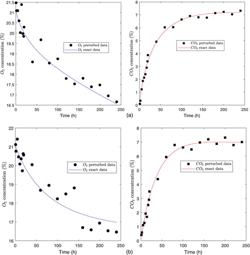
Table 10 shows the relative errors for parameter estimate and variables of the exponential model, as well as the convergence metrics computed by the optimization solver.

Table 10. Relative errors and convergence metrics for perturbed data with Gaussian noise.

Film	$E_{{\mathit{\theta }}^{j,p}}^R$	$E_{n_{O_2}^j}^R$	$E_{n_{C{O}_2}^j}^R$	$||\mathbf{\nabla }S({\hat{\mathit{\theta }}}^{j,p})|{|}_{\mathrm{\infty }}$	${\delta }_{S,p}^{(k)}$	k + 1	$S({\hat{\mathit{\theta }}}^{j,p})$	$S({\hat{\mathit{\theta }}}^j)$
PSF530	1.2366e−1	1.0279e−1	9.1993e−2	1.32e−13	1.86e−20	6	4.7668e−6	6.1732e−6
PPCX	9.7632e−2	8.0255e−2	9.6583e−2	9.93e−14	3.05e−20	6	4.0784e−6	4.1311e−6

Relative errors were computed as $E_{{\mathit{\theta }}^{j,p}}^R=\Vert {\hat{\mathit{\theta }}}^j-{\hat{\mathit{\theta }}}^{j,p}{\Vert }_{\mathrm{\infty }}/\Vert {\hat{\mathit{\theta }}}^j{\Vert }_{\mathrm{\infty }}$, where ${\hat{\mathit{\theta }}}^{j,p}$ stands for the perturbed nonlinear LSE, i.e. the nonlinear LSE computed for fitting the exponential model to the perturbed datasets for each j = 1, 2, and the relative errors $E_{n_{O_2}^j}^R$, $E_{n_{C{O}_2}^j}^R$ were similarly computed.

Convergence metrics $\Vert \mathbf{\nabla }S({\hat{\mathit{\theta }}}^{j,p}){\Vert }_{\mathrm{\infty }}$, ${\delta }_{S,p}^{(k)}$, $S({\hat{\mathit{\theta }}}^{j,p})$ correspond to the first-order optimality measure defined in (18(18) $\Vert \mathbf{\nabla }S({\hat{\mathit{\theta }}}^j){\Vert }_{\mathrm{\infty }}=\underset{\ell =1,2,3}{max}|\frac{\mathrm{\partial }S}{\mathrm{\partial }{\mathit{\theta }}_{\ell }^j}({\hat{\mathit{\theta }}}^j)|$(18) ), the relative change in the sum of squares defined in (16(16) ${\delta }_S^{(k)}=\frac{|S({\mathit{\theta }}^{(k)})-S({\mathit{\theta }}^{(k+1)})|}{1+|S({\mathit{\theta }}^{(k)})|}$(16) ), the optimal value of the objective function, respectively, where the three previous metrics are evaluated at the perturbed nonlinear LSE ${\hat{\mathit{\theta }}}^{j,p}$. Also, k + 1 and $S({\hat{\mathit{\theta }}}^j)$ correspond to the number of iterations and the initial value of the objective function, respectively.

Finally, to quantify the effect of the uncertainty of initial guess on parameter estimate, we have taken the initial guesses $({\mathit{\theta }}^j{)}^{(0)}$ considered for the exponential model in Table 4, and we perturbed them by adding Gaussian noise ${\mathit{\epsilon }}^j\stackrel{\mathrm{i}.\mathrm{i}.\mathrm{d}.}{\sim }\mathcal{N}(0,{\mathbf{\Sigma }}^2)$, choosing $\mathbf{\Sigma }=\Vert ({\mathit{\theta }}^j{)}^{(0)}{\Vert }_{\mathrm{\infty }}\cdot (1,1,1)$ (all the components of $\mathbf{\Sigma }$ equal to the maximum initial parameters vector value), taking care that all the perturbed initial parameters vector components, $({\mathit{\theta }}^{j,p}{)}^{(0)}$, be positive for the two films j = 1, 2.

Table 11 shows the relative errors for initial and optimal parameter estimates for the exponential model, as well as the convergence metrics computed by the optimization solver. All these quantities were similarly computed as we made for Table 10.

Table 11. Relative errors and convergence metrics for perturbed initial parameters with Gaussian noise.

Film	$E_{({\mathit{\theta }}^{j,p}{)}^{(0)}}^R$	$E_{{\hat{\mathit{\theta }}}^{j,p}}^R$	$||\mathbf{\nabla }S({\hat{\mathit{\theta }}}^{j,p})|{|}_{\mathrm{\infty }}$	${\delta }_{S,p}^{(k)}$	k + 1	$S({\hat{\mathit{\theta }}}^{j,p})$	$S(({\mathit{\theta }}^{j,p}{)}^{(0)})$
PSF530	2.7304	5.1672e−8	2.89e−13	2.27e−18	19	3.5920e−7	2.8542
PPCX	1.2413e + 2	1.5921e−8	3.07e−14	3.69e−19	66	4.4406e−7	1.4472e−2

4. Discussion

When we analyse the convergence metrics of the numerical method in Table 5 (first three columns), we observe that they are very successful for the exponential model. We conclude that our method approximately converges, i.e. the nonlinear LSE ${\hat{\mathit{\theta }}}^j$ is very close to the actual minimum for each dataset j = 1, 2. On the other hand, fit performance is very good, which is reflected by the fact that the variance and RMSE explained by the exponential model are rather low, while the coefficient of determination is very close to 1. In addition, from the data in Table 4, we can observe that the normalized standard errors $\mathit{n}\mathit{s}\mathit{e}$ are rather low (less than 4%), which provides a very accurate parameter estimation. This is in accordance with the fitted curves, shown in Figure 4, that are very close to the data for the exponential model. Figure 4 also shows that the $C{O}_2$ concentration reaches equilibrium before the $O_2$ concentration, which is determined by the distribution of data. The time to reach equilibrium also depends on the permeability ratio. In fact, $O_2$ permeability for Film PSF530 is an order of magnitude less than $C{O}_2$ permeability, and $O_2$ decays faster than in Film PPCX, for which permeability for both, $O_2$ and $C{O}_2$, have the same order of magnitude.

In the case of MMU model, from the data in Table 7 we can observe that convergence metrics are relatively successful. We conclude that our method approximately converges, i.e. the nonlinear LSE ${\hat{\mathit{\theta }}}^j$ is relatively close to the actual minimum for each dataset j = 1, 2. However, according to data shown in Table 6, normalized standard errors $\mathit{n}\mathit{s}\mathit{e}$ are rather high (greater than 34%), which provides an inaccurate parameter estimation for the MMU model compared to the exponential model. This is in accordance with the fitted curves, shown in Figure 5, which confirms that the fit is relatively inaccurate for the MMU model. On the other hand, Figure 5(a) shows that the fit to data for Film PSF530 is more inaccurate, which is numerically confirmed by the fact that the variance and RMSE are higher, while the coefficient of determination is lower than for Film PPCX (Table 7). This is also confirmed by higher normalized standard errors for components 1 and 3 of the nonlinear LSE for film PSF530 compared to Film PPCX (${\mathit{n}\mathit{s}\mathit{e}}^1$ and ${\mathit{n}\mathit{s}\mathit{e}}^2$ in Table 6), which indicates that parameters $V_{\max }$ and $K_u$ are more inaccurately estimated for Film PSF530.

A similar discussion as for MMU model also applies for the MMC model. In fact, similar convergence metrics for the MMC model are shown in Table 9. We can, therefore, conclude that our method approximately converges, i.e. the nonlinear LSE ${\hat{\mathit{\theta }}}^j$ is relatively close to the actual minimum for each dataset j = 1, 2. On the other hand, similar fit performance is observed for both models, because values for the goodness-of-fit criteria are very similar. On the other hand, Table 8 indicates that normalized standard errors $\mathit{n}\mathit{s}\mathit{e}$ are rather high (greater than 50 %), which implies an inaccurate parameter estimation for the MMC model. If we analyse Figure 6, a better fit is observed for Film PSF530 than for Film PPCX. On the other hand, we can observe that its fit to data is better for the PPCX film in the case of the $O_2$. In contrast, the fit to data is better for film PSF530 film in the case of the $C{O}_2$.

When quantifying the effect of data measurement errors for the exponential model, we found from Table 10 that the relative error for parameter estimate is of the same order of magnitude that for $O_2$ and $C{O}_2$ concentrations (for both films types), and convergence metrics for perturbed data are successful, which implies the robustness of the proposed methodology.

Finally, when quantifying the uncertainty of initial guess on parameter estimate, we found from Table 11 that the computed parameter estimates were almost the same, which implies that our method is stable. It is worth noting that the issue of the suitable choice of the initial guess is crucial when no a priori information is available on the actual values of the model parameters, or when having the observation of only a partial combination of the model variables [11].

5. Summary and conclusions

In this work, we have described in a clear way and successfully implemented a modern and efficient parameter estimation methodology which we believe is useful to apply for all the MAP technology-related community. We have illustrated our methodology to carry out parameter estimation for two datasets corresponding to two film types. The numerical results obtained for the three models proposed show that the exponential one is that best fits for both datasets, which means that the respiration rate exponentially decays when the $C{O}_2$ concentration increases. It is worth noting that the Michaelis–Menten models are not as appropriate as the exponential model since the last has the best convergence metrics, as well as the best normalized standard errors. On the other hand, the type of film is a fundamental variable in MAP systems. In this sense, results for the exponential model are similar for both film types, whereas results for the Michaelis–Menten models are different. On the other hand, the methodology proposed is robust since we can compute suitable parameter estimate when data have uncertainties in their measurement, as well as when appropriate initial guesses are not known a priori, i.e. no a priori information is available on the actual values of the model parameters.

We expect that our methodology serves as a tool for assessing MAP technology design since it is relatively easy to apply, and the only requirement is a conventional PC endowed with Matlab${}^{\circledR }$ software. However, it is worth noting that this is made to avoid implementing the optimization algorithm, and in this sense, any software having a suitable predefined optimization toolbox may serve to our purpose.

Disclosure statement

The authors declare no conflict of interest.

Additional information

Funding

The work of P.C. was supported by PIA-CONICYT grant FB-01, by grants DIUBB-GI 171709/VC and DIUBB 193409 3/R. The work of G.B. and L.S. were supported by CORFO, project Innova Biobio 16IIP65192 and Fondef ID16I10206.

References

- Mangaraj S, Goswami TK. Modeling of respiration rate of litchi fruit under aerobic conditions. Food Bioproc Tech. 2008 Oct;4(2):272–281. doi: 10.1007/s11947-008-0145-z
- Makino Y. Oxygen consumption by fruits and vegetables. Food Sci Technol Res. 2013 Sept;19:523–529. doi: 10.3136/fstr.19.523
- Heydari A, Shayesteh K, Eghbalifam N, et al. Studies on the respiration rate of banana fruit based on enzyme kinetics. Int J Agric Biol. 2010;12(1):145–149.
- Yahia EM. Introduction. In: Yahia EM, editor. Modified and controlled atmospheres for the storage, transportation, and packaging of horticultural commodities. Chapter 1. Boca Raton: CRC press; 2009. p. 1–16.
- Del Nobile M, Sinigaglia M, Conte A, et al. Influence of postharvest treatments and film permeability on quality decay kinetics of minimally processed grapes. Postharvest Biol Technol. 2008;47(3):389–396. Available from: http://www.sciencedirect.com/science/article/pii/S0925521407002335 doi: 10.1016/j.postharvbio.2007.07.004
- Henig YS, Gilbert SG. Computer analysis of the variables affecting respiration and quality of produce packaged in polymeric films. J Food Sci. 1975;40(5):1033–1035. Available from: https://onlinelibrary.wiley.com/doi/abs/10.1111/j.1365-2621.1975.tb02261.x
- Fonseca SC, Oliveira FA, Brecht JK. Modelling respiration rate of fresh fruits and vegetables for modified atmosphere packages: a review. J Food Eng. 2002;52(2):99–119. Available from: http://www.sciencedirect.com/science/article/pii/S0260877401001066 doi: 10.1016/S0260-8774(01)00106-6
- Belay ZA, Caleb OJ, Opara UL. Modelling approaches for designing and evaluating the performance of modified atmosphere packaging (map) systems for fresh produce: a review. Food Packag Shelf Life. 2016;10:1–15. Available from: http://www.sciencedirect.com/science/article/pii/S2214289416300813 doi: 10.1016/j.fpsl.2016.08.001
- Del Nobile M, Baiano A, Benedetto A, et al. Respiration rate of minimally processed lettuce as affected by packaging. J Food Eng. 2006;74(1):60–69. Available from: http://www.sciencedirect.com/science/article/pii/S0260877405001068 doi: 10.1016/j.jfoodeng.2005.02.013
- Guillard V, Guillaume C, Destercke S. Parameter uncertainties and error propagation in modified atmosphere packaging modelling. Postharvest Biol Technol. 2012;67:154–166. Available from: http://www.sciencedirect.com/science/article/pii/S0925521411003140 doi: 10.1016/j.postharvbio.2011.12.014
- Cumsille P, Godoy M, Gerdtzen ZP. Parameter estimation and mathematical modeling for the quantitative description of therapy failure due to drug resistance in gastrointestinal stromal tumor metastasis to the liver. PLoS One. 2019 May;14(5):1–27. doi: 10.1371/journal.pone.0217332
- Cumsille P, Coronel A, Conca C, et al. Proposal of a hybrid approach for tumor progression and tumor-induced angiogenesis. Theor Biol Med Model. 2015;12(1):13. doi: 10.1186/s12976-015-0009-y
- Charles F, Guillaume C, Gontard N. Effect of passive and active modified atmosphere packaging on quality changes of fresh endives. Postharvest Biol Technol. 2008;48(1):22–29. Available from: http://www.sciencedirect.com/science/article/pii/S0925521407003407 doi: 10.1016/j.postharvbio.2007.09.026
- Yunus CA, Afshin GJ. Heat and mass transfer: fundamentals and applications. Chapter 14. New York: McGraw-Hill Education; 2015. p. 835–906.
- Coleman TF, Li Y. An interior trust region approach for nonlinear minimization subject to bounds. SIAM J Optim. 1996;6(2):418–445. doi: 10.1137/0806023
- MathWorks. Nonlinear least squares (curve fitting) [internet]; 2017. Available from: https://www.mathworks.com/help/optim/nonlinear-least-squares-curve-fitting.html
- Shampine LF, Reichelt MW. The matlab ode suite. SIAM J Sci Comput. 1997;18(1):1–22. doi: 10.1137/S1064827594276424
- Banks HT, Davidian M, Samuels JR. An inverse problem statistical methodology summary. In: Chowell G, Hyman JM, Bettencourt LMA, et al., editors. Mathematical and statistical estimation approaches in epidemiology. Dordrecht: Springer; 2009. p. 249–302.
- Greene WH. Econometric analysis. New Jersey (NY): Pearson; 2012.
- Banks H, Dediu S, Ernstberger S. Sensitivity functions and their uses in inverse problems. J Inverse Ill-Pose P. 2008;15(7):683–708.