Analytic series solutions of 2D forward and backward heat conduction problems in rectangles and a new regularization

Abstract

In the paper, we solve a non-homogeneous heat conduction equation with non-homogeneous boundary conditions in a 2D rectangle. First, we derive the domain/boundary integral equations for both the forward and backward heat conduction problems. Then, by using the technique of homogenization, inserting the adjoint Trefftz test functions into the derived integral equations and expanding the solutions in terms of eigenfunctions, we can obtain the expansion coefficients in closed form. Hence, the analytic series solutions of forward heat conduction problems (FHCPs) and backward heat conduction problems (BHCPs) are available. For the FHCPs, only a few terms in the series render very high-order accurate solutions at any time, with errors of the order ${10}^{-10}$. For the BHCPs, we require to modify the closed-form series solutions via a new spring-damping regularization technique. Numerical tests for the BHCPs in a large space-time domain reveal that the present analytic series solution is very accurate to recover the initial temperature with an error of the order ${10}^{-10}$, although the measured final time temperature is very small when $t_f$ is large up to 100 and is even polluted by a large relative noise up to the level $20\mathrm{\%}$.

Keywords:

• 2D heat conduction equation
• domain/boundary integral equation
• Adjoint Trefftz test functions
• backward heat conduction problem
• analytic series solution
• spring-damping regularization

2010 Mathematics Subject Classifications:

• 35K05
• 35K55
• 45L05
• 65M32
• 65R20

1. Introduction

Let us consider a 2D heat conduction equation: (1) $\begin{array}{rl}& u_t(x,y,t)=u_{xx}(x,y,t)+u_{yy}(x,y,t)+S(x,y,t),\\ & (x,y,t)\in \mathrm{\Omega }:=\{0<x<a,0<y<b,0<t\le t_f\},\end{array}$(1) (2) $\begin{array}{rl}& u(0,y,t)=h_1(y,t),\\ & u(a,y,t)=h_2(y,t),\\ & u(x,0,t)=h_3(x,t),\\ & u(x,b,t)=h_4(x,t),\end{array}$(2) where the subscripts x, y and t denote the partial differentials with respect to x, y and t, respectively. We give the heat source term $S(x,y,t)$ and the following initial condition: (3) $u(x,y,0)=f(x,y),$(3) for the forward heat conduction problem (FHCP), whose analytic solution is in general not available. In the past few decades, many accurate and efficient numerical methods for the FHCPs have been developed, such as the finite element method, the finite volume method, the boundary element method and the meshless method [1–9]. Those numerical methods take different techniques to enhance the accuracy and stability of numerical solutions; however, it is hard to avoid the numerical error accumulated and propagated in the time direction. In order to overcome these difficulties, we will propose a highly accurate closed-form series solution of the 2D FHCP, which can avoid the time integration error and the propagation of error.

On the other hand, we may sometimes require to seek an unknown initial temperature of an object in a practical heat conduction problem. For this purpose, we can measure the present temperature as a final time condition (4) $u(x,y,t_f)=g(x,y).$(4) Thus, we encounter a backward heat conduction problem (BHCP) to recover the initial condition (3(3) $u(x,y,0)=f(x,y),$(3) ) and then we may need to solve an FHCP with the recovered initial condition to obtain the solution $u(x,y,t)$ in the whole space-time domain Ω.

The earlier works for the BHCP were carried by Cannon [10–12]. In order to solve the BHCPs, there were a lot of progresses, including the boundary element method [13], the iterative boundary element method [14,15], the Tikhonov regularization technique [16,17], the operator-splitting method [18], the lattice-free high-order finite difference method [19], the method of fundamental solutions [20,21], the third-order mixed-derivative regularization technique [22], the Fourier regularization method [23], the three-spectral regularization method [24], the radial-basis functions method [25], the quasi-reversibility method [26–28], and the backward fictitious time integration method [29].

The first author and his co-workers have developed many methods to solve the BHCPs, namely, the group preserving scheme [30], the backward group preserving scheme [31], Lie-group shooting method together with the quasi-boundary regularization [28], the Fredholm integral equation method [32,33], the Lie-group shooting method in the time direction [34], the Lie-group shooting method in the spatial direction [35], the fictitious time integration method [36], a self-adaptive Lie-group shooting method [37], the method of fundamental solutions with conditioning by a new post-conditioner [38], a two-stage group preserving scheme [39], the $GL(n,\mathbb{R})$ shooting method [40], and a Lie-group differential-algebraic equations method [41]. Recently, Liu [42] has solved the BHCP without resorting on the final time condition and the over-specified boundary conditions, and Liu [43] has solved the high-dimensional BHCP by using the multiple/scale/direction polynomial Trefftz method.

The numerical approaches of the BHCPs with regularization techniques have been adopted widely, like the Tikhonov regularization, the maximum entropy principle, and the truncated singular value decomposition [16,17], the conjugate gradient method with an adjoint equation [44], and the method of fundamental solutions with the standard Tikhonov regularization technique [45]. In the current paper, we propose a new and effective regularization technique based on the analytic closed-form series solution, which is very accurate even the 2D BHCP is with a long time span. There are many applications of the BHCP, for example, the detection of initial pollution profile in the river [46].

The analytic solutions of both the FHCPs and the BHCPs in terms of a homogenization function and the closed-form series are proposed for the first time. The remained portions of the paper are arranged as follows. In Section 2, we derive a domain/boundary integral equation for the 2D heat conduction equation of a rectangular plate. In Section 3, a stable adjoint Trefftz test function is derived for the 2D FHCP, resulting to a simplified integral equation, and then a homogenization function is derived, such that we can obtain a closed-form series solution. For the 2D BHCP, by using the same stable adjoint Trefftz test function, we can derive a simplified integral equation, and then another homogenization function in Section 4, such that we can obtain a closed-form series solution, where a new regularization technique based on the idea in the spring-damping behaviour of vibration equation is introduced. While the numerical tests of the FHCP are given in Section 5, those for the BHCP are given in Section 6. Finally, we draw some conclusions in Section 7.

2. Domain/boundary integral equation method

We consider the 2D heat operator and its adjoint operator (5) $\begin{array}{rl}\mathcal{H}(u)& =\frac{\mathrm{\partial }u}{\mathrm{\partial }t}-\frac{{\mathrm{\partial }}^{2}u}{\mathrm{\partial }{x}^2}-\frac{{\mathrm{\partial }}^{2}u}{\mathrm{\partial }{y}^2},\end{array}$(5) (6) $\begin{array}{rl}{\mathcal{H}}^{\ast }(v)& =-\frac{\mathrm{\partial }v}{\mathrm{\partial }t}-\frac{{\mathrm{\partial }}^{2}v}{\mathrm{\partial }{x}^2}-\frac{{\mathrm{\partial }}^{2}v}{\mathrm{\partial }{y}^2}.\end{array}$(6)

Theorem 2.1

Let Ω be a bounded region in the space $(x,y,t)$ with $(x,y,t)\in \mathrm{\Omega }:=\{0<x<a,0<y<b,0<t\le t_f\}$. Let $u(x,y,t)$ and $v(x,y,t)$ be functions that are differentiable in Ω and continuous on $\overline{\mathrm{\Omega }}$. Then, (7) $\begin{array}{rl}{\iiint }_{\mathrm{\Omega }}[v\mathcal{H}(u)-u{\mathcal{H}}^{\ast }(v)]\mathrm{d}x\mathrm{d}y\mathrm{d}t& ={\oint }_{{\mathrm{\Gamma }}_1}uv\mathrm{d}x\mathrm{d}y+{\oint }_{{\mathrm{\Gamma }}_2}[u{v}_x-v{u}_x]\mathrm{d}y\mathrm{d}t\\ & +{\oint }_{{\mathrm{\Gamma }}_3}[v{u}_y-u{v}_y]\mathrm{d}x\mathrm{d}t.\end{array}$(7)

Proof.

Let $\begin{array}{rl}{\mathrm{\Gamma }}_1& =\{0\le x\le a,0\le y\le b,t=0\}\cup \{0\le x\le a,0\le y\le b,t=t_f\},\\ {\mathrm{\Gamma }}_2& =\{0\le y\le b,0\le t\le t_f,x=0\}\cup \{0\le y\le b,0\le t\le t_f,x=a\},\\ {\mathrm{\Gamma }}_3& =\{0\le x\le a,0\le t\le t_g,y=0\}\cup \{0\le x\le a,0\le t\le t_g,y=b\}.\end{array}$ The following operations are available $\begin{array}{rl}{\iiint }_{\mathrm{\Omega }}{u}_{t}v\mathrm{d}x\mathrm{d}y\mathrm{d}t& ={\iiint }_{\mathrm{\Omega }}{u}_{t}v\mathrm{d}t\mathrm{d}x\mathrm{d}y\\ & ={\oint }_{{\mathrm{\Gamma }}_1}uv\mathrm{d}x\mathrm{d}y-{\iiint }_{\mathrm{\Omega }}u{v}_t\mathrm{d}x\mathrm{d}y\mathrm{d}t,\\ {\iiint }_{\mathrm{\Omega }}{u}_{xx}v\mathrm{d}x\mathrm{d}y\mathrm{d}t& ={\oint }_{{\mathrm{\Gamma }}_2}{u}_{x}v\mathrm{d}y\mathrm{d}t-{\iiint }_{\mathrm{\Omega }}{u}_x{v}_x\mathrm{d}x\mathrm{d}y\mathrm{d}t\\ & ={\oint }_{{\mathrm{\Gamma }}_2}{u}_{x}v\mathrm{d}y\mathrm{d}t-{\oint }_{{\mathrm{\Gamma }}_2}u{v}_x\mathrm{d}y\mathrm{d}t+{\iiint }_{\mathrm{\Omega }}u{v}_{xx}\mathrm{d}x\mathrm{d}y\mathrm{d}t,\\ {\iiint }_{\mathrm{\Omega }}{u}_{yy}v\mathrm{d}x\mathrm{d}y\mathrm{d}t& =-{\iiint }_{\mathrm{\Omega }}{u}_{yy}v\mathrm{d}y\mathrm{d}x\mathrm{d}t\\ & =-{\oint }_{{\mathrm{\Gamma }}_3}{u}_{y}v\mathrm{d}x\mathrm{d}t+{\iiint }_{\mathrm{\Omega }}{u}_y{v}_y\mathrm{d}y\mathrm{d}x\mathrm{d}t\\ & =-{\oint }_{{\mathrm{\Gamma }}_3}{u}_{y}v\mathrm{d}x\mathrm{d}t+{\oint }_{{\mathrm{\Gamma }}_3}u{v}_y\mathrm{d}x\mathrm{d}t-{\iiint }_{\mathrm{\Omega }}u{v}_{yy}\mathrm{d}y\mathrm{d}x\mathrm{d}t\\ & =-{\oint }_{{\mathrm{\Gamma }}_3}{u}_{y}v\mathrm{d}x\mathrm{d}t+{\oint }_{{\mathrm{\Gamma }}_3}u{v}_y\mathrm{d}x\mathrm{d}t+{\iiint }_{\mathrm{\Omega }}u{v}_{yy}\mathrm{d}x\mathrm{d}y\mathrm{d}t.\end{array}$ Then, we can obtain (8) $\begin{array}{rl}{\iiint }_{\mathrm{\Omega }}\mathcal{H}(u)v\mathrm{d}x\mathrm{d}y\mathrm{d}t& ={\iiint }_{\mathrm{\Omega }}u(-v_t-v_{xx}-v_{yy})\mathrm{d}x\mathrm{d}y\mathrm{d}t\\ & +{\oint }_{{\mathrm{\Gamma }}_1}uv\mathrm{d}x\mathrm{d}y+{\oint }_{{\mathrm{\Gamma }}_2}[u{v}_x-v{u}_x]\mathrm{d}y\mathrm{d}t\\ & +{\oint }_{{\mathrm{\Gamma }}_3}[v{u}_y-u{v}_y]\mathrm{d}x\mathrm{d}t.\end{array}$(8) By Equation (6(6) $\begin{array}{rl}{\mathcal{H}}^{\ast }(v)& =-\frac{\mathrm{\partial }v}{\mathrm{\partial }t}-\frac{{\mathrm{\partial }}^{2}v}{\mathrm{\partial }{x}^2}-\frac{{\mathrm{\partial }}^{2}v}{\mathrm{\partial }{y}^2}.\end{array}$(6) ), we can prove Equation (7(7) $\begin{array}{rl}{\iiint }_{\mathrm{\Omega }}[v\mathcal{H}(u)-u{\mathcal{H}}^{\ast }(v)]\mathrm{d}x\mathrm{d}y\mathrm{d}t& ={\oint }_{{\mathrm{\Gamma }}_1}uv\mathrm{d}x\mathrm{d}y+{\oint }_{{\mathrm{\Gamma }}_2}[u{v}_x-v{u}_x]\mathrm{d}y\mathrm{d}t\\ & +{\oint }_{{\mathrm{\Gamma }}_3}[v{u}_y-u{v}_y]\mathrm{d}x\mathrm{d}t.\end{array}$(7) ).

3. An analytic series solution of the FHCP

After inserting Equations (1(1) $\begin{array}{rl}& u_t(x,y,t)=u_{xx}(x,y,t)+u_{yy}(x,y,t)+S(x,y,t),\\ & (x,y,t)\in \mathrm{\Omega }:=\{0<x<a,0<y<b,0<t\le t_f\},\end{array}$(1) )–(3(3) $u(x,y,0)=f(x,y),$(3) ) into Equation (7(7) $\begin{array}{rl}{\iiint }_{\mathrm{\Omega }}[v\mathcal{H}(u)-u{\mathcal{H}}^{\ast }(v)]\mathrm{d}x\mathrm{d}y\mathrm{d}t& ={\oint }_{{\mathrm{\Gamma }}_1}uv\mathrm{d}x\mathrm{d}y+{\oint }_{{\mathrm{\Gamma }}_2}[u{v}_x-v{u}_x]\mathrm{d}y\mathrm{d}t\\ & +{\oint }_{{\mathrm{\Gamma }}_3}[v{u}_y-u{v}_y]\mathrm{d}x\mathrm{d}t.\end{array}$(7) ), we can derive an integral equation to solve $u(x,y,t_f)$ at any time $t_f$. However, it is still too complicated to be useful. To simplify the work, our goal is searching the adjoint Trefftz test functions with (9) $\begin{array}{rl}& {\mathcal{H}}^{\ast }(v)=0\Rightarrow v_t(x,y,t)+v_{xx}(x,y,t)+v_{yy}(x,y,t)=0,(x,y,t)\in \mathrm{\Omega },\end{array}$(9) (10) $\begin{array}{rl}& v(0,y,t)=0,\\ & v(a,y,t)=0,\\ & v(x,0,t)=0,\\ & v(x,b,t)=0.\end{array}$(10) Fortunately, we can obtain the adjoint Trefftz test functions to be (11) $v^{jk}(x,y,t)=\exp [{\lambda }_{jk}(t-t_f)]\sin \frac{j\pi x}{a}\sin \frac{k\pi y}{b},$(11) where (12) ${\lambda }_{jk}=\frac{j^2{\pi }^2}{a^2}+\frac{k^2{\pi }^2}{b^2}$(12) is the eigenvalue of the rectangle, corresponding to the eigenfunction $\sin \frac{j\pi x}{a}\sin \frac{k\pi y}{b}$. Due to the appearance of ${\lambda }_{jk}(t-t_f),t\le t_f$ in Equation (11(11) $v^{jk}(x,y,t)=\exp [{\lambda }_{jk}(t-t_f)]\sin \frac{j\pi x}{a}\sin \frac{k\pi y}{b},$(11) ), rather than ${\lambda }_{jk}t$, $v^{jk}(x,y,t)$ are stable adjoint Trefftz test functions.

Theorem 3.1

For the 2D FHCP in Equations (1(1) $\begin{array}{rl}& u_t(x,y,t)=u_{xx}(x,y,t)+u_{yy}(x,y,t)+S(x,y,t),\\ & (x,y,t)\in \mathrm{\Omega }:=\{0<x<a,0<y<b,0<t\le t_f\},\end{array}$(1) )–(3(3) $u(x,y,0)=f(x,y),$(3) ), the solution $g(x,y):=u(x,y,t_f)$ at any time $t_f>0$ satisfies the following integral equation: (13) $\begin{array}{rl}{\int }_0^b{\int }_0^{a}g(x,y)v^{jk}(x,y,t_f)\mathrm{d}x\mathrm{d}y& ={\int }_0^b{\int }_0^{a}f(x,y)v^{jk}(x,y,0)\mathrm{d}x\mathrm{d}y\\ & -{\int }_0^{t_f}{\int }_0^b{h}_2(y,t)v_x^{jk}(a,y,t)\mathrm{d}y\mathrm{d}t\\ & +{\int }_0^{t_f}{\int }_0^b{h}_1(y,t)v_x^{jk}(0,y,t)\mathrm{d}y\mathrm{d}t\\ & -{\int }_0^a{\int }_0^{t_f}{h}_4(x,t)v_y^{jk}(x,b,t)\mathrm{d}t\mathrm{d}x\\ & +{\int }_0^a{\int }_0^{t_f}{h}_3(x,t)v_y^{jk}(x,0,t)\mathrm{d}t\mathrm{d}x\\ & +{\int }_0^{t_f}{\int }_0^b{\int }_0^a{v}^{jk}(x,y,t)S(x,y,t)\mathrm{d}x\mathrm{d}y\mathrm{d}t.\end{array}$(13)

Proof.

Inserting $\mathcal{H}(u)=S(x,y,t)$ and ${\mathcal{H}}^{\ast }(v)=0$ into Equation (7(7) $\begin{array}{rl}{\iiint }_{\mathrm{\Omega }}[v\mathcal{H}(u)-u{\mathcal{H}}^{\ast }(v)]\mathrm{d}x\mathrm{d}y\mathrm{d}t& ={\oint }_{{\mathrm{\Gamma }}_1}uv\mathrm{d}x\mathrm{d}y+{\oint }_{{\mathrm{\Gamma }}_2}[u{v}_x-v{u}_x]\mathrm{d}y\mathrm{d}t\\ & +{\oint }_{{\mathrm{\Gamma }}_3}[v{u}_y-u{v}_y]\mathrm{d}x\mathrm{d}t.\end{array}$(7) ) nd using the boundary conditions (2(2) $\begin{array}{rl}& u(0,y,t)=h_1(y,t),\\ & u(a,y,t)=h_2(y,t),\\ & u(x,0,t)=h_3(x,t),\\ & u(x,b,t)=h_4(x,t),\end{array}$(2) ) and (10(10) $\begin{array}{rl}& v(0,y,t)=0,\\ & v(a,y,t)=0,\\ & v(x,0,t)=0,\\ & v(x,b,t)=0.\end{array}$(10) ), we can prove this theorem.

To assure the compatibility of data, $g(x,y)$ must satisfy (14) $g(0,y)=h_1(y,t_f),g(a,y)=h_2(y,t_f),g(x,0)=h_3(x,t_f),g(x,b)=h_4(x,t_f).$(14) Then, we can seek a homogenization function $H(x,y)$ for the FHCP (15) $\begin{array}{rl}H(x,y)& =(1-\frac{x}{a})[h_1(y,t_f)-(1-\frac{y}{b})h_3(0,t_f)-\frac{y}{b}{h}_4(0,t_f)]\\ & +\frac{x}{a}[h_2(y,t_f)-(1-\frac{y}{b})h_3(a,t_f)-\frac{y}{b}{h}_4(a,t_f)]\\ & +(1-\frac{y}{b})h_3(x,t_f)+\frac{y}{b}{h}_4(x,0),\end{array}$(15) to satisfy the boundary conditions (14(14) $g(0,y)=h_1(y,t_f),g(a,y)=h_2(y,t_f),g(x,0)=h_3(x,t_f),g(x,b)=h_4(x,t_f).$(14) ) (16) $H(0,y)=h_1(y,t_f),H(a,y)=h_2(y,t_f),H(x,0)=h_3(x,t_f),H(x,b)=h_4(x,t_f).$(16) We search the solution $g(x,y)$ to be of the following series form: (17) $g(x,y)=H(x,y)+\sum _{j=1}^m\sum _{k=1}^m{b}_{jk}\sin \frac{j\pi x}{a}\sin \frac{k\pi y}{b},$(17) which automatically satisfies Equation (14(14) $g(0,y)=h_1(y,t_f),g(a,y)=h_2(y,t_f),g(x,0)=h_3(x,t_f),g(x,b)=h_4(x,t_f).$(14) ) due to Equation (16(16) $H(0,y)=h_1(y,t_f),H(a,y)=h_2(y,t_f),H(x,0)=h_3(x,t_f),H(x,b)=h_4(x,t_f).$(16) ), where $\{b_{jk},j,k=1,\dots ,m\}$ are unknown coefficients to be determined.

Inserting Equation (17(17) $g(x,y)=H(x,y)+\sum _{j=1}^m\sum _{k=1}^m{b}_{jk}\sin \frac{j\pi x}{a}\sin \frac{k\pi y}{b},$(17) ) into Equation (13(13) $\begin{array}{rl}{\int }_0^b{\int }_0^{a}g(x,y)v^{jk}(x,y,t_f)\mathrm{d}x\mathrm{d}y& ={\int }_0^b{\int }_0^{a}f(x,y)v^{jk}(x,y,0)\mathrm{d}x\mathrm{d}y\\ & -{\int }_0^{t_f}{\int }_0^b{h}_2(y,t)v_x^{jk}(a,y,t)\mathrm{d}y\mathrm{d}t\\ & +{\int }_0^{t_f}{\int }_0^b{h}_1(y,t)v_x^{jk}(0,y,t)\mathrm{d}y\mathrm{d}t\\ & -{\int }_0^a{\int }_0^{t_f}{h}_4(x,t)v_y^{jk}(x,b,t)\mathrm{d}t\mathrm{d}x\\ & +{\int }_0^a{\int }_0^{t_f}{h}_3(x,t)v_y^{jk}(x,0,t)\mathrm{d}t\mathrm{d}x\\ & +{\int }_0^{t_f}{\int }_0^b{\int }_0^a{v}^{jk}(x,y,t)S(x,y,t)\mathrm{d}x\mathrm{d}y\mathrm{d}t.\end{array}$(13) ) and using the orthogonality of sinusoidal functions, we can derive the expansion coefficients $\{b_{jk},j,k=1,\dots ,m\}$ in a closed form (18) $b_{jk}=\frac{4}{ab}[E_{jk}-{\int }_0^b{\int }_0^a\sin \frac{j\pi x}{a}\sin \frac{k\pi y}{b}H(x,y)\mathrm{d}x\mathrm{d}y],j,k=1,\dots ,m,$(18) where (19) $\begin{array}{rl}{E}_{jk}:& ={\int }_0^b{\int }_0^{a}f(x,y)v^{jk}(x,y,0)\mathrm{d}x\mathrm{d}y+{\int }_0^{t_f}{\int }_0^b{\int }_0^a{v}^{jk}(x,y,t)S(x,y,t)\mathrm{d}x\mathrm{d}y\mathrm{d}t\\ & -{\int }_0^{t_f}{\int }_0^b{h}_2(y,t)v_x^{jk}(a,y,t)\mathrm{d}y\mathrm{d}t+{\int }_0^{t_f}{\int }_0^b{h}_1(y,t)v_x^{jk}(0,y,t)\mathrm{d}y\mathrm{d}t\\ & -{\int }_0^a{\int }_0^{t_f}{h}_4(x,t)v_y^{jk}(x,b,t)\mathrm{d}t\mathrm{d}x+{\int }_0^a{\int }_0^{t_f}{h}_3(x,t)v_y^{jk}(x,0,t)\mathrm{d}t\mathrm{d}x.\end{array}$(19) For the 2D FHCP, we have derived a closed-form series solution in Equations (17(17) $g(x,y)=H(x,y)+\sum _{j=1}^m\sum _{k=1}^m{b}_{jk}\sin \frac{j\pi x}{a}\sin \frac{k\pi y}{b},$(17) ) and (18(18) $b_{jk}=\frac{4}{ab}[E_{jk}-{\int }_0^b{\int }_0^a\sin \frac{j\pi x}{a}\sin \frac{k\pi y}{b}H(x,y)\mathrm{d}x\mathrm{d}y],j,k=1,\dots ,m,$(18) ). The analytic solution obtained by the closed-form series solution is very accurate as to be shown below.

4. Recovery of an initial value function by analytic solution and regularization

4.1. Another homogenization function

In this section, we are going to develop an analytic closed-form series solution of the 2D BHCP. To assure the compatibility of data, $f(x,y)$ must satisfy (20) $f(0,y)=h_1(y,0),f(a,y)=h_2(y,0),f(x,0)=h_3(x,0),f(x,b)=h_4(x,0).$(20) We can seek a homogenization function $F(x,y)$ for the BHCP by (21) $\begin{array}{rl}F(x,y)& =(1-\frac{x}{a})[h_1(y,0)-(1-\frac{y}{b})h_3(0,0)-\frac{y}{b}{h}_4(0,0)]\\ & +\frac{x}{a}[h_2(y,0)-(1-\frac{y}{b})h_3(a,0)-\frac{y}{b}{h}_4(a,0)]\\ & +(1-\frac{y}{b})h_3(x,0)+\frac{y}{b}{h}_4(x,0),\end{array}$(21) which satisfies (22) $F(0,y)=h_1(y,0),F(a,y)=h_2(y,0),F(x,0)=h_3(x,0),F(x,b)=h_4(x,0).$(22) For the BHCP, we can derive the following result.

Theorem 4.1

For the 2D BHCP in Equations (1(1) $\begin{array}{rl}& u_t(x,y,t)=u_{xx}(x,y,t)+u_{yy}(x,y,t)+S(x,y,t),\\ & (x,y,t)\in \mathrm{\Omega }:=\{0<x<a,0<y<b,0<t\le t_f\},\end{array}$(1) ), (2(2) $\begin{array}{rl}& u(0,y,t)=h_1(y,t),\\ & u(a,y,t)=h_2(y,t),\\ & u(x,0,t)=h_3(x,t),\\ & u(x,b,t)=h_4(x,t),\end{array}$(2) ) and (4(4) $u(x,y,t_f)=g(x,y).$(4) ), the initial value function $f(x,y)$ satisfies the following integral equation: (23) $\begin{array}{rl}& {\int }_0^b{\int }_0^{a}g(x,y)v^{jk}(x,y,t_f)\mathrm{d}x\mathrm{d}y-{\int }_0^b{\int }_0^{a}f(x,y)v^{jk}(x,y,0)\mathrm{d}x\mathrm{d}y\\ & +{\int }_0^{t_f}{\int }_0^b{h}_2(y,t)v_x^{jk}(a,y,t)\mathrm{d}y\mathrm{d}t-{\int }_0^{t_f}{\int }_0^b{h}_1(y,t)v_x^{jk}(0,y,t)\mathrm{d}y\mathrm{d}t\\ & +{\int }_0^a{\int }_0^{t_f}{h}_4(x,t)v_y^{jk}(x,b,t)\mathrm{d}t\mathrm{d}x-{\int }_0^a{\int }_0^{t_f}{h}_3(x,t)v_y^{jk}(x,0,t)\mathrm{d}t\mathrm{d}x\\ & ={\int }_0^{t_f}{\int }_0^b{\int }_0^a{v}^{jk}(x,y,t)S(x,y,t)\mathrm{d}x\mathrm{d}y\mathrm{d}t.\end{array}$(23)

Proof.

Inserting $\mathcal{H}(u)=S(x,y,t)$ and ${\mathcal{H}}^{\ast }(v)=0$ into Equation (7(7) $\begin{array}{rl}{\iiint }_{\mathrm{\Omega }}[v\mathcal{H}(u)-u{\mathcal{H}}^{\ast }(v)]\mathrm{d}x\mathrm{d}y\mathrm{d}t& ={\oint }_{{\mathrm{\Gamma }}_1}uv\mathrm{d}x\mathrm{d}y+{\oint }_{{\mathrm{\Gamma }}_2}[u{v}_x-v{u}_x]\mathrm{d}y\mathrm{d}t\\ & +{\oint }_{{\mathrm{\Gamma }}_3}[v{u}_y-u{v}_y]\mathrm{d}x\mathrm{d}t.\end{array}$(7) ) and using the boundary conditions (2(2) $\begin{array}{rl}& u(0,y,t)=h_1(y,t),\\ & u(a,y,t)=h_2(y,t),\\ & u(x,0,t)=h_3(x,t),\\ & u(x,b,t)=h_4(x,t),\end{array}$(2) ) and (10(10) $\begin{array}{rl}& v(0,y,t)=0,\\ & v(a,y,t)=0,\\ & v(x,0,t)=0,\\ & v(x,b,t)=0.\end{array}$(10) ), we can prove this theorem.

We search the initial value function to be of the following form: (24) $f(x,y)=F(x,y)+\sum _{j=1}^m\sum _{k=1}^m{a}_{jk}\sin \frac{j\pi x}{a}\sin \frac{k\pi y}{b},$(24) which automatically satisfies Equation (20(20) $f(0,y)=h_1(y,0),f(a,y)=h_2(y,0),f(x,0)=h_3(x,0),f(x,b)=h_4(x,0).$(20) ) due to Equation (22(22) $F(0,y)=h_1(y,0),F(a,y)=h_2(y,0),F(x,0)=h_3(x,0),F(x,b)=h_4(x,0).$(22) ), where $\{a_{jk},j,k=1,\dots ,m\}$ are unknown coefficients to be determined.

4.2. A spring-damping regularization

Let us consider a vibrating second-order ordinary differential equation (ODE) (25) $\ddot{w}(t)={\mu }^{2}w(t),$(25) where $\mu >0$. Because ${\mu }^{2}w(t)$ appears on the right-hand side, it is a spring term with a negative spring constant $-{\mu }^2<0$.

The general solution is unstable (26) $w(t)=c_1{e}^{\mu t}+c_2{e}^{-\mu t},$(26) where $c_1$ and $c_2$ are integration constants, and $e^{\mu t}⟶\mathrm{\infty }$ when $t⟶\mathrm{\infty }$.

To stabilize the solution we may consider (27) $w(t)=c_{1}z(t)+c_2{e}^{-\mu t}=\frac{c_1}{e^{-\mu t}+\alpha }+c_2{e}^{-\mu t},$(27) where $\alpha \ge 0$ is a regularization parameter. When $\alpha =0$, Equation (27(27) $w(t)=c_{1}z(t)+c_2{e}^{-\mu t}=\frac{c_1}{e^{-\mu t}+\alpha }+c_2{e}^{-\mu t},$(27) ) reduces to Equation (26(26) $w(t)=c_1{e}^{\mu t}+c_2{e}^{-\mu t},$(26) ).

Next, we want to derive the governing ODE for $w(t)$ in Equation (27(27) $w(t)=c_{1}z(t)+c_2{e}^{-\mu t}=\frac{c_1}{e^{-\mu t}+\alpha }+c_2{e}^{-\mu t},$(27) ). Taking the time differentials of $w(t)$ in Equation (27(27) $w(t)=c_{1}z(t)+c_2{e}^{-\mu t}=\frac{c_1}{e^{-\mu t}+\alpha }+c_2{e}^{-\mu t},$(27) ), we have (28) $\begin{array}{rl}\dot{w}(t)& =c_1\dot{z}(t)-\mu c_2{e}^{-\mu t},\end{array}$(28) (29) $\begin{array}{rl}\ddot{w}(t)& =c_1\ddot{z}(t)+{\mu }^2{c}_2{e}^{-\mu t}.\end{array}$(29) By cancelling $c_1$ and $c_2$ in Equations (27(27) $w(t)=c_{1}z(t)+c_2{e}^{-\mu t}=\frac{c_1}{e^{-\mu t}+\alpha }+c_2{e}^{-\mu t},$(27) )–(29(29) $\begin{array}{rl}\ddot{w}(t)& =c_1\ddot{z}(t)+{\mu }^2{c}_2{e}^{-\mu t}.\end{array}$(29) ) it follows that (30) $\ddot{w}(t)={\mu }^{2}w(t)+[\dot{w}(t)+\mu w(t)]\frac{\ddot{z}(t)-{\mu }^{2}z(t)}{\dot{z}(t)+\mu z(t)},$(30) which, after inserting $z(t)=1/(e^{-\mu t}+\alpha )$ and its differentials, can be refined to (31) $\ddot{w}(t)+\alpha \mu \frac{\alpha +3e^{-\mu t}}{(\alpha +e^{-\mu t})(\alpha +2e^{-\mu t})}[\dot{w}(t)+\mu w(t)]={\mu }^{2}w(t).$(31) Upon comparing with the unstable ODE in Equation (25(25) $\ddot{w}(t)={\mu }^{2}w(t),$(25) ), the stabilized ODE possesses two extra terms in the left-hand side $\begin{array}{rl}& \text{damping term}:\alpha \mu \frac{\alpha +3e^{-\mu t}}{(\alpha +e^{-\mu t})(\alpha +2e^{-\mu t})}\dot{w}(t),\\ & \text{spring term}:\alpha {\mu }^2\frac{\alpha +3e^{-\mu t}}{(\alpha +e^{-\mu t})(\alpha +2e^{-\mu t})}w(t).\end{array}$ Therefore, the current regularization technique is one of the spring-damping regularization [47,48]. The ODE in Equation (31(31) $\ddot{w}(t)+\alpha \mu \frac{\alpha +3e^{-\mu t}}{(\alpha +e^{-\mu t})(\alpha +2e^{-\mu t})}[\dot{w}(t)+\mu w(t)]={\mu }^{2}w(t).$(31) ) brings the unstable solution $e^{\mu t}$ to a stable one $z(t)=1/(e^{-\mu t}+\alpha )$, and meanwhile keeps the same stable solution $e^{-\mu t}$ unchanged.

4.3. A regularization solution

Inserting Equation (24(24) $f(x,y)=F(x,y)+\sum _{j=1}^m\sum _{k=1}^m{a}_{jk}\sin \frac{j\pi x}{a}\sin \frac{k\pi y}{b},$(24) ) into Equation (23(23) $\begin{array}{rl}& {\int }_0^b{\int }_0^{a}g(x,y)v^{jk}(x,y,t_f)\mathrm{d}x\mathrm{d}y-{\int }_0^b{\int }_0^{a}f(x,y)v^{jk}(x,y,0)\mathrm{d}x\mathrm{d}y\\ & +{\int }_0^{t_f}{\int }_0^b{h}_2(y,t)v_x^{jk}(a,y,t)\mathrm{d}y\mathrm{d}t-{\int }_0^{t_f}{\int }_0^b{h}_1(y,t)v_x^{jk}(0,y,t)\mathrm{d}y\mathrm{d}t\\ & +{\int }_0^a{\int }_0^{t_f}{h}_4(x,t)v_y^{jk}(x,b,t)\mathrm{d}t\mathrm{d}x-{\int }_0^a{\int }_0^{t_f}{h}_3(x,t)v_y^{jk}(x,0,t)\mathrm{d}t\mathrm{d}x\\ & ={\int }_0^{t_f}{\int }_0^b{\int }_0^a{v}^{jk}(x,y,t)S(x,y,t)\mathrm{d}x\mathrm{d}y\mathrm{d}t.\end{array}$(23) ) and using the orthogonality of sinusoidal functions, we can derive the expansion coefficients $\{a_{jk},j,k=1,\dots ,m\}$ in a closed form (32) $a_{jk}=\frac{4}{ab}[\exp ({\lambda }_{jk}{t}_f)D_{jk}-{\int }_0^b{\int }_0^a\sin \frac{j\pi x}{a}\sin \frac{k\pi y}{b}F(x,y)\mathrm{d}x\mathrm{d}y],j,k=1,\dots ,m,$(32) where (33) $\begin{array}{rl}{D}_{jk}:& ={\int }_0^b{\int }_0^{a}g(x,y)v^{jk}(x,y,t_f)\mathrm{d}x\mathrm{d}y-{\int }_0^{t_f}{\int }_0^b{\int }_0^a{v}^{jk}(x,y,t)S(x,y,t)\mathrm{d}x\mathrm{d}y\mathrm{d}t\\ & +{\int }_0^{t_f}{\int }_0^b{h}_2(y,t)v_x^{jk}(a,y,t)\mathrm{d}y\mathrm{d}t-{\int }_0^{t_f}{\int }_0^b{h}_1(y,t)v_x^{jk}(0,y,t)\mathrm{d}y\mathrm{d}t\\ & +{\int }_0^a{\int }_0^{t_f}{h}_4(x,t)v_y^{jk}(x,b,t)\mathrm{d}t\mathrm{d}x-{\int }_0^a{\int }_0^{t_f}{h}_3(x,t)v_y^{jk}(x,0,t)\mathrm{d}t\mathrm{d}x.\end{array}$(33) For the 2D BHCP, we have derived an analytic closed-form series solution in Equations (24(24) $f(x,y)=F(x,y)+\sum _{j=1}^m\sum _{k=1}^m{a}_{jk}\sin \frac{j\pi x}{a}\sin \frac{k\pi y}{b},$(24) ) and (32(32) $a_{jk}=\frac{4}{ab}[\exp ({\lambda }_{jk}{t}_f)D_{jk}-{\int }_0^b{\int }_0^a\sin \frac{j\pi x}{a}\sin \frac{k\pi y}{b}F(x,y)\mathrm{d}x\mathrm{d}y],j,k=1,\dots ,m,$(32) ). Unfortunately, the factor $\exp ({\lambda }_{jk}{t}_f)$ preceding $D_{jk}$ in Equation (32(32) $a_{jk}=\frac{4}{ab}[\exp ({\lambda }_{jk}{t}_f)D_{jk}-{\int }_0^b{\int }_0^a\sin \frac{j\pi x}{a}\sin \frac{k\pi y}{b}F(x,y)\mathrm{d}x\mathrm{d}y],j,k=1,\dots ,m,$(32) ) may cause the ill-posedness to find $a_{jk}$ when the input data are polluted by noise, which may greatly amplifies the error in $D_{jk}$ when j, k are large. Therefore, based on the regularization technique in Section 4.2, we consider the following regularization by a regularization factor $\alpha \ge 0$:

(34) $a_{jk}^{\alpha }=\{\begin{array}{l}{\displaystyle {\displaystyle \frac{4}{ab}}[D_{jk}\exp ({\lambda }_{jk}{t}_f)-{\int }_0^b{\int }_0^a\sin {\displaystyle \frac{j\pi x}{a}}\sin \frac{k\pi y}{b}F(x,y)\mathrm{d}x\mathrm{d}y],\text{if}j\text{or}k<n_0,}\\ {\displaystyle \frac{4}{ab}[\frac{D_{jk}}{\exp (-{\lambda }_{jk}{t}_f)+\alpha }-{\int }_0^b{\int }_0^a\sin \frac{j\pi x}{a}\sin \frac{k\pi y}{b}F(x,y)\mathrm{d}x\mathrm{d}y],\text{if}j\text{and}k\ge n_0.}\end{array}$(34) In the above, we reduce the error amplification factor by a regularization parameter α when j, k exceed a certain order $n_0\le m$. If $n_0>m$ or $\alpha =0$, Equation (34(34) $a_{jk}^{\alpha }=\{\begin{array}{l}{\displaystyle {\displaystyle \frac{4}{ab}}[D_{jk}\exp ({\lambda }_{jk}{t}_f)-{\int }_0^b{\int }_0^a\sin {\displaystyle \frac{j\pi x}{a}}\sin \frac{k\pi y}{b}F(x,y)\mathrm{d}x\mathrm{d}y],\text{if}j\text{or}k<n_0,}\\ {\displaystyle \frac{4}{ab}[\frac{D_{jk}}{\exp (-{\lambda }_{jk}{t}_f)+\alpha }-{\int }_0^b{\int }_0^a\sin \frac{j\pi x}{a}\sin \frac{k\pi y}{b}F(x,y)\mathrm{d}x\mathrm{d}y],\text{if}j\text{and}k\ge n_0.}\end{array}$(34) ) returns to Equation (32(32) $a_{jk}=\frac{4}{ab}[\exp ({\lambda }_{jk}{t}_f)D_{jk}-{\int }_0^b{\int }_0^a\sin \frac{j\pi x}{a}\sin \frac{k\pi y}{b}F(x,y)\mathrm{d}x\mathrm{d}y],j,k=1,\dots ,m,$(32) ).

We have the following error bound of the regularization solution of $f(x,y)$.

Theorem 4.2

If the final time data $g(x,y)$ is exact and not polluted by noise, then the following regularization solution of $f(x,y):$ (35) $f_{\alpha }(x,y)=F(x,y)+\sum _{j=1}^m\sum _{k=1}^m{a}_{jk}^{\alpha }\sin \frac{j\pi x}{a}\sin \frac{k\pi y}{b},$(35) has an error bound (36) $|f_e(x,y)-f_{\alpha }(x,y){|}_{L^{\mathrm{\infty }}}\le \epsilon +\frac{4}{ab}(m^2-n_0^2+1)c_0\alpha \exp (2{\lambda }_{mm}{t}_f),$(36) where $f_e(x,y)$ is an exact solution and ϵ is a truncation error of the series solution, and $c_0$ is a constant.

Proof.

We begin with (37) $\alpha \ge 0\Rightarrow \exp ({\lambda }_{jk}{t}_f)-\frac{1}{\exp (-{\lambda }_{jk}{t}_f)+\alpha }=\frac{\alpha \exp ({\lambda }_{jk}{t}_f)}{\exp (-{\lambda }_{jk}{t}_f)+\alpha }\le \alpha \exp (2{\lambda }_{jk}{t}_f).$(37) Let (38) $I_{\alpha }:=\{(j,k)|1\le j,k\le m,j\ge n_0,k\ge n_0\},$(38) whose number of the set is $m^2-n_0^2+1$. Suppose that $f_e(x,y)$ is an exact solution. According to the theory of Fourier series, the series solution (24(24) $f(x,y)=F(x,y)+\sum _{j=1}^m\sum _{k=1}^m{a}_{jk}\sin \frac{j\pi x}{a}\sin \frac{k\pi y}{b},$(24) ) is uniformly convergent to the exact one with (39) $|f_e(x,y)-f(x,y){|}_{L^{\mathrm{\infty }}}\le \epsilon ,$(39) where $|\cdot {|}_{L^{\mathrm{\infty }}}$ denotes the supremun norm and ϵ is a truncation error.

By Equations (24(24) $f(x,y)=F(x,y)+\sum _{j=1}^m\sum _{k=1}^m{a}_{jk}\sin \frac{j\pi x}{a}\sin \frac{k\pi y}{b},$(24) ) and (35(35) $f_{\alpha }(x,y)=F(x,y)+\sum _{j=1}^m\sum _{k=1}^m{a}_{jk}^{\alpha }\sin \frac{j\pi x}{a}\sin \frac{k\pi y}{b},$(35) ), we have (40) $f(x,y)-f_{\alpha }(x,y)=\sum _{j=1}^m\sum _{k=1}^m[a_{jk}-a_{jk}^{\alpha }]\sin \frac{j\pi x}{a}\sin \frac{k\pi y}{b},$(40) and it follows that (41) $|f(x,y)-f_{\alpha }(x,y){|}_{L^{\mathrm{\infty }}}\le \sum _{j=1}^m\sum _{k=1}^m|a_{jk}-a_{jk}^{\alpha }|.$(41) If $(j,k)\notin I_{\alpha }$, the difference of $a_{jk}-a_{jk}^{\alpha }$ is zero. Therefore, we have (42) $|f(x,y)-f_{\alpha }(x,y){|}_{L^{\mathrm{\infty }}}\le \sum _{j=n_0}^m\sum _{k=n_0}^m\frac{4}{ab}|D_{jk}|(\exp ({\lambda }_{jk}{t}_f)-\frac{1}{\exp (-{\lambda }_{jk}{t}_f)+\alpha }).$(42) Take ${\lambda }_{jk}$ to be the maximum ${\lambda }_{mm}$ and suppose that (43) $|D_{jk}|\le c_0,$(43) where $c_0$ is a constant. Then, from Equations (37(37) $\alpha \ge 0\Rightarrow \exp ({\lambda }_{jk}{t}_f)-\frac{1}{\exp (-{\lambda }_{jk}{t}_f)+\alpha }=\frac{\alpha \exp ({\lambda }_{jk}{t}_f)}{\exp (-{\lambda }_{jk}{t}_f)+\alpha }\le \alpha \exp (2{\lambda }_{jk}{t}_f).$(37) ), (38(38) $I_{\alpha }:=\{(j,k)|1\le j,k\le m,j\ge n_0,k\ge n_0\},$(38) ), (42(42) $|f(x,y)-f_{\alpha }(x,y){|}_{L^{\mathrm{\infty }}}\le \sum _{j=n_0}^m\sum _{k=n_0}^m\frac{4}{ab}|D_{jk}|(\exp ({\lambda }_{jk}{t}_f)-\frac{1}{\exp (-{\lambda }_{jk}{t}_f)+\alpha }).$(42) ) and (43(43) $|D_{jk}|\le c_0,$(43) ) it follows that (44) $|f(x,y)-f_{\alpha }(x,y){|}_{L^{\mathrm{\infty }}}\le \frac{4c_0(m^2-n_0^2+1)}{ab}\alpha \exp (2{\lambda }_{mm}{t}_f).$(44) Now, using (45) $\begin{array}{rl}|f_e(x,y)-f_{\alpha }(x,y){|}_{L^{\mathrm{\infty }}}& =|f_e(x,y)-f(x,y)+f(x,y)-f_{\alpha }(x,y){|}_{L^{\mathrm{\infty }}}\\ & \le |f_e(x,y)-f(x,y){|}_{L^{\mathrm{\infty }}}+|f(x,y)-f_{\alpha }(x,y){|}_{L^{\mathrm{\infty }}},\end{array}$(45) and Equations (39(39) $|f_e(x,y)-f(x,y){|}_{L^{\mathrm{\infty }}}\le \epsilon ,$(39) ) and (44(44) $|f(x,y)-f_{\alpha }(x,y){|}_{L^{\mathrm{\infty }}}\le \frac{4c_0(m^2-n_0^2+1)}{ab}\alpha \exp (2{\lambda }_{mm}{t}_f).$(44) ), we can derive Equation (36(36) $|f_e(x,y)-f_{\alpha }(x,y){|}_{L^{\mathrm{\infty }}}\le \epsilon +\frac{4}{ab}(m^2-n_0^2+1)c_0\alpha \exp (2{\lambda }_{mm}{t}_f),$(36) ).

5. Numerical tests of the 2D FHCP

We have written the Fortran Program to implement these formulas into the computing languages, and the integral terms are performed by the three-point Gaussian quadratures. All the computations are carried out by a personal computer.

For the FHCP, we assume that the given initial temperature data are polluted by a random noise (46) $\hat{f}(x_i,y_j)=f(x_i,y_j)+sR(i,j),$(46) where s is the intensity of absolute noise and $R(i,j)\in [-1,1]$ are random numbers.

5.1. Example 1

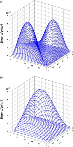
We consider (47) $u(x,y,t)=e^{-2{\pi }^{2}t}\sin [\pi (x+y-1)],S(x,y,t)=0,$(47) where $(x,y)\in [0,1{]}^2$ and we take $t_f=1$, and m = 1 in Equation (17(17) $g(x,y)=H(x,y)+\sum _{j=1}^m\sum _{k=1}^m{b}_{jk}\sin \frac{j\pi x}{a}\sin \frac{k\pi y}{b},$(17) ). As shown in Figure 1(a), the maximum error in the solution of $u(x,y,t_f)$ is $8.14\times {10}^{-10}$.

Figure 1. For (a) Example 1 and (b) Example 2 of the 2D FHCPs solved by the closed-form series solution, showing the absolute errors.

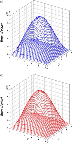
In order to test the stability of the analytic solution we add a large noise s = 0.5 in Equation (46(46) $\hat{f}(x_i,y_j)=f(x_i,y_j)+sR(i,j),$(46) ), and simultaneously we extend to a large domain with a = b = 10 and $t_f=10$. We take m = 1 in Equation (17(17) $g(x,y)=H(x,y)+\sum _{j=1}^m\sum _{k=1}^m{b}_{jk}\sin \frac{j\pi x}{a}\sin \frac{k\pi y}{b},$(17) ), and as shown in Figure 2(a), it is interesting that the maximum error in the solution of $u(x,y,t_f)$ is still small with $9.086\times {10}^{-5}$, even the absolute noise is large up to s = 0.5.

5.2. Example 2

We consider (48) $u(x,y,t)=e^{-t}(3x{y}^2-x^3),S(x,y,t)=e^{-t}(x^3-3x{y}^2),$(48) where $(x,y)\in [0,1{]}^2$ and we take $t_f=2$. As shown in Figure 1(b), the maximum error in the solution of $u(x,y,t_f)$ is $4.99\times {10}^{-9}$, where we only take m = 1 in Equation (17(17) $g(x,y)=H(x,y)+\sum _{j=1}^m\sum _{k=1}^m{b}_{jk}\sin \frac{j\pi x}{a}\sin \frac{k\pi y}{b},$(17) ).

We extend to a large domain with a = b = 10 and $t_f=10$. We take m = 1 in Equation (17(17) $g(x,y)=H(x,y)+\sum _{j=1}^m\sum _{k=1}^m{b}_{jk}\sin \frac{j\pi x}{a}\sin \frac{k\pi y}{b},$(17) ), and as shown in Figure 2(b), it is interesting that the maximum error in the solution of $u(x,y,t_f)$ is still small with $9.086\times {10}^{-5}$, even the absolute noise is large up to s = 0.5.

Figure 2. For (a) Example 1 and (b) Example 2 of the 2D FHCPs with large domain and large noise, showing the absolute errors.

The above two examples reveal that the present analytic series solution for the forward heat conduction problems is very accurate. Only a few terms in the series solution can lead to a high-order accurate solution.

6. Numerical tests of the 2D BHCP

For the BHCP, we assume that the given final temperature data are polluted by a random noise (49) $\hat{g}(x_i,y_j)=g(x_i,y_j)[1+sR(i,j)],$(49) where s is the intensity of relative noise and $R(i,j)\in [-1,1]$ are random numbers.

6.1. Example 3

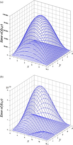
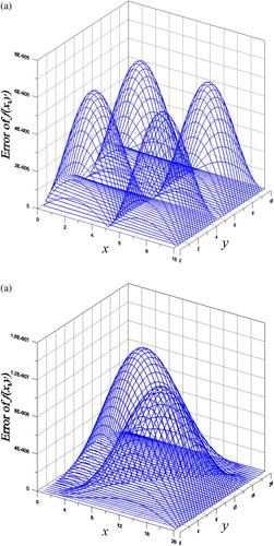
We first consider (50) $u(x,y,t)=e^{-t}(\cos x+\sin y),S(x,y,t)=0,$(50) in a large spatial temporal domain with a = b = 10 and $t_f=5$. As shown in Figure 3(a), the maximum error in the recovery of initial value is $2.36\times {10}^{-6}$, where we take m = 1, $n_0=2$ and $\alpha =0$. We increase the domain to a large one with a = b = 20 and $t_f=100$. As shown in Figure 3(b), the maximum error in the recovery of initial value is $3.846\times {10}^{-10}$, where we take m = 2, $n_0=2$ and $\alpha ={10}^{-5}$. It is amazing that high accuracy can be achieved although a relative random noise with a relative intensity s = 0.2 was added on the final time condition and a large time span is considered.

Figure 3. For Example 3 of a 2D BHCP solved by the closed-form series solution, showing the absolute errors for two cases.

In Table 1, we compare the maximum errors in the recovery of initial values with regularization and without considering regularization. It can be seen that m = 5 is not better than m = 2. Without considering regularization, the solution is unstable, which leads to an unreasonable error 2084530.28.

Table 1. For example 3 ($a=b=20,t_f=100,m=5$), the maximum errors in the recovery of initial values with regularization and without considering regularization.

$\alpha ={10}^{-5},n_0=2$	$\alpha ={10}^{-5},n_0=4$	Without regularization $\alpha =0$
$4.662\times {10}^{-1}$	$1.590\times {10}^{-1}$	2084530.28

6.2. Example 4

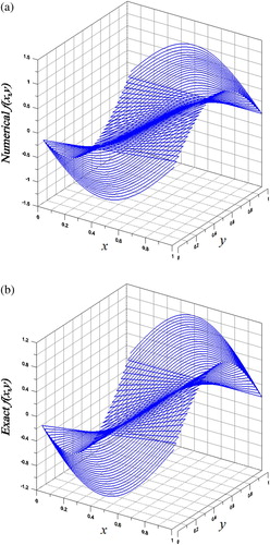
We consider (51) $u(x,y,t)=e^{-{\pi }^{2}t}\sin [\pi (x+y-5)],S(x,y,t)={\pi }^2{e}^{-{\pi }^{2}t}\sin [\pi (x+y-5)],$(51) in a spatial domain with a = b = 1 and $t_f=0.1$. We take m = 2, $n_0=2$, $\alpha ={10}^{-1}$ and s = 0.2. The maximum error as shown in Figure 4 is $3.35\times {10}^{-2}$, and in Figure 5, we compare the numerically recovered initial value with the exact one, which are close.

Figure 4. For Example 4 of a 2D BHCP solved by the closed-form series solution, showing the absolute errors.

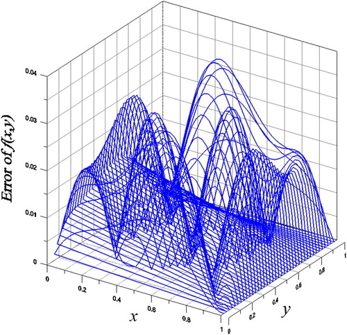
Figure 5. For Example 4 of a 2D BHCP solved by the new regularization technique, (a) numerical initial value, and (b) exact initial value.

In Table 2, we compare the maximum errors in the recovery of initial values with regularization and without considering regularization. It can be seen that m = 3 is not better than m = 2. Without considering regularization, the solution is unstable, which leads to an unreasonable error.

Table 2. For example 4 ($a=b=1,t_f=0.1,m=3$), the maximum errors in the recovery of initial values with regularization and without considering regularization.

$\alpha ={10}^{-1},n_0=1$	$\alpha ={10}^{-1},n_0=2$	Without regularization $\alpha =0$
1.197	1.845	1905.92

6.3. Example 5

Then we consider (52) $u(x,y,t)=e^{-t}(y^2-x^2),S(x,y,t)=e^{-t}(x^2-y^2),$(52) in a large spatial temporal domain with a = b = 10 and $t_f=20$. As shown in Figure 6(a), the maximum error in the recovery of initial value is $6.103\times {10}^{-5}$, where we take m = 2, $n_0=2$ and $\alpha ={10}^{-6}$. Upon noting that the maximum absolute value of the initial temperature to be recovered is 100, we can appreciate that very high accuracy can be achieved although a large relative intensity s = 0.2 of random noise was added on the final time condition and a large time span is considered.

Figure 6. For Example 5 of a 2D BHCP solved by the analytic series solution, showing the absolute errors for two cases.

In Table 3, we compare the maximum errors in the recovery of initial values with regularization and without considering regularization. It can be seen that m = 3 is not better than m = 2. Without considering regularization, the solution is unstable with an unreasonable error 18,465.935.

Table 3. For Example 5 ($a=b=10,t_f=20,m=3$), the maximum errors in the recovery of initial values with regularization and without considering regularization.

$\alpha ={10}^{-1},n_0=2$	$\alpha ={10}^{-1},n_0=3$	Without regularization $\alpha =0$
24.44	6.722	18465.935

Next we consider a more large domain of space-time with a = 20, b = 10 and $t_f=100$. As shown in Figure 6(b), the maximum error in the recovery of initial value is $1.23\times {10}^{-7}$, where we take m = 2, $n_0=2$ and $\alpha ={10}^{-6}$. Even a very large relative intensity s = 0.5 was added and a very large time span is considered, the analytic solution is very accurate, whose accuracy is never achieved by other methods.

The above examples reveal that the present analytic series solution with a simple regularization technique for the backward heat conduction problems is very accurate and robust against large noise. Only a few terms in the series solution can lead to a high-order accurate solution.

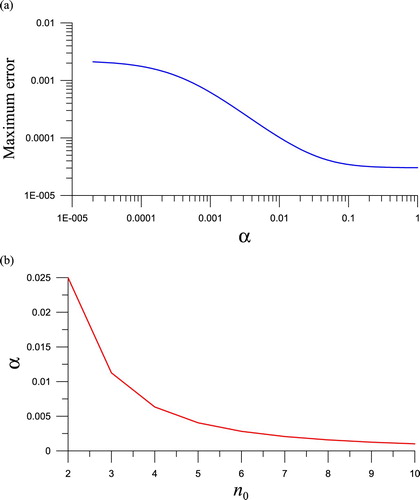
It is known that the selection of a suitable regularization parameter for the inverse problem is crucial [49], which may lead to a more accurate solution. A simple way to determine the regularization parameter can be achieved by plotting the curve of maximum error vs. regularization parameter. For Example 3 with a = 20, b = 10, $t_f=100$, s = 0.1 and m = 2, the curve is plotted in Figure 7(a), which tends to a stable maximum error when α approaches to one. In the recovery of initial value the first task is chosen a suitable value m, and then α and $n_0$. If $\alpha =0$ can generate good solution, we do not need to consider regularization. Otherwise, we need to consider α and $n_0$. Tables 1–3 reveal that the value $n_0$ is a crucial factor to influence the accuracy. If there exists no noise, basically the analytic solution approaches to the exact one as to be shown by the following Example 6. Under a noise s, we expect that the accuracy can be kept in the same order $A_{0}s$ where $A_0>0$. If a noise s is imposed on $g(x,y)$, by Equation (33(33) $\begin{array}{rl}{D}_{jk}:& ={\int }_0^b{\int }_0^{a}g(x,y)v^{jk}(x,y,t_f)\mathrm{d}x\mathrm{d}y-{\int }_0^{t_f}{\int }_0^b{\int }_0^a{v}^{jk}(x,y,t)S(x,y,t)\mathrm{d}x\mathrm{d}y\mathrm{d}t\\ & +{\int }_0^{t_f}{\int }_0^b{h}_2(y,t)v_x^{jk}(a,y,t)\mathrm{d}y\mathrm{d}t-{\int }_0^{t_f}{\int }_0^b{h}_1(y,t)v_x^{jk}(0,y,t)\mathrm{d}y\mathrm{d}t\\ & +{\int }_0^a{\int }_0^{t_f}{h}_4(x,t)v_y^{jk}(x,b,t)\mathrm{d}t\mathrm{d}x-{\int }_0^a{\int }_0^{t_f}{h}_3(x,t)v_y^{jk}(x,0,t)\mathrm{d}t\mathrm{d}x.\end{array}$(33) ), $D_{jk}$ will have an error due to s, when we suppose that other integration errors can be neglected. As shown in Equation (34(34) $a_{jk}^{\alpha }=\{\begin{array}{l}{\displaystyle {\displaystyle \frac{4}{ab}}[D_{jk}\exp ({\lambda }_{jk}{t}_f)-{\int }_0^b{\int }_0^a\sin {\displaystyle \frac{j\pi x}{a}}\sin \frac{k\pi y}{b}F(x,y)\mathrm{d}x\mathrm{d}y],\text{if}j\text{or}k<n_0,}\\ {\displaystyle \frac{4}{ab}[\frac{D_{jk}}{\exp (-{\lambda }_{jk}{t}_f)+\alpha }-{\int }_0^b{\int }_0^a\sin \frac{j\pi x}{a}\sin \frac{k\pi y}{b}F(x,y)\mathrm{d}x\mathrm{d}y],\text{if}j\text{and}k\ge n_0.}\end{array}$(34) ), the major contribution to enlarge the error in $D_{jk}$ is the term with $j=k=n_0$. Then, when we use the above principle and integrate the first term in Equation (33(33) $\begin{array}{rl}{D}_{jk}:& ={\int }_0^b{\int }_0^{a}g(x,y)v^{jk}(x,y,t_f)\mathrm{d}x\mathrm{d}y-{\int }_0^{t_f}{\int }_0^b{\int }_0^a{v}^{jk}(x,y,t)S(x,y,t)\mathrm{d}x\mathrm{d}y\mathrm{d}t\\ & +{\int }_0^{t_f}{\int }_0^b{h}_2(y,t)v_x^{jk}(a,y,t)\mathrm{d}y\mathrm{d}t-{\int }_0^{t_f}{\int }_0^b{h}_1(y,t)v_x^{jk}(0,y,t)\mathrm{d}y\mathrm{d}t\\ & +{\int }_0^a{\int }_0^{t_f}{h}_4(x,t)v_y^{jk}(x,b,t)\mathrm{d}t\mathrm{d}x-{\int }_0^a{\int }_0^{t_f}{h}_3(x,t)v_y^{jk}(x,0,t)\mathrm{d}t\mathrm{d}x.\end{array}$(33) ), we can derive (53) $\frac{s}{(e^{-2n_0^2{t}_f}+\alpha )n_0^2{\pi }^2}=A_{0}s,$(53) where the geometric sizes are supposed to be $a=b=\pi$. Accordingly, we can derive the following formula to determine the regularization parameter: (54) $\alpha =\frac{1}{n_0^2{\pi }^2{A}_0}-e^{-2n_0^2{t}_f}.$(54) With the parameters $t_f=1$ and $A_0=1$, we plot the curve of α vs. $n_0$ in Figure 7(b). When $n_0$ increases, α tends to a stable value.

Figure 7. (a) For Example 5 showing the maximum error vs. regularization parameter, and (b) in general, the regularization parameter vs. $n_0$.

We employ the above rule with $A_0=0.5$ to solve Example 3 again, where we take a = b = 20, $t_f=100$, s = 0.1 and m = 4. In Table 4, we compare the maximum errors in the recovery of initial values with regularization parameter determined by Equation (54(54) $\alpha =\frac{1}{n_0^2{\pi }^2{A}_0}-e^{-2n_0^2{t}_f}.$(54) ), where we take $A_0=0.5$. The solution is convergent fast with the maximum error being $4.550\times {10}^{-10}$ when $n_0=4$.

Table 4. For Example 3 ($a=b=20,t_f=100,s=0.1,m=4$), the maximum errors in the recovery of initial values with regularization are convergent.

$n_0$	1	2	3	4
α	$2.026\times {10}^{-1}$	$5.066\times {10}^{-2}$	$2.252\times {10}^{-2}$	$1.267\times {10}^{-2}$
Maximum error	$3.604\times {10}^{-1}$	$1.364\times {10}^{-1}$	$1.182\times {10}^{-1}$	$4.550\times {10}^{-10}$

As shown by Equation (12(12) ${\lambda }_{jk}=\frac{j^2{\pi }^2}{a^2}+\frac{k^2{\pi }^2}{b^2}$(12) ), when the domain is increased with large a and b, the eigenvalue is decreased. Therefore, we can take more eigenfunctions in the series solution (24(24) $f(x,y)=F(x,y)+\sum _{j=1}^m\sum _{k=1}^m{a}_{jk}\sin \frac{j\pi x}{a}\sin \frac{k\pi y}{b},$(24) ) to increase the accuracy and also can avoid the instability happening too earlier, due to $\exp ({\lambda }_{jk}{t}_f)$ in Equation (32(32) $a_{jk}=\frac{4}{ab}[\exp ({\lambda }_{jk}{t}_f)D_{jk}-{\int }_0^b{\int }_0^a\sin \frac{j\pi x}{a}\sin \frac{k\pi y}{b}F(x,y)\mathrm{d}x\mathrm{d}y],j,k=1,\dots ,m,$(32) ).

6.4. Example 6

Finally, we use the following example to demonstrate that the new analytic solution is just the exact solution if noise is not considered (55) $u(x,y,t)=\exp [-{\pi }^{2}t(\frac{1}{a^2}+\frac{1}{b^2})]\sin \frac{\pi x}{a}\sin \frac{\pi y}{b}.$(55) From Equation (55(55) $u(x,y,t)=\exp [-{\pi }^{2}t(\frac{1}{a^2}+\frac{1}{b^2})]\sin \frac{\pi x}{a}\sin \frac{\pi y}{b}.$(55) ), it follows that $h_1=0,h_2=0,h_3=0,h_4=0,S=0.$ Inserting them into Equation (21(21) $\begin{array}{rl}F(x,y)& =(1-\frac{x}{a})[h_1(y,0)-(1-\frac{y}{b})h_3(0,0)-\frac{y}{b}{h}_4(0,0)]\\ & +\frac{x}{a}[h_2(y,0)-(1-\frac{y}{b})h_3(a,0)-\frac{y}{b}{h}_4(a,0)]\\ & +(1-\frac{y}{b})h_3(x,0)+\frac{y}{b}{h}_4(x,0),\end{array}$(21) ), we have F = 0, which together with S = 0 being inserted into Equations (32(32) $a_{jk}=\frac{4}{ab}[\exp ({\lambda }_{jk}{t}_f)D_{jk}-{\int }_0^b{\int }_0^a\sin \frac{j\pi x}{a}\sin \frac{k\pi y}{b}F(x,y)\mathrm{d}x\mathrm{d}y],j,k=1,\dots ,m,$(32) ) and (33(33) $\begin{array}{rl}{D}_{jk}:& ={\int }_0^b{\int }_0^{a}g(x,y)v^{jk}(x,y,t_f)\mathrm{d}x\mathrm{d}y-{\int }_0^{t_f}{\int }_0^b{\int }_0^a{v}^{jk}(x,y,t)S(x,y,t)\mathrm{d}x\mathrm{d}y\mathrm{d}t\\ & +{\int }_0^{t_f}{\int }_0^b{h}_2(y,t)v_x^{jk}(a,y,t)\mathrm{d}y\mathrm{d}t-{\int }_0^{t_f}{\int }_0^b{h}_1(y,t)v_x^{jk}(0,y,t)\mathrm{d}y\mathrm{d}t\\ & +{\int }_0^a{\int }_0^{t_f}{h}_4(x,t)v_y^{jk}(x,b,t)\mathrm{d}t\mathrm{d}x-{\int }_0^a{\int }_0^{t_f}{h}_3(x,t)v_y^{jk}(x,0,t)\mathrm{d}t\mathrm{d}x.\end{array}$(33) ), generates (56) $\begin{array}{rl}{a}_{jk}& =\frac{4}{ab}\exp ({\lambda }_{jk}{t}_f)D_{jk},\end{array}$(56) (57) $\begin{array}{rl}{D}_{jk}:& ={\int }_0^b{\int }_0^{a}g(x,y)v^{jk}(x,y,t_f)\mathrm{d}x\mathrm{d}y.\end{array}$(57) By using the final time function obtained from Equation (55(55) $u(x,y,t)=\exp [-{\pi }^{2}t(\frac{1}{a^2}+\frac{1}{b^2})]\sin \frac{\pi x}{a}\sin \frac{\pi y}{b}.$(55) ) (58) $g(x,y)=u(x,y,t_f)=\exp [-{\pi }^2{t}_f(\frac{1}{a^2}+\frac{1}{b^2})]\sin \frac{\pi x}{a}\sin \frac{\pi y}{b},$(58) and inserting Equations (11(11) $v^{jk}(x,y,t)=\exp [{\lambda }_{jk}(t-t_f)]\sin \frac{j\pi x}{a}\sin \frac{k\pi y}{b},$(11) ) and (12(12) ${\lambda }_{jk}=\frac{j^2{\pi }^2}{a^2}+\frac{k^2{\pi }^2}{b^2}$(12) ) into Equations (56(56) $\begin{array}{rl}{a}_{jk}& =\frac{4}{ab}\exp ({\lambda }_{jk}{t}_f)D_{jk},\end{array}$(56) ) and (57(57) $\begin{array}{rl}{D}_{jk}:& ={\int }_0^b{\int }_0^{a}g(x,y)v^{jk}(x,y,t_f)\mathrm{d}x\mathrm{d}y.\end{array}$(57) ), it leads to (59) $\begin{array}{rl}{D}_{11}:& =\frac{ab}{4}\exp [-{\pi }^2{t}_f(\frac{1}{a^2}+\frac{1}{b^2})],D_{jk}=0,\text{if}j\ne 1,k\ne 1,\end{array}$(59) (60) $\begin{array}{rl}{a}_{11}& =\frac{4}{ab}\exp ({\lambda }_{11}{t}_f)\frac{ab}{4}\exp [-{\pi }^2{t}_f(\frac{1}{a^2}+\frac{1}{b^2})]=1,a_{jk}=0,\text{if}j\ne 1,k\ne 1,\end{array}$(60) where the orthogonality of sinusoidal functions was employed in the derivation.

By Equations (24(24) $f(x,y)=F(x,y)+\sum _{j=1}^m\sum _{k=1}^m{a}_{jk}\sin \frac{j\pi x}{a}\sin \frac{k\pi y}{b},$(24) ) and (60(60) $\begin{array}{rl}{a}_{11}& =\frac{4}{ab}\exp ({\lambda }_{11}{t}_f)\frac{ab}{4}\exp [-{\pi }^2{t}_f(\frac{1}{a^2}+\frac{1}{b^2})]=1,a_{jk}=0,\text{if}j\ne 1,k\ne 1,\end{array}$(60) ), we can recover the initial function to be (61) $f(x,y)=\sin \frac{\pi x}{a}\sin \frac{\pi y}{b},$(61) which is the exact one after inserting t = 0 into Equation (55(55) $u(x,y,t)=\exp [-{\pi }^{2}t(\frac{1}{a^2}+\frac{1}{b^2})]\sin \frac{\pi x}{a}\sin \frac{\pi y}{b}.$(55) ).

7. Conclusions

In this paper, we have derived a domain/boundary integral equation method to solve the two-dimensional heat conduction problems with source terms and under the non-homogeneous boundary conditions. The stable adjoint Trefftz test functions were derived, such that the analytic solutions in terms of homogenization functions and closed-form series are available for both the forward heat conduction problem (FHCP) and the backward heat conduction problem (BHCP). These solutions were obtained for the first time in the literature. For the 2D FHCP, the numerical examples revealed that the new method is very accurate, without suffering from the time integration error and the propagation of error. In order to stably solve the 2D BHCP in a large space-time domain we have introduced a simple spring-damping regularization technique in the analytic series solution. Numerical tests were given, which confirmed that the new method was applicable to the 2D BHCPs with large time-span. Although the input measured final time data were polluted by a large noise up to the level $20\mathrm{\%}$, and $t_f$ is large up to 100, the presented analytic series solution is very accurate to recover the initial temperature with an error in the order from ${10}^{-2}$ to ${10}^{-10}$.

Acknowledgments

C.-S. Liu is grateful to the twelfth Guanghua Engineering Science and Technology Prize.

Disclosure statement

No potential conflict of interest was reported by the author(s).

Additional information

Funding

The Fundamental Research Funds for the Central Universities [grant number 2017B05714] for the financial support to the first author are highly appreciated.

References

- Wilson EL, Nickell RE. Application of the finite element method to heat conduction analysis. Nucl Eng Des. 1966;4(3):276–286.
- Zienkiewicz OC, Taylor RL, Zhu JZ. The finite element method: its basis and fundamentals. Amsterdam (Netherlands): Butterworth-Heinemann; 2005.
- Li W, Yu B, Wang XR, et al. A finite volume method for cylindrical heat conduction problems based on local analytical solution. Int J Heat Mass Transfer. 2012;55:5570–5582.
- Wrobel LC, Brebbia CA. The dual reciprocity boundary element formulation for nonlinear diffusion problems. Comput Meth Appl Mech Eng. 1987;65:147–164.
- Atalay MA, Aydin ED, Aydin M. Multi-region heat conduction problems by boundary element method. Int J Heat Mass Transfer. 2004;47:1549–1553.
- Chen CS, Golberg MA, Hon YC. The method of fundamental solutions and quasi-Monte-Carlo method for diffusion equations. Int J Numer Meth Eng. 1998;43:1421–1435.
- Chantasiriwan S. Methods of fundamental solutions for time-dependent heat conduction problems. Int J Numer Meth Eng. 2006;66:147–165.
- Johansson BT, Lesnic D. A method of fundamental solutions for transient heat conduction. Eng Anal Bound Elem. 2008;32:697–703.
- Johansson BT, Lesnic D, Reeve T. A method of fundamental solutions for two dimensional heat conduction. Int J Comput Math. 2011;88:1697–1713.
- Cannon JR. The backward continuation in time by numerical means of the solution of the heat equation in a rectangle [MA Thesis]. Houston (TX): Rice University; 1960.
- Cannon JR. Numerical continuation backwards in time for solutions of the heat equation and numerical continuation of solutions of Laplace's equation in a half space. Brookhaven National Laboratory, New York; 1964. (Report number 8185).
- Cannon JR. Some numerical results for the solution of the heat equation backwards in time. In: Greenspan D, editor. Numerical solutions of nonlinear differential equations. New York (NY): John Wiley; 1966. p. 21–54.
- Han H, Ingham DB, Yuan Y. The boundary element method for the solution of the backward heat conduction equation. J Comput Phys. 1995;116:292–299.
- Mera NS, Elliott L, Ingham DB, et al. An iterative boundary element method for solving the one-dimensional backward heat conduction problem. Int J Heat Mass Transfer. 2001;44:1937–1946.
- Mera NS, Elliott L, Ingham DB. An inversion method with decreasing regularization for the backward heat conduction problem. Numer Heat Transfer B. 2002;42:215–230.
- Muniz WB, de Campos Velho HF, Ramos FM. A comparison of some inverse methods for estimating the initial condition of the heat equation. J Comput Appl Math. 1999;103:145–163.
- Muniz WB, Ramos FM, de Campos Velho HF. Entropy- and Tikhonov-based regularization techniques applied to the backward heat equation. Int J Comput Math. 2000;40:1071–1084.
- Kirkup SM, Wadsworth M. Solution of inverse diffusion problems by operator-splitting methods. Appl Math Model. 2002;26:1003–1018.
- Iijima K. Numerical solution of backward heat conduction problems by a high order lattice-free finite difference method. J Chinese Inst Eng. 2004;27:611–620.
- Hon YC, Li M. A discrepancy principle for the source points location in using the MFS for solving the BHCP. Int J Comput Meth. 2009;6:181–197.
- Tsai CH, Young DL, Kolibal J. An analysis of backward heat conduction problems using the time evolution method of fundamental solutions. Comput Model Eng Sci. 2010;66:53–71.
- Qian Z, Fu CL, Shi R. A modified method for a backward heat conduction problem. Appl Math Comput. 2007;185:564–573.
- Fu CL, Xiong XT, Qian Z. Fourier regularization for a backward heat equation. J Math Anal Appl. 2007;331:472–480.
- Xiong XT, Fu CL, Qian Z. On three spectral regularization methods for a backward heat conduction problem. J Korean Math Soc. 2007;44:1281–1290.
- Li M, Jiang T, Hon YC. A meshless method based on RBFs method for nonhomogeneous backward heat conduction problem. Eng Anal Bound Elem. 2010;34:785–792.
- Clark GW, Oppenheimer SF. Quasireversibility methods for non-well-posed problems. Electron J Differ Eqs. 1994;1994:1–9.
- Ames KA, Clark GW, Epperson JF, et al. A comparison of regularizations for an ill-posed problem. Math Comput. 1998;67:1451–1471.
- Chang JR, Liu C-S, Chang CW. A new shooting method for quasi-boundary regularization of backward heat conduction problems. Int J Heat Mass Transfer. 2007;50:2325–2332.
- Chen YW. A highly accurate backward-forward algorithm for multi-dimensional backward heat conduction problems in fictitious time domains. Int J Heat Mass Transfer. 2018;120:499–514.
- Liu C-S. Group preserving scheme for backward heat conduction problems. Int J Heat Mass Transfer. 2004;47:2567–2576.
- Liu C-S, Chang CW, Chang JR. Past cone dynamics and backward group preserving schemes for backward heat conduction problems. Comput Model Eng Sci. 2006;12:67–81.
- Chang CW, Liu C-S, Chang JR. A quasi-boundary semi-analytical method for backward heat conduction problems. J Chinese Inst Eng. 2010;33:163–175.
- Liu C-S. A new method for Fredholm integral equations of 1D backward heat conduction problems. Comput Model Eng Sci. 2009;47:1–21.
- Chang CW, Liu C-S, Chang JR. A new shooting method for quasi-boundary regularization of multi-dimensional backward heat conduction problems. J Chinese Inst Eng. 2009;32:307–318.
- Liu C-S. A highly accurate LGSM for severely ill-posed BHCP under a large noise on the final time data. Int J Heat Mass Transfer. 2010;53:4132–4140.
- Chang CW, Liu C-S. A new algorithm for direct and backward problems of heat conduction equation. Int J Heat Mass Transfer. 2010;52:5552–5569.
- Liu C-S. A self-adaptive LGSM to recover initial condition or heat source of one-dimensional heat conduction by using only minimal boundary data. Int J Heat Mass Transfer. 2011;54:1305–1312.
- Liu C-S. The method of fundamental solutions for solving the backward heat conduction problem with conditioning by a new post-conditioner. Numer Heat Transfer B. 2011;60:57–72.
- Liu C-S, Chang CW. A simple algorithm for solving Cauchy problem of nonlinear heat equation without initial value. Int J Heat Mass Transfer. 2015;80:562–569.
- Liu C-S, Chang CW. Nonlinear problems with unknown initial temperature and without final temperature, solved by the GL(N,R) shooting method. Int J Heat Mass Transfer. 2015;83:655–678.
- Liu C-S, Kuo CL, Chang JR. Recovering a heat source and initial value by a Lie-group differential algebraic equations method. Numer Heat Transfer B. 2015;67:231–254.
- Liu C-S. Lie-group differential algebraic equations method to recover heat source in a Cauchy problem with analytic continuation data. Int J Heat Mass Transfer. 2014;78:538–547.
- Liu C-S. A multiple/scale/direction polynomial Trefftz method for solving the BHCP in high-dimensional arbitrary simply-connected domains. Int J Heat Mass Transfer. 2016;92:970–978.
- Jarny Y, Ozisik MN, Bardon JP. A general optimization method using adjoint equation for solving multidimensional inverse heat conduction. Int J Heat Mass Transfer. 1991;34:2911–2919.
- Mera NS. The method of fundamental solutions for the backward heat conduction problem. Inverse Probl Sci Eng. 2005;13:65–78.
- Liu C-S, Wang P. An analytic adjoint Trefftz method for solving the singular parabolic convection-diffusion equation and initial pollution profile problem. Int J Heat Mass Transfer. 2016;101:1177–1184.
- Liu C-S, Kuo CL. A spring-damping regularization and a novel Lie-group integration method for nonlinear inverse Cauchy problems. Comput Model Eng Sci. 2011;77:57–80.
- Liu C-S, Kuo CL, Liu D. The spring-damping regularization method and the Lie-group shooting method for inverse Cauchy problems. Comput Mater Contin. 2011;24:105–123.
- Kirsch A. An introduction to the mathematical theory of inverse problems. New York (NY): Springer; 2011.