Formulation of equation error estimator using measured displacement de-noised by temporal–spatial filter for system identification of elastic solids

ABSTRACT

This paper presents a new class of the equation error estimator using de-noised displacement by the temporal–spatial filter for the system identification in an elastic solid. The finite element method is employed to discretize the equation of motion for an elastic solid, and the Young’s modulus of each finite element is estimated by the proposed approach. The temporal–spatial filter is applied to de-noise measured nodal displacements and to reconstruct nodal accelerations. The equation of motion modified for the de-noised dynamic responses is derived, and the equation error estimator (EEE) for the system identification is defined with the modified equation of motion. The proposed EEE represents the residual error of the modified equation of motion over a measurement interval, and results in a nonlinear equation, which is solved by the successive substitution method. The sensitivity of the temporal–spatial filter required to solve the nonlinear equation is derived by the direction differentiation of the analytical expressions of the filter. The validity and accuracy of the proposed approach are tested through numerical simulation studies. It is shown that the proposed method yields accurate and stable solutions without regularization for all cases tested in this study.

KEYWORDS:

• T-S filter
• regularization
• de-noising
• system identification
• equation of motion
• measured displacement
• sensitivity
• equation error estimator
• residual error

SUBJECT CLASSIFICATION CODE:

• 74B05

1. Introduction

Over the last couple of decades, a great deal of effort has been made to develop stable system identification (SI) schemes in various fields such as medical imaging [1,2] and damage detection of structures [3–12]. Traditionally, the output error estimator (OEE), which is the least-square errors between measured and calculated responses, is widely adopted in SI schemes because of the sparseness of measured data [7–12]. The OEE usually results in a nonlinear optimization problem, which requires iteration solution schemes. Meanwhile, SI problems are also described with the equation error estimator (EEE), which is the least-square residual error of a discretized governing equation [1–6]. The EEE has an advantage over the OEE because the EEE yields a quadratic problem if the governing equation is linear. However, system responses at all degrees of freedom of the discretized governing equation should be fully measured to adopt the EEE, which limits its applicability. Taking advantage of recent advances in measurement technologies, the EEE has been frequently employed in various SI problems, especially for problems defined in relatively small domains. The medical imaging and damage detection within a small domain may be typical application fields of the EEE [1,2].

Since SI problems are ill-posed regardless of the type of the error estimator, a stabilization scheme should be employed to obtain physically meaningful and numerically stable solutions [13,14]. The regularization scheme, which imposes the solution space of a SI problem on an error estimator, is the most popular approach adopted to alleviate the ill-posedness of SI problems [5,6,8–12]. Although the regularization scheme has been successfully applied in various engineering fields, the regularization scheme has two major drawbacks in real applications. One is the ambiguity in selecting an optimal regularization factor [5,6,8–12], and the other is the loss of information in measured data, which may cause smeared solutions. Moreover, it is rather difficult to define the regularity condition as a single regularization function for problems defined in the temporal and spatial domain.

The inherent instabilities of SI problems are triggered by noise components in measured data, which are not in the admissible solution space of a given system. Recognizing this fact, the de-noising approach may also be utilized as an alternative to the regularization scheme. In this method, noise in the measured data is filtered out using properly defined digital filters, and then the SI problem is solved using the de-noised data. Since the EEE is based on the equation of motion with the inertia and strain term, noise should be suppressed in the temporal as well as spatial domain. Park et al. [1,2] adopted a similar approach to identify inclusions in human tissues. They applied a de-noising filter imposing the continuity and incompressibility of displacement in the spatial domain with three regularization factors to measured displacements, but consider neither temporal de-nosing nor the change in the equation of motion caused by the filter. No explicit algorithm to determine the three regularization factors is presented in the study.

This paper formulates a new class of the EEE, which is referred to as the T-S EEE herein after, using the measured displacement and reconstructed acceleration de-noised by the temporal–spatial (T-S) filter proposed by Park and Lee [15]. The new concept adopted in this study is the use of de-noised measurement by the T-S filter in place of a regularization scheme to obtain physically meaningful and numerically stable solutions of system identification. The T-S EEE is free from the two drawbacks of the regularization scheme. The target frequency for the T-S filter, which plays the same role as the regularization factor in the regularization scheme, is clearly defined. As the stabilization effect is provided by the T-S filter rather than a regularization function added to the EEE, no further stabilization scheme is required, and the original characteristics of the EEE are retained during system identification. Therefore, physically meaningful information in measurement as well as the original characteristics of a given system can be utilized in system identification as much as possible.

The equation of motion of an elastic solid is discretized by the finite element method. The Young’s modulus of each finite element is identified by the minimization of the EEE based on the equation of motion modified for filtered dynamic responses. The proposed EEE is defined as the time integration of the 2-norm of the residual error of the modified equation of motion over a measurement interval. Dissimilar to the conventional EEE, the minimization of the proposed EEE becomes a nonlinear optimization problem because the T-S filter itself is a function of the Young’s modulus of each finite element. A successive substitution method is employed to solve the nonlinear problem, and the sensitivity of the T-S filter required in the solution scheme is calculated by the direct differentiation of its analytical expression.

A series of numerical simulation studies on the identification of inclusions in a finite elastic solid is performed to demonstrate the validity and accuracy of the proposed approach. A soft and hard inclusion, which have lower and higher Young’s modulus than that of a matrix material, respectively, are considered. The proposed EEE is tested for both free- and forced-vibration conditions. The soft inclusion is identifiable by the conventional EEE as well as the proposed approach, while the conventional EEE does not yield accurate solutions for the hard inclusion. On the other hand, the proposed approach estimates the location, size and Young’s modulus of the hard inclusion. Detailed discussions on the stabilization effect provided by the regularization scheme and proposed approach are presented. The general applicability of the proposed EEE is confirmed by the identification of various types of hard inclusions.

2. Inverse problem with equation error estimator

2.1. Problem definition

The equation of motion, boundary and initial conditions of an elastic solid shown in Figure 1 are defined as follows: $C_{ijkl}\frac{{\mathrm{\partial }}^2{u}_k}{\mathrm{\partial }{x}_j\mathrm{\partial }{x}_l}-\rho \frac{{\mathrm{\partial }}^2{u}_i}{\mathrm{\partial }{t}^2}=0\text{ in }V$ $u_i={\overline{u}}_i\text{ on }{S}_u\text{ and }{T}_i={\overline{T}}_i\text{ on }{S}_T$ (1) $u_i(\mathbf{\text{x}})=u_i^0(\mathbf{\text{x}})\text{ and }\frac{\mathrm{\partial }{u}_i}{\mathrm{\partial }t}=v_i^0(\mathbf{\text{x}})\text{ at }t=0\text{ for }\mathrm{\forall }\mathbf{\text{x}}\in V$(1) where V, $u_i$, $C_{ijkl}$, ρ and x are the domain, displacement, elasticity tensor, mass density and position vector, respectively. The displacement and traction prescribed on S_u and S_T are denoted as ${\overline{u}}_i$ and ${\overline{T}}_i$, respectively, while the initial conditions for displacement and velocity are given by the corresponding variables with superscript 0. Damping is not considered in the SI. The discretized equation of motion is written in a usual matrix form by applying a standard finite element (FE) procedure [16]. (2) $\mathbf{\text{MA}}(t)+\mathbf{\text{KU}}(t)=\mathbf{\text{P}}$(2) where M, K and P are the mass, stiffness matrix and equivalent nodal force vector, while A(t) and U(t) are the nodal acceleration and displacement vector of the FE model at time t, respectively.

Figure 1. An elastic solid with an inclusion and its finite element model.

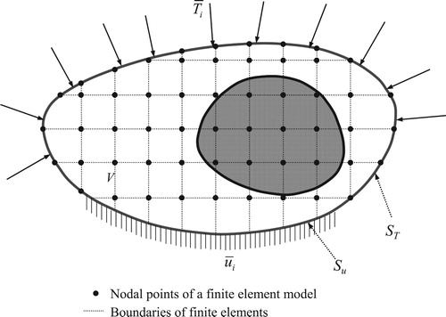
Suppose that the body contains an inclusion with an unknown, time-invariant Young’s modulus as shown in Figure 1, and that all components of displacement and acceleration at each nodal point of the FE model are completely measured. The residual error of Equation (2) at time t is written as a function of the unknown Young’s moduli of finite elements. (3) $\begin{array}{rl}\mathbf{\text{R}}(\mathbf{\text{E}},t)& =\mathbf{\text{M}}\overline{\mathbf{\text{A}}}(t)+\sum _e{E}^e{\mathbf{\text{k}}}_1^e{\overline{\mathbf{\text{U}}}}^e(t)-\mathbf{\text{P}}\\ & =\mathbf{\text{M}}\overline{\mathbf{\text{A}}}(t)+{\overline{\mathbf{\text{K}}}}_1\mathbf{\text{E}}-\mathbf{\text{P}}\end{array}$(3) Here, $E^e$, ${\mathbf{\text{k}}}_1^e$ and ${\overline{\mathbf{\text{U}}}}^e$ are the Young’s modulus, stiffness matrix corresponding to the unit Young’s modulus and measured displacements at the nodes of element e, respectively, while E is the vector containing the unknown Young’s moduli of all elements in the FE model. The assembly operator for Young’s modulus vector is denoted as $\sum _e$in Equation (3). The unknown Young’s modulus of each element is estimated by minimizing the EEE defined as the time integration of the 2-norm of the residual error in Equation (3) over a measurement interval. (4) $\underset{\mathbf{\text{E}}}{\text{Min }\mathrm{\Pi }}=\frac{1}{2}{\int }_{t_i}^{t_f}||\mathbf{\text{M}}\overline{\mathbf{\text{A}}}(t)+{\overline{\mathbf{\text{K}}}}_1\mathbf{\text{E}}-\mathbf{\text{P}}|{|}_2^{2}dt$(4) where t_i and t_f represent the initial and final time of the measurement interval, respectively. If noise is not included in measured data and discretization error is negligible, Equation (4) yields the exact solution of the Young’s modulus vector.

Two difficulties are expected in adopting the EEE in Equation (4) for the SI. That is, some kinds of noise are always presented in measurement, and both displacement and acceleration cannot be measured simultaneously at a same spatial point. Therefore, when the nodal displacement is measured, the nodal acceleration should be estimated by a numerical differentiation scheme, which severely amplifies the noise in the measured displacement in the temporal domain [17]. In addition, the strain components, which are the spatial derivatives of displacement, in the stiffness matrix are also polluted by amplified noise in the spatial domain. Therefore, a stabilization scheme should be employed to solve SI problems defined by the EEE as those by the OEE.

Regularization schemes are successfully employed in various types of SI problems to suppress the effect of noise on the solution [5,6,8–12]. In the regularization scheme, a regularization function is added to an error estimator as a penalty function to define the solution space of an SI problem. Meanwhile, the instability of an SI problem can be effectively eliminated by de-nosing measured displacement with a proper filter in the temporal and spatial domain because the instability of an SI problem is basically caused by noise in the measurement. A robust de-noising filter, which is referred to as the T-S filter, has been recently proposed [15], and this study adopts the T-S filter to de-noise measured displacement.

2.2. Temporal–spatial filter

The explicit expressions of the T-S filter are required for the formulation of the EEE proposed in this study, and thus the filter is introduced briefly in this section. Details of the forthcoming derivation have been presented in the work by Park and Lee [15]. The temporal filter is defined by the following minimization problem in a moving time window: (5) $\underset{{\tilde{U}}_j}{min}{\mathrm{\Pi }}_t=\frac{1}{2}{\int }_{t_1}^{t_2}{({\tilde{U}}_j-{\overline{U}}_j)}^{2}dt+\frac{{\lambda }_t\mathrm{\Delta }{t}^4}{2}{\int }_{t_1}^{t_2}{\left(\frac{d^2{\tilde{U}}_j}{d{t}^2}\right)}^{2}dt\text{ for}j=1,\cdots ,ndof$(5) where ${\tilde{U}}_j$, ${\overline{U}}_j$, ${\lambda }_t$, $\mathrm{\Delta }t$, ndof, $t{}_1$ and $t{}_2$ are the temporally de-noised, measured displacement of the j-th observation point, temporal regularization factor, sampling interval, number of degrees of freedom, the starting and ending time of the time window, respectively. The temporal filter is derived by taking variation of Equation (5) and discretizing the time window using an FE model, in which each sampling interval serves as a finite element for a time window. The Hermitian and linear shape functions are adopted to interpolate the de-noised and measured displacement, respectively. The de-noised displacement in the temporal domain is obtained by solving the discretized temporal filter. (6) ${\widetilde{\mathbf{\text{U}}}}_j=({\mathbf{\text{M}}}_t+{\lambda }_t{\mathbf{\text{K}}}_t{)}^{-1}{\mathbf{\text{Q}}}_t{\overline{\mathbf{\text{U}}}}_j=\mathbf{\text{G}}{\overline{\mathbf{\text{U}}}}_j$(6) where ${\widetilde{\mathbf{\text{U}}}}_j$ and ${\overline{\mathbf{\text{U}}}}_j$ are the vectors of the temporally de-noised and measured displacements at all sampling times in a time window for the j-th observation point, respectively, while G represents the temporal filter matrix. The explicit expressions of the matrixes in Equation (6) are given in reference [15] in terms of the shape functions utilized to discretize Equation (5). The velocity field is obtained simultaneously with the de-noised displacement in the temporal filter because the nodal velocity is embedded as an unknown in Equation (6). The regularization factor of the temporal filter is defined as: (7) ${\lambda }_t=\frac{1}{{(2\pi \mathrm{\Delta }t{f}_T^{})}^4}\frac{1-{\alpha }_t}{{\alpha }_t}$(7) where α_t denotes the target accuracy of the temporal filter while f_T is the target frequency which is the highest meaningful frequency in the measured displacement.

Since the temporal filter uses the moving time-window technique proposed by Lee et al. [18], the de-noised displacement and reconstructed velocity at the centre of each time window are selected as those of the time window. Thus, only two rows of G corresponding to the centre node of a time window in Equation (6) are used to form the temporal filter. (8) $\begin{array}{r}{\tilde{U}}_j(t)=\sum _{p=-k_w}^{k_w}{G}_{2k_w+1,p+k_w+1}{\overline{U}}_j(t+p\mathrm{\Delta }t)\mathrm{and}{\tilde{V}}_j(t)=\sum _{p=-k_w}^{k_w}{G}_{2k_w+2,p+k_w+1}{\overline{U}}_j(t+p\mathrm{\Delta }t)\end{array}$(8) where $G_{j,k}$ and 2k_w denote the general entry of G and the total number of sampling intervals in a time window, respectively, while ${\tilde{V}}_j$ is the reconstructed velocity. Notice that the coefficients of the temporal filter in Equation (8) are constant for all time windows if a fixed time window size and sampling interval are employed in the filter. The reconstructed acceleration of the j-th observation point, ${\tilde{A}}_j$, is calculated by the central difference of the reconstructed velocity. (9) $\begin{array}{rl}{\tilde{A}}_j(t)& \approx \frac{{\tilde{V}}_j(t+\mathrm{\Delta }t)-{\tilde{V}}_j(t-\mathrm{\Delta }t)}{2\mathrm{\Delta }t}\\ & =\frac{1}{2\mathrm{\Delta }t}\sum _{p=-k_w}^{k_w}{G}_{2k_w+2,p+k_w+1}({\overline{U}}_j(t+(p+1)\mathrm{\Delta }t)-{\overline{U}}_j(t+(p-1)\mathrm{\Delta }t))\end{array}$(9) Since the coefficients of the temporal filter in Equation (8) for displacement are symmetry with respect to p, the transfer function for the filtered displacement, $H_t^u$ is written as follows: (10) $H_t^u=\sum _{p=-k_w}^{k_w}{G}_{2k_w+1,p+k_w+1}\text{cos(}\mathrm{\Delta }tp\omega )$(10)

The spatial filter is formed by the following minimization problem using the temporally de-noised displacement in Equation (8). (11) $\underset{{\hat{u}}_i}{min}\mathrm{\Pi }=\frac{1}{2}\frac{\rho }{\mathrm{\Delta }{t}^2}{\int }_V^{}({\hat{u}}_j-{\tilde{u}}_j)({\hat{u}}_j-{\tilde{u}}_j)dV+\frac{1}{2}{\lambda }_s{\int }_V^{}\frac{d{\hat{u}}_j}{d{x}_k}{C}_{jkmn}\frac{d{\hat{u}}_m}{d{x}_n}dV\text{for all}t$(11) where ${\lambda }_s$ is the spatial regularization factor, while ${\hat{u}}_j$ and ${\tilde{u}}_j$ are the j-th component of the de-noised displacement field in the temporal–spatial and temporal domains at time t, respectively. Equation (11) is discretized with the same FE model used in Equation (2), and the temporally spatially filtered displacement is expressed as follows: (12) $\widehat{\mathbf{\text{U}}}(t)=(\mathbf{\text{I}}+{\lambda }_s\mathrm{\Delta }{t}^2{\mathbf{\text{M}}}^{-1}\mathbf{\text{K}}){}^{-1}\widetilde{\mathbf{\text{U}}}(t)={\mathbf{\text{H}}}_s\widetilde{\mathbf{\text{U}}}(t)$(12) where $\widehat{\mathbf{\text{U}}}(t)$ and $\widetilde{\mathbf{\text{U}}}(t)$ denote the temporally spatially and temporally de-noised nodal displacement vectors at time t, respectively, while H_s is the spatial filter matrix. K and M in Equation (12) are the same as those in Equation (2), and the spatial regularization factor is given as: (13) ${\lambda }_s=\frac{1}{{(2\pi \mathrm{\Delta }t{f}_T)}^2}\left(\frac{1-{\alpha }_s}{{\alpha }_s}\right)$(13) where α_s denotes the target accuracy of the spatial filter. Temporally spatially de-noised nodal acceleration, $\widehat{\mathbf{\text{A}}}$ is obtained by the differentiation of Equation (12) with respect to time. (14) $\widehat{\mathbf{\text{A}}}(t)=\frac{d^2\widehat{\mathbf{\text{U}}}}{d{t}^2}={\mathbf{\text{H}}}_s\frac{d^2\widetilde{\mathbf{\text{U}}}}{d{t}^2}={\mathbf{\text{H}}}_s\frac{d\widetilde{\mathbf{\text{V}}}}{dt}={\mathbf{\text{H}}}_s\widetilde{\mathbf{\text{A}}}(t)$(14) where $\widetilde{\mathbf{\text{A}}}(t)$ and $\widetilde{\mathbf{\text{V}}}(t)$ denote the reconstructed nodal acceleration and velocity given in Equations (8) and (9), respectively.

3. Stabilizations of the equation error estimator

3.1. Conventional equation error estimators with regularization

The conventional EEE with a regularization function is defined as follows. (15) $\underset{\mathbf{\text{E}}}{\text{Min }\mathrm{\Pi }}=\frac{1}{2}{\int }_{t_i}^{t_f}||\mathbf{\text{M}}\overline{\mathbf{\text{A}}}(t)+{\overline{\mathbf{\text{K}}}}_1\mathbf{\text{E}}-\mathbf{\text{P}}|{|}_2^{2}dt+\frac{{\lambda }_E^2}{2}||\mathbf{\text{E}}-{\mathbf{\text{E}}}_b|{|}_2^2$(15) where λ_E and E_b are the regularization factor and baseline value vector for unknown Young’s moduli, respectively. The second term of Equation (15) is a regularization function, of which the stabilization effect for the SI is adjusted by the regularization factor. The regularization factor plays a crucial role in the stability and accuracy of solutions, and its optimal value is heavily dependent upon the characteristics of SI problems. Although no universal rule is available for determining an optimal regularization factor, the geometric mean scheme (GMS) proposed by Park et al. [11] provides a good estimation of the regularization factor, and is adopted in this study. The baseline value of each element is determined using a priori information on a given elastic solid. In many engineering problems, the Young’s modulus of a given elastic solid can be estimated reasonably based on a known representative value of the given solid, engineering intuition, etc. It is assumed that the given solid has a uniform Young’s modulus of the estimated baseline value at the beginning of identification. The baseline values serve as initial starting points for nonlinear optimization, and do not have to be exact.

As mentioned in the previous section, the displacement and acceleration cannot be measured at the same spatial point, and thus acceleration in Equation (15) should be calculated by the 2nd-order finite difference of measured displacement. Since noise in measured displacement is severely amplified in high frequency ranges during numerical differentiation, a high-cut filter with a zero phase error technique [17] should be applied to measured displacement before the numerical differentiation, and acceleration is calculated by the filtered displacement. A linear algebraic equation is derived by taking variation of Equation (15) with respect to the Young’s modulus vector. (16) $({\int }_{t_i}^{t_f}{\overline{\mathbf{\text{K}}}}_1^T\cdot {\overline{\mathbf{\text{K}}}}_{1}dt+{\lambda }_E^2\mathbf{\text{I}})\mathbf{\text{E}}+{\int }_{t_i}^{t_f}{\overline{\mathbf{\text{K}}}}_1^T\cdot (\mathbf{\text{M}}\overline{\mathbf{\text{A}}}-\mathbf{\text{P}})dt-{\lambda }_E^2{\mathbf{\text{E}}}_b=\overline{\mathbf{\text{Q}}}\mathbf{\text{E}}+\overline{\mathbf{\text{Z}}}=0$(16) In the above equation, ${\overline{\mathbf{\text{K}}}}_1$ is evaluated with the filtered displacement, and $\overline{\mathbf{\text{A}}}$ denotes the numerically calculated acceleration using the filtered displacement. (17) $\overline{\mathbf{\text{Q}}}={\int }_{t_i}^{t_f}{\overline{\mathbf{\text{K}}}}_1^T\cdot {\overline{\mathbf{\text{K}}}}_{1}dt+{\lambda }_E^2\mathbf{\text{I}}\text{ , }\overline{\mathbf{\text{Z}}}={\int }_{t_i}^{t_f}{\overline{\mathbf{\text{K}}}}_1^T\cdot (\mathbf{\text{M}}\overline{\mathbf{\text{A}}}-\mathbf{\text{P}})dt-{\lambda }_E^2{\mathbf{\text{E}}}_b$(17) The solution of Equation (15) is obtained by solving the linear algebraic equation in Equation (16) once without an iteration procedure.

3.2. Equation error estimator with temporal–spatial filter

In case the displacement and acceleration de-noised by the T-S filter [15] are utilized in system identification, the filtered dynamic responses do not satisfy the equation of motion in Equation (2) exactly even for noise-free measurement because the high frequency contents of the dynamic responses are truncated. Therefore, the equation of motion should be modified for the filtered responses. The inertia and stiffness terms in the equation of motion evaluated by the filtered responses of Equations (12) and (14) become: (18) $\begin{array}{rl}\mathbf{\text{M}}\widehat{\mathbf{\text{A}}}(t)+\mathbf{\text{K}}\widehat{\mathbf{\text{U}}}(t)& =\mathbf{\text{M}}{\mathbf{\text{H}}}_s\widetilde{\mathbf{\text{A}}}(t)+\mathbf{\text{K}}{\mathbf{\text{H}}}_s\widetilde{\mathbf{\text{U}}}(t)\\ & =\mathbf{\text{M}}{\mathbf{\text{H}}}_s{\mathbf{\text{M}}}^{-1}(\mathbf{\text{M}}\widetilde{\mathbf{\text{A}}}(t)+{\mathbf{\text{MH}}}_s^{-1}{\mathbf{\text{M}}}^{-1}\mathbf{\text{K}}{\mathbf{\text{H}}}_s\widetilde{\mathbf{\text{U}}}(t))\end{array}$(18) The two matrix multiplication terms in Equation (18) are simplified using Equation (12). (19) $\begin{array}{rl}& {\mathbf{\text{MH}}}_s^{}{\mathbf{\text{M}}}^{-1}=\mathbf{\text{M}}(\mathbf{\text{I}}+{\lambda }_s\mathrm{\Delta }{t}^2{\mathbf{\text{M}}}^{-1}\mathbf{\text{K}}{)}^{-1}{\mathbf{\text{M}}}^{-1}=(\mathbf{\text{I}}+{\lambda }_s\mathrm{\Delta }{t}^2\mathbf{\text{K}}{\mathbf{\text{M}}}^{-1}{)}^{-1}=(({\mathbf{\text{H}}}_s^{-1}{)}^T{)}^{-1}={\mathbf{\text{H}}}_s^T\\ & {\mathbf{\text{MH}}}_s^{-1}{\mathbf{\text{M}}}^{-1}\mathbf{\text{K}}{\mathbf{\text{H}}}_s=\mathbf{\text{M}}(\mathbf{\text{I}}+{\lambda }_s\mathrm{\Delta }{t}^2{\mathbf{\text{M}}}^{-1}\mathbf{\text{K}}){\mathbf{\text{M}}}^{-1}\mathbf{\text{K}}{\mathbf{\text{H}}}_s=\mathbf{\text{K}}(\mathbf{\text{I}}+{\lambda }_s\mathrm{\Delta }{t}^2{\mathbf{\text{M}}}^{-1}\mathbf{\text{K}}){\mathbf{\text{H}}}_s=\mathbf{\text{K}}\end{array}$(19) The symmetry of the mass and stiffness matrix is utilized in Equation (19). Substitution of Equation (19) into Equation (18) leads to a simplified expression. (20) $\mathbf{\text{M}}\widehat{\mathbf{\text{A}}}(t)+\mathbf{\text{K}}\widehat{\mathbf{\text{U}}}(t)={\mathbf{\text{H}}}_s^T(\mathbf{\text{M}}\widetilde{\mathbf{\text{A}}}(t)+\mathbf{\text{K}}\widetilde{\mathbf{\text{U}}}(t))$(20)

Applying the Fourier transform to Equation (2) and the transfer function of the temporal filter defined in Equation (10) to the resulting expression, the temporally filtered equation of motion is derived in the frequency domain. (21) $\begin{array}{rl}{H}_t^{u}F(\mathbf{\text{P}})& =H_t^u\mathbf{\text{M}}F(\mathbf{\text{A}}(t))+H_t^u\mathbf{\text{K}}F(\mathbf{\text{U}}(t))\\ & =-{\omega }^2\mathbf{\text{M}}{H}_t^{u}F(\mathbf{\text{U}}(t))+\mathbf{\text{K}}{H}_t^{u}F(\mathbf{\text{U}}(t))\\ & =-{\omega }^2\mathbf{\text{M}}F(\widetilde{\mathbf{\text{U}}}(t))+\mathbf{\text{K}}F(\widetilde{\mathbf{\text{U}}}(t))\end{array}$(21) where F denotes the Fourier transform. The temporally filtered equivalent nodal force in the time domain is obtained by the inverse Fourier transform of Equation (21). (22) $\widetilde{\mathbf{\text{P}}}=F^{-1}(H_t^{u}F(\mathbf{\text{P}}))=\mathbf{\text{M}}\widetilde{\mathbf{\text{A}}}(t)+\mathbf{\text{K}}\widetilde{\mathbf{\text{U}}}(t)$(22) where $F^{-1}$ denotes the inverse Fourier transform, and by use of Equation (10) the j-th component of the temporally filtered equivalent nodal force vector is given as: (23) ${\tilde{P}}_j(t)=\sum _{p=-k_w}^{k_w}{G}_{2k_w+1,p+k_w+1}{P}_j(t+p\mathrm{\Delta }t)$(23) The equation of motion is written in terms of the T-S filtered responses and equivalent nodal forces by the substitution of Equation (22) into the right-hand side of Equation (20). (24) $\mathbf{\text{M}}\widehat{\mathbf{\text{A}}}(t)+\mathbf{\text{K}}\widehat{\mathbf{\text{U}}}(t)={\mathbf{\text{H}}}_s^T\widetilde{\mathbf{\text{P}}}(t)=\widehat{\mathbf{\text{P}}}(t)$(24) where $\widehat{\mathbf{\text{P}}}={\mathbf{\text{H}}}_s^T\widetilde{\mathbf{\text{P}}}$. The above equation of motion is always valid for the T-S filtered responses and external excitation forces if and only if the original equation of motion in Equation (2) holds.

The EEE based on Equation (24), which is referred to as the T-S EEE hereafter, is defined as follows. (25) $\underset{\mathbf{\text{E}}}{\text{Min }\mathrm{\Pi }}=\frac{1}{2}{\int }_{t_i}^{t_f}||\mathbf{\text{M}}\widehat{\mathbf{\text{A}}}(t)+{\widehat{\mathbf{\text{K}}}}_1\mathbf{\text{E}}-\widehat{\mathbf{\text{P}}}|{|}_2^{2}dt+\frac{{\lambda }_E^2}{2}||\mathbf{\text{E}}-{\mathbf{\text{E}}}_b|{|}_2^2$(25) where ${\widehat{\mathbf{\text{K}}}}_1=\sum _e{\mathbf{\text{k}}}_1^e{\widehat{\mathbf{\text{U}}}}^e(t)$. The stabilization effect provided solely by the T-S filters is investigated by setting the regularization factor in Equation (25) to zero. The first-order necessary condition is derived by taking variation of the T-S EEE with respect to the Young’s modulus vector. Dissimilar to Equation (17), however, the variations of the filtered displacement and acceleration with respect to the Young’s modulus vector should be considered because the spatial filter in Equation (12) and Equation (14) depends upon the Young’s modulus of each finite element. (26) $\begin{array}{rl}\delta {\mathrm{\Pi }}_E& ={\int }_{t_i}^{t_f}{(\mathbf{\text{M}}\frac{\mathrm{\partial }\widehat{\mathbf{\text{A}}}}{\mathrm{\partial }\mathbf{\text{E}}}\delta \mathbf{\text{E}}+\mathbf{\text{K}}\frac{\mathrm{\partial }\widehat{\mathbf{\text{U}}}}{\mathrm{\partial }\mathbf{\text{E}}}\delta \mathbf{\text{E}}+{\widehat{\mathbf{\text{K}}}}_1\delta \mathbf{\text{E}}-\frac{\mathrm{\partial }\widehat{\mathbf{\text{P}}}}{\mathrm{\partial }\mathbf{\text{E}}}\delta \mathbf{\text{E}})}^T\\ & \cdot (\mathbf{\text{M}}\widehat{\mathbf{\text{A}}}+{\widehat{\mathbf{\text{K}}}}_1\mathbf{\text{E}}-\widehat{\mathbf{\text{P}}})dt+{\lambda }_E^2\delta {\mathbf{\text{E}}}^T\cdot (\mathbf{\text{E}}-{\mathbf{\text{E}}}_b)\\ & =\delta {\mathbf{\text{E}}}^T(\widehat{\mathbf{\text{Q}}}\mathbf{\text{E}}+\widehat{\mathbf{\text{Z}}})=0\end{array}$(26) where (27) $\begin{array}{rl}\widehat{\mathbf{\text{Q}}}& ={\int }_{t_i}^{t_f}{(\mathbf{\text{M}}{\widehat{\mathbf{\text{A}}}}^{\mathrm{\prime }}+\mathbf{\text{K}}{\widehat{\mathbf{\text{U}}}}^{\mathrm{\prime }}+{\widehat{\mathbf{\text{K}}}}_1-{\widehat{\mathbf{\text{P}}}}^{\mathrm{\prime }})}^T\cdot {\widehat{\mathbf{\text{K}}}}_{1}dt+{\lambda }_E^2\mathbf{\text{I}}\\ \widehat{\mathbf{\text{Z}}}& ={\int }_{t_i}^{t_f}{(\mathbf{\text{M}}{\widehat{\mathbf{\text{A}}}}^{\mathrm{\prime }}+\mathbf{\text{K}}{\widehat{\mathbf{\text{U}}}}^{\mathrm{\prime }}+{\widehat{\mathbf{\text{K}}}}_1-{\widehat{\mathbf{\text{P}}}}^{\mathrm{\prime }})}^T\cdot (\mathbf{\text{M}}\widehat{\mathbf{\text{A}}}-\widehat{\mathbf{\text{P}}})dt-{\lambda }_E^2{\mathbf{\text{E}}}_b\end{array}$(27) Here, ′ denotes the differentiation with respect to the Young’s modulus vector, which represents the sensitivity of a variable to the Young’s modulus vector. As Equation (26) should hold for all possible variation of the Young’s modulus vector, the first-order necessary condition of Equation (25) is written as: (28) $\widehat{\mathbf{\text{Q}}}\mathbf{\text{E}}+\widehat{\mathbf{\text{Z}}}=0$(28)

The sensitivities of the filtered displacement, acceleration and equivalent nodal force in Equation (27) are obtained by the direct differentiation of Equations (12), (14) and the corresponding expression in Equation (24), respectively. Since the temporal filters in Equations (8) and (9) are independent of the Young’s modulus, the following relations hold: (29) $\frac{\mathrm{\partial }\widehat{\mathbf{\text{U}}}}{\mathrm{\partial }{E}^e}=\frac{\mathrm{\partial }{\mathbf{\text{H}}}_s}{\mathrm{\partial }{E}^e}\widetilde{\mathbf{\text{U}}}\text{ , }\frac{\mathrm{\partial }\widehat{\mathbf{\text{A}}}}{\mathrm{\partial }{E}^e}=\frac{\mathrm{\partial }{\mathbf{\text{H}}}_s}{\mathrm{\partial }{E}^e}\widetilde{\mathbf{\text{A}}}\text{ , }\frac{\mathrm{\partial }\widehat{\mathbf{\text{P}}}}{\mathrm{\partial }{E}^e}=\frac{\mathrm{\partial }{\mathbf{\text{H}}}_s^T}{\mathrm{\partial }{E}^e}\widetilde{\mathbf{\text{P}}}$(29) The sensitivity of the spatial filter in Equation (29) is derived by differentiation of fundamental relation, ${\mathbf{\text{H}}}_s{\mathbf{\text{H}}}_s^{-1}=\mathbf{\text{I}}$, where I is the identity matrix. (30) $\frac{\mathrm{\partial }{\mathbf{\text{H}}}_s}{\mathrm{\partial }{E}^e}=-{\mathbf{\text{H}}}_s\frac{\mathrm{\partial }{\mathbf{\text{H}}}_s^{-1}}{\mathrm{\partial }{E}^e}{\mathbf{\text{H}}}_s=-{\lambda }_s\mathrm{\Delta }{t}^2{\mathbf{\text{H}}}_s{\mathbf{\text{M}}}_{}^{-1}\frac{\mathrm{\partial }\mathbf{\text{K}}}{\mathrm{\partial }{E}^e}{\mathbf{\text{H}}}_s$(30) Substitution of Equation (30) into Equation (29) leads to the following expressions: (31) $\begin{array}{r}\frac{\mathrm{\partial }\widehat{\mathbf{\text{U}}}}{\mathrm{\partial }{E}^e}=-{\lambda }_s\mathrm{\Delta }{t}^2{\mathbf{\text{H}}}_s{\mathbf{\text{M}}}_{}^{-1}\frac{\mathrm{\partial }\mathbf{\text{K}}}{\mathrm{\partial }{E}^e}{\mathbf{\text{H}}}_s\widetilde{\mathbf{\text{U}}}=-{\lambda }_s\mathrm{\Delta }{t}^2{\mathbf{\text{H}}}_s{\mathbf{\text{M}}}_{}^{-1}\frac{\mathrm{\partial }\mathbf{\text{K}}}{\mathrm{\partial }{E}^e}\widehat{\mathbf{\text{U}}}\\ \frac{\mathrm{\partial }\widehat{\mathbf{\text{A}}}}{\mathrm{\partial }{E}^e}=-{\lambda }_s\mathrm{\Delta }{t}^2{\mathbf{\text{H}}}_s{\mathbf{\text{M}}}_{}^{-1}\frac{\mathrm{\partial }\mathbf{\text{K}}}{\mathrm{\partial }{E}^e}{\mathbf{\text{H}}}_s\widetilde{\mathbf{\text{A}}}=-{\lambda }_s\mathrm{\Delta }{t}^2{\mathbf{\text{H}}}_s{\mathbf{\text{M}}}_{}^{-1}\frac{\mathrm{\partial }\mathbf{\text{K}}}{\mathrm{\partial }{E}^e}\widehat{\mathbf{\text{A}}}\\ \frac{\mathrm{\partial }\widehat{\mathbf{\text{P}}}}{\mathrm{\partial }{E}^e}=-{\lambda }_s\mathrm{\Delta }{t}^2{\mathbf{\text{H}}}_s^T\frac{\mathrm{\partial }\mathbf{\text{K}}}{\mathrm{\partial }{E}^e}{\mathbf{\text{M}}}_{}^{-1}{\mathbf{\text{H}}}_s^T\widetilde{\mathbf{\text{P}}}=-{\lambda }_s\mathrm{\Delta }{t}^2{\mathbf{\text{H}}}_s^T\frac{\mathrm{\partial }\mathbf{\text{K}}}{\mathrm{\partial }{E}^e}{\mathbf{\text{M}}}_{}^{-1}\widehat{\mathbf{\text{P}}}\end{array}$(31)

Since the filtered displacement, acceleration and their sensitivities are implicit functions of the Young’s moduli, Equation (28) is solved iteratively by a successive substitution method. (32) ${\mathbf{\text{E}}}_k=-{\widehat{\mathbf{\text{Q}}}}^{-1}({\mathbf{\text{E}}}_{k-1})\widehat{\mathbf{\text{Z}}}({\mathbf{\text{E}}}_{k-1})$(32) where k is the iteration count. The right-hand side of Equation (32) is evaluated by the Young’s moduli obtained in the previous iteration, which also replace the baseline values in $\widehat{\mathbf{\text{Z}}}$ of Equation (27) as follows. (33) ${\mathbf{\text{E}}}_b={\mathbf{\text{E}}}_{k-1}$(33) The convergence rate of the aforementioned iteration becomes faster by updating the baseline values as Equation (33) in case the regularization term is included in the T-S EEE.

Since the aforementioned procedure is based on the T-S filter, the target frequency should be carefully selected to include all physically meaningful signals by inspecting the FTT plots of measured displacement and/or the temporal 2nd-order central finite difference of the measured displacement. The selection of the target frequency inevitably depends on a human decision based on intuition, past experiences, a priori information on a given system, etc. It should be pointed out that the target frequency is the highest dominant frequency in an FFT plot of measured signal. In case the highest dominant frequency in an FFT plot of measured data is not clearly identified, a trial and error approach may be adopted. That is, the T-S EEE is performed for several target frequencies, and a most reasonable and stable solution among those obtained by different target frequencies is taken as the solution of a given problem.

4. Numerical simulation study

Numerical simulation studies, of which the basic configuration is adopted from the work by Park and Lee [15], are performed to demonstrate the effectiveness of the T-S EEE under a free and forced-vibration condition. The T-S EEE is applied to identify circular inclusions in the elastic solid under the plane stain condition. The locations, sizes and Young’s moduli of the inclusions are unknown and identified by the T-S EEE with and without regularization. Both hard and soft inclusions, which have higher and lower Young’s moduli than the Young’s modulus of the elastic solid, respectively, are identified with the proposed T-S EEE. The circular inclusion with the diameter of 19 mm is centred at x = 10 mm, y = 0 mm of the solid as shown in Figure 2. The exact Young’s moduli of the hard and soft inclusion are selected as 214 and 53.5 kPa, respectively, while the Young’s modulus of the matrix material is set to 107 kPa. The Poisson’s ratios of the inclusion and matrix materials are fixed at 0.3. The inclusions with a diameter of 13 mm and the Young’s modulus of 160.5 kPa are also tested for the free-vibration condition.

Figure 2. Geometry, boundary conditions and material properties of numerical examples.

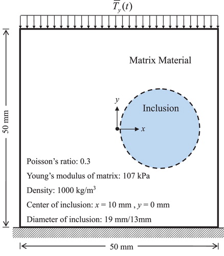
The FE model of the solid with the inclusion is formed with 50 × 50 bilinear elements and 2601 nodes. To avoid near zero energy modes, the spatial integration is performed by the 2 × 2 Gauss quadrature [16]. Finite elements that are completely included in the circles have the Young’s modulus of the inclusion. The total numbers of bilinear elements used to model the inclusions with the diameters of 19 and 13 mm are 256 and 114, respectively, and the corresponding area ratios of the inclusions to the whole solid become 10.24% and 4.56%. The FE dynamic analysis of the solid with the inclusion is performed for one second using the Newmark β-method [19] with a time increment of 10⁻⁴ s. The integration constants for the Newmark β-method, β = 1/2 and γ = 1/4, are adopted. Although damping is not considered in system identification, a small amount of damping is added for the dynamic analysis to suppress numerical noise in high frequency dynamic responses. The Rayleigh damping model [19], in which the damping ratios for the first and second modes are set to 0.01%, is utilized.

The system identification is performed based on an FE model with 10 × 10 bilinear elements and 121 nodal points unless otherwise stated. Each nodal point is an observation point, at which the dynamic displacements are measured. The measured displacements at the nodal points of the FE model are simulated by adding 5% proportional and absolute random noise to the displacements calculated by the dynamics analysis at the observation points [15]. (34) ${\overline{U}}_j(t)=U_j(t)+U_j(t){\eta }_j^p(t)+U^{ave}{\eta }_j^a(t)$(34) where $U_j(t)$ and $U^{ave}$ are the calculated displacement on the j-th DOF at the time t and the average of the absolute value of calculated displacement, respectively. ${\eta }_j^p$ and ${\eta }_j^a$ denote the uniformly distributed random numbers between ±5%, and are generated independently for all DOFs and all time steps. The target accuracy is set to 0.97 for both temporal and spatial filters, and the time-window size is selected as 1.5 times the period corresponding to the target frequency [15]. The convergence of the iteration for the T-S EEE is checked with the following criterion: (35) $\frac{{||{\mathbf{\text{E}}}_k-{\mathbf{\text{E}}}_{k-1}||}_2}{{||{\mathbf{\text{E}}}_k||}_2}\le {10}^{-2}$(35)

4.1. SI under free vibration

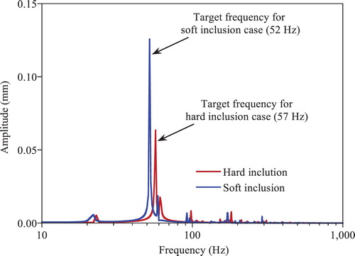
A compressive surface traction of 1 kN m^–2 is applied statically on the upper boundary of the solid, and is suddenly released to induce the free vibration of the solid. Identification results obtained by the conventional EEE with regularization are also presented. Figure 3 shows the FFT plots on the y-directional measured displacement at the centre of the solid with the hard and soft inclusion. Although several natural frequencies are identifiable in the figure, the dominant frequency is found at 52 Hz for the soft inclusion case and 57 Hz for the hard inclusion case, which are the second natural frequencies and selected as the target frequencies for the corresponding cases. The third and higher natural frequencies of solid are presented in the soft and hard inclusion cases, but these modes for both cases are not significant. The regularization factor is determined by the GMS [11] when the regularization scheme is employed in the SI. In forthcoming discussions, a colour scale is utilized in some figures to present identified Young’s moduli over the whole domain. The reference colours utilized in the colour scale are green, red and blue, which correspond to the reference Young’s moduli of 107 kPa (baseline value), 250 and 50 kPa, respectively. Intermediate values between two reference Young’s moduli are represented by a mixture of the corresponding reference colours.

Figure 3. FFT of measured y-directional displacement at the centre of the elastic solid with hard and soft inclusion under free vibration.

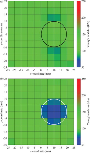
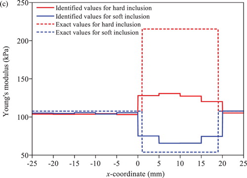
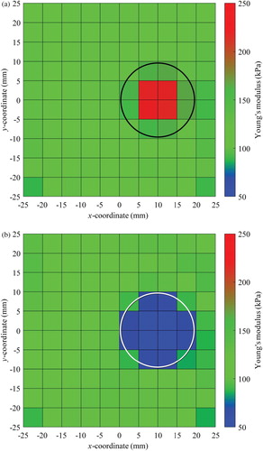
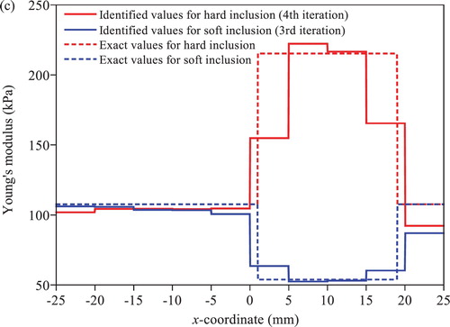
Figure 4 shows the identification results obtained by the conventional EEE with regularization. The 2nd-order Butterworth filter with the zero phase error filtering technique [17] is adopted to suppress high frequency noise in measured displacement, and the accelerations are calculated by the 2nd-order finite difference of the filtered displacements. The cutoff frequencies for the Butterworth filter are the same as those for the T-S filter. The filtered displacement and the numerically evaluated acceleration are utilized for the SI. The soft inclusion is clearly identified as illustrated in Figure 4(b). However, most information on the hard inclusion is lost in Figure 4(a). Figure 4(c) shows variations of the Young’s moduli along the 10 elements in the first layer above the centre line in x direction. As shown in the colour map, the Young’s modulus of the hard inclusion is slightly higher than the baseline value by about 20%, which make it difficult to identify the location, size and material property of the inclusion. The loss of information on a hard inclusion in SI is also observed in the study by Park et al. [11], in which the OEE with regularization is employed for a static problem.

Figure 4. Identified Young’s moduli under free vibration by the conventional EEE with regularization: (a) colour map for hard inclusion case (b) colour map for soft inclusion case (c) variation along the elements in the first layer above the centre line in x direction.

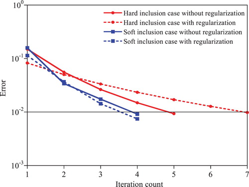
The T-S EEE accurately identifies not only the soft inclusion but also the hard inclusion as presented in Figures 5 and 6 regardless of the presence of regularization. As shown in the figures, the identification results are not affected much by the presence of regularization in the T-S EEE, which implies that the T-S filter sufficiently and efficiently eliminates noise in measured displacement and reconstructed acceleration to suppress the instability of SI problems caused by noise. Figure 7 shows the convergence rate of the T-S EEE. The solution of the soft inclusion case converges to the specified tolerance by 4 iterations regardless of the presence of regularization. The convergence rate becomes slightly slower for the hard inclusion case compared to the soft inclusion case. Moreover, the presence of regularization further slows down the convergence of the iteration procedure for the hard inclusion case. Based on the aforementioned discussions, it is concluded that the T-S EEE yields a very accurate and stable solution without the regularization scheme.

Figure 5. Identified Young’s moduli under free vibration by the T-S EEE for the hard inclusion case: (a) colour map of results without regularization (b) variation along the elements in the first layer above the centre line in x direction with/without regularization.

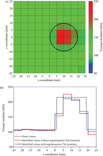
Figure 6. Identified Young’s moduli under free vibration by the T-S EEE for the soft inclusion case: (a) colour map of results without regularization (b) variation along the elements in the first layer above the centre line in x direction.

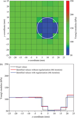
Figure 7. Convergence rates of the T-S EEE under free vibration.

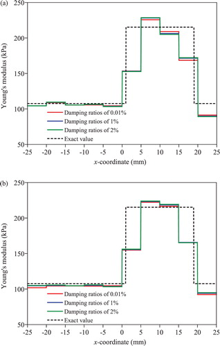
To demonstrate the general applicability of the T-S EEE, the system identification is performed for the different types of hard inclusions: (1) with a finer, 25 × 25 mesh; (2) with a smaller inclusion size; (3) with a lower Young’s modulus than the previous case; (4) with multiple inclusions and (5) with physically meaningful levels of damping ratios. The regularization scheme is not applied to these cases. Only the identification of the hard inclusion is presented because the conventional EEE with regularization also yields a good solution for the soft inclusion. Figure 8 shows the identification results for the 25 × 25 mesh. The location, size and the Young’ modulus for the hard inclusion are clearly identifiable in the colour map with a higher resolution. The proposed approach is tested for the hard inclusions with a diameter of 13 mm and with a Young’s modulus of 160.5 kPa, and the results are presented in Figures 9 and 10, respectively. These two cases are more difficult problems than the original problem because the difference between the solids with and without the inclusion is less noticeable. However, the T-S EEE yields good solutions for both cases without regularization. Figure 11 presents the identification results of the multiple inclusion case. A smaller circular inclusion with the Young’s modulus of 193.75 kPa and the diameter of 16 mm is added to the original hard inclusion case. The added inclusion is centred at x = −7.5 mm, y = −12.5 mm. As shown in the figure, the proposed T-S EEE yields accurate and stable results even for the multiple inclusion case. The T-S EEE is also tested for the numerically simulated displacement obtained using the Rayleigh damping model with damping ratios of 1% and 2% for the first two modes, and the results are shown in Figure 12(a). No noticeable difference in the identification results is found for the measured displacements obtained for the higher damping ratios even though the damping term is not included in the T-S EEE.

Figure 8. Identified Young’s moduli under free vibration by the T-S EEE without regularization for the hard inclusion case with 25 × 25 mesh layout: (a) colour map (b) variation along the elements in the centre layer in x direction.

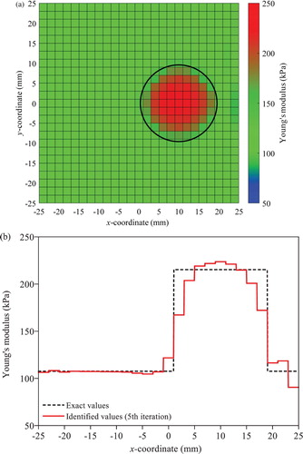
Figure 9. Identified Young’s moduli under free vibration by the T-S EEE without regulation for the hard inclusion with diameter of 13 mm: (a) colour map (b) variation along the elements in the first layer above the centre line in x direction.

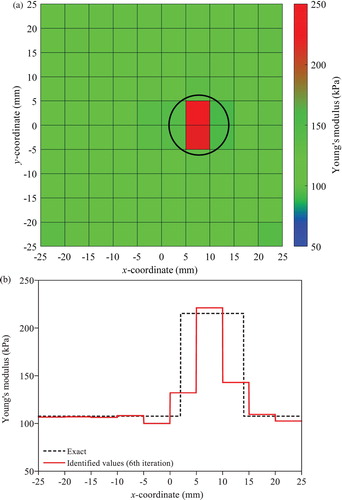
Figure 10. Identified Young’s moduli under free vibration by the T-S EEE without regulation for the hard inclusion with Young’s modulus of 160.5 kPa: (a) colour map (b) variation along the elements in the first layer above the centre line in x direction.

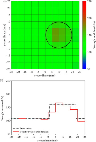
Figure 11. Identified Young’s moduli under free vibration by the T-S EEE without regularization for the multi inclusion case: (a) colour map (b) variation along the elements in the first layer above the centre line in x direction (c) variation along the elements in the third layer above the bottom line in x direction.

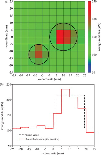
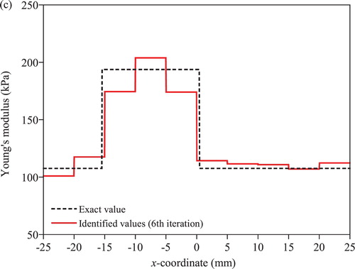
Figure 12. Identified Young’s moduli along the elements in the first layer above the centre line in x direction for three different damping ratios: (a) free vibration and (b) forced vibration.

It is worthwhile at this point to discuss the differences in the stabilization effect provided by the regularization scheme and the proposed approach. The stabilization effect of the regularization scheme is explained using the eigenvalue decomposition (EVD) of the integral term of the first equation in Equation (17). As is well known, the EVD decomposes a matrix into the product of the eigenvectors and the eigenvalues, and leads to the solution of Equation (16) as follows: (36) $\mathbf{\text{E}}=-{\overline{\mathbf{\text{Q}}}}^{-1}\overline{\mathbf{\text{Z}}}=-{\left(\sum _i{\mathit{\varphi }}_i{\mathrm{\Lambda }}_i{\mathit{\varphi }}_i^T+{\lambda }_E^2\mathbf{\text{I}}\right)}^{-1}\overline{\mathbf{\text{Z}}}=-\sum _i\frac{{\mathit{\varphi }}_i^T\overline{\mathbf{\text{Z}}}}{{\mathrm{\Lambda }}_i+{\lambda }_E^2}{\mathit{\varphi }}_i$(36) where Λ_i and φ_i are the i-th eigenvalue and eigenvector of the integral term of the first equation in Equation (17), respectively. The eigenvectors are orthogonal to each other. In case the regularization term is not included in the EEE, i.e. λ_E= 0, the solution of an SI problem is expressed as a linear combination of the eigenvectors, of which the coefficients are calculated as the dot product between $\overline{\mathbf{\text{Z}}}$ and the eigenvectors divided by the corresponding eigenvalues. If measured data contain noise, the eigenvectors and $\overline{\mathbf{\text{Z}}}$ are polluted by the noise. As a consequence, the noise in the coefficients corresponding to small eigenvalues is amplified and governs the whole solution of the EEE. Provided that, however, the regularization factor is properly selected, the denominators in Equation (36) corresponding to smaller eigenvalues increase significantly, which prevents the amplification of noise. However, physical information associated with the eigenvectors corresponding to small eigenvalues is also lost, and thus identification results may lose physical significance. As the information on hard inclusions is associated with eigenvectors corresponding to small eigenvalues, most information on hard inclusions in measured data is lost, and thus the conventional EEE with regularization is unable to identify the hard inclusions accurately. On the other hand, the T-S EEE does not alter the system matrix, and preserves the system characteristics of a given problem. Rather, noise components in measured displacement and reconstructed acceleration themselves are suppressed by the T-S filter, which provides a stabilization effect on the solution of an SI problem. Therefore, every information on the eigenvector is preserved in the identification of both the soft and hard inclusions.

To confirm the robustness of the proposed T-S EEE against random noise, the Young’s modulus of each element obtained with and without added random noise is compared in Figure 13(a) for the hard inclusion case. The elements in the four blue circles correspond to those in the two middle layers of the inclusion in Figure 5(a). The four elements above and below the two middle layers are indicated with two green circles. As shown in the figure, the identified Young’s moduli are virtually identical for the noise-free and noise-added measurement. This is because the T-S filter employed in this study almost completely filters out random noise, and thus noise in measurement does not affect the identification results. The deviations of the identified Young’s moduli from the exact solution are solely caused by the modelling and discretization error of the FE model, which cannot be eliminated by the T-S filter. Here, the modelling error implies that the exact circular shape of the inclusion cannot be presented by the FE mesh used in the SI. Consequently, it is believed that the T-S EEE would be insensitive to random noise in measurement, and yield stable and accurate solutions as long as the noise level in measurement is not unreasonably high.

Figure 13. Effect of noise in measusrement (a) identified Young’s modulus of each element with and without noise; (b) Mean and standard deviation of identified Young’s modulus of each element by 100 Monte-Carlo Trials.

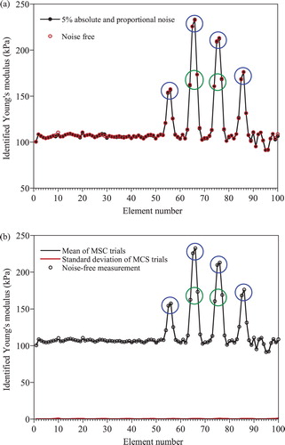
The insensitiveness of the T-S EEE to noise is demonstrated through the Monte-Carlo simulation with 100 trials. A distinct noise set of 5% proportional and absolute random noise is generated for each Monte-Carlo trial by the procedure in Equation (34). Figure 13(b) presents the mean and standard deviation of the identified Young’s modulus of each element along with the results by the noise-free measurement in Figure 13(a). The mean values of the identified Young’s moduli of all elements coincide with those by the noise-free measurement, and their standard deviations are practically zero. The coefficients of variation, which are the ratios of the standard deviations to the means, range between 0.2% and 1.2% for all elements. These results demonstrate that identification results by the T-S EEE are scarcely affected by random noise in the measurement.

4.2. SI under forced vibration

The proposed T-S EEE is tested for a forced-vibration condition. The regularization scheme is not considered in this example because the regularization scheme does not improve the solution of the T-S EEE as shown in the previous examples. The solid is excited by the following y-directional surface traction applied on the upper boundary. (37) ${\overline{T}}_y(t)=\{\begin{array}{l}2t[\sin (130\pi t)+\sin (190\pi t)+\sin (250\pi t)+\sin (300\pi t)]\text{kN/}{\text{m}}^2\text{ for }t\le 0.1s\\ 0.2[\sin (130\pi t)+\sin (190\pi t)+\sin (250\pi t)+\sin (300\pi t)]\text{kN/}{\text{m}}^{\text{2}}\text{ for }t>0.1s\end{array}$(37) The excitation traction gradually increases from 0 at $t=0\text{s}$ to its full amplitude at $t=0.1\text{ s}$. The excitation frequencies of the traction are 65, 95, 125 and 150 Hz. The random noise is generated as described earlier in this section, and added to the dynamic displacement calculated by the FE model. The measurement duration is set to one second.

Figure 14 shows the FFT plots of the y-directional displacement measured at the centre of the solid with the soft and hard inclusion. All excitation frequencies are clearly observed for the hard inclusion case, while only two lower excitation frequencies are identifiable in the soft inclusion case. The first natural mode of the solid is not triggered and the second natural mode is clearly observable in the plot. The target frequency of the T-S filter is selected as 95 Hz as the frequency contents above 95 Hz are negligibly small. The identified Young’s moduli of the hard and soft inclusion case using the T-S EEE are shown in Figure 15. The solutions of hard and soft inclusion case converge at the 4th and 3rd iteration, respectively, and the inclusions are well identified as the free-vibration condition. With this example, it is concluded that the T-S EEE is applicable to SI problems with various types of excitation sources. Figure 12(b) presents the identification results for the measured displacement obtained for the higher damping ratios used for the free vibration case in the previous section. As with the free vibration case, the T-S EEE yields a stable and accurate solution.

Figure 14. FFT of the y-directional displacement measured at the centre of the elastic solid with hard and soft inclusion under forced vibration.

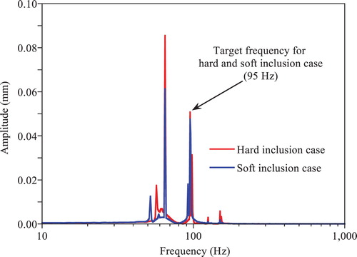
Figure 15. Identified Young’s moduli under forced vibration by the TS filter without regularization: (a) colour map for hard inclusion case (b) colour map for soft inclusion case (c) variation along the elements in the first layer above the centre line in x direction.

5. Summary and conclusion

A new class of an SI scheme based on the EEE is proposed using the T-S filter. The stabilization effect of the proposed approach is obtained by eliminating the noise components in measured displacement and reconstructed acceleration through the T-S filter. As the proposed approach uses de-noised dynamic responses without sacrificing physically meaningful information in measured data, every piece of system information in the measured data is utilized, and a more precise estimation of system parameters becomes possible. On the other hand, the conventional EEE with the regularization scheme sometimes suppresses not only noise in measurement but also useful information on a system, which leads to inaccurate identification results. The proposed approach becomes a nonlinear problem because the T-S filter is a function of the Young’s modulus of a given elastic solid. The successive substitution method is adopted to solve the nonlinear system equation. The detailed expression of the sensitivity of the T-S filter with respect to the Young’s modulus is derived by the direct differentiation method.

The validity and efficiency of the T-S EEE are demonstrated through numerical simulation studies on the identification of various types of inclusions in a finite elastic body. The conventional EEE with the regularization scheme is also tested. The proposed approach yields very accurate solutions regardless of the size, Young’s modulus of an inclusion, mesh layouts for the SI and excitation types. Meanwhile, the conventional EEE with the regularization scheme fails to identify the hard inclusion clearly. Detailed discussions on different characteristics of the stabilization effect provided by the two methods are presented. The proposed approach may provide a powerful engineering tool for various types of SI problems, especially when a problem is defined in a relatively small domain and displacement can be measured densely in the spatial domain.

Disclosure statement

No potential conflict of interest was reported by the author(s).

References

- Park EY, Maniatty AM. Shear modulus reconstruction in dynamic elastography: time harmonic case. Phys Med Biol. 2006;51:3697–3721. doi: 10.1088/0031-9155/51/15/007
- Park EY, Maniatty AM. Finite element formulation for shear modulus reconstruction in transient elastography. Inverse Probl Sci Eng. 2009;17:605–626. doi: 10.1080/17415970802358371
- Hjelmstad KD, Banan MR, Banan MR. Time-domain parameter estimation algorithm for structures. I: computational aspects. J Eng Mech. 1995;121(3):424–434. doi: 10.1061/(ASCE)0733-9399(1995)121:3(424)
- Banan MR, Hjelmstad KD. Time-domain parameter estimation algorithm for structures II: numerical simulation studies. J Eng Mech. 1995;121(3):435–447. doi: 10.1061/(ASCE)0733-9399(1995)121:3(435)
- Liu J, Meng X, Zhang D, et al. An Efficient method to reduce Ill-posedness for structural dynamic load identification. Mech Syst Signal Process. 2017;95:273–285. doi: 10.1016/j.ymssp.2017.03.039
- Ghafory-Ashtiany M, Ghasemi M. System identification method by using inverse solution of equations of motion in frequency domain. J Vib Control. 2012;19(11):1633–1645. doi: 10.1177/1077546312448079
- Huang C-H. A non-linear inverse vibration problem of estimating the time-dependent stiffness coefficients by conjugate gradient method. Int J Numer Meth Engng. 2001;50:1545–1558. doi: 10.1002/nme.83
- Li J, Law SS. Damage identification of a target substructure with moving load excitation. Mech Syst Signal Process. 2012;30:78–90. doi: 10.1016/j.ymssp.2012.02.002
- Vegel CR. Optimal choice of a truncation level for the truncated SVD solution of linear first kind integral equations when data are noisy. SIAM J Numer Anal. 1986;23(1):109–117. doi: 10.1137/0723007
- Lee HS, Kim YH, Park CJ, et al. A new spatial regularization scheme for the identification of geometric shapes of inclusions in finite bodies. Int J Numer Meth Engng. 1999;46(7):973–992. doi: 10.1002/(SICI)1097-0207(19991110)46:7<973::AID-NME730>3.0.CO;2-Q
- Park HW, Shin SB, Lee HS. Determination of an optimal regularization factor in system identification with Tikhonov function for linear elastic continua. Int J Numer Meth Engng. 2001;51(10):1211–1230. doi: 10.1002/nme.219
- Park HW, Park MW, Ahn BK, et al. 1-norm-based regularization scheme for system identification of structures with discontinuous system parameters. Int J Numer Meth Engng. 2007;69(3):504–523. doi: 10.1002/nme.1778
- Bui HD. Inverse problems in the mechanics of materials: an introduction. Boca Raton (FL): CRC Press; 1994.
- Hansen PC. Rank-deficient and discrete ill-posed problems: numerical aspects of linear inversion. Philadelphia: SIAM; 1998.
- Park K-Y, Lee HS. Design of de-noising FEM-FIR filters for the evaluation of temporal and spatial derivatives of measured displacement in elastic solids. Mech Syst Signal Process. 2019;120:524–539. doi: 10.1016/j.ymssp.2018.10.034
- Hughes TJR. The finite element method: linear static and dynamic finite element analysis. Englewood Cliffs (NJ): Prentice-Hall; 1987.
- Hamming RW. Digital filters. 3rd ed. Englewood Cliffs (NJ): Prentice-Hall; 1989.
- Lee HS, Hong YH, Park HW. Design of an FIR filter for the displacement reconstruction using measured acceleration in low-frequency dominant structures. Int J Numer Methods Eng. 2010;82:403–434.
- Chopra AK. Dynamics of structures: theory and applications to earthquake engineering. 2nd ed. Upper Saddle River (NJ): Prentice-Hall; 2001.