A total variation regularization method for an inverse problem of recovering an unknown diffusion coefficient in a parabolic equation

Abstract

This paper studies an inverse problem of recovering an unknown diffusion coefficient in a parabolic equation. We adopt a total variation regularization method to deal with the ill-posedness. This method has the advantage to solve problems that the solution is non-smooth or discontinuous. By transforming the problem into an optimal control problem, we derive a necessary condition of the control functional. Through some prior estimates of the direct problem, the uniqueness and stability of the minimizer are obtained. In the numerical part, a Gauss–Jacobi iteration scheme is used to deal with the non-linear term. Some numerical examples are presented to illustrate the performance of the proposed algorithm.

Keywords:

• Parabolic equation
• total variation
• inverse problem
• optimal control
• regularization

2010 Mathematics Subject Classifications:

• 35R30
• 49J20

1. Introduction

The mathematical models describing the diffusion process are of great importance in many scientific fields, such as heat conduction, diffusion, groundwater flow, oil reservoir simulation, etc. The aim of the direct problem is to determine the diffusion field according to the system parameters. However, in many practical situations, the diffusion parameters may not be known. The purpose of the inverse problem is to reconstruct these parameters from the observation data of the diffusion field. In this paper, we consider a simple model based on the following parabolic equation (1) $\begin{array}{ll}{u}_t-(k(x)u_x{)}_x=f(x,t),& (x,t)\in D_T,\\ u(x,0)=\phi (x),& x\in [0,l],\\ u(0,t)=u(l,t)=0,& t\in [0,T],\end{array}$(1) where $D_T=(0,l)\times (0,T]$, $f\in L^2(D_T)$ and $\phi \in L^2[0,l]$ are two given functions, $k(x)$ is an unknown diffusion coefficient. Assume that the final observation data, i.e. (2) $u(x,T)=s(x),x\in [0,l],$(2) is given. The goal of the inverse problem is to reconstruct $k(x)$ in Equation (1(1) $\begin{array}{ll}{u}_t-(k(x)u_x{)}_x=f(x,t),& (x,t)\in D_T,\\ u(x,0)=\phi (x),& x\in [0,l],\\ u(0,t)=u(l,t)=0,& t\in [0,T],\end{array}$(1) ). The mathematical model (1(1) $\begin{array}{ll}{u}_t-(k(x)u_x{)}_x=f(x,t),& (x,t)\in D_T,\\ u(x,0)=\phi (x),& x\in [0,l],\\ u(0,t)=u(l,t)=0,& t\in [0,T],\end{array}$(1) ) arises in many engineering and physical settings, for example, the heat conduction in a rod. Being different from the corresponding direct problem, the inverse problem is ill posed [1]. In many practical applications, the observation data $s(x)$ in (2(2) $u(x,T)=s(x),x\in [0,l],$(2) ) is obtained by measurements. A small noise in $s(x)$ may cause a big change in the reconstructions of $k(x)$, which may lead to a meaningless result [2,3].

There has been many works related to this inverse problem. In [4], a semigroup method is used to analyse the existence of the solution of the inverse problem and the local representation of the unknown diffusion coefficient is obtained at the end points. In [5] the uniqueness and conditional stability of the inverse problem are studied by transforming the problem into a non-linear operator equation. The numerical solution is obtained by an iteratively regularized Gauss–Newton method. In [6] an optimization scheme with both $H^1$-regularization and BV-regularization are discussed. The existence and convergence of the approximate solution to the problem is obtained in the framework of finite element analysis and the Armijo algorithm is applied for the numerical solution. In [7] the problem is transformed into an optimal control problem, and the uniqueness and stability of the control functional are proved. The stable numerical solution is obtained by the gradient iteration method. There are also some other works, see [8–16] and the references therein.

The optimization method is a powerful tool for dealing with the ill-posed problems [17–20]. The basic idea is to restrict the problem to some compact set, and then get the solution by minimizing the following functional [21] $\underset{x}{min}\Vert Fx-y{\Vert }^2+\lambda \hat{J}(x),x\in \mathcal{X},y\in \mathcal{Y},$ where $F:\mathcal{X}\to \mathcal{Y}$ is a forward map, $\lambda >0$ is a regularization parameter and $\hat{J}(x)$ is a penalty term. According to the prior knowledge of the inversion solution, $\hat{J}(x)$ can be chosen differently. The well-known Tikhonov regularization method [22] is to use the $L^2$ norm as a penalty term, and this method usually works well for continuous models. However, in many practical applications, the solution of the problem may not be continuous. For example, in image processing, a common problem of Tikhonov regularization is that it will smooth out the sharp edges of an image and can not preserve the detailed information very well [23]. In [24] a total variation regularization method was proposed by Rudin et al. and good results are achieved in the field of image processing. The definition of total variation [25,26] can be expressed as $TV(k):={\int }_{\mathrm{\Omega }}|\mathrm{\nabla }k|\mathrm{d}x=sup\{{\int }_{\mathrm{\Omega }}k\mathrm{div}(v)\mathrm{d}x:v\in C_0^1(\mathrm{\Omega }),|v(x)|⩽1\}.$ The total variation of k is also known as the bounded variation of k. The space of all functions in $L^1(\mathrm{\Omega })$ with bounded variation is denoted by $BV(\mathrm{\Omega })=\{k\in L^1(\mathrm{\Omega }):{\int }_{\mathrm{\Omega }}|\mathrm{\nabla }k|\mathrm{d}x<\mathrm{\infty }\},$ and the corresponding BV-norm is given by $\Vert k{\Vert }_{BV}=\Vert k{\Vert }_{L^1}+{\int }_{\mathrm{\Omega }}|\mathrm{\nabla }k|\mathrm{d}x.$ It can be proved that $BV(\mathrm{\Omega })$ is complete under the BV-norm and thus a Banach space. In addition, if Ω is a bounded open set with Lipschitz boundary in $R^n(n⩾1)$, then $W^{1,1}⊊BV$ (see [27] for more details). Total variation regularization is one of the most effective tools to solve problems when the solution is non-smooth or discontinuous.

Compared with the intensive study of total variation regularization method in image processing, the applications of this method for reconstructing an unknown coefficient of partial differential equations are much less, see [28–34]. There are also some difficulties for total variation regularization method both theoretically and numerically [35,36]. For example, the non-differentiability of the TV-term can bring great difficulties to theoretical analysis; in numerical calculation, its nonlinearity and degeneracy can also make the algorithm more complex. In this paper, from a point of view of theoretical analysis, we adopt an optimal control framework to discuss this problem. By introducing a polished TV-term, we derive a necessary condition of the control functional. The necessary condition which is a variational inequality with a coupled system of a parabolic equation. Being different from the previous work in [7], the variational inequality in this paper includes a non-linear term. In order to get the uniqueness and stability results, we also need an additional condition (3) $max|\mathrm{\nabla }k|⩽\kappa ,$(3) where κ is a positive constant. In the numerical part, we modify this necessary condition into an equality form and adopt a Gauss–Jacobi iteration scheme to deal with the nonlinear term. The numerical results show that this modification is effective and can reconstruct the non-smooth solutions very well.

The organization of this paper is as follows: Section 2 transforms the problem into an optimal control problem and derives a necessary condition for the control functional. Section 3 studies the well-posedness of the optimal control problem based on the necessary condition. Section 4 discretizes the system and give a numerical algorithm. Section 5 presents some numerical examples to illustrate the effectiveness of the algorithm.

2. Optimal control problem

It is well known that the original problem is ill-posed and cannot be solved directly. The most applicable method for solving this problem is the Tikhonov regularization method. However, Tikhonov regularization method often requires some smoothness of the solution. In many practical applications, the solution of the problem may not always be continuous. To overcome this difficulty, we consider the following total variation regularization-based optimal control problem.

Problem P. Define an admissible domain (4) $\mathcal{K}:=\{k\in L^1(0,l):\Vert k{\Vert }_{BV}<\mathrm{\infty }\text{ and }0<{\zeta }_1⩽k(x)⩽{\zeta }_2,\text{ a.e. in }(0,l)\},$(4) where ${\zeta }_1,{\zeta }_2$ are two given positive constants. Assume that the observation data $s(x)$ in (2(2) $u(x,T)=s(x),x\in [0,l],$(2) ) satisfies the following condition (5) $s(x)\in L^2[0,l].$(5) The optimal control problem in this study is to find $k^{\ast }\in \mathcal{K}$ such that (6) $\begin{array}{rl}J(k^{\ast })& =\underset{k\in \mathcal{K}}{min}J(k),\end{array}$(6) (7) $\begin{array}{rl}J(k)& =\frac{1}{2}{\int }_0^l|u(x,T;k)-s(x){|}^2\mathrm{d}x+\lambda \hat{J}(k),\end{array}$(7) where $\hat{J}(k)={\int }_0^l|k^{\mathrm{\prime }}|\mathrm{d}x$ (in order to avoid the potential misleading of the divergence notation, we use the notation $|k^{\mathrm{\prime }}|$ instead of $|\mathrm{\nabla }k|$ in the TV-penalty term, because our problem is one-dimensional), $u(x,T;k)$ is the solution of Equation (1(1) $\begin{array}{ll}{u}_t-(k(x)u_x{)}_x=f(x,t),& (x,t)\in D_T,\\ u(x,0)=\phi (x),& x\in [0,l],\\ u(0,t)=u(l,t)=0,& t\in [0,T],\end{array}$(1) ) corresponding to $k(x)$ and $\lambda >0$ is a regularization parameter.

Following [36], we modify the penalty term $\hat{J}(k)$ as (8) ${\hat{J}}_{\beta }(k)={\int }_0^l\sqrt{|k^{\mathrm{\prime }}{|}^2+\beta }\mathrm{d}x,$(8) where β is a small positive parameter and in this paper it is taken as $\beta ={10}^{-4}$. This modification can provide certain advantages in computation, such as differentiability of ${\hat{J}}_{\beta }$ when $k^{\mathrm{\prime }}(x)=0$. According to (8(8) ${\hat{J}}_{\beta }(k)={\int }_0^l\sqrt{|k^{\mathrm{\prime }}{|}^2+\beta }\mathrm{d}x,$(8) ) the optimal control problem (6(6) $\begin{array}{rl}J(k^{\ast })& =\underset{k\in \mathcal{K}}{min}J(k),\end{array}$(6) ) and (7(7) $\begin{array}{rl}J(k)& =\frac{1}{2}{\int }_0^l|u(x,T;k)-s(x){|}^2\mathrm{d}x+\lambda \hat{J}(k),\end{array}$(7) ) can be approximated by (9) $\begin{array}{rl}J(k^{\ast })& =\underset{k\in \mathcal{K}}{min}J(k),\end{array}$(9) (10) $\begin{array}{rl}J(k)& =\frac{1}{2}{\int }_0^l|u(x,T;k)-s(x){|}^2\mathrm{d}x+\lambda {\hat{J}}_{\beta }(k).\end{array}$(10)

Definition 2.1

cf.[37]

A function $u\in L^2((0,T),H_0^1(0,l))$, with $u_t\in L^2((0,T),H^{-1}(0,l))$ is called the a weak solution of Equation (1(1) $\begin{array}{ll}{u}_t-(k(x)u_x{)}_x=f(x,t),& (x,t)\in D_T,\\ u(x,0)=\phi (x),& x\in [0,l],\\ u(0,t)=u(l,t)=0,& t\in [0,T],\end{array}$(1) ), if (11) ${\int }_0^l{u}_t\varphi \mathrm{d}x+{\int }_0^{l}k{u}_x{\varphi }_x\mathrm{d}x={\int }_0^{l}f\varphi \mathrm{d}x,$(11) for any test function $\varphi (x)\in H_0^1(0,l)$ and a.e. time $0⩽t⩽T$ and $u(x,0)=\phi (x).$

Lemma 2.2

cf.[38,39]

For Equation (1(1) $\begin{array}{ll}{u}_t-(k(x)u_x{)}_x=f(x,t),& (x,t)\in D_T,\\ u(x,0)=\phi (x),& x\in [0,l],\\ u(0,t)=u(l,t)=0,& t\in [0,T],\end{array}$(1) ) we have the following estimate (12) $\underset{0⩽t⩽T}{max}{\int }_0^l{u}^2\mathrm{d}x+{\int }_0^T{\int }_0^l|u_x{|}^2\mathrm{d}x\mathrm{d}t⩽C[{\int }_0^l{\phi }^2\mathrm{d}x+{\int }_0^T{\int }_0^l{f}^2\mathrm{d}x\mathrm{d}t],$(12) where C is independent of ϕ and f.

Now, we are going to prove the existence of minimizers of problem P. In order to get this result, we first give the continuous property of $J(k)$ by the following lemma.

Lemma 2.3

Assume that $\{k_n,n=1,2,\dots \}\subset \mathcal{K},$ $k{}^{\ast }\in \mathcal{K},$ and $\Vert k_n-k{}^{\ast }{\Vert }_{L^1[0,l]}\to 0,$ as $n\to \mathrm{\infty },$ then we have (13) $\underset{n\to \mathrm{\infty }}{lim}{\int }_0^l|u(x,T;k_n)-s(x){|}^2\mathrm{d}x={\int }_0^l|u(x,T;k{}^{\ast })-s(x){|}^2\mathrm{d}x.$(13)

Proof.

Let $k=k_n$ and choosing the test function φ in (11(11) ${\int }_0^l{u}_t\varphi \mathrm{d}x+{\int }_0^{l}k{u}_x{\varphi }_x\mathrm{d}x={\int }_0^{l}f\varphi \mathrm{d}x,$(11) ) as $u(k_n)(x,\cdot )$ (for abbreviation, we denote it by $u(k_n)$), which depends on x, we obtain ${\int }_0^t{\int }_0^l{u}_t(k_n)u(k_n)\mathrm{d}x\mathrm{d}t+{\int }_0^t{\int }_0^l{k}_n|u_x(k_n){|}^2\mathrm{d}x\mathrm{d}t={\int }_0^t{\int }_0^{l}fu(k_n)\mathrm{d}x\mathrm{d}t.$ According to Gronwall's inequality and Cauchy's inequality, we have (14) ${\int }_0^l|u(k_n){|}^2\mathrm{d}x+{\int }_0^t{\int }_0^l{k}_n|u_x(k_n){|}^2\mathrm{d}x\mathrm{d}t⩽C{\int }_0^l{\phi }^2\mathrm{d}x+C{\int }_0^t{\int }_0^l{f}^2\mathrm{d}x\mathrm{d}t.$(14) From (14(14) ${\int }_0^l|u(k_n){|}^2\mathrm{d}x+{\int }_0^t{\int }_0^l{k}_n|u_x(k_n){|}^2\mathrm{d}x\mathrm{d}t⩽C{\int }_0^l{\phi }^2\mathrm{d}x+C{\int }_0^t{\int }_0^l{f}^2\mathrm{d}x\mathrm{d}t.$(14) ), we know that $\Vert u(k_n){\Vert }_{L^2((0,T);H_0^1(0,l))}$ is uniformly bounded for all $k_n\in \mathcal{K}$. Therefore, we can extract a subsequence of $u(k_n)$, still denoted by $u(k_n)$, such that (15) $u(x,t;k_n)\rightharpoonup u^{\ast }(x,t;k)\in L^2((0,T);H_0^1(0,l)).$(15) Now we will show that $u^{\ast }=u(k{}^{\ast })$. Multiplying both sides of (11(11) ${\int }_0^l{u}_t\varphi \mathrm{d}x+{\int }_0^{l}k{u}_x{\varphi }_x\mathrm{d}x={\int }_0^{l}f\varphi \mathrm{d}x,$(11) ) by a function $\xi (t)\in C^1[0,T]$ with $\xi (T)=0$ and taking $k=k_n$, then we have ${\int }_0^T{\int }_0^l{u}_t(k_n)\varphi \xi (t)\mathrm{d}x\mathrm{d}t+{\int }_0^T{\int }_0^l{k}_n{u}_x(k_n){\varphi }_x\xi (t)\mathrm{d}x\mathrm{d}t={\int }_0^T{\int }_0^{l}f\varphi \xi (t)\mathrm{d}x\mathrm{d}t.$ Integrating by parts, we obtain (16) $\begin{array}{rl}{\int }_0^l\phi (x)\varphi \xi (0)\mathrm{d}x& =-{\int }_0^T{\int }_0^{l}u(k_n)\varphi {\xi }_t(t)\mathrm{d}x\mathrm{d}t+{\int }_0^T{\int }_0^l(k_n-k{}^{\ast })u_x(k_n){\varphi }_x\xi (t)\mathrm{d}x\mathrm{d}t\\ & +{\int }_0^T{\int }_0^{l}k{}^{\ast }{u}_x(k_n){\varphi }_x\xi (t)\mathrm{d}x\mathrm{d}t-{\int }_0^T{\int }_0^{l}f\varphi \xi (t)\mathrm{d}x\mathrm{d}t.\end{array}$(16) From (15(15) $u(x,t;k_n)\rightharpoonup u^{\ast }(x,t;k)\in L^2((0,T);H_0^1(0,l)).$(15) ) and taking $n\to \mathrm{\infty }$ in (16(16) $\begin{array}{rl}{\int }_0^l\phi (x)\varphi \xi (0)\mathrm{d}x& =-{\int }_0^T{\int }_0^{l}u(k_n)\varphi {\xi }_t(t)\mathrm{d}x\mathrm{d}t+{\int }_0^T{\int }_0^l(k_n-k{}^{\ast })u_x(k_n){\varphi }_x\xi (t)\mathrm{d}x\mathrm{d}t\\ & +{\int }_0^T{\int }_0^{l}k{}^{\ast }{u}_x(k_n){\varphi }_x\xi (t)\mathrm{d}x\mathrm{d}t-{\int }_0^T{\int }_0^{l}f\varphi \xi (t)\mathrm{d}x\mathrm{d}t.\end{array}$(16) ), we deduce (17) ${\int }_0^l\phi (x)\varphi \xi (0)\mathrm{d}x=-{\int }_0^T{\int }_0^l{u}^{\ast }\varphi {\xi }_t(t)-k{}^{\ast }{u}_x^{\ast }{\varphi }_x\xi (t)\mathrm{d}x\mathrm{d}t-{\int }_0^T{\int }_0^{l}f\varphi \xi (t)\mathrm{d}x\mathrm{d}t.$(17) Notice that (17(17) ${\int }_0^l\phi (x)\varphi \xi (0)\mathrm{d}x=-{\int }_0^T{\int }_0^l{u}^{\ast }\varphi {\xi }_t(t)-k{}^{\ast }{u}_x^{\ast }{\varphi }_x\xi (t)\mathrm{d}x\mathrm{d}t-{\int }_0^T{\int }_0^{l}f\varphi \xi (t)\mathrm{d}x\mathrm{d}t.$(17) ) is valid for any $\xi (t)\in C^1[0,T]$ with $\xi (T)=0$, so we have ${\int }_0^l{u}_t^{\ast }\varphi \mathrm{d}x+{\int }_0^{l}k{}^{\ast }{u}_x^{\ast }{\varphi }_x\mathrm{d}x={\int }_0^{l}f\varphi \mathrm{d}x,\mathrm{\forall }\varphi \in H_0^1(0,l),$ and $u^{\ast }(x,0)=\phi (x)$. Hence, $u^{\ast }=u(k{}^{\ast })$ by the definition of $u(k)$.

Through the weak convergence of $u(k_n)\rightharpoonup u(k^{\ast })$, next we will show the convergence of $u(k_n)$ in the sense of $L^2$ topology. By taking $k=k_n$ and $\varphi =u(k_n)-s$, then from (11(11) ${\int }_0^l{u}_t\varphi \mathrm{d}x+{\int }_0^{l}k{u}_x{\varphi }_x\mathrm{d}x={\int }_0^{l}f\varphi \mathrm{d}x,$(11) ) we have (18) $\begin{array}{rl}& \frac{1}{2}\frac{\mathrm{d}}{\mathrm{d}t}\Vert u(k_n)-s{\Vert }_{L^2(0,l)}^2+{\int }_0^l{k}_n|(u(k_n)-s{)}_x{|}^2\mathrm{d}x\\ & ={\int }_0^{l}f(u(k_n)-s)\mathrm{d}x-{\int }_0^l{k}_n{s}_x(u(k_n)-s{)}_x\mathrm{d}x.\end{array}$(18) A similar discussion for $u(k{}^{\ast })$, we have (19) $\begin{array}{rl}& \frac{1}{2}\frac{\mathrm{d}}{\mathrm{d}t}\Vert u(k{}^{\ast })-s{\Vert }_{L^2(0,l)}^2+{\int }_0^{l}k{}^{\ast }|(u(k{}^{\ast })-s{)}_x{|}^2\mathrm{d}x\\ & ={\int }_0^{l}f(u(k{}^{\ast })-s)\mathrm{d}x-{\int }_0^{l}k{}^{\ast }{s}_x(u(k{}^{\ast })-s{)}_x\mathrm{d}x.\end{array}$(19) Combining (18(18) $\begin{array}{rl}& \frac{1}{2}\frac{\mathrm{d}}{\mathrm{d}t}\Vert u(k_n)-s{\Vert }_{L^2(0,l)}^2+{\int }_0^l{k}_n|(u(k_n)-s{)}_x{|}^2\mathrm{d}x\\ & ={\int }_0^{l}f(u(k_n)-s)\mathrm{d}x-{\int }_0^l{k}_n{s}_x(u(k_n)-s{)}_x\mathrm{d}x.\end{array}$(18) ) and (19(19) $\begin{array}{rl}& \frac{1}{2}\frac{\mathrm{d}}{\mathrm{d}t}\Vert u(k{}^{\ast })-s{\Vert }_{L^2(0,l)}^2+{\int }_0^{l}k{}^{\ast }|(u(k{}^{\ast })-s{)}_x{|}^2\mathrm{d}x\\ & ={\int }_0^{l}f(u(k{}^{\ast })-s)\mathrm{d}x-{\int }_0^{l}k{}^{\ast }{s}_x(u(k{}^{\ast })-s{)}_x\mathrm{d}x.\end{array}$(19) ), we obtain (20) $\begin{array}{rl}& \frac{1}{2}\frac{\mathrm{d}}{\mathrm{d}t}\Vert u(k_n)-u(k{}^{\ast }){\Vert }_{L^2(0,l)}^2+{\int }_0^l{k}_n|(u(k_n)-s{)}_x{|}^2\mathrm{d}x-{\int }_0^{l}k{}^{\ast }|(u(k{}^{\ast })-s{)}_x{|}^2\mathrm{d}x\\ & ={\int }_0^{l}f(u(k_n)-u(k{}^{\ast }))\mathrm{d}x+{\int }_0^{l}k{}^{\ast }{s}_x(u(k{}^{\ast })-u(k_n){)}_x\mathrm{d}x\\ & +{\int }_0^l(k{}^{\ast }-k_n)s_x(u(k_n)-s{)}_x\mathrm{d}x-{\int }_0^l\frac{\mathrm{d}}{\mathrm{d}t}[(u(k{}^{\ast })-s)(u(k_n)-u(k{}^{\ast }))]\mathrm{d}x.\end{array}$(20) Furthermore, by using equation (11(11) ${\int }_0^l{u}_t\varphi \mathrm{d}x+{\int }_0^{l}k{u}_x{\varphi }_x\mathrm{d}x={\int }_0^{l}f\varphi \mathrm{d}x,$(11) ) for $u(k_n)$ and $u(k{}^{\ast })$, we deduce (21) $\begin{array}{rl}& {\int }_0^l\frac{\mathrm{d}}{\mathrm{d}t}[(u(k{}^{\ast })-s)(u(k_n)-u(k{}^{\ast }))]\mathrm{d}x\\ & ={\int }_0^{l}f(u(k_n)-u(k{}^{\ast }))\mathrm{d}x+{\int }_0^{l}k(u(k{}^{\ast })-u(k_n){)}_x(2u(k{}^{\ast })-s{)}_x\mathrm{d}x\\ & +{\int }_0^l(k{}^{\ast }-k_n)u_x(k_n)(u(k{}^{\ast })-s{)}_x\mathrm{d}x.\end{array}$(21) Substituting (21(21) $\begin{array}{rl}& {\int }_0^l\frac{\mathrm{d}}{\mathrm{d}t}[(u(k{}^{\ast })-s)(u(k_n)-u(k{}^{\ast }))]\mathrm{d}x\\ & ={\int }_0^{l}f(u(k_n)-u(k{}^{\ast }))\mathrm{d}x+{\int }_0^{l}k(u(k{}^{\ast })-u(k_n){)}_x(2u(k{}^{\ast })-s{)}_x\mathrm{d}x\\ & +{\int }_0^l(k{}^{\ast }-k_n)u_x(k_n)(u(k{}^{\ast })-s{)}_x\mathrm{d}x.\end{array}$(21) ) into (20(20) $\begin{array}{rl}& \frac{1}{2}\frac{\mathrm{d}}{\mathrm{d}t}\Vert u(k_n)-u(k{}^{\ast }){\Vert }_{L^2(0,l)}^2+{\int }_0^l{k}_n|(u(k_n)-s{)}_x{|}^2\mathrm{d}x-{\int }_0^{l}k{}^{\ast }|(u(k{}^{\ast })-s{)}_x{|}^2\mathrm{d}x\\ & ={\int }_0^{l}f(u(k_n)-u(k{}^{\ast }))\mathrm{d}x+{\int }_0^{l}k{}^{\ast }{s}_x(u(k{}^{\ast })-u(k_n){)}_x\mathrm{d}x\\ & +{\int }_0^l(k{}^{\ast }-k_n)s_x(u(k_n)-s{)}_x\mathrm{d}x-{\int }_0^l\frac{\mathrm{d}}{\mathrm{d}t}[(u(k{}^{\ast })-s)(u(k_n)-u(k{}^{\ast }))]\mathrm{d}x.\end{array}$(20) ), yields (22) $\begin{array}{rl}& \frac{1}{2}\frac{\mathrm{d}}{\mathrm{d}t}\Vert u(k_n)-u(k{}^{\ast }){\Vert }_{L^2(0,l)}^2+\{{\int }_0^l{k}_n|(u(k_n)-s{)}_x{|}^2\mathrm{d}x-{\int }_0^{l}k{}^{\ast }|(u(k{}^{\ast })-s{)}_x{|}^2\mathrm{d}x\}\\ & ={\int }_0^l(k{}^{\ast }-k_n)[s_x(u(k_n)-s{)}_x+u_x(k_n)(s-u(k{}^{\ast }){)}_x]\mathrm{d}x\\ & +2{\int }_0^{l}k{}^{\ast }(u(k)-s){)}_x(u(k_n)-u(k{}^{\ast }){)}_x\mathrm{d}x=:A_n.\end{array}$(22) Rewriting the second term on the left-hand side of (22(22) $\begin{array}{rl}& \frac{1}{2}\frac{\mathrm{d}}{\mathrm{d}t}\Vert u(k_n)-u(k{}^{\ast }){\Vert }_{L^2(0,l)}^2+\{{\int }_0^l{k}_n|(u(k_n)-s{)}_x{|}^2\mathrm{d}x-{\int }_0^{l}k{}^{\ast }|(u(k{}^{\ast })-s{)}_x{|}^2\mathrm{d}x\}\\ & ={\int }_0^l(k{}^{\ast }-k_n)[s_x(u(k_n)-s{)}_x+u_x(k_n)(s-u(k{}^{\ast }){)}_x]\mathrm{d}x\\ & +2{\int }_0^{l}k{}^{\ast }(u(k)-s){)}_x(u(k_n)-u(k{}^{\ast }){)}_x\mathrm{d}x=:A_n.\end{array}$(22) ) and after a simple calculation, we have (23) $\begin{array}{rl}& \frac{1}{2}\frac{\mathrm{d}}{\mathrm{d}t}\Vert u(k_n)-u(k{}^{\ast }){\Vert }_{L^2(0,l)}^2+{\int }_0^l{k}_n|(u(k_n)-u(k{}^{\ast }){)}_x{|}^2\mathrm{d}x\\ & =A_n+{\int }_0^l(k{}^{\ast }-k_n)|(u(k{}^{\ast })-s{)}_x{|}^2\mathrm{d}x-2{\int }_0^l{k}_n(u(k_n)-u(k{}^{\ast }){)}_x(u(k{}^{\ast })-s{)}_x\mathrm{d}x\\ & =:A_n+B_n.\end{array}$(23) Integrating (23(23) $\begin{array}{rl}& \frac{1}{2}\frac{\mathrm{d}}{\mathrm{d}t}\Vert u(k_n)-u(k{}^{\ast }){\Vert }_{L^2(0,l)}^2+{\int }_0^l{k}_n|(u(k_n)-u(k{}^{\ast }){)}_x{|}^2\mathrm{d}x\\ & =A_n+{\int }_0^l(k{}^{\ast }-k_n)|(u(k{}^{\ast })-s{)}_x{|}^2\mathrm{d}x-2{\int }_0^l{k}_n(u(k_n)-u(k{}^{\ast }){)}_x(u(k{}^{\ast })-s{)}_x\mathrm{d}x\\ & =:A_n+B_n.\end{array}$(23) ) with respect to t, we obtain (24) $\frac{1}{2}\Vert u(x,t;k_n)-u(x,t;k{}^{\ast }){\Vert }_{L^2(0,l)}^2⩽{\int }_0^T|A_n+B_n|\mathrm{d}t.$(24) By the weak convergence of $\{u(k_n)\}$ and the convergence of $\{k_n\}$, it is easy to know ${\int }_0^T|A_n+B_n|\mathrm{d}t\to 0,\mathrm{as}n\to \mathrm{\infty }.$ Hence (25) $\underset{t\in [0,T]}{max}\Vert u(x,t;k_n)-u(x,t;k{}^{\ast }){\Vert }_{L^2(0,l)}^2\to 0,\mathrm{as}n\to \mathrm{\infty }.$(25) In addition, according to Hölder's inequality, we obtain (26) $\begin{array}{rl}& {\int }_0^l|u(k_n)-s{|}^2\mathrm{d}x-{\int }_0^l|u(k{}^{\ast })-s{|}^2\mathrm{d}x\\ & ⩽{\int }_0^l|u(k_n)-u(k{}^{\ast })||u(k_n)+u(k{}^{\ast })-2s|\mathrm{d}x\\ & ⩽\Vert u(k_n)-u(k{}^{\ast }){\Vert }_{L^2(0,l)}\Vert u(k_n)+u(k{}^{\ast })-2s{\Vert }_{L^2(0,l)}.\end{array}$(26) Then from (5(5) $s(x)\in L^2[0,l].$(5) ), (14(14) ${\int }_0^l|u(k_n){|}^2\mathrm{d}x+{\int }_0^t{\int }_0^l{k}_n|u_x(k_n){|}^2\mathrm{d}x\mathrm{d}t⩽C{\int }_0^l{\phi }^2\mathrm{d}x+C{\int }_0^t{\int }_0^l{f}^2\mathrm{d}x\mathrm{d}t.$(14) ), (25(25) $\underset{t\in [0,T]}{max}\Vert u(x,t;k_n)-u(x,t;k{}^{\ast }){\Vert }_{L^2(0,l)}^2\to 0,\mathrm{as}n\to \mathrm{\infty }.$(25) ) and (26(26) $\begin{array}{rl}& {\int }_0^l|u(k_n)-s{|}^2\mathrm{d}x-{\int }_0^l|u(k{}^{\ast })-s{|}^2\mathrm{d}x\\ & ⩽{\int }_0^l|u(k_n)-u(k{}^{\ast })||u(k_n)+u(k{}^{\ast })-2s|\mathrm{d}x\\ & ⩽\Vert u(k_n)-u(k{}^{\ast }){\Vert }_{L^2(0,l)}\Vert u(k_n)+u(k{}^{\ast })-2s{\Vert }_{L^2(0,l)}.\end{array}$(26) ), we derive the final result (27) $\underset{n\to \mathrm{\infty }}{lim}{\int }_0^l|u(x,T;k_n)-s(x){|}^2\mathrm{d}x={\int }_0^l|u(x,T;k{}^{\ast })-s(x){|}^2\mathrm{d}x.$(27) This completes the proof.

From Lemma 2.3, we can easily get the following theorem.

Theorem 2.4

There exists a minimizer $k^{\ast }\in \mathcal{K}$ of $J(k),$ i.e. $J(k^{\ast })=\underset{k\in \mathcal{K}}{min}J(k).$

Proof.

It is easy to know that $J(k)$ is non-negative, and thus $J(k)$ has the greatest lower bound $\underset{k\in \mathcal{K}}{inf}J(k)$. Let $\{k_n\}$ be a minimizing sequence, namely $\underset{k\in \mathcal{K}}{inf}J(k)⩽J(k_n)⩽\underset{k\in \mathcal{K}}{inf}J(k)+\frac{1}{n},n=1,2,\dots .$ Since $J(k_n)⩽C$ and thanks to the particular structure of J, we have $\Vert k_n^{\mathrm{\prime }}{\Vert }_{L^1(0,l)}⩽C,(C\text{ is independent of }n).$ By noticing the boundness of $\{k_n\}$, we also have $\Vert k_n{\Vert }_{W^{1,1}(0,l)}⩽C.$ Therefore, we can extract a subsequence, which is still denoted by $\{k_n\}$, such that $k_n(x)\rightharpoonup k^{\ast }(x)\in W^{1,1}(0,l),\text{as n }\to \mathrm{\infty }.$ By the Sobolev embedding theorem, we obtain $\Vert k_n-k^{\ast }{\Vert }_{L^1(0,l)}\to 0,\text{as n }\to \mathrm{\infty }.$ Then, from the Lebesgue control convergence theorem and Lemma 2.3, we deduce $J(k^{\ast })⩽lim\underset{n\to \mathrm{\infty }}{inf}J(k_n)=\underset{k\in \mathcal{K}}{min}J(k).$ Hence, $J(k^{\ast })=\underset{k\in \mathcal{K}}{min}J(k)$. This completes the proof.

Theorem 2.4 shows the existence of the minimizer of the optimal control problem. Next, we will establish a necessary condition for the control functional. On the basis of the necessary condition, we will prove the uniqueness and stability of the optimal control problem in the next section.

Theorem 2.5

Let k be the solution of problem P. Then for any $r\in \mathcal{K},$ by Equation  (1(1) $\begin{array}{ll}{u}_t-(k(x)u_x{)}_x=f(x,t),& (x,t)\in D_T,\\ u(x,0)=\phi (x),& x\in [0,l],\\ u(0,t)=u(l,t)=0,& t\in [0,T],\end{array}$(1) ) we have the following variational inequality (28) $-{\int }_0^T{\int }_0^l(r-k)u_x{w}_x\mathrm{d}x\mathrm{d}t+\lambda {\int }_0^{l}Z(k^{\mathrm{\prime }})(r-k{)}^{\mathrm{\prime }}\mathrm{d}x⩾0,$(28) where $Z(k^{\mathrm{\prime }})=k^{\mathrm{\prime }}/\sqrt{|k^{\mathrm{\prime }}{|}^2+\beta }$ and w satisfies the following equation (29) $\begin{array}{ll}-w_t-(k(x)w_x{)}_x=0,& (x,t)\in D_T,\\ w(x,T)=u(x,T)-s(x),& x\in [0,l],\\ w(0,t)=w(l,t)=0,& t\in [0,T].\end{array}$(29)

Proof.

For any $r\in \mathcal{K}$, $0⩽\eta ⩽1$, let $k_{\eta }=(1-\eta )k+\eta r\in \mathcal{K}.$ then from (10(10) $\begin{array}{rl}J(k)& =\frac{1}{2}{\int }_0^l|u(x,T;k)-s(x){|}^2\mathrm{d}x+\lambda {\hat{J}}_{\beta }(k).\end{array}$(10) ) we have (30) $J(k_{\eta })=\frac{1}{2}{\int }_0^l|u(x,T;k_{\eta })-s(x){|}^2\mathrm{d}x+\lambda {\int }_0^l\sqrt{|k_{\eta }^{\mathrm{\prime }}{|}^2+\beta }\mathrm{d}x.$(30) Differentiate with respect to η of both sides of (30(30) $J(k_{\eta })=\frac{1}{2}{\int }_0^l|u(x,T;k_{\eta })-s(x){|}^2\mathrm{d}x+\lambda {\int }_0^l\sqrt{|k_{\eta }^{\mathrm{\prime }}{|}^2+\beta }\mathrm{d}x.$(30) ), we have (31) ${\frac{\mathrm{d}J(k_{\eta })}{\mathrm{d}\eta }|}_{\eta =0}={\int }_0^l[u(x,T;k)-s(x)]{\frac{\mathrm{\partial }{u}_{\eta }}{\mathrm{\partial }\eta }|}_{\eta =0}\mathrm{d}x+\lambda {\int }_0^l\frac{k^{\mathrm{\prime }}(r-k{)}^{\mathrm{\prime }}}{\sqrt{|k^{\mathrm{\prime }}{|}^2+\beta }}\mathrm{d}x⩾0,$(31) where $u_{\eta }$ is the solution of Equation (1(1) $\begin{array}{ll}{u}_t-(k(x)u_x{)}_x=f(x,t),& (x,t)\in D_T,\\ u(x,0)=\phi (x),& x\in [0,l],\\ u(0,t)=u(l,t)=0,& t\in [0,T],\end{array}$(1) ) corresponding to $k_{\eta }$. Let $\mathrm{\partial }{u}_{\eta }/\mathrm{\partial }\eta {|}_{\eta =0}=\mu$ and calculate directly from (1(1) $\begin{array}{ll}{u}_t-(k(x)u_x{)}_x=f(x,t),& (x,t)\in D_T,\\ u(x,0)=\phi (x),& x\in [0,l],\\ u(0,t)=u(l,t)=0,& t\in [0,T],\end{array}$(1) ) gives (32) $\begin{array}{ll}{\mu }_t-(k(x){\mu }_x{)}_x=((r-k)u_x{)}_x,& (x,t)\in D_T,\\ \mu (x,0)=0,& x\in [0,l],\\ \mu (0,t)=\mu (l,t)=0,& t\in [0,T].\end{array}$(32) Let $\mathcal{L}\mu ={\mu }_t-(k(x){\mu }_x{)}_x$ and suppose w satisfying the following equation (33) $\begin{array}{ll}{\mathcal{L}}^{\mathcal{\ast }}w=-w_t-(k(x)w_x{)}_x=0,& (x,t)\in D_T,\\ w(x,T)=u(x,T)-s(x),& x\in [0,l],\\ w(0,t)=w(l,t)=0,& t\in [0,T],\end{array}$(33) where ${\mathcal{L}}^{\mathcal{\ast }}$ is the adjoint operator of $\mathcal{L}$. Then from (33(33) $\begin{array}{ll}{\mathcal{L}}^{\mathcal{\ast }}w=-w_t-(k(x)w_x{)}_x=0,& (x,t)\in D_T,\\ w(x,T)=u(x,T)-s(x),& x\in [0,l],\\ w(0,t)=w(l,t)=0,& t\in [0,T],\end{array}$(33) ) we obtain (34) ${\int }_0^T{\int }_0^l\mu {\mathcal{L}}^{\mathcal{\ast }}w\mathrm{d}x\mathrm{d}t=0.$(34) From (32(32) $\begin{array}{ll}{\mu }_t-(k(x){\mu }_x{)}_x=((r-k)u_x{)}_x,& (x,t)\in D_T,\\ \mu (x,0)=0,& x\in [0,l],\\ \mu (0,t)=\mu (l,t)=0,& t\in [0,T].\end{array}$(32) ) we have (35) ${\int }_0^T{\int }_0^{l}w\mathcal{L}\mu \mathrm{d}x\mathrm{d}t={\int }_0^T{\int }_0^{l}w((r-k)u_x{)}_x\mathrm{d}x\mathrm{d}t=-{\int }_0^T{\int }_0^l(r-k)u_x{w}_x\mathrm{d}x\mathrm{d}t.$(35) Furthermore, by using Green's formula we have (36) $\begin{array}{rl}{\int }_0^T{\int }_0^l(w\mathcal{L}\mu -\mu {\mathcal{L}}^{\mathcal{\ast }}w)\mathrm{d}x\mathrm{d}t& ={\int }_0^T{\int }_0^l(w\mu {)}_t+(\mu k{w}_x-wk{\mu }_x{)}_x\mathrm{d}x\mathrm{d}t\\ & ={\int }_0^l[u(x,T)-s(x)]\mu (x,T)\mathrm{d}x.\end{array}$(36) Substitution of (34(34) ${\int }_0^T{\int }_0^l\mu {\mathcal{L}}^{\mathcal{\ast }}w\mathrm{d}x\mathrm{d}t=0.$(34) ) and (35(35) ${\int }_0^T{\int }_0^{l}w\mathcal{L}\mu \mathrm{d}x\mathrm{d}t={\int }_0^T{\int }_0^{l}w((r-k)u_x{)}_x\mathrm{d}x\mathrm{d}t=-{\int }_0^T{\int }_0^l(r-k)u_x{w}_x\mathrm{d}x\mathrm{d}t.$(35) ) into (36(36) $\begin{array}{rl}{\int }_0^T{\int }_0^l(w\mathcal{L}\mu -\mu {\mathcal{L}}^{\mathcal{\ast }}w)\mathrm{d}x\mathrm{d}t& ={\int }_0^T{\int }_0^l(w\mu {)}_t+(\mu k{w}_x-wk{\mu }_x{)}_x\mathrm{d}x\mathrm{d}t\\ & ={\int }_0^l[u(x,T)-s(x)]\mu (x,T)\mathrm{d}x.\end{array}$(36) ) gives (37) ${\int }_0^l[u(x,T)-s(x)]\mu (x,T)\mathrm{d}x=-{\int }_0^T{\int }_0^l(r-k)u_x{w}_x\mathrm{d}x\mathrm{d}t.$(37) Let $Z(k^{\mathrm{\prime }})=\frac{k^{\mathrm{\prime }}}{\sqrt{|k^{\mathrm{\prime }}{|}^2+\beta }},$ then combining (31(31) ${\frac{\mathrm{d}J(k_{\eta })}{\mathrm{d}\eta }|}_{\eta =0}={\int }_0^l[u(x,T;k)-s(x)]{\frac{\mathrm{\partial }{u}_{\eta }}{\mathrm{\partial }\eta }|}_{\eta =0}\mathrm{d}x+\lambda {\int }_0^l\frac{k^{\mathrm{\prime }}(r-k{)}^{\mathrm{\prime }}}{\sqrt{|k^{\mathrm{\prime }}{|}^2+\beta }}\mathrm{d}x⩾0,$(31) ) and (37(37) ${\int }_0^l[u(x,T)-s(x)]\mu (x,T)\mathrm{d}x=-{\int }_0^T{\int }_0^l(r-k)u_x{w}_x\mathrm{d}x\mathrm{d}t.$(37) ), we have the final result (38) $-{\int }_0^T{\int }_0^l(r-k)u_x{w}_x\mathrm{d}x\mathrm{d}t+\lambda {\int }_0^{l}Z(k^{\mathrm{\prime }})(r-k{)}^{\mathrm{\prime }}\mathrm{d}x⩾0.$(38) This completes the proof.

3. Local uniqueness and stability

This section studies the uniqueness and stability of the optimal control problem P. Since the optimal control problem P is non-convex, one may not expect to get the global uniqueness. However, under the assumption that T is relatively small, we can prove that the minimizer of problem P is locally unique. This is also a main contribution of this study.

In the following Lemma and Theorem, we will use symbol C (independent of T) to denote different constants unless stated otherwise.

Lemma 3.1

cf.[38,39]

For Equation (29(29) $\begin{array}{ll}-w_t-(k(x)w_x{)}_x=0,& (x,t)\in D_T,\\ w(x,T)=u(x,T)-s(x),& x\in [0,l],\\ w(0,t)=w(l,t)=0,& t\in [0,T].\end{array}$(29) ) the following estimate holds (39) $\underset{0⩽t⩽T}{max}{\int }_0^l{w}^2\mathrm{d}x+{\int }_0^T{\int }_0^l|w_x{|}^2\mathrm{d}x\mathrm{d}t⩽C{\int }_0^l|u(x,T)-s(x){|}^2\mathrm{d}x.$(39)

Lemma 3.2

For any bounded continuous function $h^{\mathrm{\prime }}(x)\in C[0,l],$ we have (40) $\Vert h(x){\Vert }_{\mathrm{\infty }}⩽|h(x_0)|+\sqrt{l}\Vert h^{\mathrm{\prime }}(x){\Vert }_{L^2[0,l]},$(40) where $0⩽x_0⩽l$ is a fixed point.

Proof.

For $0⩽x_0⩽l$, we have $\begin{array}{rl}|h(x)|& ⩽|h(x_0)|+|{\int }_{x_0}^x{h}^{\mathrm{\prime }}(x)\mathrm{d}x|\\ & ⩽|h(x_0)|+({\int }_0^{l}1\mathrm{d}x{)}^{1/2}({\int }_0^l|h^{\mathrm{\prime }}(x){|}^2\mathrm{d}x{)}^{1/2}\\ & ⩽|h(x_0)|+\sqrt{l}\Vert h^{\mathrm{\prime }}(x){\Vert }_{L^2[0,l]}.\end{array}$ This completes the proof.

Suppose $s_i(i=1,2)$ are two observation data that satisfies (2(2) $u(x,T)=s(x),x\in [0,l],$(2) ) and (41) $\Vert s_1-s_2{\Vert }_{L^2[0,l]}⩽\sigma ,$(41) where $\sigma >0$ is an error bound. Let $k_i(i=1,2)$ be two minimizers of the optimal control problem and (42) $max|k_i^{\mathrm{\prime }}|⩽\kappa ,i=1,2,$(42) where κ is a positive constant. $u_i(i=1,2)$ and $w_i(i=1,2)$ are solutions of Equations (1(1) $\begin{array}{ll}{u}_t-(k(x)u_x{)}_x=f(x,t),& (x,t)\in D_T,\\ u(x,0)=\phi (x),& x\in [0,l],\\ u(0,t)=u(l,t)=0,& t\in [0,T],\end{array}$(1) ) and (29(29) $\begin{array}{ll}-w_t-(k(x)w_x{)}_x=0,& (x,t)\in D_T,\\ w(x,T)=u(x,T)-s(x),& x\in [0,l],\\ w(0,t)=w(l,t)=0,& t\in [0,T].\end{array}$(29) ) corresponding to $k_i(i=1,2)$, respectively.

Taking $u_1-u_2=U,w_1-w_2=W$, then from (1(1) $\begin{array}{ll}{u}_t-(k(x)u_x{)}_x=f(x,t),& (x,t)\in D_T,\\ u(x,0)=\phi (x),& x\in [0,l],\\ u(0,t)=u(l,t)=0,& t\in [0,T],\end{array}$(1) ) and (29(29) $\begin{array}{ll}-w_t-(k(x)w_x{)}_x=0,& (x,t)\in D_T,\\ w(x,T)=u(x,T)-s(x),& x\in [0,l],\\ w(0,t)=w(l,t)=0,& t\in [0,T].\end{array}$(29) ) we can obtain (43) $\begin{array}{ll}{U}_t-(k_1{U}_x{)}_x=((k_1-k_2)u_{2x}{)}_x,& (x,t)\in D_T,\\ U(x,0)=0,& x\in [0,l],\\ U(0,t)=U(l,t)=0,& t\in [0,T],\end{array}$(43) and (44) $\begin{array}{ll}-W_t-(k_1{W}_x{)}_x=((k_1-k_2)w_{2x}{)}_x,& (x,t)\in D_T,\\ W(x,T)=U(x,T)-(s_1-s_2),& x\in [0,l],\\ W(0,t)=W(l,t)=0,& t\in [0,T].\end{array}$(44)

Lemma 3.3

For Equation (43(43) $\begin{array}{ll}{U}_t-(k_1{U}_x{)}_x=((k_1-k_2)u_{2x}{)}_x,& (x,t)\in D_T,\\ U(x,0)=0,& x\in [0,l],\\ U(0,t)=U(l,t)=0,& t\in [0,T],\end{array}$(43) ), we have the following estimate (45) $\underset{0⩽t⩽T}{max}{\int }_0^l{U}^2\mathrm{d}x+{\int }_0^T{\int }_0^l|U_x{|}^2\mathrm{d}x\mathrm{d}t⩽C\underset{x\in [0,l]}{max}|k_1-k_2{|}^2{\int }_0^T{\int }_0^l|u_{2x}{|}^2\mathrm{d}x\mathrm{d}t.$(45)

Proof.

From (43(43) $\begin{array}{ll}{U}_t-(k_1{U}_x{)}_x=((k_1-k_2)u_{2x}{)}_x,& (x,t)\in D_T,\\ U(x,0)=0,& x\in [0,l],\\ U(0,t)=U(l,t)=0,& t\in [0,T],\end{array}$(43) ) we obtain ${\int }_0^t{\int }_0^l{U}_{t}U\mathrm{d}x\mathrm{d}t-{\int }_0^t{\int }_0^l(k_1{U}_x{)}_{x}U\mathrm{d}x\mathrm{d}t={\int }_0^t{\int }_0^l((k_1-k_2)u_{2x}{)}_{x}U\mathrm{d}x\mathrm{d}t.$ Integrating by parts, we have ${\int }_0^t{\int }_0^l{\left(\frac{U^2}{2}\right)}_t\mathrm{d}x\mathrm{d}t+{\int }_0^t{\int }_0^l{k}_1|U_x{|}^2\mathrm{d}x\mathrm{d}t={\int }_0^t{\int }_0^l(k_2-k_1)u_{2x}{U}_x\mathrm{d}x\mathrm{d}t.$ According to Young's inequality and noticing (4(4) $\mathcal{K}:=\{k\in L^1(0,l):\Vert k{\Vert }_{BV}<\mathrm{\infty }\text{ and }0<{\zeta }_1⩽k(x)⩽{\zeta }_2,\text{ a.e. in }(0,l)\},$(4) ), we have $\begin{array}{rl}& \frac{1}{2}{\int }_0^l{U}^2\mathrm{d}x+{\int }_0^t{\int }_0^l{k}_1|U_x{|}^2\mathrm{d}x\mathrm{d}t\\ & ⩽\frac{{\zeta }_1}{2}{\int }_0^t{\int }_0^l|U_x{|}^2\mathrm{d}x\mathrm{d}t+C{\int }_0^t{\int }_0^l|(k_2-k_1)u_{2x}{|}^2\mathrm{d}x\mathrm{d}t\\ & ⩽\frac{{\zeta }_1}{2}{\int }_0^t{\int }_0^l|U_x{|}^2\mathrm{d}x\mathrm{d}t+C\underset{x\in [0,l]}{max}|k_1-k_2{|}^2{\int }_0^t{\int }_0^l|u_{2x}{|}^2\mathrm{d}x\mathrm{d}t,\end{array}$ thus ${\int }_0^l{U}^2\mathrm{d}x+{\int }_0^t{\int }_0^l|U_x{|}^2\mathrm{d}x\mathrm{d}t⩽C\underset{x\in [0,l]}{max}|k_1-k_2{|}^2{\int }_0^t{\int }_0^l|u_{2x}{|}^2\mathrm{d}x\mathrm{d}t.$ This completes the proof.

Lemma 3.4

For Equation (44(44) $\begin{array}{ll}-W_t-(k_1{W}_x{)}_x=((k_1-k_2)w_{2x}{)}_x,& (x,t)\in D_T,\\ W(x,T)=U(x,T)-(s_1-s_2),& x\in [0,l],\\ W(0,t)=W(l,t)=0,& t\in [0,T].\end{array}$(44) ), we have the following estimate (46) $\begin{array}{rl}& \underset{0⩽t⩽T}{max}{\int }_0^l{W}^2\mathrm{d}x+{\int }_0^T{\int }_0^l|W_x{|}^2\mathrm{d}x\mathrm{d}t\\ & ⩽C\underset{x\in [0,l]}{max}|k_1-k_2{|}^2{\int }_0^T{\int }_0^l|u_{2x}{|}^2+|w_{2x}{|}^2\mathrm{d}x\mathrm{d}t+C{\int }_0^l|s_1-s_2{|}^2\mathrm{d}x.\end{array}$(46)

Proof.

From (44(44) $\begin{array}{ll}-W_t-(k_1{W}_x{)}_x=((k_1-k_2)w_{2x}{)}_x,& (x,t)\in D_T,\\ W(x,T)=U(x,T)-(s_1-s_2),& x\in [0,l],\\ W(0,t)=W(l,t)=0,& t\in [0,T].\end{array}$(44) ) we have $-{\int }_t^T{\int }_0^l{W}_{t}W\mathrm{d}x\mathrm{d}t-{\int }_t^T{\int }_0^l(k_1{W}_x{)}_{x}W\mathrm{d}x\mathrm{d}t={\int }_t^T{\int }_0^l((k_1-k_2)w_{2x}{)}_{x}W\mathrm{d}x\mathrm{d}t.$ This yields $\begin{array}{rl}& \frac{1}{2}{\int }_0^l{W}^2\mathrm{d}x+{\int }_t^T{\int }_0^l{k}_1|W_x{|}^2\mathrm{d}x\mathrm{d}t\\ & ={\int }_t^T{\int }_0^l(k_2-k_1)w_{2x}{W}_x\mathrm{d}x\mathrm{d}t+\frac{1}{2}{\int }_0^l|U(x,T)-(s_1-s_2){|}^2\mathrm{d}x.\end{array}$ From (45(45) $\underset{0⩽t⩽T}{max}{\int }_0^l{U}^2\mathrm{d}x+{\int }_0^T{\int }_0^l|U_x{|}^2\mathrm{d}x\mathrm{d}t⩽C\underset{x\in [0,l]}{max}|k_1-k_2{|}^2{\int }_0^T{\int }_0^l|u_{2x}{|}^2\mathrm{d}x\mathrm{d}t.$(45) ) and use Young's inequality, we obtain $\begin{array}{rl}& \frac{1}{2}{\int }_0^l{W}^2\mathrm{d}x+{\int }_t^T{\int }_0^l{k}_1|W_x{|}^2\mathrm{d}x\mathrm{d}t\\ & ⩽\frac{{\zeta }_1}{2}{\int }_t^T{\int }_0^l|W_x{|}^2\mathrm{d}x\mathrm{d}t+C\underset{x\in [0,l]}{max}|k_1-k_2{|}^2{\int }_t^T{\int }_0^l|w_{2x}{|}^2\mathrm{d}x\mathrm{d}t\\ & +{\int }_0^l|U(x,T){|}^2\mathrm{d}x+{\int }_0^l|s_1-s_2{|}^2\mathrm{d}x\\ & ⩽\frac{{\zeta }_1}{2}{\int }_t^T{\int }_0^l|W_x{|}^2\mathrm{d}x\mathrm{d}t\\ & +C\underset{x\in [0,l]}{max}|k_1-k_2{|}^2{\int }_0^T{\int }_0^l(|u_{2x}{|}^2+|w_{2x}{|}^2)\mathrm{d}x\mathrm{d}t+{\int }_0^l|s_1-s_2{|}^2\mathrm{d}x,\end{array}$ thus $\begin{array}{rl}& {\int }_0^l{W}^2\mathrm{d}x+{\int }_t^T{\int }_0^l|W_x{|}^2\mathrm{d}x\mathrm{d}t\\ & ⩽C\underset{x\in [0,l]}{max}|k_1-k_2{|}^2{\int }_0^T{\int }_0^l(|u_{2x}{|}^2+|w_{2x}{|}^2)\mathrm{d}x\mathrm{d}t+{\int }_0^l|s_1-s_2{|}^2\mathrm{d}x.\end{array}$ This completes the proof.

Theorem 3.5

Suppose $s_i(i=1,2)$ are two observation data, and $k_i(i=1,2)$ are the corresponding minimizers of problem P. If there exists a point $x_0\in [0,l]$ such that (47) $k_1(x_0)=k_2(x_0),$(47) then for $T\ll 1$, we have the following estimate $\underset{x\in [0,l]}{max}|k_1-k_2|⩽\frac{C}{\sqrt{\lambda }}\Vert s_1-s_2{\Vert }_{L^2[0,l]},$ where C is independent of λ and T.

Proof.

Let $r=k_2$ when $k=k_1$ and let $r=k_1$ when $k=k_2$, from (28(28) $-{\int }_0^T{\int }_0^l(r-k)u_x{w}_x\mathrm{d}x\mathrm{d}t+\lambda {\int }_0^{l}Z(k^{\mathrm{\prime }})(r-k{)}^{\mathrm{\prime }}\mathrm{d}x⩾0,$(28) ) we have (48) $\begin{array}{rl}& -{\int }_0^T{\int }_0^l(k_2-k_1)u_{1x}{w}_{1x}\mathrm{d}x\mathrm{d}t+\lambda {\int }_0^{l}Z(k_1^{\mathrm{\prime }})(k_2-k_1{)}^{\mathrm{\prime }}\mathrm{d}x⩾0,\end{array}$(48) (49) $\begin{array}{rl}& -{\int }_0^T{\int }_0^l(k_1-k_2)u_{2x}{w}_{2x}\mathrm{d}x\mathrm{d}t+\lambda {\int }_0^{l}Z(k_2^{\mathrm{\prime }})(k_1-k_2{)}^{\mathrm{\prime }}\mathrm{d}x⩾0.\end{array}$(49) Combining (48(48) $\begin{array}{rl}& -{\int }_0^T{\int }_0^l(k_2-k_1)u_{1x}{w}_{1x}\mathrm{d}x\mathrm{d}t+\lambda {\int }_0^{l}Z(k_1^{\mathrm{\prime }})(k_2-k_1{)}^{\mathrm{\prime }}\mathrm{d}x⩾0,\end{array}$(48) ) and (49(49) $\begin{array}{rl}& -{\int }_0^T{\int }_0^l(k_1-k_2)u_{2x}{w}_{2x}\mathrm{d}x\mathrm{d}t+\lambda {\int }_0^{l}Z(k_2^{\mathrm{\prime }})(k_1-k_2{)}^{\mathrm{\prime }}\mathrm{d}x⩾0.\end{array}$(49) ), we get (50) $\begin{array}{rl}\lambda {\int }_0^l[Z(k_1^{\mathrm{\prime }})-Z(k_2^{\mathrm{\prime }})](k_1-k_2{)}^{\mathrm{\prime }}\mathrm{d}x& ⩽{\int }_0^T{\int }_0^l(k_1-k_2)(u_{1x}{w}_{1x}-u_{2x}{w}_{2x})\mathrm{d}x\mathrm{d}t\\ & ⩽{\int }_0^T{\int }_0^l(k_1-k_2)(W_x{u}_{1x}+U_x{w}_{2x})\mathrm{d}x\mathrm{d}t.\end{array}$(50) According to the mean value theorem, we have (51) $Z(k_1^{\mathrm{\prime }})-Z(k_2^{\mathrm{\prime }})=Z^{\mathrm{\prime }}(\tilde{k})(k_1-k_2{)}^{\mathrm{\prime }}.$(51) By noticing (42(42) $max|k_i^{\mathrm{\prime }}|⩽\kappa ,i=1,2,$(42) ), we obtain (52) $Z^{\mathrm{\prime }}(\kappa )={\frac{\beta }{({\kappa }^2+\beta )}}^{3/2}⩽{\frac{\beta }{({\tilde{k}}^2+\beta )}}^{3/2}=Z^{\mathrm{\prime }}(\tilde{k}).$(52) From (50(50) $\begin{array}{rl}\lambda {\int }_0^l[Z(k_1^{\mathrm{\prime }})-Z(k_2^{\mathrm{\prime }})](k_1-k_2{)}^{\mathrm{\prime }}\mathrm{d}x& ⩽{\int }_0^T{\int }_0^l(k_1-k_2)(u_{1x}{w}_{1x}-u_{2x}{w}_{2x})\mathrm{d}x\mathrm{d}t\\ & ⩽{\int }_0^T{\int }_0^l(k_1-k_2)(W_x{u}_{1x}+U_x{w}_{2x})\mathrm{d}x\mathrm{d}t.\end{array}$(50) )–(52(52) $Z^{\mathrm{\prime }}(\kappa )={\frac{\beta }{({\kappa }^2+\beta )}}^{3/2}⩽{\frac{\beta }{({\tilde{k}}^2+\beta )}}^{3/2}=Z^{\mathrm{\prime }}(\tilde{k}).$(52) ) and using Cauchy's inequality, we have (53) $\begin{array}{rl}& \lambda Z^{\mathrm{\prime }}(\kappa ){\int }_0^l|(k_1-k_2{)}^{\mathrm{\prime }}{|}^2\mathrm{d}x\\ & ⩽{\int }_0^T{\int }_0^l(k_1-k_2)(W_x{u}_{1x}+U_x{w}_{2x})\mathrm{d}x\mathrm{d}t\\ & ⩽\frac{1}{2}{\int }_0^T{\int }_0^l|k_1-k_2{|}^2(|u_{1x}{|}^2+|w_{2x}{|}^2)\mathrm{d}x\mathrm{d}t+\frac{1}{2}{\int }_0^T{\int }_0^l|U_x{|}^2+|W_x{|}^2\mathrm{d}x\mathrm{d}t\\ & ⩽C\underset{x\in [0,l]}{max}|k_1-k_2{|}^2{\int }_0^T{\int }_0^l(|u_{1x}{|}^2+|u_{2x}{|}^2+|w_{2x}{|}^2)\mathrm{d}x\mathrm{d}t+C{\int }_0^l|s_1-s_2{|}^2\mathrm{d}x,\end{array}$(53) where we have used the estimate in Lemma 3.3 and Lemma 3.4. From (12(12) $\underset{0⩽t⩽T}{max}{\int }_0^l{u}^2\mathrm{d}x+{\int }_0^T{\int }_0^l|u_x{|}^2\mathrm{d}x\mathrm{d}t⩽C[{\int }_0^l{\phi }^2\mathrm{d}x+{\int }_0^T{\int }_0^l{f}^2\mathrm{d}x\mathrm{d}t],$(12) ), (39(39) $\underset{0⩽t⩽T}{max}{\int }_0^l{w}^2\mathrm{d}x+{\int }_0^T{\int }_0^l|w_x{|}^2\mathrm{d}x\mathrm{d}t⩽C{\int }_0^l|u(x,T)-s(x){|}^2\mathrm{d}x.$(39) ) and noticing (5(5) $s(x)\in L^2[0,l].$(5) ) we have (54) ${\int }_0^T{\int }_0^l|u_{1x}{|}^2\mathrm{d}x⩽CT,{\int }_0^T{\int }_0^l|u_{2x}{|}^2\mathrm{d}x⩽CT,{\int }_0^T{\int }_0^l|w_{2x}{|}^2\mathrm{d}x⩽CT.$(54) Combining (53(53) $\begin{array}{rl}& \lambda Z^{\mathrm{\prime }}(\kappa ){\int }_0^l|(k_1-k_2{)}^{\mathrm{\prime }}{|}^2\mathrm{d}x\\ & ⩽{\int }_0^T{\int }_0^l(k_1-k_2)(W_x{u}_{1x}+U_x{w}_{2x})\mathrm{d}x\mathrm{d}t\\ & ⩽\frac{1}{2}{\int }_0^T{\int }_0^l|k_1-k_2{|}^2(|u_{1x}{|}^2+|w_{2x}{|}^2)\mathrm{d}x\mathrm{d}t+\frac{1}{2}{\int }_0^T{\int }_0^l|U_x{|}^2+|W_x{|}^2\mathrm{d}x\mathrm{d}t\\ & ⩽C\underset{x\in [0,l]}{max}|k_1-k_2{|}^2{\int }_0^T{\int }_0^l(|u_{1x}{|}^2+|u_{2x}{|}^2+|w_{2x}{|}^2)\mathrm{d}x\mathrm{d}t+C{\int }_0^l|s_1-s_2{|}^2\mathrm{d}x,\end{array}$(53) ) and (54(54) ${\int }_0^T{\int }_0^l|u_{1x}{|}^2\mathrm{d}x⩽CT,{\int }_0^T{\int }_0^l|u_{2x}{|}^2\mathrm{d}x⩽CT,{\int }_0^T{\int }_0^l|w_{2x}{|}^2\mathrm{d}x⩽CT.$(54) ), we have (55) $\lambda {\int }_0^l|(k_1-k_2{)}^{\mathrm{\prime }}{|}^2\mathrm{d}x⩽CT\underset{x\in [0,l]}{max}|k_1-k_2{|}^2+C{\int }_0^l|s_1-s_2{|}^2\mathrm{d}x.$(55) According to Lemma 3.2 and assumption (47(47) $k_1(x_0)=k_2(x_0),$(47) ), we derive (56) $\lambda \underset{x\in [0,l]}{max}|k_1-k_2{|}^2⩽CT\underset{x\in [0,l]}{max}|k_1-k_2{|}^2+C{\int }_0^l|s_1-s_2{|}^2\mathrm{d}x.$(56) Choose T such that (57) $\frac{CT}{\lambda }=\frac{1}{2},$(57) then combining (56(56) $\lambda \underset{x\in [0,l]}{max}|k_1-k_2{|}^2⩽CT\underset{x\in [0,l]}{max}|k_1-k_2{|}^2+C{\int }_0^l|s_1-s_2{|}^2\mathrm{d}x.$(56) ) and (57(57) $\frac{CT}{\lambda }=\frac{1}{2},$(57) ), we can easily obtain $\underset{x\in [0,l]}{max}|k_1-k_2|⩽\frac{C}{\sqrt{\lambda }}\Vert s_1-s_2{\Vert }_{L^2[0,l]}.$ This completes the proof.

Remark 3.6

It should be pointed out that the uniqueness and stability of the optimal solution are established on the basis of condition (42(42) $max|k_i^{\mathrm{\prime }}|⩽\kappa ,i=1,2,$(42) ). Theoretically speaking, we can not take $max|k_i^{\mathrm{\prime }}|,(i=1,2)$ too large when we need to solve problem (9(9) $\begin{array}{rl}J(k^{\ast })& =\underset{k\in \mathcal{K}}{min}J(k),\end{array}$(9) ) by numerical methods. However, we do not use this condition in the numerical simulation. In our numerical experiments, it seems that the condition $max|k_i^{\mathrm{\prime }}|⩽\kappa ,(i=1,2)$ can be automatically satisfied when we discretize the system by the central difference scheme, which can be seen in the next section of numerical simulations.

4. Discretization and numerical algorithm

We are already prove the well posedness of the optimization problem (9(9) $\begin{array}{rl}J(k^{\ast })& =\underset{k\in \mathcal{K}}{min}J(k),\end{array}$(9) ). In this section, we will adopt a Jacobi iterative algorithm to minimize the cost functional. The key ingredient of the algorithm is based on the following theorem.

Theorem 4.1

Let k be the solution of the optimal control problem P. Then from Equations (1(1) $\begin{array}{ll}{u}_t-(k(x)u_x{)}_x=f(x,t),& (x,t)\in D_T,\\ u(x,0)=\phi (x),& x\in [0,l],\\ u(0,t)=u(l,t)=0,& t\in [0,T],\end{array}$(1) ) and (29(29) $\begin{array}{ll}-w_t-(k(x)w_x{)}_x=0,& (x,t)\in D_T,\\ w(x,T)=u(x,T)-s(x),& x\in [0,l],\\ w(0,t)=w(l,t)=0,& t\in [0,T].\end{array}$(29) ), we have (58) ${\int }_0^T{u}_x{w}_x\mathrm{d}t+\lambda Z^{\mathrm{\prime }}(k^{\mathrm{\prime }})=0.$(58)

Remark 4.2

The proof of this theorem can be obtained by a similar discussion of Theorem 2.5, we omit it here.

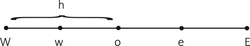
Next, we adopt a Jacobi iteration scheme to approximate the solution of (58(58) ${\int }_0^T{u}_x{w}_x\mathrm{d}t+\lambda Z^{\mathrm{\prime }}(k^{\mathrm{\prime }})=0.$(58) ). The advantage of the use of this algorithm is that it can look for the steady solution directly, and it is easy to implementation. Now, let us discretize the term $Z^{\mathrm{\prime }}(k^{\mathrm{\prime }})$. As shown in Figure 1, at a given point o, let E and W denote the two adjoint points, and let e and w be the corresponding two midway points.

Figure 1. A target node o and its neighbours, the spatial step size is h.

Define $|\cdot {|}_{\beta }=\sqrt{|\cdot {|}^2+\beta }$, then $Z(k^{\mathrm{\prime }})$ can be written as $Z(k^{\mathrm{\prime }})=k^{\mathrm{\prime }}/|k^{\mathrm{\prime }}{|}_{\beta }$. By applying the central difference scheme to Z, we have (59) $Z^{\mathrm{\prime }}\approx (Z_e-Z_w)/h,$(59) where h is the spatial step size. Next, we generate further approximations for Z at the two midway points $Z_e\approx k_e^{\mathrm{\prime }}/|k_e^{\mathrm{\prime }}{|}_{\beta }\text{ and }{Z}_w\approx k_w^{\mathrm{\prime }}/|k_w^{\mathrm{\prime }}{|}_{\beta },$ here $k_e^{\mathrm{\prime }}$ and $k_w^{\mathrm{\prime }}$ are approximated by $k_e^{\mathrm{\prime }}\approx (k_E-k_o)/h\mathrm{and}{k}_w^{\mathrm{\prime }}\approx (k_o-k_W)/h.$

Then, at a target point o, $Z^{\mathrm{\prime }}(k^{\mathrm{\prime }})$ can be discretized by (60) $Z^{\mathrm{\prime }}(k^{\mathrm{\prime }})\approx -\frac{1}{|k_e^{\mathrm{\prime }}{|}_{\beta }}\frac{k_o-k_E}{h^2}-\frac{1}{|k_w^{\mathrm{\prime }}{|}_{\beta }}\frac{k_o-k_W}{h^2}.$(60) Furthermore, by substituting (60(60) $Z^{\mathrm{\prime }}(k^{\mathrm{\prime }})\approx -\frac{1}{|k_e^{\mathrm{\prime }}{|}_{\beta }}\frac{k_o-k_E}{h^2}-\frac{1}{|k_w^{\mathrm{\prime }}{|}_{\beta }}\frac{k_o-k_W}{h^2}.$(60) ) into (58(58) ${\int }_0^T{u}_x{w}_x\mathrm{d}t+\lambda Z^{\mathrm{\prime }}(k^{\mathrm{\prime }})=0.$(58) ), we obtain (61) $-\lambda [\frac{1}{|k_e^{\mathrm{\prime }}{|}_{\beta }}\frac{k_o-k_E}{h^2}+\frac{1}{|k_w^{\mathrm{\prime }}{|}_{\beta }}\frac{k_o-k_W}{h^2}]+{\int }_0^T{u}_x{w}_x\mathrm{d}t=0.$(61) Let $A_e=\frac{1}{|k_e^{\mathrm{\prime }}{|}_{\beta }},A_w=\frac{1}{|k_w^{\mathrm{\prime }}{|}_{\beta }},$ then (61(61) $-\lambda [\frac{1}{|k_e^{\mathrm{\prime }}{|}_{\beta }}\frac{k_o-k_E}{h^2}+\frac{1}{|k_w^{\mathrm{\prime }}{|}_{\beta }}\frac{k_o-k_W}{h^2}]+{\int }_0^T{u}_x{w}_x\mathrm{d}t=0.$(61) ) is equivalent to (62) $k_o=\frac{A_e}{A_e+A_w}{k}_E+\frac{A_w}{A_e+A_w}{k}_W+\frac{h^2}{\lambda }\frac{{\int }_0^T{u}_x{w}_x\mathrm{d}t}{A_e+A_w}.$(62) Let $B=A_e+A_w$ and substituting it into (62(62) $k_o=\frac{A_e}{A_e+A_w}{k}_E+\frac{A_w}{A_e+A_w}{k}_W+\frac{h^2}{\lambda }\frac{{\int }_0^T{u}_x{w}_x\mathrm{d}t}{A_e+A_w}.$(62) ), we have (63) $k_o=\frac{A_e}{B}{k}_E+\frac{A_w}{B}{k}_W+\frac{h^2}{\lambda B}{\int }_0^T{u}_x{w}_x\mathrm{d}t.$(63) Then the Gauss–Jacobi iteration scheme[23] can be applied for (63(63) $k_o=\frac{A_e}{B}{k}_E+\frac{A_w}{B}{k}_W+\frac{h^2}{\lambda B}{\int }_0^T{u}_x{w}_x\mathrm{d}t.$(63) ). At each step n, we update $k^{(n)}$ to $k^{(n+1)}$ by (64) $k_o^{(n+1)}=\frac{A_e^{(n)}}{B^{(n)}}{k}_E^{(n)}+\frac{A_w^{(n)}}{B^{(n)}}{k}_W^{(n)}+\frac{h^2}{\lambda B^{(n)}}{\int }_0^T{u}_x^{(n)}{w}_x^{(n)}\mathrm{d}t,$(64) where $k^{(n)}=k(x^{(n)})$. The integral term in the right-hand side ${\int }_0^T{u}_x{v}_x\mathrm{d}t$ can be computed by Simpson's rule or trapezoidal rule.

From the analysis above, we propose the following algorithm:

1. Choose a function $k(x)=k^{(0)}(x)$ as an initial value of iteration.

2. Solve Equation (1(1) $\begin{array}{ll}{u}_t-(k(x)u_x{)}_x=f(x,t),& (x,t)\in D_T,\\ u(x,0)=\phi (x),& x\in [0,l],\\ u(0,t)=u(l,t)=0,& t\in [0,T],\end{array}$(1) ) to obtain $u^{(n)}(x,t)$, where $k(x)=k^{(n)}(x)$.

3. Solve Equation (29(29) $\begin{array}{ll}-w_t-(k(x)w_x{)}_x=0,& (x,t)\in D_T,\\ w(x,T)=u(x,T)-s(x),& x\in [0,l],\\ w(0,t)=w(l,t)=0,& t\in [0,T].\end{array}$(29) ) to obtain $w^{(n)}(x,t)$, where $w^{(n)}(x,T)=u^{(n)}(x,T)-s(x),$ and compute ${\int }_0^T{u}_x^{(n)}{v}_x^{(n)}\mathrm{d}t$.

4. Compute $k_o^{(n+1)}=\frac{A_e^{(n)}}{B^{(n)}}{k}_E^{(n)}+\frac{A_w^{(n)}}{B^{(n)}}{k}_W^{(n)}+\frac{h^2}{\lambda B^{(n)}}{\int }_0^T{u}_x^{(n)}{w}_x^{(n)}\mathrm{d}t,$ to obtain the next value of iteration, where the boundary points of k are handled by the Neumann boundary condition.

5. Select an arbitrarily small positive constant α, compute $\Vert k^{(n+1)}(x)-k^{(n)}(x){\Vert }_{\mathrm{\infty }}$ and compare it with α. If $\Vert k^{(n+1)}(x)-k^{(n)}(x){\Vert }_{\mathrm{\infty }}<\alpha ,$ stop and take $\overline{k}(x)=k^{(n)}(x)$. Otherwise, let n = n + 1, go to step 2 and go on computing by the induction principle.

5. Numerical experiments

In this section we carried out some numerical experiments to examine the theory and algorithm presented in the above sections.

The forward problem (1(1) $\begin{array}{ll}{u}_t-(k(x)u_x{)}_x=f(x,t),& (x,t)\in D_T,\\ u(x,0)=\phi (x),& x\in [0,l],\\ u(0,t)=u(l,t)=0,& t\in [0,T],\end{array}$(1) ) and (29(29) $\begin{array}{ll}-w_t-(k(x)w_x{)}_x=0,& (x,t)\in D_T,\\ w(x,T)=u(x,T)-s(x),& x\in [0,l],\\ w(0,t)=w(l,t)=0,& t\in [0,T].\end{array}$(29) ) are solved by the finite volume method. In all the numerical experiments, we take $T=1,\beta =0.0001,\tau =T/100,h=l/100,\delta =0.01,$ where τ is the time step size, h is the spatial step size and δ is the noise level. The regularization parameters used in this paper are chosen by the Morozov discrepancy principle (see, e.g. [1,40]). The synthetic data is generated in the following form $s^{\delta }(x)=u^{\delta }(x,T)=u(x,T)[1+\delta \times \text{random }(x)].$ where random$(x)$ denotes the uniform distribution in $[-1,1]$. The source term $f(x,t)$ and the initial term $\phi (x)$ in Equation (1(1) $\begin{array}{ll}{u}_t-(k(x)u_x{)}_x=f(x,t),& (x,t)\in D_T,\\ u(x,0)=\phi (x),& x\in [0,l],\\ u(0,t)=u(l,t)=0,& t\in [0,T],\end{array}$(1) ) are taken as $f(x,t)=(\sin x-2\sin x{\cos }^{2}x+{\sin }^{3}x)e^t,$ and $\phi (x)=\sin x,$ respectively.

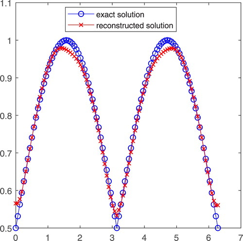
Example 5.1

In the first example, we take $k(x)=\frac{1}{2}|\sin x|+\frac{1}{2},x\in [0,2\pi ].$ The initial value of iteration $k^{(0)}=1$ and the regularization parameter $\lambda =0.005$.

Figure 2 shows the reconstructions of $k(x)$, where the '–o–' line is the exact coefficient and the '–x–' line is the inversion coefficient. It can be seen that the diffusion coefficient $k(x)$ is non-smooth at $x=\pi$, and the inversion algorithm can give a satisfactory result.

Figure 2. Reconstructions of the coefficient $k(x)$ in example 1, $k^{(0)}(x)=1$, $\lambda =0.005$.

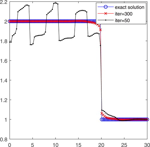
Example 5.2

In the second example, we take $k(x)=\{\begin{array}{ll}2,& 0⩽x<20,\\ 1,& 20⩽x⩽30.\end{array}$ The initial value of iteration $k^{(0)}=1$ and the regularization parameter $\lambda =0.05$.

In this case, the change of $k(x)$ is mainly reflected on the discontinuous point. In order to show the inversion process of the total variation algorithm, we compare the numerical results of different iteration times. As shown in Figure 3, the '–o–' line is the exact coefficient, and the '–•–' line and the '–x–' line are the inversion coefficient after 50 iterations and 300 iterations, respectively. From the numerical result, we can see that our algorithm works well for the discontinuous case.

Figure 3. Reconstructions of the coefficient $k(x)$ in example 2, $k^{(0)}(x)=1$, $\lambda =0.05$.

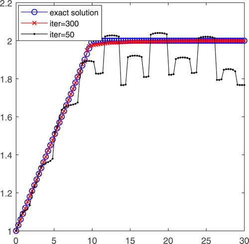
Example 5.3

In the third example, we take $k(x)=\{\begin{array}{ll}{\displaystyle \frac{1}{10}}x+1,& 0⩽x<10,\\ 2,& 10⩽x⩽30.\end{array}$ The initial value of iteration $k^{(0)}=1$ and the regularization parameter $\lambda =0.01$.

Figure 4 shows different iteration times of the numerical results. The '–o–' line is the exact coefficient $k(x)$. The '–•–' line is the inversion coefficient $\overline{k}(x)$ after 50 iteration times. The '–x–' line is the inversion coefficient $\overline{k}(x)$ after 300 iteration times. It can be seen that after 300 iterations the coefficient $k(x)$ is recovered very well.

Figure 4. Reconstructions of the coefficient $k(x)$ in example 3, $k^{(0)}(x)=1$, $\lambda =0.01$.

6. Conclusions

In this paper, we investigated an inverse problem of identifying an unknown coefficient of a parabolic equation. The total variation regularization method is proposed to deal with the ill-posedness. By transforming the problem into an optimal control problem, the existence, necessary condition as well as the stability of the minimizer of the control functional are established. Through a modification of the necessary condition into an equality form, we designed a Jacobi iteration scheme to obtain numerical solution. The numerical experiments show that this algorithm is effective and stable to reconstruct non-smooth solutions.

Disclosure statement

No potential conflict of interest was reported by the author(s).

Additional information

Funding

This work was supported by the NNSF of China (National Natural Science Foundation of China) [grant number 11771068].

References

- Kirsch A. An introduction to the mathematical theory of inverse problems. New York: Springer; 2011.
- Deng Z, Yang L, Yu J, et al. An inverse problem of identifying the coefficient in a nonlinear parabolic equation. Nonlinear Anal Theory Methods Appl. 2009;71(12):6212–6221. doi: 10.1016/j.na.2009.06.014
- Sun J. An eigenvalue method using multiple frequency data for inverse scattering problems. Inverse Problems. 2012;28(2):025012. doi: 10.1088/0266-5611/28/2/025012
- Demir A, Hasanov A. Identification of the unknown diffusion coefficient in a linear parabolic equation by the semigroup approach. J Math Anal Appl. 2008;340(1):5–15. doi: 10.1016/j.jmaa.2007.08.004
- Isakov V, Kindermann S. Identification of the diffusion coefficient in a one-dimensional parabolic equation. Inverse Problems. 2000;16(3):665–680. doi: 10.1088/0266-5611/16/3/309
- Keung YL, Zou J. Numerical identifications of parameters in parabolic systems. Inverse Problems. 1998;14(1):83–100. doi: 10.1088/0266-5611/14/1/009
- Deng Z, Yang L, Yu J, et al. Identifying the diffusion coefficient by optimization from the final observation. Appl Math Comput. 2013;219(9):4410–4422.
- Chen Q, Liu JJ. Solving an inverse parabolic problem by optimization from final measurement data. J Comput Appl Math. 2006;193(1):183–203. doi: 10.1016/j.cam.2005.06.003
- Cheng J, Liu JJ. A quasi Tikhonov regularization for a two-dimensional backward heat problem by a fundamental solution. Inverse Problems. 2008;24(6):065012. doi: 10.1088/0266-5611/24/6/065012
- Deng Z, Yang L. An inverse problem of identifying the radiative coefficient in a degenerate parabolic equation. Chin Ann Math Ser B. 2014;35(1):355–382. doi: 10.1007/s11401-014-0836-x
- Egger H, Engl HW. Tikhonov regularization applied to the inverse problem of option pricing: convergence analysis and rates. Inverse Problems. 2005;21(3):1027–1045. doi: 10.1088/0266-5611/21/3/014
- Yang L, Dehghan M, Yu J, et al. Inverse problem of time-dependent heat sources numerical reconstruction. Math Comput Simul. 2011;81(8):1656–1672. doi: 10.1016/j.matcom.2011.01.001
- Yang L, Yu JN, Deng Z. An inverse problem of identifying the coefficient of parabolic equation. Appl Math Model. 2008;32(10):1984–1995. doi: 10.1016/j.apm.2007.06.025
- Deng Z, Yang L, Yao B, et al. An inverse problem of determining the shape of rotating body by temperature measurements. Appl Math Model. 2018;59:464–482. doi: 10.1016/j.apm.2018.02.002
- Yang L, Deng Z, Hon Y. Simultaneous identification of unknown initial temperature and heat source. Dyn Syst Appl. 2016;25(1–4):583–602.
- Yamamoto M, Zou J. Simultaneous reconstruction of the initial temperature and heat radiative coefficient. Inverse Problems. 2001;17(4):1181–1202. doi: 10.1088/0266-5611/17/4/340
- Isakov V. Inverse parabolic problems with the final overdetermination. Commun Pure Appl Math. 1991;44(2):185–209. doi: 10.1002/cpa.3160440203
- Jiang D, Feng H, Zou J. Convergence rates of Tikhonov regularizations for parameter identification in a parabolic-elliptic system. Inverse Problems. 2012;28(10):104002. doi: 10.1088/0266-5611/28/10/104002
- Deng Z, Hon Y, Yang L. An optimal control method for nonlinear inverse diffusion coefficient problem. J Optim Theory Appl. 2014;160(3):890–910. doi: 10.1007/s10957-013-0302-z
- Deng Z, Yu J, Yang L. Identifying the coefficient of first-order in parabolic equation from final measurement data. Math Comput Simulat. 2008;77(4):421–435. doi: 10.1016/j.matcom.2008.01.002
- Isakov V. Inverse problems for partial differential equations. New York: Springer; 2006.
- Tikhonov A, Goncharsky AV, Stepanov VV, et al. Numerical methods for the solution of ill-posed problems. Dordrecht: Springer; 1995.
- Shen J, Chan T. Mathematical models for local nontexture inpaintings. SIAM J Appl Math. 2002;62(3):1019–1043. doi: 10.1137/S0036139900368844
- Rudin LI, Osher S, Fatemi E. Nonlinear total variation based noise removal algorithms. Phys D. 1992;60(1):259–268. doi: 10.1016/0167-2789(92)90242-F
- Hào DN, Quyen TN. Convergence rates for total variation regularization of coefficient identification problems in elliptic equations I. Inverse Problems. 2011;27(7):075008. doi: 10.1088/0266-5611/27/7/075008
- Wunderli T. A partial regularity result for an anisotropic smoothing functional for image restoration in BV-space. J Math Anal Appl. 2008;339(2):1169–1178. doi: 10.1016/j.jmaa.2007.07.013
- Giusti E. Minimal surfaces and functions of bounded variation. Boston: Birkhäuser; 1984.
- Bachmayr M, Burger M. Iterative total variation schemes for nonlinear inverse problems. Inverse Problems. 2009;25(10):105004. doi: 10.1088/0266-5611/25/10/105004
- Chan TF, Tai X. Identification of discontinuous coefficients in elliptic problems using total variation regularization. SIAM J Sci Comput. 2003;25(3):881–904. doi: 10.1137/S1064827599326020
- Dou Y, Han B. Total variation regularization for the reconstruction of a mountain topography. Appl Numer Math. 2012;62(1):1–20. doi: 10.1016/j.apnum.2011.09.004
- Hào DN, Quyen TN. Convergence rates for total variation regularization of coefficient identification problems in elliptic equations II. J Math Anal Appl. 2012;388(1):593–616. doi: 10.1016/j.jmaa.2011.11.008
- Li L, Han B. A new iteratively total variational regularization for nonlinear inverse problems. J Comput Appl Math. 2016;298:40–52. doi: 10.1016/j.cam.2015.11.033
- Pan B, Xu D, Xu Y, et al. TV-like regularization for backward parabolic problems. Math Methods Appl Sci. 2017;40(4):957–969. doi: 10.1002/mma.4027
- Wang L, Liu JJ. Total variation regularization for a backward time-fractional diffusion problem. Inverse Problems. 2013;29(11):115013. doi: 10.1088/0266-5611/29/11/115013
- Osher S, Burger M, Goldfarb D, et al. An iterative regularization method for total variation-based image restoration. Multiscale Model Simul. 2005;4(2):460–489. doi: 10.1137/040605412
- Acar R, Vogel CR. Analysis of bounded variation penalty methods for ill-posed problems. Inverse Problems. 1994;10(6):1217–1229. doi: 10.1088/0266-5611/10/6/003
- Evans L. Partial differential equations. 2nd ed. Graduate Studies in Mathematics; Providence: American Mathematical Society; 2010.
- Friedman A. Partial differential equations of parabolic type. Englewood Cliffs, NJ: Prentice-Hall; 1964.
- Ladyzhenskaia OA, Solonnikov VA, Ural'ceva NN. Linear and quasi-linear equations of parabolic type. Providence (RI): American Mathematical Society; 1968.
- Xiao T, Yu S, Wang Y. Numerical solution for inverse problems. Beijing: Science Press; 2003.