Non-iterative two-step method for solving scalar inverse 3D diffraction problem

Abstract

The scalar problem of reconstruction of an unknown refractive index of an inhomogeneous solid is considered. The original boundary value problem for the Helmholtz equation with an unknown refractive index is reduced to the source-type integral equation. The solution to the inverse problem is obtained in two steps. First, the integral equation of the first kind is solved in the inhomogeneity domain using measurements of the total field outside the domain. The uniqueness of a solution to the integral equation of the first kind is proved in a special class of functions. Second, the sought-for refractive index is explicitly expressed via the found solution and the total field. The two-step method was verified by solving a test problem with a given refractive index. Procedures for refining approximate solutions were proposed and implemented. Efficiency of the proposed method was approved by comparison between the exact solution and the approximate ones.

Keywords:

• Refractive index reconstruction
• integral equations
• solution uniqueness

2010 Mathematics Subject Classifications:

• 45Q05
• 65N21
• 31B10

1. Introduction

The paper deals with a non-iterative two-step method (TSM) for solving the scalar inverse problem of diffraction by an inhomogeneous solid located in the unbounded homogeneous space ${\mathbb{R}}^3.$

The importance of the considered problem is due to a wide range of applications such as microwave tomography or reconstruction of characteristics of composite materials.

Among theoretical works dedicated to theoretical investigation of existence and uniqueness of solutions to inverse problems, we only mention [1] which contains an extensive and up-to-date bibliography on the subject.

Common numerical methods for studying inverse problems are based on solving hyperbolic systems of differential equations in the time domain using finite difference or finite element methods, with subsequent minimization of the corresponding functionals and Tikhonov regularization [2–10].

There have recently appeared several works in which novel iterative globally convergent algorithms were proposed. The approaches presented in [11, 12] are based on the construction of weighted globally strictly convex cost functionals. Eliminating the phenomenon of multiple local minima of cost functionals provides the global convergence to the correct solution of the gradient projection method.

The volume singular integral equation method is an alternative approach to solving the inverse problems of electrodynamics and acoustics (see e.g. [7, 13–20]).

In this paper, we use the integral equation which is well-known as the ‘source-type integral equation’ (STIE). Common techniques for numerical solving STIE involve minimization of special error functionals (see, e.g. [13, 20]) and require a good initial approximation to avoid local minima of the cost functionals. The idea of TSM is in direct numerical solving the linear source-type integral equation with subsequent explicit evaluation of the sought-for contrast function.

The article consists of four sections.

In Section 2, we rigorously formulate the forward problem of diffraction and give main theoretical results of its investigation. Note that some results are similar to the ones described in [15]. The major difference from [15] is that we consider the quasiclassical setting of the boundary value problem (BVP) for the Helmholtz equation, assuming that a solution should satisfy additional smoothness conditions. Then, we write the integral Lippmann–Schwinger equation (LSIE) with respect to the unknown total field $u=u_0+u_s$ in the inhomogeneity region Q. The operator of the equation is well studied [15] and is known to be a Fredholm operator of index zero. Further, we show that any solution $u\in L_2\left(Q\right)$ to LSIE with a smooth right-hand side represents in fact a quasiclassical solution to the original BVP. Thus, we obtain that the BVP for the Helmholtz equation is equivalent to the system of integral equations used for recovering the refractive index in Section 3 of the article.

Section 3 describes theoretical investigation of the inverse scattering problem. We assume that the incident wave is the field of a point source located outside $\overline{Q}$, whereas the sought-for refractive index $k\left(x\right)$ is assumed to be a continuous or piecewise Hölder function in Q such that $|k\left(x\right)|\ge \tilde{k}>k_0$. Here $k_0>0$ is the given wave number of the free space ${\mathbb{R}}^3.$ To find the function $k\left(x\right),$ we consider STIE under assumption that the near field data is determined in some bounded domain D such that $\overline{Q}\cap \overline{D}=\mathrm{\varnothing }$, whereas the source point $x_0$ is outside $\overline{D}\cup \overline{Q}$.

In Section 3.2, we describe TSM. The first step is in direct solving the STIE. Note that we introduce the current $J\left(x\right)=\left(k^2\right(x)-k_0^2)u\left(x\right)$ in the inhomogeneity domain Q and then solve STIE with respect to J using the near field data given in D. The second step of TSM involves direct calculation of the sought-for solution $k\left(x\right)$ via the given functions $J\left(x\right)$, $u\left(x\right)$ and $u_0\left(x\right)$ using the LSIE in the domain Q.

Solving STIE, one faces the well-known problem of non-uniqueness of a solution to STIE. In Section 3.2, we give an example of a smooth non-trivial solution to the homogeneous STIE. However, unique solvability is then proved in special function classes. In [21], we introduced the class of piecewise-constant functions with rectangular support. In the present work, we describe much wider classes of solutions which can be represented by linear combinations of compactly supported basis functions.

The main theoretical result presented in Section 3.3 is the theorem on uniqueness of a solution to the STIE that was first announced in [22]. As in [21, 23], we prove that, for almost all values of the wave number $k_0>0,$ the STIE has at most one solution in the introduced classes of functions.

In Section 4, we describe conditions of numerical tests, show in several figures the obtained approximate solutions, and explain the algorithm of solutions' refinement. It is clear that in a realistic experiment, one cannot use some ‘pure’ field data which can be analytically modelled. That is why we simulate noisy near filed data which results in disturbing a solution, as well as appearing of false inhomogeneities and loss of the true ones. We propose several techniques for obtaining accurate solutions: extraneous noise screening out (filtering the input near filed data), analysis of disturbed solutions obtained for various wave frequencies with the further construction of an accurate approximate solution, and final postprocessing (levelling of the sought-for function).

The last section of the paper contains proofs of the theorems.

2. Forward scattering problem: statement and main results

We consider a bounded solid Q located in the isotropic homogeneous space ${\mathbb{R}}^3$. The lossless homogeneous medium ${\mathbb{R}}^3\setminus \overline{Q}$ is characterized by a given wave number $k_0>0.$

The inhomogeneity domain Q is filled with isotropic inhomogeneous medium. We assume that Q can be represented by a union of several subdomains $Q_l$ ($l=1,\dots ,N$), $\overline{Q}={\cup }_l{\overline{Q}}_l,Q_l\cap Q_{l^{\prime }}=\mathrm{\varnothing }\mathrm{f}\mathrm{o}\mathrm{r}l\ne l^{\prime },$ and $\mathrm{\partial }{Q}_l$ is a piecewise smooth boundary that consists of a finite number of surfaces of the class $C^{\mathrm{\infty }}$.

We consider inhomogeneities of the domain Q of two types. Inhomogeneities of the first type are presented by continuous functions $k\left(x\right)=n\left(x\right)k_0\in C\left(\overline{Q}\right),$ whereas inhomogeneities of the second type are described by piecewise-continuous functions $k\left(x\right).$ In the latter case, we set (1) $k\left(x\right)=k_l\left(x\right),x\in Q_l,$(1) where $k_l\in C^{\alpha }\left(Q_l\right)$ are arbitrary Hölder continuous functions. At the points of the boundaries $\mathrm{\partial }{Q}_l$, the function $k\left(x\right)$ can be defined via the one-sided limit from any side of the surface.

Introducing the set of characteristic functions (2) ${\chi }_l\left(x\right)=\left\{\begin{array}{ll}1,& x\in Q_l,\\ 0,& x\notin Q_l,\end{array}\right.$(2) we can define the function $k\left(x\right)$ at any point $x\in Q$ by the equality (3) $k\left(x\right)=\sum _l{k}_l\left(x\right){\chi }_l\left(x\right).$(3)

We define $E_Q$ as the union of all edges of the solids $Q_l$ and introduce the following notation: (4) $Q_l^{\prime }:=Q_l\setminus E_Q,Q^{\prime }:=Q\setminus E_Q.$(4)

We use the representation of the total field $U(x,t)$ via the sum $U(x,t)=U_0(x,t)+U_s(x,t)$ of the incident wave $U_0$ and the scattered field $U_s.$ All fields depend on time harmonically: $U_0(x,t)=u_0\left(x\right){\mathrm{e}}^{-\mathrm{i}\omega t}$ and $U_s(x,t)=u_s\left(x\right){\mathrm{e}}^{-\mathrm{i}\omega t}$.

The function (5) $u_0\left(x\right)=\frac{{\mathrm{e}}^{\mathrm{i}{k}_0|x-x_0|}}{4\pi |x-x_0|},x_0\notin \overline{Q},$(5) describes the incident field of a point source that satisfies the Helmholtz equation $(\mathrm{△}+k_0^2)u_0\left(x\right)=-\delta (x-x_0)$ and the Sommerfeld radiation condition.

Definition 2.1

The forward scattering problem in the rigorous mathematical statement is to find a solution $u\left(x\right)$ to the following boundary value problem: (6) $\left({\mathcal{P}}_1\right)\left\{\begin{array}{l}(\mathrm{△}+k_l^2(x\left)\right)u\left(x\right)=0,x\in Q_l,\\ (\mathrm{△}+k_0^2)u\left(x\right)=-\delta (x-x_0),x\in {\mathbb{R}}^3\setminus \overline{Q},\\ {\left.\left[u\right]\right|}_{\mathrm{\partial }{Q}_l}=0,{\left.\left[\frac{\mathrm{\partial }u}{\mathrm{\partial }\mathbf{n}}\right]\right|}_{\mathrm{\partial }{Q}_l^{\prime }}=0,\\ u\in H_{loc}^1({\mathbb{R}}^3\setminus \{x_0\left\}\right),\\ \frac{\mathrm{\partial }{u}_s}{\mathrm{\partial }r}=i{k}_0{u}_s+o\left(\frac{1}{r}\right),r=|x|\to +\mathrm{\infty }.\end{array}\right.$(6) Here ${\left.\left[u\right]\right|}_{\mathrm{\partial }{Q}_l}$ denotes the jump of the function u, i.e. the difference of traces of u on $\mathrm{\partial }{Q}_l$ from the inside and the outside of the domain $Q_l$.

Definition 2.2

Any solution to the problem $\left({\mathcal{P}}_1\right)$ that satisfies the conditions (7) $u\in C^1({\mathbb{R}}^3\setminus \{x_0\left\}\right)\bigcap _l{C}^2\left(Q_l\right)\bigcap C^{\mathrm{\infty }}({\mathbb{R}}^3\setminus (\overline{Q}\cup \left\{x_0\right\}\left)\right),$(7) is a quasiclassical solution to the forward scattering problem.

Remark 2.1

Note that a solution to problem $\left({\mathcal{P}}_1\right)$ should be understood in the distributional sense due to the choice of the incident field and the equation considered in ${\mathbb{R}}^3\setminus \overline{Q}.$ Nevertheless, we formulate the Helmholtz equation in $Q_l$ and the Sommerfeld radiation condition in the classical sense assuming that any solution to $\left({\mathcal{P}}_1\right)$ is in fact a smooth function at any point $x\ne x_0.$

The problem $\left({\mathcal{P}}_1\right)$ can be reduced [15] to the following system of integral equations: (8) $\begin{array}{rl}& u\left(x\right)-{\int }_Q\left(k^2\right(y)-k_0^2)G(x,y)u\left(y\right)\mathrm{d}y=u_0\left(x\right),x\in Q,\end{array}$(8) (9) $\begin{array}{rl}& u\left(x\right)=u_0\left(x\right)+{\int }_Q\left(k^2\right(y)-k_0^2)G(x,y)u\left(y\right)dy,x\in {\mathbb{R}}^3\setminus (Q\cup \{x_0\left\}\right).\end{array}$(9)

Definition 2.3

The integral statement of the forward diffraction problem is understood as the system $\left({\mathcal{P}}_2\right)$ consisting of equation (8(8) $\begin{array}{rl}& u\left(x\right)-{\int }_Q\left(k^2\right(y)-k_0^2)G(x,y)u\left(y\right)\mathrm{d}y=u_0\left(x\right),x\in Q,\end{array}$(8) ) in the domain Q and representation (9(9) $\begin{array}{rl}& u\left(x\right)=u_0\left(x\right)+{\int }_Q\left(k^2\right(y)-k_0^2)G(x,y)u\left(y\right)dy,x\in {\mathbb{R}}^3\setminus (Q\cup \{x_0\left\}\right).\end{array}$(9) ) in ${\mathbb{R}}^3\setminus (Q\cup \{x_0\left\}\right)$.

The operator in (8(8) $\begin{array}{rl}& u\left(x\right)-{\int }_Q\left(k^2\right(y)-k_0^2)G(x,y)u\left(y\right)\mathrm{d}y=u_0\left(x\right),x\in Q,\end{array}$(8) ) denoted by $\mathcal{I}-\mathcal{A}$ is treated as a mapping in the $L_2\left(Q\right)$ space.

First, it can be shown that any solution $u\left(x\right)$ of the problem $\left({\mathcal{P}}_2\right)$ satisfies the smoothness conditions formulated in the quasiclassical statement of the problem.

Theorem 2.4

Let (8(8) $\begin{array}{rl}& u\left(x\right)-{\int }_Q\left(k^2\right(y)-k_0^2)G(x,y)u\left(y\right)\mathrm{d}y=u_0\left(x\right),x\in Q,\end{array}$(8) ) have a solution $u\in L_2\left(Q\right).$ Then, the total field $u\left(x\right)$ extended outside Q by (9(9) $\begin{array}{rl}& u\left(x\right)=u_0\left(x\right)+{\int }_Q\left(k^2\right(y)-k_0^2)G(x,y)u\left(y\right)dy,x\in {\mathbb{R}}^3\setminus (Q\cup \{x_0\left\}\right).\end{array}$(9) ) satisfies smoothness conditions (7(7) $u\in C^1({\mathbb{R}}^3\setminus \{x_0\left\}\right)\bigcap _l{C}^2\left(Q_l\right)\bigcap C^{\mathrm{\infty }}({\mathbb{R}}^3\setminus (\overline{Q}\cup \left\{x_0\right\}\left)\right),$(7) ).

The next two theorems are on the equivalency between two formulations of the forward scattering problem, and on uniqueness of the quasiclassical solution to $\left({\mathcal{P}}_1\right)$.

Theorem 2.5

The problems $\left({\mathcal{P}}_1\right)$ and $\left({\mathcal{P}}_2\right)$ are equivalent. More precisely, if $u\left(x\right)$ is a quasiclassical solution to the problem $\left({\mathcal{P}}_1\right)$ then u satisfies (8(8) $\begin{array}{rl}& u\left(x\right)-{\int }_Q\left(k^2\right(y)-k_0^2)G(x,y)u\left(y\right)\mathrm{d}y=u_0\left(x\right),x\in Q,\end{array}$(8) ) and (9(9) $\begin{array}{rl}& u\left(x\right)=u_0\left(x\right)+{\int }_Q\left(k^2\right(y)-k_0^2)G(x,y)u\left(y\right)dy,x\in {\mathbb{R}}^3\setminus (Q\cup \{x_0\left\}\right).\end{array}$(9) ). Vise versa, if $u\in L_2\left(Q\right)$ is a solution to the IE (8(8) $\begin{array}{rl}& u\left(x\right)-{\int }_Q\left(k^2\right(y)-k_0^2)G(x,y)u\left(y\right)\mathrm{d}y=u_0\left(x\right),x\in Q,\end{array}$(8) ), then the total field $u\left(x\right)$ extended to ${\mathbb{R}}^3\setminus \left\{x_0\right\}$ by (9(9) $\begin{array}{rl}& u\left(x\right)=u_0\left(x\right)+{\int }_Q\left(k^2\right(y)-k_0^2)G(x,y)u\left(y\right)dy,x\in {\mathbb{R}}^3\setminus (Q\cup \{x_0\left\}\right).\end{array}$(9) ) is a quasiclassical solution to the problem $\left({\mathcal{P}}_1\right)$.

Theorem 2.6

For any $\mathrm{\Im }k\left(x\right)\ge 0$ the problem $\left({\mathcal{P}}_1\right)$ has at most one quasiclassical solution.

The proof of Theorem 2.6 can be found in [24, 25].

From Theorems 2.5 and 2.6, it follows that $\mathcal{I}-\mathcal{A}$ is an invertible operator. For any $u\in L_2\left(Q\right)$ we have $\mathcal{A}u\in H^2\left(Q\right)$ which implies that $\mathcal{A}$ is a compact operator in $L_2\left(Q\right).$ Let $u_0\equiv 0$ in ${\mathbb{R}}^3.$ Then the boundary value problem $\left({\mathcal{P}}_1\right)$ has only the trivial solution (see Theorem 2.6). By virtue of the equivalency between $\left({\mathcal{P}}_1\right)$ and $\left({\mathcal{P}}_2\right),$ u = 0 is the only solution to the IE $(\mathcal{I}-\mathcal{A})u=0$. Hence, $(\mathcal{I}-\mathcal{A}):L_2\left(Q\right)\to L_2\left(Q\right)$ is an injective Fredholm operator with index zero. Thus, we arrive at

Theorem 2.7

The operator $(\mathcal{I}-\mathcal{A}):L_2\left(Q\right)\to L_2\left(Q\right)$ is continuously invertible.

Thus, summarizing Theorems 2.4–2.7, we derive that the forward diffraction problem has a unique quasiclassical solution.

3. Refractive index reconstruction

3.1. Statement of the inverse problem

Consider an inhomogeneous solid (10) $Q=\{x=(x_1,x_2,x_3):a_1<x_1<b_1,a_2<x_2<b_2,a_3<x_3<b_3\}$(10) and assume that Q is characterized by an unknown refractive index $n\left(x\right)=k\left(x\right)/k_0$ which can be a continuous function in $\overline{Q},$ or a piecewise-continuous function. In the latter case, $k\left(x\right)$ is assumed to be a piecewise Hölder function in Q such that $k\left(x\right)\in C^{\alpha }\left({\overline{Q}}_l\right),$ where $Q_l\subset Q$.

Introduce a bounded domain D, $\overline{D}\cap \overline{Q}=\mathrm{\varnothing }$. The values of the total field (11) $U(x,t)=U_0(x,t)+U_s(x,t),U_s(x,t)=u_s{\mathrm{e}}^{-\mathrm{i}\omega t},$(11) are given at the points $x\in D$ at a frequency ω.

The incident wave is (12) $U_0(x,t)=\frac{{\mathrm{e}}^{\mathrm{i}{k}_0|x-x_0|}}{4\pi |x-x_0|}{\mathrm{e}}^{-\mathrm{i}\omega t},$(12) where $x_0$ is an arbitrary source point such that $x_0\notin \overline{Q}\cup \overline{D}.$

In the proposed statement of the inverse diffraction problem, we use the system $\left({\mathcal{P}}_2\right)$ of integral equalities which represent the relation between the total field $u\left(x\right)$ and the function $k\left(x\right).$ It is shown above that problems $\left({\mathcal{P}}_1\right)$ and $\left({\mathcal{P}}_2\right)$ are equivalent.

Definition 3.1

Statement of the inverse problem

Let $k\left(x\right),$ $x\in Q,$ be an unknown continuous (or piecewise Hölder) function. Assume that inequality (13) $|k\left(x\right)|\ge \tilde{k}>k_0$(13) holds in $\overline{Q}$. The inverse problem of diffraction in the integral formulation is to find the function $k\left(x\right)$ in the entire domain Q from equation (14) ${\int }_Q\left(k^2\right(y)-k_0^2)G(x,y)u\left(y\right)\mathrm{d}y=u\left(x\right)-u_0\left(x\right),x\in D,$(14) using given values of the total field $u\left(x\right),$ $x\in D,$ and taking into account the equation (8(8) $\begin{array}{rl}& u\left(x\right)-{\int }_Q\left(k^2\right(y)-k_0^2)G(x,y)u\left(y\right)\mathrm{d}y=u_0\left(x\right),x\in Q,\end{array}$(8) ). (15) $u\left(x\right)-\dots \mathrm{t}\mathrm{o}\mathrm{b}\mathrm{e}\mathrm{d}\mathrm{e}\mathrm{l}\mathrm{e}\mathrm{t}\mathrm{e}\mathrm{d}$(15)

Remark 3.1

Inequality (13(13) $|k\left(x\right)|\ge \tilde{k}>k_0$(13) ) should not be treated as a restriction on considered domains. It merely describes the scatterer's refractive index that differs from the index of the free space which is a standard condition in acoustics and electrodynamics.

3.2. Formulation of TSM for solving the inverse problem

We introduce the function $J\left(x\right)=\left(k^2\right(x)-k_0^2)u\left(x\right)$ in the region Q and rewrite Equations (14(14) ${\int }_Q\left(k^2\right(y)-k_0^2)G(x,y)u\left(y\right)\mathrm{d}y=u\left(x\right)-u_0\left(x\right),x\in D,$(14) ) and (15(15) $u\left(x\right)-\dots \mathrm{t}\mathrm{o}\mathrm{b}\mathrm{e}\mathrm{d}\mathrm{e}\mathrm{l}\mathrm{e}\mathrm{t}\mathrm{e}\mathrm{d}$(15) ) as follows (16) $\begin{array}{rl}& {\int }_{Q}G(x,y)J\left(y\right)\mathrm{d}y=u\left(x\right)-u_0\left(x\right)=u_s\left(x\right),x\in D,\end{array}$(16) (17) $\begin{array}{rl}& \frac{J\left(x\right)}{k^2\left(x\right)-k_0^2}-{\int }_{Q}G(x,y)J\left(y\right)\mathrm{d}y=u_0\left(x\right),x\in Q.\end{array}$(17)

The proposed non-iterative TSM for reconstructing the unknown function $k\left(x\right)$ consists of two steps:

• using the given values of the incident wave $u_0\left(x\right)$ and the total field $u\left(x\right)$ in D, we find the solution $J\left(x\right)$ to (16(16) $\begin{array}{rl}& {\int }_{Q}G(x,y)J\left(y\right)\mathrm{d}y=u\left(x\right)-u_0\left(x\right)=u_s\left(x\right),x\in D,\end{array}$(16) ) in the domain Q;

• we evaluate the function $k\left(x\right)$ at points $x\in Q$ using equation(17(17) $\begin{array}{rl}& \frac{J\left(x\right)}{k^2\left(x\right)-k_0^2}-{\int }_{Q}G(x,y)J\left(y\right)\mathrm{d}y=u_0\left(x\right),x\in Q.\end{array}$(17) ).

It can be shown that the IE (16(16) $\begin{array}{rl}& {\int }_{Q}G(x,y)J\left(y\right)\mathrm{d}y=u\left(x\right)-u_0\left(x\right)=u_s\left(x\right),x\in D,\end{array}$(16) ) has multiple solutions which follows from the proposition below.

Proposition 3.2

For any $k_0$, there exist non-trivial solutions to the homogeneous integral equation ${\int }_{Q}G(x,y)J\left(y\right)\mathrm{d}y=0$.

Proof.

Consider an arbitrary domain Q and a smooth function that satisfies the homogeneous boundary conditions $\psi {|}_{\mathrm{\partial }Q}=\mathrm{\partial }\psi /\mathrm{\partial }\mathbf{n}{|}_{\mathrm{\partial }{Q}^{\prime }}=0$ (closed-form expressions of ψ can easily be given in cases of elementary shapes, i.e. parallelepipeds, balls, etc. [21]). Define $J\left(x\right)=-(\mathrm{△}+k_0^2)\psi$. By virtue of the boundary conditions for ψ one gets the representation $\psi \left(x\right)={\int }_{Q}G(x,y)J\left(y\right)\mathrm{d}y,x\in \overline{Q}.$ Introduce the potential $v\left(x\right)={\int }_{Q}G(x,y)J\left(y\right)\mathrm{d}y,x\in {\mathbb{R}}^3.$ Then at any point $x\in Q$ one obtains $v\left(x\right)=\psi \left(x\right).$ However, the relation $v\equiv 0$ holds outside the closed cube $\overline{Q}:$ $\begin{array}{rl}0& ={\int }_{\mathrm{\partial }Q}\left(\psi \left(y\right)\frac{\mathrm{\partial }G(x,y)}{\mathrm{\partial }\mathbf{n}}-G(x,y)\frac{\mathrm{\partial }\psi \left(y\right)}{\mathrm{\partial }\mathbf{n}}\right)\mathrm{d}{s}_y\\ & ={\int }_Q(\psi \left(y\right){\mathrm{△}}_{y}G(x,y)-G(x,y){\mathrm{△}}_y\psi \left(y\right))\mathrm{d}y\\ & ={\int }_Q(-k_0^2\psi \left(y\right)G(x,y)-G(x,y){\mathrm{△}}_y\psi \left(y\right))\mathrm{d}y\\ & ={\int }_{Q}G(x,y)J\left(y\right)\mathrm{d}y=v\left(x\right),x\notin \overline{Q}.\end{array}$

3.3. Uniqueness of a solution $J\left(x\right)$ in a special function class

Introduce the mesh of nodes (18) $x_{1,l_1}=a_1+\frac{b_1-a_1}{n}{l}_1,x_{2,l_2}=a_2+\frac{b_2-a_2}{n}{l}_2,x_{3,l_3}=a_3+\frac{b_3-a_3}{n}{l}_3,0\le l_k\le n,$(18) and the set of subdomains (19) ${\mathrm{\Pi }}_l={\mathrm{\Pi }}_{l_1{l}_2{l}_3}=\{x:x_{k,l_k}<x_k<x_{k,l_k+1}\},k=1,2,3,0\le l_k\le n-1,$(19) where l denotes the multi-index $\left(l_1{l}_2{l}_3\right)$.

Definition 3.3

Let ${\mathbf{r}}_l=(h_1{l}_1,h_2{l}_2,h_3{l}_3),$ where $h_k=(b_k-a_k)/n$. Then (20) ${\mathcal{Q}}_n={\mathcal{Q}}_n\left(Q\right)=\left\{{\mathrm{\Pi }}_l\right\},0\le l_k\le n_k\le n,$(20) is a given partition of the region Q by the parallelepipeds ${\mathrm{\Pi }}_l$ which satisfy the condition (21) $\mathrm{\forall }l{\mathrm{\Pi }}_l={\mathrm{\Pi }}_{\mathbf{0}}+{\mathbf{r}}_l,{\mathrm{\Pi }}_{\mathbf{0}}=\{x:x_{k,0}<x_k<x_{k,1}\}.$(21)

Below we will define the classes $S\left({\mathcal{Q}}_n\right)$ of the sought-for solutions to Equation (16(16) $\begin{array}{rl}& {\int }_{Q}G(x,y)J\left(y\right)\mathrm{d}y=u\left(x\right)-u_0\left(x\right)=u_s\left(x\right),x\in D,\end{array}$(16) ). Let Q be a bounded region with a given partition ${\mathcal{Q}}_n.$ Let $\left\{{\psi }_l\right\}$ be a set of functions such that

1. the function ${\psi }_0$ has a compact support $\mathrm{s}\mathrm{u}\mathrm{p}\mathrm{p}{\psi }_0\subset {\overline{\mathrm{\Pi }}}_0;$

2. ${\psi }_0$ is continuous in ${\overline{\mathrm{\Pi }}}_0;$

3. $\mathrm{\forall }l{\psi }_l\left(x\right)={\psi }_0(x-{\mathbf{r}}_l);$

4. $me{s}_{S_{k_0}}\{\xi :F{\psi }_0(\xi )=0\}=0.$

Here $me{s}_{S_{k_0}}$ is a standard measure on a sphere $S_{k_0}$ of radius $k_0>0$ centred at the origin, and $F{\psi }_0\left(\xi \right)$ is the Fourier transform of the function ψ.

Definition 3.4

The class $S\left({\mathcal{Q}}_n\right)$ is a set of finite linear combinations (22) $J\left(x\right)=\sum _l{J}_l{\psi }_l\left(x\right),$(22) where $J_l$ are some coefficients, and ${\psi }_l\left(x\right)$ satisfy the above written conditions. By $\mathcal{A}S\left({\mathcal{Q}}_n\right)$, we denote the image of $S\left({\mathcal{Q}}_n\right)$ under the action of the operator $\mathcal{A}J\left(x\right)={\int }_{Q}G(x,y)J\left(y\right)\mathrm{d}y$.

Remark 3.2

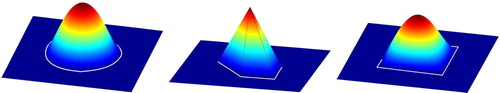
(1) Note that in general we do not assume that $Q_l={\mathrm{\Pi }}_l,$, i.e. we do not reconstruct the inhomogeneity of the solid on an a priory given set of subdomains. (2) The supports of the functions ${\psi }_l\left(x\right)$ may in fact differ from the parallelepipeds ${\mathrm{\Pi }}_l.$ Thus, one can consider not only piecewise constants but a much wider approximating classes of functions (see Figure 1).

Figure 1. Plots of various approximating functions ${\psi }_l(x_1,x_2,x_3)$ in Q (the variable $x_3$ is fixed).

Theorem 3.5

Let (23) $k_0>\frac{{\pi }^2{n}^3}{2d},d=\underset{1\le i\le 3}{min}|b_i-a_i|.$(23) Then equation (24) ${\int }_{Q}G(x,y)J\left(y\right)\mathrm{d}y=u_s\left(x\right),x\in D,\overline{D}\cap \overline{Q}=\mathrm{\varnothing },u_s\in C^{\mathrm{\infty }}\left(\overline{D}\right)$(24) has at most one solution $J\in S\left({\mathcal{Q}}_n\right).$ In addition, Equation (24(24) ${\int }_{Q}G(x,y)J\left(y\right)\mathrm{d}y=u_s\left(x\right),x\in D,\overline{D}\cap \overline{Q}=\mathrm{\varnothing },u_s\in C^{\mathrm{\infty }}\left(\overline{D}\right)$(24) ) has at most one solution $J\in S\left({\mathcal{Q}}_n\right)$ for every $n\in \mathbb{N}$ and for any wave number $k_0>0,$ with the possible exception of finite number of its values.

Let us assume that the right-hand side $u_s\left(x\right)$ of (24(24) ${\int }_{Q}G(x,y)J\left(y\right)\mathrm{d}y=u_s\left(x\right),x\in D,\overline{D}\cap \overline{Q}=\mathrm{\varnothing },u_s\in C^{\mathrm{\infty }}\left(\overline{D}\right)$(24) ) belongs to the class $\mathcal{A}S\left({\mathcal{Q}}_n\right).$ Then the operator of the left hand side of (24(24) ${\int }_{Q}G(x,y)J\left(y\right)\mathrm{d}y=u_s\left(x\right),x\in D,\overline{D}\cap \overline{Q}=\mathrm{\varnothing },u_s\in C^{\mathrm{\infty }}\left(\overline{D}\right)$(24) ) can be treated as a mapping in finite-dimensional spaces. It results from Theorem 3.5 that such a mapping is continuously invertible. Thus, we arrive at

Theorem 3.6

If condition (23(23) $k_0>\frac{{\pi }^2{n}^3}{2d},d=\underset{1\le i\le 3}{min}|b_i-a_i|.$(23) ) is satisfied, then for any $u_s\left(x\right)\in \mathcal{A}S\left({\mathcal{Q}}_n\right)$ there exists a unique solution of Equation (24(24) ${\int }_{Q}G(x,y)J\left(y\right)\mathrm{d}y=u_s\left(x\right),x\in D,\overline{D}\cap \overline{Q}=\mathrm{\varnothing },u_s\in C^{\mathrm{\infty }}\left(\overline{D}\right)$(24) ).

4. Numerical simulation

To illustrate the proposed method, we numerically study a series of test inverse problems assuming that Q is an inhomogeneous parallelepiped whose contrast function is everywhere non-zero. More precisely, condition (13(13) $|k\left(x\right)|\ge \tilde{k}>k_0$(13) ) is always satisfied.

The approach for solving a test problem is as follows. First, we consider the cube Q with a function $k\left(x\right),$ $x\in \overline{Q},$ which represents the exact solution to the inverse problem. Second, for the given function $k\left(x\right)$ we find a unique solution $u\left(x\right),x\in Q,$ of the forward scattering problem which is then used for determining the simulated total field $u\left(x\right),x\in D,$ of the inverse scattering problem (see relation (9(9) $\begin{array}{rl}& u\left(x\right)=u_0\left(x\right)+{\int }_Q\left(k^2\right(y)-k_0^2)G(x,y)u\left(y\right)dy,x\in {\mathbb{R}}^3\setminus (Q\cup \{x_0\left\}\right).\end{array}$(9) )).

Given the incident wave $u_0$ and the simulated total field u in D, we find a solution J to (16(16) $\begin{array}{rl}& {\int }_{Q}G(x,y)J\left(y\right)\mathrm{d}y=u\left(x\right)-u_0\left(x\right)=u_s\left(x\right),x\in D,\end{array}$(16) ). In the present work, we consider the classes $S\left({\mathcal{Q}}_n\right)$ of piecewise-constant functions $J\left(x\right)=\sum _l{J}_l{\psi }_l\left(x\right)$. Here ${\psi }_l\left(x\right)$ are the characteristic functions of the balls $B_{r_n}\left(c_l\right)$ of radius $r_n$ centred at points $c_l\in Q.$ The radius $r_n$ is fixed for any given partition and the points $c_l$ are chosen as to satisfy conditions (1)–(4) on page 15. Actually, we define $c_l$ as the centres of the rectangles ${\mathrm{\Pi }}_l$ defined by (18(18) $x_{1,l_1}=a_1+\frac{b_1-a_1}{n}{l}_1,x_{2,l_2}=a_2+\frac{b_2-a_2}{n}{l}_2,x_{3,l_3}=a_3+\frac{b_3-a_3}{n}{l}_3,0\le l_k\le n,$(18) ),(19(19) ${\mathrm{\Pi }}_l={\mathrm{\Pi }}_{l_1{l}_2{l}_3}=\{x:x_{k,l_k}<x_k<x_{k,l_k+1}\},k=1,2,3,0\le l_k\le n-1,$(19) ). Finally, using formula (17(17) $\begin{array}{rl}& \frac{J\left(x\right)}{k^2\left(x\right)-k_0^2}-{\int }_{Q}G(x,y)J\left(y\right)\mathrm{d}y=u_0\left(x\right),x\in Q.\end{array}$(17) ), we recover the sought-for function $k\left(x\right)$.

We use collocation method for approximate solving equation (16(16) $\begin{array}{rl}& {\int }_{Q}G(x,y)J\left(y\right)\mathrm{d}y=u\left(x\right)-u_0\left(x\right)=u_s\left(x\right),x\in D,\end{array}$(16) ). To this end, we define sets of collocation nodes $x_k$ in the domain D, where the total field is given. Approximate solutions are sought in the form (22(22) $J\left(x\right)=\sum _l{J}_l{\psi }_l\left(x\right),$(22) ) with the characteristic functions ${\psi }_l.$ To obtain a unique approximate solution we require that the number of equations be equal to the number N of unknown coefficients $J_l.$ This implies that the number of collocation points representing the receivers' positions (or points of the field measuring) should be equal to N. We use the central rectangles rule for calculating the integrals of the left hand side of (24(24) ${\int }_{Q}G(x,y)J\left(y\right)\mathrm{d}y=u_s\left(x\right),x\in D,\overline{D}\cap \overline{Q}=\mathrm{\varnothing },u_s\in C^{\mathrm{\infty }}\left(\overline{D}\right)$(24) ). Since the integration domains are ${\mathrm{\Pi }}_l\subset Q,$ the points $x_k\in D$ and $\overline{Q}\cap \overline{D}=\mathrm{\varnothing },$ then the kernel G is smooth. Consequently, the rectangle rule provides sufficient accuracy. In practice, we apply the midpoint rule with at most $8^3$ terms in the quadrature.

Application of the collocation method and non-iterative procedures for finding solutions makes the TSM a relatively fast method which doesn't require supercomputing or distributed computing. In the carried out experiments which took from 1 to 18 min, a PC with the CoreI5–8300h processor with the clock speed 3.9 GHz was used. The random-access memory (RAM) requirements depend primarily on the number of the sought-for coefficients $J_l.$ In the tested implementation of the algorithm, the required RAM varied from 0.15 to 1.5 GB.

Below, we discuss results of numerical solving the inverse problem as well as the comparison of the exact solution of the inverse problem and the approximate ones.

We take the cube $Q=[-0.075,0.075{]}^3$ with a side of 15 cm. The incident wave is defined by (5(5) $u_0\left(x\right)=\frac{{\mathrm{e}}^{\mathrm{i}{k}_0|x-x_0|}}{4\pi |x-x_0|},x_0\notin \overline{Q},$(5) ), where the source is located at the point $x_0=(0,0,0.15),$ the wave frequency varies within the range of 25–27 GHz. We consider the domain $D=D_1\cup D_2,$ where $D_1$ and $D_2$ are located on the opposite sides of Q: $D_1=(-0.09,0.08)\times (-0.075,0.075)\times (-0.075,0.075)$ and $D_1=(0.08,0.09)\times (-0.075,0.075)\times (-0.075,0.075).$ The mesh sizes in Q and D vary from 0.5 to 1.5 cm depending on n (see formulas (18(18) $x_{1,l_1}=a_1+\frac{b_1-a_1}{n}{l}_1,x_{2,l_2}=a_2+\frac{b_2-a_2}{n}{l}_2,x_{3,l_3}=a_3+\frac{b_3-a_3}{n}{l}_3,0\le l_k\le n,$(18) ) and (19(19) ${\mathrm{\Pi }}_l={\mathrm{\Pi }}_{l_1{l}_2{l}_3}=\{x:x_{k,l_k}<x_k<x_{k,l_k+1}\},k=1,2,3,0\le l_k\le n-1,$(19) )).

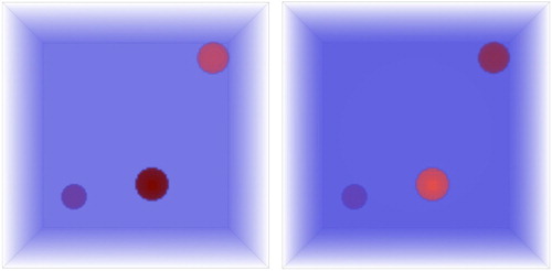
In this work, we consider the case of three ball-shaped inclusions: the inhomogeneity of the solid is described by a piecewise-continuous complex-valued function $k\left(x\right)$ which is equal to 20 + 10i except for three spherical subdomains, where $\mathrm{\Re }k\left(x\right)$ varies from 33 to 38 and $\mathrm{\Im }k\left(x\right)$ is chosen within the segment $[17;18].$ Figure 2 shows the real and the imaginary parts of the exact solution to the test problem.

Figure 2. The real (left) and the imaginary (right) parts of the exact solution of the model inverse problem with noiseless data: $\mathbf{n}\mathbf{l}=0\mathrm{\%}.$ The wave frequency is 27 GHz.

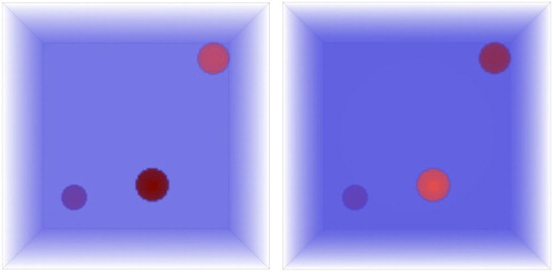
The next set of figures is presented for understanding the dependance of approximate solutions' accuracy on the amount of noise in the data. Note that, given pure simulated data (undisturbed field u in the domain D), we obtain very accurate solutions which can hardly be distinguished from the exact ones (see Figure 3). We simulate noising of the data in the following way: we first solve the forward problem with ‘pure’ data; then we evaluate the field in the region D by formula (9(9) $\begin{array}{rl}& u\left(x\right)=u_0\left(x\right)+{\int }_Q\left(k^2\right(y)-k_0^2)G(x,y)u\left(y\right)dy,x\in {\mathbb{R}}^3\setminus (Q\cup \{x_0\left\}\right).\end{array}$(9) ) adding random noise to the density $u\left(x\right),x\in Q,$ of the volume potential. More precisely, we set $u_s\left(x\right)={\int }_Q\left(k^2\right(y)-k_0^2)G(x,y)\tilde{u}\left(y\right)dy,$ where the $\tilde{u}\left(y\right)=(1+rand(-\nu ,\nu \left)\right)u\left(y\right).$ Here $rand(-\nu ,\nu )$ returns a random real from the interval $(-\nu ,\nu ),$ and ν is the noise level. So, if $\nu =0.05$ we say that the data is noisy with the noise level $\mathbf{n}\mathbf{l}=5\mathrm{\%}.$ Thus, a good simulation of perturbed near field data $u_s\left(x\right),x\in D,$ is obtained. Figure 4 demonstrates approximate solutions of the inverse problem with disturbed data showing noisy background and numerous artefacts. The noise level denoted by $\mathbf{n}\mathbf{l}$ ranges from $0.1\mathrm{\%}$ to $0.5\mathrm{\%}$ with respect to the amplitude of the noiseless field.

Figure 3. The real (left) and the imaginary (right) parts of the approximate solution of the model inverse problem with noiseless data: $\mathbf{n}\mathbf{l}=0\mathrm{\%}.$ The wave frequency is 27 GHz.

We use the same method for erasing artefacts and more accurate detection of true inhomogeneities as in [21]. The method is in two procedures.

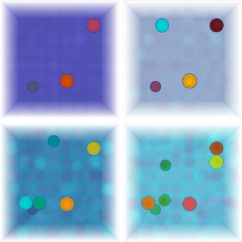
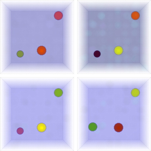
Figure 4. The real part of approximate solution of the model inverse problem with noisy near field data. The values of the noise level are $\mathbf{n}\mathbf{l}=0.1\mathrm{\%}$, $\mathbf{n}\mathbf{l}=0.25\mathrm{\%}$, $\mathbf{n}\mathbf{l}=0.4\mathrm{\%}$, and $\mathbf{n}\mathbf{l}=0.5\mathrm{\%}$. The wave frequency is 27 GHz.

The first preprocessing procedure is used for filtering noisy near field data in the domain D. We take a collocation node $x_k\in D$ and consider its small vicinity $U_{x_k}$ with diameter $d\left(U_{x_k}\right)=\delta ,$ where δ is the minimal distance from $x_k$ to other collocation points. We calculate the average value $u_s^{av}$ in $U_{x_k}$ using (9(9) $\begin{array}{rl}& u\left(x\right)=u_0\left(x\right)+{\int }_Q\left(k^2\right(y)-k_0^2)G(x,y)u\left(y\right)dy,x\in {\mathbb{R}}^3\setminus (Q\cup \{x_0\left\}\right).\end{array}$(9) ) and make a comparison between $u_s^{av}$ and the given value $u_s\left(x_k\right).$ If $|u_s^{av}-u_s\left(x_k\right)|$ is not within 5% of the value $|u_s^{av}|$ then we set $u_s\left(x_k\right)=u_s^{av}$ in the collocation method. Otherwise, the given value $u_s\left(x_k\right)$ is used. The same averaging procedure can also be applied to experimentally obtained data.

The second is the postprocessing procedure (refinement of approximate solutions). We make a series of several experiments and find approximate solutions at three various frequencies (see Figure 5). Then we compare the approximate solutions $k^{\left(1\right)}\left(x\right),$ $k^{\left(2\right)}\left(x\right)$ and $k^{\left(3\right)}\left(x\right)$ at the points of subdomains ${\mathrm{\Pi }}_l$ assuming that the true homogeneities are at the same positions of the inhomogeneity domain, and the artefacts change their location or even disappear. The solution $k^{\left(1\right)}\left(x\right)$ corresponding to the original value of the wave frequency is the one to be refined, whereas $k^{\left(2\right)}\left(x\right)$ and $k^{\left(3\right)}\left(x\right)$ are supplementary solutions. The further analysis is as follows: if the difference between these values is less than 5% of the average $k_l^{av}$ and is within 10% of the background values then we say that $k^{\left(1\right)}\left(x\right)$ represents the wave number of the background. Otherwise we set $k\left(x\right):=\left(k^{\left(1\right)}\right(x)+k^{\left(2\right)}(x)+k^{\left(3\right)}(x\left)\right)/3$ and call it the wave number of the sought-for inhomogeneity. In addition, a background levelling can be carried out in those grid cells ${\mathrm{\Pi }}_l^{bg}$ that are treated as background subdomains. This procedure is a kind of averaging the values at background cells (a detailed description is given in [21]). The result of solution's refinement is presented in Figure 6.

Figure 5. Approximate solutions of the model inverse problem with noisy near field data obtained at three wave frequencies: 25, 26 and 27 GHz. The noise level is $\mathbf{n}\mathbf{l}=0.25\mathrm{\%}$.

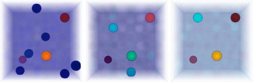
Figure 7 demonstrates the real part of the approximate solutions refined by the pre- and postprocessing procedures.

Figure 6. The refined approximate solution of the model problem with noisy near field data with $\mathbf{n}\mathbf{l}=0.25\mathrm{\%}.$

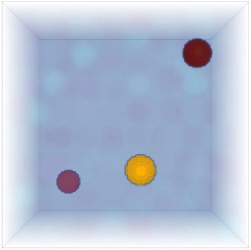
Figure 7. The real part of refined approximate solutions of the model inverse problem with noisy near field data. The values of the noise level are $\mathbf{n}\mathbf{l}=0.1\mathrm{\%}$, $\mathbf{n}\mathbf{l}=0.25\mathrm{\%}$, $\mathbf{n}\mathbf{l}=0.4\mathrm{\%}$, and $\mathbf{n}\mathbf{l}=0.5\mathrm{\%}.$

Thus, the experiments show high efficiency of the described methods if the noise level is less than 0.5% of the pure data.

5. Proofs of the theorems

Proof of Theorem 2.4.

Proof of Theorem 2.4

From the definition of the incident wave in the considered statement of the problem it follows that $u_0\in C^{\mathrm{\infty }}({\mathbb{R}}^3\setminus \{x_0\left\}\right)$.

The extension of a solution $u\left(x\right)$ to the integral equation is infinitely differentiable outside the solid since the smoothness of the integral operator kernel at each $x\notin \overline{Q}$.

Now we consider equation (8(8) $\begin{array}{rl}& u\left(x\right)-{\int }_Q\left(k^2\right(y)-k_0^2)G(x,y)u\left(y\right)\mathrm{d}y=u_0\left(x\right),x\in Q,\end{array}$(8) ). For each index l, we have (25) $\begin{array}{rl}& u\left(x\right)-{\int }_{Q_l}\left(k_l^2\right(y)-k_0^2)G(x,y)u\left(y\right)\mathrm{d}y\\ & =\sum _{j\ne l}{\int }_{Q_j}\left(k_j^2\right(y)-k_0^2)G(x,y)u\left(y\right)\mathrm{d}y+u_0\left(x\right),x\in Q_l.\end{array}$(25) The right-hand side of the equation is infinitely smooth in the open domain $Q_l$ since, for any $j\ne l,$ we have $G(x,y)\in C^{\mathrm{\infty }}(Q_j\times Q_l)$.

The inclusion $u\left(x\right)\in L_2\left(Q\right)$ implies $u\in H^2\left(Q\right)$ and, consequently, $u\in C^{\alpha }\left(\overline{Q}\right)$ for all $0<\alpha <1/2.$ Then $Au\in C^1\left({\mathbb{R}}^3\right)$ [26]. It follows from the latter that $u\in C^1({\mathbb{R}}^3\setminus \{x_0\left\}\right)$ which also results in the energy finiteness condition $u\in H_{\mathrm{l}\mathrm{o}\mathrm{c}}^1({\mathbb{R}}^3\setminus \{x_0\left\}\right)$.

It suffices to prove that $u\in C^2\left(Q_l\right)$ for any l. Write the following equality for u according to (25(25) $\begin{array}{rl}& u\left(x\right)-{\int }_{Q_l}\left(k_l^2\right(y)-k_0^2)G(x,y)u\left(y\right)\mathrm{d}y\\ & =\sum _{j\ne l}{\int }_{Q_j}\left(k_j^2\right(y)-k_0^2)G(x,y)u\left(y\right)\mathrm{d}y+u_0\left(x\right),x\in Q_l.\end{array}$(25) ): $u\left(x\right)={\int }_{Q_l}\left(k_l^2\right(y)-k_0^2)G(x,y)u\left(y\right)\mathrm{d}y+w\left(x\right)=v\left(x\right)+w\left(x\right),x\in Q_l,$ where $w\in C^{\mathrm{\infty }}\left(Q_l\right)$.

Let $x_0\in Q_l$ be an arbitrary inner point of the lth sub-domain such that $d=\underset{x\in \mathrm{\partial }{Q}_l}{min}|x_0-x|>0.$ Introduce the cut-off function $c\in C^{\mathrm{\infty }}\left(Q_l\right):$ (26) $c\left(y\right)=\left\{\begin{array}{ll}1& \mathrm{f}\mathrm{o}\mathrm{r}y\in B=B_{d/4}\left(x_0\right),\\ 0& \mathrm{f}\mathrm{o}\mathrm{r}y\in B=Q_l\setminus B_{3d/4}\left(x_0\right).\end{array}\right.$(26) We represent v in the form (27) $\begin{array}{rl}v\left(x\right)=v_1\left(x\right)+v_2\left(x\right)& ={\int }_{Q_l}\left(k_l^2\right(y)-k_0^2)G(x,y)u\left(y\right)c\left(y\right)\mathrm{d}y\\ & +{\int }_{Q_l\setminus B}\left(k_l^2\right(y)-k_0^2)G(x,y)u\left(y\right)(1-c(y\left)\right)\mathrm{d}y.\end{array}$(27) Since the kernel in the second term is smooth, we obtain $v_2\in C^{\mathrm{\infty }}\left(B\right)$.

Note that $u\in C^{\alpha }\left(Q_l\right),$ $c\in C_0^{\mathrm{\infty }}\left(Q_l\right)$ and, consequently, (28) $\left(k_l^2\right(y)-k_0^2)u\left(y\right)c\left(y\right)\in C_0^{\alpha }\left({\mathbb{R}}^3\right).$(28)

Using the properties of the volume potential (for details, see [15]), we obtain from the latter that $v_1\in C^{2,\alpha }\left({\mathbb{R}}^3\right)$.

Thus, a solution $u\left(x\right)$ is twice differentiable in a vicinity of each point $x_0\in Q_l,$ i.e. $u\in C^2\left(Q_l\right)$.

Proof of Theorem 2.5.

Proof of Theorem 2.5

(1) The former part of the theorem follows from the derivation of the integral equation (8(8) $\begin{array}{rl}& u\left(x\right)-{\int }_Q\left(k^2\right(y)-k_0^2)G(x,y)u\left(y\right)\mathrm{d}y=u_0\left(x\right),x\in Q,\end{array}$(8) ).

(2) Let u be a solution to (8(8) $\begin{array}{rl}& u\left(x\right)-{\int }_Q\left(k^2\right(y)-k_0^2)G(x,y)u\left(y\right)\mathrm{d}y=u_0\left(x\right),x\in Q,\end{array}$(8) ) with $u_0\in C^{\mathrm{\infty }}({\mathbb{R}}^3\setminus \{x_0\left\}\right)$. The definition of u in terms of a volume potential together with smoothness of the term $u_0$ in ${\mathbb{R}}^3\setminus \left\{x_0\right\}$ imply that u is a solution to the Helmholtz equation in the domains $Q_l$ and ${\mathbb{R}}^3\setminus \left(\right\{x_0\}\cup \overline{Q})$.

The scattered field $u_s\left(x\right)={\int }_Q\left(k^2\right(y)-k_0^2)G(x,y)u\left(y\right)\mathrm{d}y$ satisfies the radiation condition, whereas the transmission conditions are fulfilled since the inclusion $u\in C^1({\mathbb{R}}^3\setminus \{x_0\left\}\right)$ shown in Theorem 2.4. Note that the equality $\mathrm{\partial }u/\mathrm{\partial }\mathbf{n}=0$ cannot be formulated on the edges of the sub-domains $Q_l$.

Proof of Theorem 3.5.

Proof of Theorem 3.5

(1) Consider the homogeneous equation ${\int }_{Q}G(x,y)J\left(y\right)\mathrm{d}y=0,x\in D.$

Introduce the volume potential (29) $v\left(x\right)={\int }_{Q}G(x,y)J\left(y\right)\mathrm{d}y,x\in {\mathbb{R}}^3.$(29)

Since $J\left(x\right)$ is a continuous (or piecewise continuous and bounded) function, then $v\left(x\right)\in C^1\left({\mathbb{R}}^3\right).$ As a result, the transmission conditions $v{|}_{\mathrm{\partial }{\mathrm{\Pi }}_l}=\frac{\mathrm{\partial }v}{\mathrm{\partial }\mathbf{n}}{|}_{\mathrm{\partial }{\mathrm{\Pi }}_l^{\prime }}=0$ hold on the boundaries of ${\mathrm{\Pi }}_l.$

Moreover, the inclusions $v\in C^2\left({\mathrm{\Pi }}_l\right)$ are valid. Consequently, the Helmholtz equation $(\mathrm{△}+k_0^2)v\left(x\right)=-J_l,x\in {\mathrm{\Pi }}_l$ holds at the inner points $x\in {\mathrm{\Pi }}_l$ (in the classical sense).

Outside $\overline{Q},$ we obtain $(\mathrm{△}+k_0^2)v\left(x\right)=0$ and $v\in C^{\mathrm{\infty }}({\mathbb{R}}^3\setminus \overline{Q}).$

By the assumption of the theorem, the function v is equal to zero in the domain $D\subset {\mathbb{R}}^3\setminus \overline{Q}$. Then, applying the unique continuation principle [15], we derive that $v\equiv 0$ everywhere in ${\mathbb{R}}^3\setminus \overline{Q}$.

It follows from the inclusion $v\left(x\right)\in C^1\left({\mathbb{R}}^3\right)$ that the relation (30) $v{|}_{\mathrm{\partial }Q}=\frac{\mathrm{\partial }v}{\mathrm{\partial }\mathbf{n}}{|}_{\mathrm{\partial }{Q}^{\prime }}=0$(30) holds.

(2) Consider the fundamental solution $\overline{G}(x,y)={\mathrm{e}}^{-\mathrm{i}{k}_0|x-y|}/\left(4\pi |x-y|\right)$ of the Helmholtz equation. Applying the second Green formula to the functions v and $\overline{G}$ in the domains ${\mathrm{\Pi }}_l,$ taking into account the homogeneous boundary conditions (30(30) $v{|}_{\mathrm{\partial }Q}=\frac{\mathrm{\partial }v}{\mathrm{\partial }\mathbf{n}}{|}_{\mathrm{\partial }{Q}^{\prime }}=0$(30) ) and the transmission conditions on $\mathrm{\partial }{\mathrm{\Pi }}_l$ for the function v, we find $\begin{array}{rl}0& ={\int }_{\mathrm{\partial }Q}\left(v\left(y\right)\frac{\mathrm{\partial }}{\mathrm{\partial }\mathbf{n}}\overline{G}(x,y)-\overline{G}(x,y)\frac{\mathrm{\partial }}{\mathrm{\partial }\mathbf{n}}v\left(y\right)\right)\mathrm{d}{s}_y\\ & =\sum _l{\int }_{\mathrm{\partial }{\mathrm{\Pi }}_l}\left(v\left(y\right)\frac{\mathrm{\partial }}{\mathrm{\partial }\mathbf{n}}\overline{G}(x,y)-\overline{G}(x,y)\frac{\mathrm{\partial }}{\mathrm{\partial }\mathbf{n}}v\left(y\right)\right)\mathrm{d}{s}_y\\ & =\sum _l{\int }_{{\mathrm{\Pi }}_l}\left(v\left(y\right){\mathrm{△}}_y\overline{G}(x,y)-\overline{G}(x,y){\mathrm{△}}_{y}v\left(y\right)\right)\mathrm{d}y\\ & =\sum _{l\ne l_0}{\int }_{{\mathrm{\Pi }}_l}(-k_0^{2}v\left(y\right)\overline{G}(x,y)-\overline{G}(x,y){\mathrm{△}}_{y}v\left(y\right))\mathrm{d}y\\ & +{\int }_{{\mathrm{\Pi }}_{l_0}}(-k_0^{2}v\left(y\right)\overline{G}(x,y)-\delta (x-y)v\left(y\right)-\overline{G}(x,y){\mathrm{△}}_{y}v\left(y\right))\mathrm{d}y\\ & =-v\left(x\right)+\sum _l{J}_l{\int }_{{\mathrm{\Pi }}_l}\overline{G}(x,y)\mathrm{d}y,x\in {\mathrm{\Pi }}_{l_0}.\end{array}$ It follows from the latter that (31) $v\left(x\right)={\int }_Q\overline{G}(x,y)J\left(y\right)\mathrm{d}y,x\in Q.$(31)

Subtracting (31(31) $v\left(x\right)={\int }_Q\overline{G}(x,y)J\left(y\right)\mathrm{d}y,x\in Q.$(31) ) from (29(29) $v\left(x\right)={\int }_{Q}G(x,y)J\left(y\right)\mathrm{d}y,x\in {\mathbb{R}}^3.$(29) ), we deduce $w\left(x\right)={\int }_Q\frac{\sin (k_0|x-y|)}{4\pi |x-y|}J\left(y\right)\mathrm{d}y={\int }_Q{G}_0(x,y)J\left(y\right)\mathrm{d}y\equiv 0,x\in Q.$

Note that the kernel $G_0(x,y)=G_0(|x-y|)$ is an analytic function which satisfies the homogeneous Helmholtz equation. Since the repeated differentiation is valid for $w\left(x\right),$ then $(\mathrm{△}+k_0^2)w\left(x\right)={\int }_Q({\mathrm{△}}_x+k_0^2)G_0(x,y)J\left(y\right)\mathrm{d}y=0.$ Thus, the function $w\in C^2\left({\mathbb{R}}^3\right)$ is a classical solution to the Helmholtz equation in ${\mathbb{R}}^3$ and is equal to zero in Q. The unique continuation principle implies that $w\equiv 0$ in ${\mathbb{R}}^3$.

(3) Thus, $w\equiv 0$ in ${\mathbb{R}}^3$. Then everywhere in ${\mathbb{R}}^3,$ the Fourier transform $Fw\left(\xi \right)$ identically equals zero. Since ${\mathrm{\Pi }}_l={\mathrm{\Pi }}_0+{\mathbf{r}}_l$ for all $l$, then the function $w\left(x\right)$ can now be represented as follows $w\left(x\right)=\sum _l{J}_l{\int }_{{\mathrm{\Pi }}_0+{\mathbf{r}}_l}{G}_0(|x-y|)\mathrm{d}x=\sum _l{J}_l{\int }_{{\mathrm{\Pi }}_0}{G}_0(|x-y-{\mathbf{r}}_l|)\mathrm{d}x.$

Evaluating the Fourier transform of w and taking into account the latter relation, we find $\begin{array}{rl}Fw& =\sum _l{J}_{l}F(G_0(|x-{\mathbf{r}}_l|)\ast {\psi }_0\left(x\right))\\ & =\sum _l{J}_{l}F(G_0(|x-{\mathbf{r}}_l|))F({\psi }_0\left(x\right))=F{\psi }_0\left(\xi \right)F{G}_0\left(\xi \right)\sum _l{J}_l{\mathrm{e}}^{\mathrm{i}{\mathbf{r}}_l\cdot \xi }\\ & =F{\psi }_0\left(\xi \right)\cdot \delta (|\xi |-k_0)\cdot \sum _l{J}_l{\mathrm{e}}^{\mathrm{i}{\mathbf{r}}_l\cdot \xi }.\end{array}$

The properties of the functions ${\psi }_l$ (see page 8) imply that the relation $Fw\equiv 0$ can be reduced to the equality $\sum _l{J}_l{\mathrm{e}}^{\mathrm{i}{\mathbf{r}}_l\cdot \xi }\equiv 0$ on the centred sphere $S_{k_0}$ of the radius $k_0$.

(4) Let us show that the functions ${\mathrm{e}}^{\mathrm{i}{r}_l\cdot \xi }$ are linearly independent on the sphere $S_{k_0}.$ To this end we will prove that the corresponding Gram matrix Γ is nonsingular.

We denote a unit sphere in ${\mathbb{R}}^n$ ($n\ge 2$) by $S^{n-1}.$ For an arbitrary matrix element ${\mathrm{\Gamma }}_{l{l}^{\prime }}$ we deduce (32) $\begin{array}{rl}{\mathrm{\Gamma }}_{l{l}^{\prime }}& ={\int }_{S_{k_0}}{\mathrm{e}}^{\mathrm{i}{\mathbf{r}}_l\cdot \xi }{\mathrm{e}}^{-\mathrm{i}{\mathbf{r}}_{l^{\prime }}\cdot \xi }\mathrm{d}{s}_{\xi }=k_0^2{\int }_{S^2}{\mathrm{e}}^{\mathrm{i}{k}_0({\mathbf{r}}_l-{\mathbf{r}}_{l^{\prime }})\cdot \xi }\mathrm{d}{s}_{\xi }=k_0^2{\int }_{S^2}{\mathrm{e}}^{\mathrm{i}{k}_0{\mathbf{r}}_{l{l}^{\prime }}\cdot \xi }\mathrm{d}{s}_{\xi }\\ & =k_0^2{\int }_{S^2}{\mathrm{e}}^{\mathrm{i}{k}_0|{\mathbf{r}}_{l{l}^{\prime }}|{\mathrm{\Pi }}_{l{l}^{\prime }}\cdot \xi }\mathrm{d}{s}_{\xi }=2\pi k_0^2{\int }_{-1}^1{\mathrm{e}}^{\mathrm{i}{k}_0|{\mathbf{r}}_{l{l}^{\prime }}|t}\mathrm{d}t.\end{array}$(32) In the above evaluation, the integrals ${\int }_{S^{n-1}}f(\theta \cdot \xi )\mathrm{d}{s}_{\xi }$ over the unit centred sphere $S^{n-1}$ do not depend on the variable $\theta \in S^{n-1}$ and, consequently, can be presented [27] as below: ${\int }_{S^{n-1}}f(\theta \cdot \xi )\mathrm{d}{s}_{\xi }=|S^{n-2}|{\int }_{-1}^{1}f\left(t\right)(1-t^2{)}^{(n-3)/2}\mathrm{d}t.$ From (32(32) $\begin{array}{rl}{\mathrm{\Gamma }}_{l{l}^{\prime }}& ={\int }_{S_{k_0}}{\mathrm{e}}^{\mathrm{i}{\mathbf{r}}_l\cdot \xi }{\mathrm{e}}^{-\mathrm{i}{\mathbf{r}}_{l^{\prime }}\cdot \xi }\mathrm{d}{s}_{\xi }=k_0^2{\int }_{S^2}{\mathrm{e}}^{\mathrm{i}{k}_0({\mathbf{r}}_l-{\mathbf{r}}_{l^{\prime }})\cdot \xi }\mathrm{d}{s}_{\xi }=k_0^2{\int }_{S^2}{\mathrm{e}}^{\mathrm{i}{k}_0{\mathbf{r}}_{l{l}^{\prime }}\cdot \xi }\mathrm{d}{s}_{\xi }\\ & =k_0^2{\int }_{S^2}{\mathrm{e}}^{\mathrm{i}{k}_0|{\mathbf{r}}_{l{l}^{\prime }}|{\mathrm{\Pi }}_{l{l}^{\prime }}\cdot \xi }\mathrm{d}{s}_{\xi }=2\pi k_0^2{\int }_{-1}^1{\mathrm{e}}^{\mathrm{i}{k}_0|{\mathbf{r}}_{l{l}^{\prime }}|t}\mathrm{d}t.\end{array}$(32) ) it follows that ${\mathrm{\Gamma }}_{l{l}^{\prime }}=\left\{\begin{array}{ll}4\pi k_0\frac{\sin \left(k_0|r_{l{l}^{\prime }}|\right)}{|r_{l{l}^{\prime }}|}& \mathrm{f}\mathrm{o}\mathrm{r}l\ne l^{\prime },\\ 4\pi k_0^2& \mathrm{f}\mathrm{o}\mathrm{r}l=l^{\prime }.\end{array}\right.$

(5) Represent Γ via sum $\mathrm{\Gamma }=4\pi k_0(k_0\tilde{I}+\tilde{\mathrm{\Gamma }}),$ where $\tilde{I}$ is the unit matrix, and obtain the estimate (33) $\parallel \tilde{\mathrm{\Gamma }}{\parallel }_{\mathrm{\infty }}=\underset{l}{max}\sum _{l^{\prime }}|{\tilde{\mathrm{\Gamma }}}_{l{l}^{\prime }}|\le \frac{{\pi }^2{n}^3}{2h}.$(33)

Fix the row index $l^{\prime }=(0,0,0)$ and define $h=min\{h_1,h_2,h_3\}$: $\begin{array}{rl}\sum _{l\ne l^{\prime }}|{\tilde{\mathrm{\Gamma }}}_{l{l}^{\prime }}|& =\sum _{l\ne l^{\prime }}\frac{1}{|r_{l{l}^{\prime }}|}=\sum _{(i_1,i_2,i_3)=(0,0,1)}^{(n-1,n-1,n-1)}\frac{1}{\sqrt{(i_1{h}_1{)}^2+(i_2{h}_2{)}^2+(i_3{h}_3{)}^2}}\\ & <\frac{6}{h}+\frac{1}{h}\sum _{(i_1,i_2,i_3)=(1,1,1)}^{(n,n,n)}\frac{1}{\sqrt{(i_1{)}^2+(i_2{)}^2+(i_3{)}^2}}\\ & \le \frac{1}{h}\left(6+2{\int }_1^n\frac{\mathrm{d}x}{|x|}\right)\le \frac{1}{h}\left(6+0.5{\int }_{1<|x|<n}\frac{\mathrm{d}x}{|x|}\right)\\ & =\frac{1}{h}\left(6+{\pi }^2{\int }_1^n\frac{r^2}{r}\mathrm{d}r\right)<\frac{{\pi }^2}{2}\frac{n^2}{h}\le \frac{{\pi }^2{n}^3}{2d}.\end{array}$

The estimate (33(33) $\parallel \tilde{\mathrm{\Gamma }}{\parallel }_{\mathrm{\infty }}=\underset{l}{max}\sum _{l^{\prime }}|{\tilde{\mathrm{\Gamma }}}_{l{l}^{\prime }}|\le \frac{{\pi }^2{n}^3}{2h}.$(33) ) implies that the determinant of the Gram matrix is non-zero, since its diagonal element dominate at sufficiently large n.

Note that the determinant $det\mathrm{\Gamma }$ of the Gram matrix depends analytically on $k_0$ (in terms of functions of a complex variable) for arbitrary $n\in \mathbb{N}.$ Hence, $det\mathrm{\Gamma }\left(k_0\right)$ can have a finite number of zeros within any bounded segment $k_0\in (0,k_0^{\prime }).$ Thus, Equation (24(24) ${\int }_{Q}G(x,y)J\left(y\right)\mathrm{d}y=u_s\left(x\right),x\in D,\overline{D}\cap \overline{Q}=\mathrm{\varnothing },u_s\in C^{\mathrm{\infty }}\left(\overline{D}\right)$(24) ) has a unique solution from the class $S\left({\mathcal{Q}}_n\right)$ for every $n\in \mathbb{N}$ and for any wave number $k_0>0,$ with the possible exception of finite number of its values.

The proof is complete.

Conclusion

We have theoretically justified and implemented the two-step method for solving the three-dimensional problem of recovering a refractive index of a volumetric scatterer Q using noisy near field data. The index can be described by a continuous or piecewise Hölder function that may have discontinuities on boundaries $\mathrm{\partial }{Q}_l$ of several subdomains $Q_l$ of Q. The proposed non-iterative method involves solving a linear source-type integral equation. We proved uniqueness of a solution to such an equation in the class of linear combinations of functions with compact supports ${\mathrm{\Pi }}_l\ne Q_l$. An efficient two-stage refinement procedure is proposed and implemented. The procedure allows to obtain solutions to the problem with noisy near field data, where the noise level is within $0.5\mathrm{\%}$.

Disclosure statement

No potential conflict of interest was reported by the author(s).

ORCID

M. Yu. Medvedik  http://orcid.org/0000-0003-4066-1818

Yu. G. Smirnov  http://orcid.org/0000-0001-9040-628X

A. A. Tsupak  http://orcid.org/0000-0002-4462-4697

Additional information

Funding

This work was supported by the Ministry of Education and Science of the Russian Federation [agreement no. 1.894.2017/4.6] and Russian Foundation for Basic Research [grant number 18-01-00219 A].

References

- Brown BM, Marlett M, Reyes JM. Uniqueness for an inverse problem in electromagnetism with partial data. J Differ Equations. 2016;260:6525–6547. doi: 10.1016/j.jde.2016.01.002
- Ammari H, Kang H. Reconstruction of small inhomogeneities from boundary measurements. New York (NY): Springer-Verlag; 2004. (Lecture notes in mathematics; vol. 1846).
- Bakushinsky AB, Kokurin MY. Iterative methods for approximate solution of inverse problems. New York (NY): Springer; 2004.
- Beilina L, Klibanov M. Approximate global convergence and adaptivity for coefficient inverse problems. New York (NY): Springer; 2012.
- Isakov H. Inverse problems for partial differential equations. New York (NY): Springer; 2005.
- Kabanikhin SI, Satybaev AD, Shishlenin MA. Direct methods of solving multidimensional inverse hyperbolic problems. Utrecht: VSP; 2004.
- Kirsch A. An introduction to the mathematical theory of inverse problems. New York (NY): Springer; 2011.
- Romanov VG. Inverse problems of mathematical physics. Utrecht: VNU; 1986.
- Karchevsky AL, Dedok VA. Reconstruction of permittivity from the modulus of a scattered electric field. J Appl Ind Math. 2018;12(3):470–478. doi: 10.1134/S1990478918030079
- Dedok VA, Karchevsky AL, Romanov VG. A numerical method of determining permittivity from the modulus of the electric intensity vector of an electromagnetic field. J Appl Ind Math. 2019;13(3):436–446. doi: 10.1134/S1990478919030050
- Klibanov MV, Kolesov AE, Nguyen L, et al. Globally strictly convex cost functional for a 1-D inverse medium scattering problem with experimental data. SIAM J Appl Math. 2017;77(5):1733–1755. doi: 10.1137/17M1122487
- Klibanov MV, Li J, Zhang W. Convexification of electrical impedance tomography with restricted Dirichlet-to-Neumann map data. Inverse Probl. 2019;35(3):035005. doi: 10.1088/1361-6420/aafecd
- Abubakar A, Habashy TM, Van den Berg PM, et al. The diagonalized contrast source approach: an inversion method beyond the Born approximation. Inverse Probl. 2005;21:685. doi: 10.1088/0266-5611/21/2/015
- Van den Berg PM, Abubakar A. Inverse scattering algorithms based on contrast source integral representations. Inverse Probl Eng. 2002;10(6):559–576. doi: 10.1080/1068276031000086787
- Colton D, Kress R. Inverse acoustic and electromagnetic scattering theory. 3rd ed. Berlin: Springer-Verlag; 2013.
- Kirsch A, Lechleiter A. The operator equations of Lippmann-Schwinger type for acoustic and electromagnetic scattering problems in L2. Appl Anal. 2009;88(6):807–830. doi: 10.1080/00036810903042125
- Shestopalov Y, Smirnov Y. Existence and uniqueness of a solution to the inverse problem of the complex permittivity reconstruction of a dielectric body in a waveguide. Inverse Probl. 2010;26(10):105002. doi: 10.1088/0266-5611/26/10/105002
- Shestopalov Y, Smirnov Y. Determination of permittivity of an inhomogeneous dielectric body in a waveguide. Inverse Probl. 2011;27:1817. doi: 10.1088/0266-5611/27/9/095010
- Shestopalov Y, Smirnov Y. Inverse scattering in guides. J Phys: Conf Ser. 2012;346:012019.
- Zakaria A, Gilmore C, LoVetri J. Finite-element contrast source inversion method for microwave imaging. Inverse Probl. 2010;26:115010. doi: 10.1088/0266-5611/26/11/115010
- Medvedik MY, Smirnov YG, Tsupak AA. The two-step method for determining a piecewise-continuous refractive index of a 2D scatterer by near field measurements. Inverse Probl Sci Eng. 2019:1–21. doi:10.1080/17415977.2019.1597872.
- Smirnov YG, Tsupak AA. On the uniqueness of a solution to an inverse problem of scattering by an inhomogeneous solid with a piecewise Hölder refractive index in a special function class. Dokl Math. 2019;99(2):201–203. doi: 10.1134/S1064562419020315
- Medvedik MY, Smirnov YG, Tsupak AA. Two-step method for solving inverse problem of diffraction by an inhomogeneous body. In: Beilina L, Smirnov YG, editors. Nonlinear and inverse problems in electromagnetics. Cham: Springer Proceedings in Mathematics & Statistics. Vol. 243, Springer International Publishing; 2018. p. 83–92.
- Smirnov YG, Tsupak AA. Method of integral equations in the scalar problem of diffraction on a system consisting of a soft and a hard screen and an inhomogeneous body. Differ Equ. 2014;50(9):1150–1160. doi: 10.1134/S0012266114090031
- Smirnov YG, Tsupak AA. Diffraction of acoustic and electromagnetic waves by screens and inhomogeneous solids: mathematical theory. Moscow: RuScience; 2016.
- Vladimirov VS. Equations of mathematical physics. New York (NY): Marcel Dekker; 1971.
- Natterer F. The mathematics of computerized tomography. Stuttgart: Wiley and BG Teubner; 1986.