
 ?Mathematical formulae have been encoded as MathML and are displayed in this HTML version using MathJax in order to improve their display. Uncheck the box to turn MathJax off. This feature requires Javascript. Click on a formula to zoom.
ABSTRACT
The unloaded configuration of a body without residual stresses is generally used as the starting point to compute the displacement field but may be unknown for some applications. In this paper, we propose a novel inverse formulation to identify the unloaded configuration of a deformed hyperelastic body using finite element based discretization schemes. The inverse problem consists of finding a domain that is geometrically defined by its boundary such that it deforms in a way consistent with the measurements taken on its deformed configuration. The coordinates of boundary nodes in the deformed configuration can be measured and are assumed to be known for the inverse problem. Since only the coordinates of boundary nodes in the unloaded configuration are updated in each step of the inverse analysis, re-meshing is essential to continue the optimization process. The Akin’s method is employed to map the mesh used for the unloaded configuration in the previous step for the updated one. Both numerical and experimental data sets are used in 2D/3D to demonstrate the effectiveness of the proposed inverse technique. This work could have practical applications in the design of elastomeric parts or to recover the unloaded configuration of soft tissues in vivo.
1. Introduction
Given the unloaded and free of initial stresses configuration of a body, it is straightforward to determine the deformed configuration of a hyperelastic model for given material properties and boundary conditions, by solving a boundary value problem. This can be done analytically for simple problems or computationally using a numerical technique such as the finite element method (FEM) for general problems. However, determining the undeformed configuration for given current configuration and boundary conditions (loading) is a daunting task. This could be useful in designing the unloaded configuration of elastomeric parts, given the desired deformed configuration subject to loading.
In past works, Govindjee and Mihalic [Citation1] proposed a formulation for compressible materials that employs re-parameterization of the equilibrium equations to compute the undeformed geometry of the body where the deformed shape and boundary condition are known. Govindjee and Mihalic extended their work to nearly incompressible materials using a mixed displacement-pressure formulation [Citation2]. Further, they utilized their approach to design a gasket in a wedge channel to prevent leakage.
In the field of soft tissue biomechanics, determining the unloaded configuration of tissue has numerous applications. The unloaded configuration for tissues such as the breast is not known and has inherent deformations due to its own weight. Determining the unloaded configuration of breast tissue is essential to locate tumours during a biopsy and cosmetic surgeries [Citation3]. The most common screening methods for tumours in breast tissue are magnetic resonance imaging (MRI) and mammography. During MRI imaging, the breast will undergo deformations due to gravity, while for mammography the breast is compressed tightly between two plates and undergoes large deformations. To compare findings from the MRI and mammogram images properly, these images could be mapped into their undeformed configurations. Further, during surgical removal of the tumour or biopsy, the patient lies in the supine position and the breast deforms during the procedure, aggravating the surgeon to locate the precise extent of the tumour. Some researchers developed finite element (FE) models of the breast to predict its deformed shape during diagnostic imaging or surgery. However, most of these models do not accurately take into account the undeformed configuration that is essential to correctly model breast deformations.
Various techniques have been employed to determine the undeformed configuration of the breast. Rajagopal et al. [Citation4] immersed volunteers’ breasts in water in prone positions to obtain an approximate undeformed state of the breast. Lee et al. [Citation5] simply inverted the direction of gravity to determine the unloaded breast configuration. However, since the biomechanical response of breast tissues is nonlinear, inverting gravitational forces on breast tissues is not sufficient to compute the unloaded configuration [Citation6]. Rajagopal et al. [Citation7,Citation8] employed a hyperelastic material model to determine the unloaded configuration using an iterative method. The unloaded state was estimated at each iteration by minimizing residual forces. Pathmanathan et al. [Citation9] solved a finite elasticity problem for inverted gravitational forces on breast tissue to obtain the unloaded configuration in prone position. The undeformed state was then used to simulate mammography and to predict the tumour location. Carter et al. [Citation10] employed an iterative finite element (FE) method to compute the unloaded configuration of breast tissues from their deformed configuration in supine position. Based on this method, at first, gravity is applied in the reverse direction to obtain an initial guess for the unloaded state. Then, gravity is applied to the calculated unloaded state in its actual direction. If the locations of the nodes of the computed deformed state are sufficiently coincident with the locations of the nodes of the supine model, the estimated reference state is accepted, otherwise, the nodes of the reference state are adjusted and the process is repeated. Eiben et al. [Citation11,Citation12] and Eder et al. [Citation13] employed simple iterative techniques to compute the unloaded configuration of the breast as well.
Identification of the unloaded configuration for various other tissues was also pursued by some researchers. Raghavan et al. [Citation14] obtained the undeformed geometry of arterial aneurysms using a zero-order iterative method. The undeformed geometry was then used to determine the critical loading on the arterial wall that could lead to rupture. Bols et al. [Citation15] employed a simple iterative FEM to obtain the zero-pressure undeformed configuration of blood vessels and utilized this configuration to calculate the stress distribution through the vessel wall under pressure loading. Riverous et al. [Citation16] employed the same method to determine the zero-pressure geometry of abdominal aortic aneurysms using an anisotropic hyperelastic material model. Vavourakis et al. [Citation17] developed an FE displacement-pressure formulation that re-parameterized the balance equations in the deformed state to calculate the unloaded configuration of soft tissues. Nikou et al. [Citation18] studied the effects of employing the unloaded configuration on the accuracy of the computed in vivo diastolic properties of the heart. They presented an optimization technique to minimize the difference between deformed configurations obtained by the FEM and MRI measurements. Sellier [Citation19] proposed a simple and successful gradient-free method to identify the unloaded configuration of a body. Rausch et al. [Citation20] used Sellier’s method and proposed a method to determine the stress-free configuration of soft tissues.
In all of the works discussed above, the positions of the nodes within the domain of the body and on its boundary in the unloaded configuration are considered as unknowns of the inverse problem. In this study, a novel gradient-based inverse FEM is proposed that only considers positions of boundary nodes of a body with arbitrary shape as unknowns of the inverse problem. This has the advantage that the number of unknowns significantly reduces and the inverse analysis can be performed more efficiently. However, it should be noted that for each direct analysis during the inverse problem solution, the displacement components of boundary and bulk nodes are unknown. The following strategy is pursued in this paper. Suppose that the coordinates of the boundary points of the deformed configuration for a hyperelastic body are given. Next, a finite element mesh is generated. An initial guess for the unloaded configuration (pre-calculated unloaded configuration) is obtained by inversion of the applied load on the hyperelastic body. The load in its actual direction is then applied to the estimated unloaded configuration to obtain the calculated deformed configuration. An objective function is defined as the discrepancy between the measured deformed configuration and calculated deformed configuration. The damped Gauss–Newton method is used to minimize the objective function iteratively. At each minimization step, the boundary node coordinates in the unloaded configuration are updated. However, to solve the direct problem with the FEM at each step, the updated nodal coordinates of the FE mesh must be known in the entire domain. This is accomplished by utilizing a mapping approach between two consecutive steps of the inverse analysis.
2. Constitutive Equation and FE formulation
Various forms of strain energy density functions have been proposed over the decades to model the mechanical behaviour of hyperelastic materials. In this study, we have chosen the neo-Hookean and Mooney-Rivlin material models. These material models are relatively simple and widely used, but the proposed inverse method is not limited to these models and can be performed with any alternative hyperelastic material model.
The constitutive equations of a hyperelastic material can be formulated in terms of the left Cauchy Green deformation tensor , which is defined as follows [Citation21]:
(1)
(1)
where
is the Green-Lagrange deformation gradient tensor.
and
represent the position of a particle in the undeformed and deformed configurations, respectively. We rewrite the left Cauchy Green deformation tensor in the form
, where
represents the Jacobian of the deformation gradient.
is more suitable for modelling nearly incompressible hyperelastic materials. The invariants of
are defined as follows:
(2)
(2)
The strain energy density function for the neo-Hookean hyperelastic material model is given as follows [Citation22]:
(3)
(3)
where µ1 and K1 are the model parameters. The strain energy density function for the Mooney-Rivlin hyperelastic model is defined as follows [Citation22]:
(4)
(4)
where
,
and
are the model parameters.
Following standard procedures, the principle of virtual work is employed to obtain the weak form that can be discretized to derive the FE formulation. The weak form is expressed as follows:
(5)
(5)
where V is the volume of the body in the deformed configuration, and
is the part of the domain boundary with prescribed traction boundary condition. σ denotes the Cauchy stress tensor, b is the body force vector, ρ is the density and t* is the traction on
. In Equation (5), the dot product and tensor inner product are represented by ‘.’ and ‘:’, respectively. The first term in Equation (5) represents the virtual work of internal forces. The second and third terms in Equation (5) represent the virtual work of body and surface forces, respectively.
Next, we discretize the displacement field and virtual displacement field as follows:
(6)
(6)
(7)
(7)
where
denotes the shape function of the ath node and
represents the total number of nodes. In this work, 4-node quadrilateral and 8-node brick elements are used for 2D and 3D problems, respectively. By Substituting Equations (6) and (7) into Equation (5), performing some mathematical manipulations, and employing the Newton–Raphson method, the following matrix equation is obtained to compute the increments of the global displacement vector
[Citation22,Citation23]:
(8)
(8)
where
represents the stiffness matrix,
and
are vectors and are expressed as follows [Citation22,Citation23]:
(9)
(9)
(10)
(10)
(11)
(11)
where
represents the Kirchhoff stress tensor. The reference and deformed area and volume of the elements are related through the relations
and
, respectively [Citation24].
are the components of the unit normal vector in the reference configuration that is normal to the boundary of the body.
3. Inverse problem formulation
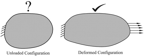
In this section, we present the inverse formulation to determine the unloaded configuration of a hyperelastic body. It is emphasized that by unloaded configuration we mean that the body is unloaded and free of initial/residual stresses. More precisely, we will solve for the boundary coordinates of the unloaded problem domain, while the material properties, the geometry of the boundary in the deformed configuration, and boundary conditions are given (see Figure ). The unknown boundary coordinates of the unloaded configuration are defined in vector representation as follows:
(12)
(12)
where
,
and
are components of the position vector of the jth node on the boundary of the body in three-dimensional space.
Figure 1. The hyperelastic body in its unloaded and deformed configurations.
The known or measured position vectors at boundary nodes are denoted by
(13)
(13)
where
,
and
are components of the position vector of the jth node on the boundary of the deformed body.
In the presented inverse method, manual mesh generation is performed just once for the given deformed configuration. For this mesh generation, a mesh study can be performed to make sure that the quality of the mesh is in accordance with the standards of the FEM. After discretizing the deformed body by a sufficient number of finite elements, the load in its reverse direction is applied to the deformed body to obtain an initial guess of the unloaded configuration (pre-calculated unloaded configuration). In this analysis, the deformed body is assumed to be stress-free because we have no information about the actual stress distribution in the deformed body and therefore, the pre-calculated unloaded configuration is just an estimation of the real one. The deformed mesh obtained by applying the reverse load can be used for the next analysis (the mesh for the initial guess). The quality of this mesh can also be studied and if it does not satisfy the standards of the FEM, the mesh can be manually modified. In succeeding steps of the optimization procedure, changes in the estimates of the unloaded configuration between two consecutive steps are small. Therefore, the mapping procedure can be utilized to generate the mesh for the domain in the next step. As a result, the quality of the mesh is preserved and no other controls are needed. The load in its actual direction is then applied to the pre-calculated unloaded configuration (initial guess in the first step of the inverse analysis) to obtain the position of the material points in the deformed configuration. The computed position vector for boundary nodes are represented with the following notation:
(14)
(14)
where
,
and
are the components of the position vector at the jth point on the boundary of the body. Next, we define a cost function as the difference between measured and computed boundary position vectors as follows:
(15)
(15)
We minimize Equation (15) for the unknown position vector of boundary nodes in the unloaded configuration. Different optimization techniques such as the Levenberg-Marquardt or Gauss–Newton methods can be employed to minimize the objective function in Equation (15). In the Gauss–Newton method, the calculated search direction may be too large and the inverse algorithm may not converge for some cases [Citation25]. Therefore, by adding a step factor to the conventional Gauss–Newton method, the damped Gauss–Newton method [Citation26,Citation27] is obtained in which by controlling the value of the step factor, the objective function in the step is forced to be smaller than the objective function in the Kth step [Citation26]. The damped Gauss–Newton method is employed in this study to minimize the objective function. This method is very efficient for solving inverse problems; see for example [Citation28,Citation29]. Hereby, the vector of unknowns is updated at each minimization step as follows:
(16)
(16)
where
is the step factor,
is the search direction and
is the step number. According to [Citation27], the first choice for the step factor
is one. If this value increases the objective function, the step factor is divided by two and the step is replicated. This procedure is repeated until the value of the cost function in the current step becomes less than its value in the previous step.
The search direction in Equation (16) is calculated as follows:
(17)
(17)
where
is the sensitivity matrix. The components of the sensitivity matrix are computed as follows:
(18)
(18)
Various techniques based on direct differentiation and finite difference approximation can be employed to calculate the components of the sensitivity matrix. In this study, the components of the vectors and
are the deformed
and undeformed
position vectors of the boundary nodes, respectively. The sensitivity coefficients in Equation (18) for each node is equal to the components of the deformation gradient
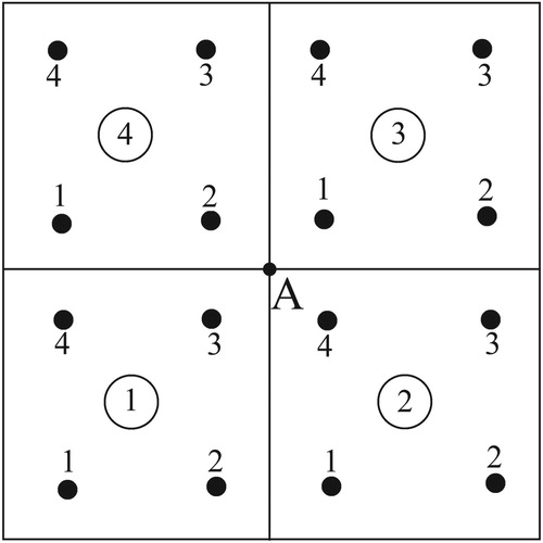
at that node. The deformation gradient is calculated at the element level. In the process of the problem solution, in order to compute element integrals, the components of the deformation gradient tensor are calculated at integration points. The deformation gradient tensor at nodes of the FE mesh is computed by an interpolation method using the values at the integration points. Therefore, during the solution of the direct problem in each step, the deformation gradient for boundary points obtained at the element level are stored to form the sensitivity matrix. For more clarification, suppose that we want to calculate the deformation gradient at the FE node A shown in Figure . This node belongs to four elements. During solution of the direct problem, the deformation gradients for all of the integration points within these four elements are stored. Therefore, by interpolating the deformation gradient tensor between 3rd integration point of element one, 4th integration point of element 2, 1st integration point of element 3 and 2nd integration point of element 4, the deformation gradient at node A is obtained. The algorithms of the present paper have been implemented in an in-house written MATLAB code.
Figure 2. Interpolating the deformation gradient tensor at a node of the FE mesh.
The optimization process for determination of the unknown unloaded configuration is repeated until a specified tolerance, , e.g. 0.1 percent of the largest measured displacement, is achieved for successive solutions of the position vectors according to
(19)
(19)
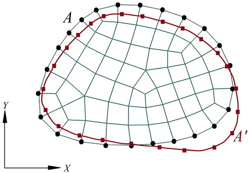
At each minimization step, a new estimate of the boundary node locations for the unloaded configuration is obtained and consequently, generation of interior mesh is required. For this purpose, the mesh used in the previous step is mapped for the newly calculated unloaded configuration. To this end, the Akin’s mapping method [Citation30,Citation31] will be used, which is based on the solution of the Laplace equation. In the following, we will briefly review this method. Let us define two consecutive unloaded configurations shown in Figure . Domain
is obtained in the kth step and we wish to generate a similar mesh for domain
in the
step. Now, suppose that each node with coordinates
,
and
in domain
is mapped into a node with coordinates
,
and
in domain
with
,
and
. Here,
,
and
are known everywhere on the boundary of domain
. To determine
,
and
for interior nodes in domain
, we solve Laplace’s equations given by:
(20)
(20)
(21)
(21)
(22)
(22)
Figure 3. Two consecutive calculated unloaded configurations.
Equations (20)–(22) are solved using the standard FEM [Citation32]. Finally, we can use ,
and
to update the mesh in domain
. We emphasize that the solution to Laplace’s equation only serves the purpose to update the mesh at each iteration and it is not for updating the deformation of the body. In the procedure of the optimization problem, updating the deformation of the body is neither performed by solving the Laplace equation nor by solving the linear elasticity problem. But, in each step of the optimization process, after performing the sensitivity analysis, the deformation of the body is updated by solving a hyperelastic problem. The algorithms of the presented method can be described as follows:
Step 1: Mesh the given deformed configuration of the body.
Step 2: Obtain the initial guess (pre-calculated unloaded configuration) by applying the load to the body in its reverse direction.
Step 3: Apply the load in its actual direction to the pre-calculated unloaded configuration.
Step 4: Compute the sensitivity matrix and update the position of the boundary nodes using the damped Gauss–Newton method.
Step 5: Re-mesh the domain of the current estimate for the unloaded configuration.
Step 6: Check to see if the specified tolerance is acquired. If not go to step 3.
4. Results and discussions
In this section, we present numerical examples in 2D and 3D as well as experimental examples to verify and validate the proposed method. All of the examples in this paper involve solely gravity loading, and we do not include external loading conditions that are applied actively. The main reason for this is that in many cases, actively applied loading conditions can be removed to obtain the unloaded configuration, while the same does not hold for gravity loading. Furthermore, we will investigate the effects of measurement and modelling errors on identifying the computed unloaded configuration. For the experimental part to validate this method, we chose a sample made of silicone material that is deformed under its own weight. We note that whenever displacement boundary conditions are imposed (here mainly fixed boundary conditions), the undeformed coordinates at these nodes are known, and thus, are not introduced as unknowns.
4.1. Numerical study in 2D
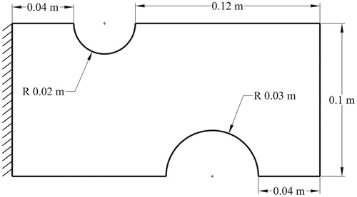
A hyperelastic solid with dimensions and boundary conditions as depicted in Figure in its unloaded configuration is considered. The left edge of the body is fixed and the body is deformed under its own weight with . A neo-Hookean material with model parameters
and
has been chosen to represent the mechanical behaviour of the body.
Figure 4. Dimensions of the hyperelastic body with fixed boundary conditions in its unloaded configuration.
No experiments are performed for this example, and we solely focus on the verification of the proposed method with synthetic data. In this case, the result of the inverse problem (undeformed configuration of the body) is exactly known. To this end, we create synthetic data by solving a boundary value problem. From the solution of this direct problem, we extract the deformed boundary and use it as the ‘measured’ data in the inverse problem.
The mesh consists of 220 four-node quadrilateral elements and 55 nodes are defined on the boundary. Therefore, the vector of unknown boundary positions in the unloaded configuration is given by:
(23)
(23)
where
and
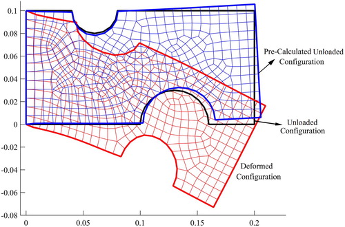
are components of the position vector of the jth node on the boundary of the body. Gravity is then applied in reverse direction to the deformed configuration to obtain a pre-calculated configuration, i.e. initial guess for the inverse analysis. The unloaded (exact), deformed, and pre-calculated configurations for plane stress and plane strain conditions are depicted in Figures and , respectively.
Figure 5. The unloaded, deformed and pre-calculated configurations of the body in the plane stress condition.
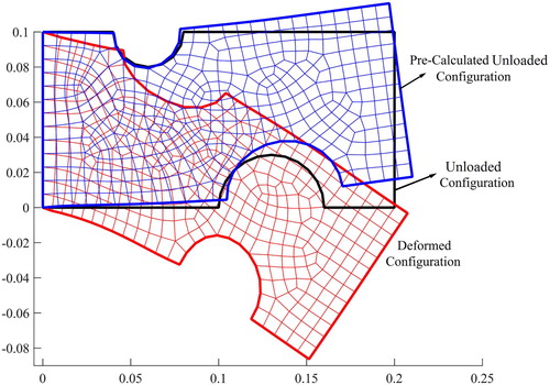
Figure 6. The unloaded, deformed and pre-calculated configurations of the body in plane strain condition.
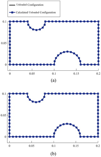
The recovered unloaded configurations in comparison with the exact ones for plane stress and plane strain conditions are depicted in Figure . For both plane stress and plane strain conditions, the inverse problem recovers the unloaded configuration very accurately.
Figure 7. The recovered unloaded configuration in comparison with the exact one in (a) the plane stress condition, (b) the plane strain condition.
Knowing the exact solution of the inverse problem in this example, we can define an error term as the difference between exact and calculated unloaded configurations as follows:
(24)
(24)
where
are the components of the position vector for boundary node
of the exact unloaded configuration. The error calculations for both, plane stress and plane strain conditions are provided in Table .
Table 1. The inverse problem results for plane stress and plane strain conditions.
It is observed that the computational cost for (1) the direct solver, (2) the sensitivity analysis and inverse solver, and (3) Laplace equation solver are 93.8%, 4%, and 2.2%, respectively. It should be mentioned that most of the matrices which are used in the sensitivity analysis are the same as those in the direct solver and they are not computed again.
Next, we compare the efficiency of the proposed method with the Sellier’s method [Citation19], which is a zero-order approach. Thus, we also solve the above inverse problem for plane strain with the Sellier’s method. The Sellier’s method starts with the given deformed configuration as the initial guess for the unknown unloaded configuration. In each step of the inverse analysis, the load in its actual direction is applied to the current estimate of the unloaded configuration, resulting in an approximate deformed configuration. The difference between the calculated deformed configuration and the actual one is computed and is subtracted from the approximate unloaded configuration to update it. The procedure is continued until convergence is achieved.
The results of the inverse problem for this case are also provided in Table and reveal that the proposed inverse algorithm recovers the unloaded configuration more efficiently using a gradient-based minimization approach. The computational cost of the proposed method was 6.2 times less than the Sellier’s method. It is noted that since Sellier’s method is based on a zero-order optimization method, it does not need sensitivity analysis and can be used with any direct solver code.
It is also noted that in all of the presented examples, a load, which produces a significant deformation, is considered. If a problem with a smaller deformation is considered, the problem approaches a linear problem, for which the required number of iterations by the zero-order method (Sellier’s method) approaches that of the first-order method (proposed method). On the other hand, for problems with large deformations, the nonlinearity of the problem increases and the number of iterations of Sellier’s method increases more than that of the proposed method.
Next, we ask the question of how the computational time would be affected if our method includes the coordinates of interior nodes in addition to the boundary nodes as unknowns. Thus, we solve the same inverse problem for the plane strain case with all the nodes in the FE mesh as unknowns instead of using only boundary nodes. The number of iterations and the solution error for this case are 7 and 0.028%, respectively. Our approach to optimize only for boundary nodes turns out to be 3.5 faster than optimizing for all nodes, which shows the efficiency of the proposed method.
In actual experiments, error in measurements is unavoidable. Additionally, the model used for describing the material response may not precisely represent the actual material behaviour. We will add these error sources by varying the model parameter of the neo-Hookean hyperelastic model. Changing
from 2400 to 2300 Pa leads to a maximum error of 3% in the displacement field in the deformed configuration. The results for the plane strain condition are provided in Table . It should be noted that the exact solution corresponds to
, while the inverse problem has been solved with
.
Table 2. Results of the inverse problem for the plane strain case with different levels of added errors in the input data.
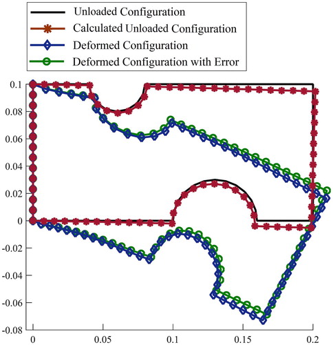
Next, we assume that the actual model parameter is , while we solve the inverse problem with an assumed model parameter
. This creates a maximum error of 6% in the displacement field. In Table , the results of the inverse problem for this case are summarized.
The unloaded configuration (exact), computed unloaded configuration, deformed configuration of the body with 6% error and without measurement error are depicted in Figure . From this figure it can be seen that when the amount of error in the displacements of deformed configuration is increased, the unloaded configuration is recovered with less accuracy; however, the result appears to be reasonable with a solution error of 2.34%.
Figure 8. The unloaded configuration and calculated unloaded configuration together with deformed configurations of the body with 6% error and without error in the input data for the plane strain condition.
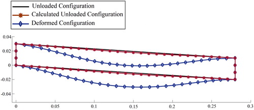
4.2. Validation with experimental data
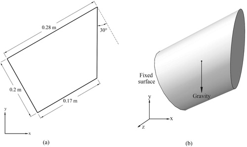
In this section, we will collect measurements from actual experiments and solve the inverse problem. A sample made of silicone with dimensions shown in Figure was fabricated. The neo-Hookean model parameters for the silicone sample were known with and
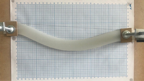
. Since the thickness of the specimen was relatively small (8 mm), the problem has been solved under the plane stress condition. Further, we fixed the silicone sample at two edges as shown in Figure and placed it on a graph paper with resolution of 1 mm. At first, the specimen was placed in horizontal position and leaning on the plate underneath, such that gravity did not deform it much. This state was considered to be the unloaded configuration of the body. The specimen is then placed vertically to allow gravity to bend it under its own weight as shown in Figure . The position of the boundary nodes in this configuration are the measured data for the inverse problem.
Figure 9. Dimensions of the silicone body.
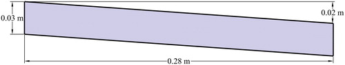
Figure 10. The silicone body in the horizontal state.
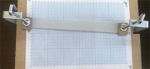
Figure 11. The silicone body in the vertical position.
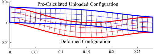
The deformed configuration of the specimen with a manually generated mesh and the pre-calculated configuration with the mapped mesh are depicted in Figure .
Figure 12. The deformed and pre-calculated configurations of the silicone body.
After 7 iterations, the unloaded configuration of the silicone sample was recovered as shown in Figure . We observe that the presented method has calculated the unloaded configuration of the silicone body with good accuracy.
Figure 13. The unloaded, deformed, and calculated unloaded configurations of the silicone body.
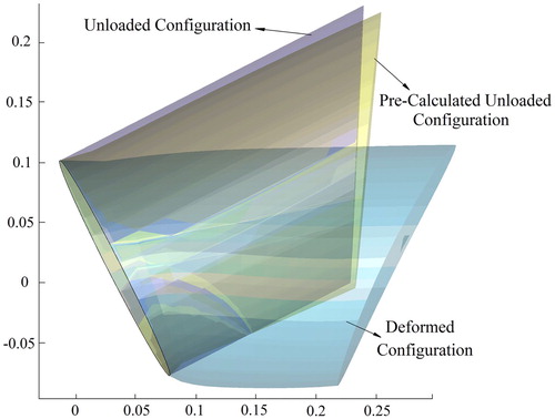
4.3. Numerical study in 3D
In this section, we test the proposed method with a hyperelastic material in 3D, having a relatively complicated geometry as depicted in Figure in its unloaded configuration. The posterior surface of the body is fixed and the body is deformed under its own weight with . The Mooney-Rivlin hyperelastic material model with constants
,
and
is employed to simulate the mechanical behaviour of the body. First, the direct problem is solved and the positions of boundary (here a surface) nodes in the deformed configuration are extracted and utilized as measured data for the inverse problem.
Figure 14. Dimensions and boundary conditions of the 3D hyperelastic body in its unloaded configuration, (a) side view, (b) 3D view.
A mesh of 1419 eight-node brick elements is generated within the domain of the deformed body. This mesh has 487 nodes on the surface (boundary) of the body. Therefore, the vector of unknowns is given by:
(25)
(25)
where
,
and
are components of the position vector of the jth node on the surface of the body. Gravitational load is then applied in reverse direction to the deformed configuration of the body to obtain an initial guess for the inverse analysis. The unloaded, deformed and pre-calculated configurations of the body are depicted in Figure .
Figure 15. The unloaded, deformed and pre-calculated configurations of the body.
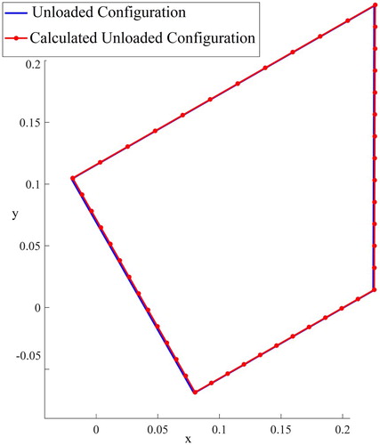
The inverse problem recovers the unloaded configuration of the body after 7 iterations very accurately. The recovered unloaded configuration in the x-y plane in comparison to the exact one is depicted in Figure .
Figure 16. The recovered unloaded configuration in x-y plane in comparison to the exact unloaded configuration.
5. Conclusions
In this paper, a gradient-based inverse method was presented that employed boundary-only variables to identify the unloaded configuration of a hyperelastic body. The Akin’s mesh mapping method was used to avoid manual mesh generation in each step of the inverse analysis. We verified the effectiveness of the method with 2D problems under plane stress and plane strain conditions in a numerical study. It was observed that the proposed gradient-based algorithm performs significantly better than the existing zero-order method. The effect of errors on identification of the unloaded configuration was also investigated. It was observed that when the error in measured data and material model increased, the unloaded configuration was obtained with less accuracy; however, it was still acceptable. To validate this approach, a silicone-based specimen was created and the proposed inverse method was employed to retrieve its unloaded configuration after being deformed under its weight. Despite the presence of inherent error in the experimental example, the unloaded configuration was recovered accurately. The efficiency of the proposed algorithm was also examined with a 3D numerical example having a relatively complicated geometry.
We note that, in this work the type of loading on the body was gravity. However, the presented method can be employed to identify the unloaded configuration of the body with any other type of loading as well. We also emphasize that the neo-Hookean and Mooney-Rivlin hyperelastic models were employed to describe mechanical behaviour of the body in this study, but, the presented inverse method can be used with other hyperelastic models as well.
Disclosure statement
No potential conflict of interest was reported by the authors.
ORCID
M. R. Hematiyan http://orcid.org/0000-0001-8926-7163
References
- Govindjee S, Mihalic PA. Computational methods for inverse finite elastostatics. Comput Methods Appl Mech Eng. 1996;136(1-2):47–57. doi: 10.1016/0045-7825(96)01045-6
- Govindjee S, Mihalic PA. Computational methods for inverse deformations in quasi-incompressible finite elasticity. Int J Numer Methods Eng. 1998;43(5):821–838. doi: 10.1002/(SICI)1097-0207(19981115)43:5<821::AID-NME453>3.0.CO;2-C
- Lapuebla-Ferri A, del Palomar AP, Herrero J, et al. A patient-specific FE-based methodology to simulate prosthesis insertion during an augmentation mammoplasty. Med Eng Phys. 2011;33(9):1094–1102. doi: 10.1016/j.medengphy.2011.04.014
- Rajagopal V, Lee A, Chung JH, et al. Creating individual-specific biomechanical models of the breast for medical image analysis. Acad Radiol. 2008;15(11):1425–1436. doi: 10.1016/j.acra.2008.07.017
- Lee AW, Rajagopal V, Gamage TPB, et al. Breast lesion co-localisation between X-ray and MR images using finite element modelling. Med Image Anal. 2013;17(8):1256–1264. doi: 10.1016/j.media.2013.05.011
- Lorensen WE, Cline HE. Marching cubes: A high resolution 3D surface construction algorithm. In ACM Siggraph Computer Graphics. 1987;21(4):163–169. doi: 10.1145/37402.37422
- Rajagopal V, Chung JH, Bullivant D, et al. Determining the finite elasticity reference state from a loaded configuration. Int J Numer Methods Eng. 2007;72(12):1434–1451. doi: 10.1002/nme.2045
- Rajagopal V, Nash MP, Highnam RP, et al. (2008). The breast biomechanics reference state for multi-modal image analysis. Paper presented at: International Workshop on Digital Mammography.
- Pathmanathan P, Gavaghan D, Whiteley J, et al. (2004). Predicting tumour location by simulating large deformations of the breast using a 3D finite element model and nonlinear elasticity. Paper presented at: International Conference on Medical Image Computing and Computer-Assisted Intervention.
- Carter T, Tanner C, Beechey-Newman N, et al. (2008). MR navigated breast surgery: method and initial clinical experience. Paper presented at: International Conference on Medical Image Computing and Computer-Assisted Intervention.
- Eiben B, Han L, Hipwell J, et al. (2013). Biomechanically guided prone-to-supine image registration of breast MRI using an estimated reference state. Paper presented at: Biomedical Imaging (ISBI), 2013 IEEE 10th International Symposium on.
- Eiben B, Vavourakis V, Hipwell JH, et al. (2014). Breast deformation modelling: comparison of methods to obtain a patient specific unloaded configuration. Paper presented at: Medical Imaging 2014: Image-Guided Procedures, Robotic Interventions, and Modeling.
- Eder M, Raith S, Jalali J, et al. Comparison of different material models to simulate 3-d breast deformations using finite element analysis. Ann Biomed Eng. 2014;42(4):843–857. doi: 10.1007/s10439-013-0962-8
- Raghavan M, Ma B, Fillinger MF. Non-invasive determination of zero-pressure geometry of arterial aneurysms. Ann Biomed Eng. 2006;34(9):1414–1419. doi: 10.1007/s10439-006-9115-7
- Bols J, Degroote J, Trachet B, et al. A computational method to assess the in vivo stresses and unloaded configuration of patient-specific blood vessels. J Comput Appl Math. 2013;246:10–17. doi: 10.1016/j.cam.2012.10.034
- Riveros F, Chandra S, Finol EA, et al. A pull-back algorithm to determine the unloaded vascular geometry in anisotropic hyperelastic AAA passive mechanics. Ann Biomed Eng. 2013;41(4):694–708. doi: 10.1007/s10439-012-0712-3
- Vavourakis V, Hipwell JH, Hawkes DJ. An inverse finite element u/p-formulation to predict the unloaded state of in vivo biological soft tissues. Ann Biomed Eng. 2016;44(1):187–201. doi: 10.1007/s10439-015-1405-5
- Nikou A, Dorsey SM, McGarvey JR, et al. Effects of using the unloaded configuration in predicting the in vivo diastolic properties of the heart. Comput Methods Biomech Biomed Engin. 2016;19(16):1714–1720. doi: 10.1080/10255842.2016.1183122
- Sellier M. An iterative method for the inverse elasto-static problem. J Fluids Struct. 2011;27(8):1461–1470. doi: 10.1016/j.jfluidstructs.2011.08.002
- Rausch MK, Genet M, Humphrey JD. An augmented iterative method for identifying a stress-free reference configuration in image-based biomechanical modelling. J Biomech. 2017;58:227–231. doi: 10.1016/j.jbiomech.2017.04.021
- Malvern LE. (1969). Introduction to the mechanics of a continuous medium (No. Monograph).
- Bower AF. Applied mechanics of solids. Boca Raton, FL: CRC press; 2009.
- Hajhashemkhani M, Hematiyan MR, Goenezen S. Identification of material parameters of a hyper-elastic body with unknown boundary conditions. J Appl Mech. 2018;85(5):051006. doi: 10.1115/1.4039170
- Lai WM, Rubin DH, Krempl E, et al. Introduction to continuum mechanics. Oxford: Butterworth-Heinemann; 2009.
- Taylor DG, Li S. (2003, November). Damped Gauss-Newton method for direct stable inversion of continuous-time nonlinear systems. In IECON'03: 29th Annual Conference of the IEEE Industrial Electronics Society (IEEE Cat. No. 03CH37468) (Vol. 1, pp. 606–610). IEEE.
- Ortega JM, Rheinboldt WC. (1970). Iterative solution of nonlinear equations in several variables (Vol. 30): SIAM.
- Bjorck A. (1996). Numerical methods for least squares problems (Vol. 51): SIAM.
- Hematiyan MR, Khosravifard A, Shiah YC. A new stable inverse method for identification of the elastic constants of a three-dimensional generally anisotropic solid. Int J Solids Struct. 2017;106:240–250. doi: 10.1016/j.ijsolstr.2016.11.009
- Hajhashemkhani M, Hematiyan MR, Goenezen S. Inverse determination of elastic constants of a hyper-elastic member with inclusions using simple displacement/length measurements. The Journal of Strain Analysis for Engineering Design. 2018;53(7):529–542. doi: 10.1177/0309324718792452
- Akin J. Application and implementation of finite element methods. London: Academic Press, Inc; 1982.
- Hannaby S. A mapping method for mesh generation. Comput Math Appl. 1988;16(9):727–735. doi: 10.1016/0898-1221(88)90008-9
- Reddy JN. An Introduction to nonlinear finite element analysis: with applications to heat transfer, fluid mechanics, and solid mechanics. Oxford: OUP; 2014.