Improving a Tikhonov regularization method with a fractional-order differential operator for the inverse black body radiation problem

Abstract

Tikhonov regularization is an usual method to solve an ill-posed problem, recommended when the input data are contaminated with noise. However, in some cases, the use of this technique is not sufficient to provide good solutions. In this work, an improvement of the Tikhonov regularization method was proposed and tested in the inverse black body radiation problem. The method proposed consisted in including the norm of the fractional-order derivative of the solution in the original functional proposed by Tikhonov. In the present framework, the regularized solution depends on the regularization parameter, λ, and on the fractional derivative order, α. For α assuming real value between 0 and 2, the solution obtained is more precise than those from the usual Tikhonov regularization method.

Keywords:

• Fractional calculus
• ill-posed problem
• Grünwald–Letnikov derivative
• Tikhonov regularization method

2010 Mathematics Subject Classifications:

• 26A33
• 35R30

1. Introduction

Inverse problems in physical-chemistry research area deal with retrieving information from experimental data. Without noise on experimental data, the solution can be exactly recovered. However, with a minimum error on input data, which is the common case in physical-chemistry research, the solution is not stable or unique [1]. In this case, there are many results that minimize the Euclidian norm of the residual vector, but a lot of them do not satisfy the physical requirements of the problem, such as a finite norm of the solution.

To circumvent this difficulty, ordinarily the Tikhonov regularization method is used, method developed independently by Phillips [2] and Tikhonov [3]. This method proposes a new criterion for evaluating adequate physical solution, which includes Euclidean norm of the first-order derivative of the solution, beyond usual Euclidian norm of the residual vector. The regularization parameter represents the weight given to the additional restriction in usual residual norm criterion. The Tikhonov method has been used for many applications with great success, as shown in Refs. [4–7]. However, in some cases, the solution obtained by the Tikhonov method converges to solutions which are oscillating and do not provide physically adequate results of the problem, although the solution found minimizes a norm of the residual vector. In this case, new procedures are needed.

The purpose of this study is to describe and to examine an improved Tikhonov regularization method, which includes Euclidean norm of the fractional-order derivative of the solution as an additional criterion. In this paper, Grünwald–Letnikov (GL) fractional derivative will be used to generalize the derivative concept from integer order to non-integer order [8, 9]. Of the many definitions for fractional order derivative, the GL definition is the most often used, being equivalent to a Riemann–Liouville derivative [8]. Recently, many papers in the literature have reported the use of fractional-order derivative as a better alternative than integer-order derivative [10–12]. However, the improvement proposed here has not yet been explored in the literature.

The inverse black body radiation will be used as prototype to explore and analyse the method proposed in this paper [13]. The problem consists in determining the surface temperature distribution of a black body source from the radiated power spectrum. The problem is of great interest in remote sensing and astrophysics [14, 15]. As we shall see, most solutions presented in the literature are unstable when experimental errors are taken into account.

Bojarski proposed, in 1982, the first solution for this problem in terms of iterative procedure and inverse Laplace transform for the radiated power spectrum [13]. Following Bojarski's work, various papers provided different improvements on his solution [16, 17]. All these papers involved the use of the inverse Laplace transform and in all of the works mentioned above, only very few simple numerical examples were presented, in general without including experimental uncertainties.

In 1990, Nanxian presented one solution that used modified Möbius inverse formula; this method showed more favourable results when compared with previous algorithms [18]. Afterwards, Nanxian and Guangyin proposed a method based on Fourier transform with quite good results [17]. All the previous methods are generally quite sensitive to noise in the input data. Therefore, the difficulty to determine stable solution when experimental data are involved still remains.

The difficulty of finding a stable solution is due to the ill-posed character of the problem. Tikhonov regularization is the most commonly used method to find stable solution for ill-posed problems [2, 3]. The use of Tikhonov regularization technique in the inverse black body radiation problem was made for the first time by Xiaoguang in 1987. In this last work, triangular area temperature distribution and low temperature were used as prototype for testing [19].

Subsequently, various authors provided different improvements to solve this problem by using different regularization techniques [20, 21]. The Tikhonov method has been a very powerful tool in filtering out the influence of noise. However, as we shall see, more efficient methods are needed in order to minimize oscillations in the solution.

In the present study, for the first time, we employ the norm of the fractional derivative order as restriction in functional proposed by Tikhonov in your regularization method. In this work, we will show that the proposed method provides a stable solution, which is the best when compared with usual technique.

In Section 2, we will begin by introducing our generalized model and the necessary foundations of fractional calculus are presented. The prototype problem for the examination of the method proposed is presented in Section 3 together with discussion of the efficiency of the strategy proposed here. Then, in Section 4, the conclusions are summarized.

2. Methodology

2.1. Generalized Tikhonov functional

The interpretation of results of an experimental measurement requires a physical-chemistry model, which can be expressed as $\mathbf{K}\mathbf{f}=\mathbf{g}$. The inverse problem consists in determination of $\mathbf{f}$ by knowing the $\mathbf{g}$ and the $\mathbf{K}$, in which $\mathbf{g}$ is direct experimental measurement and $\mathbf{f}$ is indirect information obtained from $\mathbf{g}$.

The difficulties in solving inverse problems are caused by experimental error in input data. In this case, the usual solution procedure is unstable, which leads to large errors in the final results. Due to this fact, the problem is called ill-posed [2]. The Tikhonov method was proposed by Tikhonov in 1963 [3] and it is the most commonly used strategy to solve ill-posed problems, with success in many cases [2, 3, 22, 23]. The Tikhonov method consists in finding the solution which makes minimum the function ${\varphi }_{\lambda }(\mathbf{f})$, where ${\varphi }_{\lambda }(\mathbf{f})$ is given by Phillips [2] (1) ${\varphi }_{\lambda }(\mathbf{f})=\Vert \mathbf{K}(\mathbf{f})-\mathbf{g}{\Vert }^2+{\lambda }^2(a_0\Vert \mathbf{f}{\Vert }^2+a_1\Vert {\mathbf{f}}^{\mathrm{\prime }}{\Vert }^2+a_2\Vert {\mathbf{f}}^{\mathrm{\prime }\mathrm{\prime }}{\Vert }^2).$(1) In Equation (1(1) ${\varphi }_{\lambda }(\mathbf{f})=\Vert \mathbf{K}(\mathbf{f})-\mathbf{g}{\Vert }^2+{\lambda }^2(a_0\Vert \mathbf{f}{\Vert }^2+a_1\Vert {\mathbf{f}}^{\mathrm{\prime }}{\Vert }^2+a_2\Vert {\mathbf{f}}^{\mathrm{\prime }\mathrm{\prime }}{\Vert }^2).$(1) ), the prime symbol is the first-order derivative of $\mathbf{f}$ and the double prime symbol is used to represent the second-order derivative of $\mathbf{f}$. Parameters $a_0$, $a_1$ and $a_2$ are keys, which are used to lock ($a_i=1$) and unlock ($a_i=0$) the additional restriction on square residual norm. The regularization parameter λ represents the weight given to the additional restriction. This additional restriction can provide a stable approximate solution, Equation (2(2) $\begin{array}{rl}{\mathbf{f}}_{\lambda }& =\underset{\mathbf{f}}{min}{\varphi }_{\lambda }(\mathbf{f}),\\ {\mathbf{f}}_{\lambda }& =\{{\mathbf{K}}^T\mathbf{K}+{\lambda }^2(a_0{\mathbf{D}}^{(0)}+a_1{\mathbf{D}}^{(1)}+a_2{\mathbf{D}}^{(2)}){\}}^{-1}{\mathbf{K}}^T\mathbf{g}.\end{array}$(2) ), which depends on the regularization parameter chosen. (2) $\begin{array}{rl}{\mathbf{f}}_{\lambda }& =\underset{\mathbf{f}}{min}{\varphi }_{\lambda }(\mathbf{f}),\\ {\mathbf{f}}_{\lambda }& =\{{\mathbf{K}}^T\mathbf{K}+{\lambda }^2(a_0{\mathbf{D}}^{(0)}+a_1{\mathbf{D}}^{(1)}+a_2{\mathbf{D}}^{(2)}){\}}^{-1}{\mathbf{K}}^T\mathbf{g}.\end{array}$(2) In Equation (2(2) $\begin{array}{rl}{\mathbf{f}}_{\lambda }& =\underset{\mathbf{f}}{min}{\varphi }_{\lambda }(\mathbf{f}),\\ {\mathbf{f}}_{\lambda }& =\{{\mathbf{K}}^T\mathbf{K}+{\lambda }^2(a_0{\mathbf{D}}^{(0)}+a_1{\mathbf{D}}^{(1)}+a_2{\mathbf{D}}^{(2)}){\}}^{-1}{\mathbf{K}}^T\mathbf{g}.\end{array}$(2) ), ${\mathbf{D}}^{(0)}$ is the identity matrix $\mathbf{I}$, ${\mathbf{D}}^{(1)}$ is the matrix form of the first-order derivative operator and ${\mathbf{D}}^{(2)}$ is the matrix representation of the second-order derivative operator [24] (3) $\begin{array}{rl}{\mathbf{D}}^{(0)}& =\mathbf{I},\end{array}$(3) (4) $\begin{array}{rl}{\mathbf{D}}^{(1)}& =\left[\begin{array}{ccccc}1& -1& & & \\ -1& 2& -1& & \\ & \ddots & \ddots & \ddots & \\ & & -1& 2& -1\\ & & & -1& 1\end{array}\right]\end{array}$(4) and (5) ${\mathbf{D}}^{(2)}=\left[\begin{array}{ccccccc}1& -2& 1& & & & \\ -2& 5& -4& 1& & & \\ 1& -4& 6& -4& 1& & \\ & \ddots & \ddots & \ddots & \ddots & \ddots & \\ & & 1& -4& 6& -4& 1\\ & & & 1& -4& 5& -2\\ & & & & 1& -2& 1\end{array}\right].$(5)

When λ is equal to zero, the solution found minimizes the residual, but in general with large norm for the solution. On the other hand, if λ is large we find a solution with finite norm, but the norm of the residual is quite large. There is one λ that establishes the good balance between the norm of the solution and the residual norm, providing an acceptable solution. The optimal regularization parameter is chosen usually by L-curve; however, this method may fail to determine the appropriate regularization parameter. In this paper, the L-curve was used to get the initial regularization parameter, which was later refined by comparison between exact and recovered solution [25].

This strategy can be improved by using non-integer derivative operator, then (6) ${\varphi }_{\lambda ,\alpha }(\mathbf{f})=\Vert \mathbf{K}(\mathbf{f})-\mathbf{g}{\Vert }^2+{\lambda }^2\Vert \frac{{\mathrm{d}}^{\alpha }\mathbf{f}}{\mathrm{d}{t}^{\alpha }}{\Vert }^2;$(6) therefore, the solution can be obtained by (7) $\begin{array}{rl}{\mathbf{f}}_{\lambda ,\alpha }& =\underset{\mathbf{f}}{min}{\varphi }_{\lambda ,\alpha }(\mathbf{f}),\\ {\mathbf{f}}_{\lambda ,\alpha }& =\{{\mathbf{K}}^T\mathbf{K}+{\lambda }^2{\mathbf{D}}^{(\alpha )}{\}}^{-1}{\mathbf{K}}^T\mathbf{g},\end{array}$(7) where ${\mathbf{D}}^{(\alpha )}$ is the GL operator for the fractional derivative and α is the derivative order. The result presented in Equation (7(7) $\begin{array}{rl}{\mathbf{f}}_{\lambda ,\alpha }& =\underset{\mathbf{f}}{min}{\varphi }_{\lambda ,\alpha }(\mathbf{f}),\\ {\mathbf{f}}_{\lambda ,\alpha }& =\{{\mathbf{K}}^T\mathbf{K}+{\lambda }^2{\mathbf{D}}^{(\alpha )}{\}}^{-1}{\mathbf{K}}^T\mathbf{g},\end{array}$(7) ) can be obtained by procedures similar to those for Equation (2(2) $\begin{array}{rl}{\mathbf{f}}_{\lambda }& =\underset{\mathbf{f}}{min}{\varphi }_{\lambda }(\mathbf{f}),\\ {\mathbf{f}}_{\lambda }& =\{{\mathbf{K}}^T\mathbf{K}+{\lambda }^2(a_0{\mathbf{D}}^{(0)}+a_1{\mathbf{D}}^{(1)}+a_2{\mathbf{D}}^{(2)}){\}}^{-1}{\mathbf{K}}^T\mathbf{g}.\end{array}$(2) ), which were presented in Ref. [24]. Now regularized solution depends on the regularization parameter, λ, and fractional derivative order, α. The GL fractional derivative operator has not been used before in the present context. The question about how α has an effect on solution $\mathbf{f}$, at λ fixed, will be discussed in Section 3.

When $\alpha =0$, the solution from Equation (7(7) $\begin{array}{rl}{\mathbf{f}}_{\lambda ,\alpha }& =\underset{\mathbf{f}}{min}{\varphi }_{\lambda ,\alpha }(\mathbf{f}),\\ {\mathbf{f}}_{\lambda ,\alpha }& =\{{\mathbf{K}}^T\mathbf{K}+{\lambda }^2{\mathbf{D}}^{(\alpha )}{\}}^{-1}{\mathbf{K}}^T\mathbf{g},\end{array}$(7) ) is equal to the case in which $a_0=1$, $a_1=0$ and $a_2=0$ in Equation (2(2) $\begin{array}{rl}{\mathbf{f}}_{\lambda }& =\underset{\mathbf{f}}{min}{\varphi }_{\lambda }(\mathbf{f}),\\ {\mathbf{f}}_{\lambda }& =\{{\mathbf{K}}^T\mathbf{K}+{\lambda }^2(a_0{\mathbf{D}}^{(0)}+a_1{\mathbf{D}}^{(1)}+a_2{\mathbf{D}}^{(2)}){\}}^{-1}{\mathbf{K}}^T\mathbf{g}.\end{array}$(2) ). For $a_0=0$, $a_1=1$ and $a_2=0$ in Equation (2(2) $\begin{array}{rl}{\mathbf{f}}_{\lambda }& =\underset{\mathbf{f}}{min}{\varphi }_{\lambda }(\mathbf{f}),\\ {\mathbf{f}}_{\lambda }& =\{{\mathbf{K}}^T\mathbf{K}+{\lambda }^2(a_0{\mathbf{D}}^{(0)}+a_1{\mathbf{D}}^{(1)}+a_2{\mathbf{D}}^{(2)}){\}}^{-1}{\mathbf{K}}^T\mathbf{g}.\end{array}$(2) ), it provides the same result that $\alpha =1$ in Equation (7(7) $\begin{array}{rl}{\mathbf{f}}_{\lambda ,\alpha }& =\underset{\mathbf{f}}{min}{\varphi }_{\lambda ,\alpha }(\mathbf{f}),\\ {\mathbf{f}}_{\lambda ,\alpha }& =\{{\mathbf{K}}^T\mathbf{K}+{\lambda }^2{\mathbf{D}}^{(\alpha )}{\}}^{-1}{\mathbf{K}}^T\mathbf{g},\end{array}$(7) ). Finally, Equations (2(2) $\begin{array}{rl}{\mathbf{f}}_{\lambda }& =\underset{\mathbf{f}}{min}{\varphi }_{\lambda }(\mathbf{f}),\\ {\mathbf{f}}_{\lambda }& =\{{\mathbf{K}}^T\mathbf{K}+{\lambda }^2(a_0{\mathbf{D}}^{(0)}+a_1{\mathbf{D}}^{(1)}+a_2{\mathbf{D}}^{(2)}){\}}^{-1}{\mathbf{K}}^T\mathbf{g}.\end{array}$(2) ) and  (7(7) $\begin{array}{rl}{\mathbf{f}}_{\lambda ,\alpha }& =\underset{\mathbf{f}}{min}{\varphi }_{\lambda ,\alpha }(\mathbf{f}),\\ {\mathbf{f}}_{\lambda ,\alpha }& =\{{\mathbf{K}}^T\mathbf{K}+{\lambda }^2{\mathbf{D}}^{(\alpha )}{\}}^{-1}{\mathbf{K}}^T\mathbf{g},\end{array}$(7) ) lead to the same result when $a_0=0$, $a_1=0$ and $a_2=1$, with $\alpha =2$ in derivative order. Out of these special cases, there are many solutions which are not contained in solution space of Equation (2(2) $\begin{array}{rl}{\mathbf{f}}_{\lambda }& =\underset{\mathbf{f}}{min}{\varphi }_{\lambda }(\mathbf{f}),\\ {\mathbf{f}}_{\lambda }& =\{{\mathbf{K}}^T\mathbf{K}+{\lambda }^2(a_0{\mathbf{D}}^{(0)}+a_1{\mathbf{D}}^{(1)}+a_2{\mathbf{D}}^{(2)}){\}}^{-1}{\mathbf{K}}^T\mathbf{g}.\end{array}$(2) ) but are contained in solution space of Equation (7(7) $\begin{array}{rl}{\mathbf{f}}_{\lambda ,\alpha }& =\underset{\mathbf{f}}{min}{\varphi }_{\lambda ,\alpha }(\mathbf{f}),\\ {\mathbf{f}}_{\lambda ,\alpha }& =\{{\mathbf{K}}^T\mathbf{K}+{\lambda }^2{\mathbf{D}}^{(\alpha )}{\}}^{-1}{\mathbf{K}}^T\mathbf{g},\end{array}$(7) ) in which $\alpha \in {\mathrm{\Re }}^{+}$ and $0\le \alpha \le 2$. Details of the GL derivative will be presented in Section 2.2.

2.2. Fractional calculus background

The GL definition of fractional derivatives is a generalization of the formula for the nth derivative of $f(t)$, with $n=1,2,3,\dots$ (8) $\frac{{\mathrm{d}}^{n}f(t)}{\mathrm{d}{t}^n}=\underset{h\to 0}{lim}\frac{1}{h^n}\sum _{k=0}^n(-1{)}^k{C}_{n,k}f(t-kh)$(8) with the binomial coefficient defined by $C_{n,k}=n!/k!(n-k)!$ For Equation (8(8) $\frac{{\mathrm{d}}^{n}f(t)}{\mathrm{d}{t}^n}=\underset{h\to 0}{lim}\frac{1}{h^n}\sum _{k=0}^n(-1{)}^k{C}_{n,k}f(t-kh)$(8) ) to be valid for n non-integer number, the binomial coefficients can be defined as (9) $C_{n,k}=\frac{\mathrm{\Gamma }(n+1)}{\mathrm{\Gamma }(k+1)\mathrm{\Gamma }(n-k+1)},$(9) whereas $\mathrm{\Gamma }(.)$ is the gamma function, an interpolation function for the factorial $n!$ when the argument n + 1 is a non-integer number.

Equation (8(8) $\frac{{\mathrm{d}}^{n}f(t)}{\mathrm{d}{t}^n}=\underset{h\to 0}{lim}\frac{1}{h^n}\sum _{k=0}^n(-1{)}^k{C}_{n,k}f(t-kh)$(8) ) can be rewritten as [8] (10) ${[}^{GL}{D}_0^{(\alpha )}f](t)=\underset{h\to 0^{+}}{lim}\frac{1}{h^{\alpha }}\sum _{k=0}^N(-1{)}^k{C}_{\alpha ,k}f(t-kh)$(10) with α in place of n and $\alpha \in {\mathrm{\Re }}^{+}$. The total terms in the sum $N=\lceil t/h\rceil$ is the smallest integer such that $N>t/h$. The GL fractional derivative of f, ${[}^{GL}{D}_0^{(\alpha )}f](t)$, has also a matrix form representation as, $\mathbf{d}={\mathbf{D}}^{(\alpha )}\mathbf{f}$, with (11) $\begin{array}{rl}{\mathbf{D}}^{(\alpha )}& =\frac{1}{h^{\alpha }}[\begin{array}{ccc}{C}_{\alpha ,0}& 0& 0\\ -C_{\alpha ,1}& C_{\alpha ,0}& 0\\ C_{\alpha ,2}& -C_{\alpha ,1}& C_{\alpha ,0}\\ \cdots & \cdots & \cdots \\ (-1{)}^N{C}_{\alpha ,N}& (-1{)}^{N-1}{C}_{\alpha ,N-1}& (-1{)}^{N-2}{C}_{\alpha ,N-2}\end{array}\\ & \begin{array}{ccc}0& \cdots & 0\\ 0& \cdots & 0\\ 0& \cdots & 0\\ \cdots & \cdots & \cdots \\ (-1{)}^{N-3}{C}_{\alpha ,N-3}& \cdots & C_{\alpha ,0}\end{array}],\end{array}$(11) $\mathbf{f}=[f(0)f(h)f(2h)\dots f(Nh){]}^T$ and $\mathbf{d}=[{[}^{GL}{D}_0^{(\alpha )}f](0){[}^{GL}{D}_0^{(\alpha )}f](h)\cdots {[}^{GL}{D}_0^{(\alpha )}f](Nh)]$. A proof of this result can be found in Ref. [8]. Here, recursive formula was used to calculate binomial coefficients [8].

Some properties of GL fractional derivative are [8] (a) the GL fractional derivative of order zero returns the original function; (b) the GL fractional derivative of integer order n gives the same result as the usual differentiation of order n; (c) the GL fractional derivative is a non-local operator, as it is evident from the sum in Equation (10(10) ${[}^{GL}{D}_0^{(\alpha )}f](t)=\underset{h\to 0^{+}}{lim}\frac{1}{h^{\alpha }}\sum _{k=0}^N(-1{)}^k{C}_{\alpha ,k}f(t-kh)$(10) ) and (d) the GL fractional derivative is an ill-posed operator; this means that small errors in input data may yield large errors in the output result.

The non-local property of the fractional operators (item c) is presented in Equation (7(7) $\begin{array}{rl}{\mathbf{f}}_{\lambda ,\alpha }& =\underset{\mathbf{f}}{min}{\varphi }_{\lambda ,\alpha }(\mathbf{f}),\\ {\mathbf{f}}_{\lambda ,\alpha }& =\{{\mathbf{K}}^T\mathbf{K}+{\lambda }^2{\mathbf{D}}^{(\alpha )}{\}}^{-1}{\mathbf{K}}^T\mathbf{g},\end{array}$(7) ), which does not appear in Equation (2(2) $\begin{array}{rl}{\mathbf{f}}_{\lambda }& =\underset{\mathbf{f}}{min}{\varphi }_{\lambda }(\mathbf{f}),\\ {\mathbf{f}}_{\lambda }& =\{{\mathbf{K}}^T\mathbf{K}+{\lambda }^2(a_0{\mathbf{D}}^{(0)}+a_1{\mathbf{D}}^{(1)}+a_2{\mathbf{D}}^{(2)}){\}}^{-1}{\mathbf{K}}^T\mathbf{g}.\end{array}$(2) ). This fact provided the motivation for a change in the Tikhonov method based on derivative with non-integer order.

3. Results and discussions

This paper proposes to explore the effect of inclusion of a fractional order operator on the Tikhonov method. One example is chosen to provide a test of the method proposed here.

3.1. Inverse black body radiation problem

The example chosen deals with the inverse black body radiation problem. It is well-known that a black body at temperature T emits a spectrum which is given by Planck's law. However, if parts of body's surface are not at the same temperature, the total power spectrum radiated is given by Equation (12(12) $g(\nu )=\frac{2h{\nu }^3}{c^2}{\int }_0^{\mathrm{\infty }}\frac{1}{e^{h\nu /kT}-1}f(T)\mathrm{d}T\approx {\int }_0^{T_{max}}K(\nu ,T)f(T)\mathrm{d}T.$(12) ). The problem defined by Equation (12(12) $g(\nu )=\frac{2h{\nu }^3}{c^2}{\int }_0^{\mathrm{\infty }}\frac{1}{e^{h\nu /kT}-1}f(T)\mathrm{d}T\approx {\int }_0^{T_{max}}K(\nu ,T)f(T)\mathrm{d}T.$(12) ) consists in determining the surface area-temperature distribution, $f(T)$, from the knowing of the total power spectrum radiated, $g(\nu )$. (12) $g(\nu )=\frac{2h{\nu }^3}{c^2}{\int }_0^{\mathrm{\infty }}\frac{1}{e^{h\nu /kT}-1}f(T)\mathrm{d}T\approx {\int }_0^{T_{max}}K(\nu ,T)f(T)\mathrm{d}T.$(12) In Equation (12(12) $g(\nu )=\frac{2h{\nu }^3}{c^2}{\int }_0^{\mathrm{\infty }}\frac{1}{e^{h\nu /kT}-1}f(T)\mathrm{d}T\approx {\int }_0^{T_{max}}K(\nu ,T)f(T)\mathrm{d}T.$(12) ), h is Planck's constant, k is Boltzmann's constant and c is the speed of light. In practice, when $T\ge T_{max}$, then $f(T)=0$, so that the range of integration can be restricted between 0 and $T_{max}$. For more details, see the references cited in Section 1.

Equation (12(12) $g(\nu )=\frac{2h{\nu }^3}{c^2}{\int }_0^{\mathrm{\infty }}\frac{1}{e^{h\nu /kT}-1}f(T)\mathrm{d}T\approx {\int }_0^{T_{max}}K(\nu ,T)f(T)\mathrm{d}T.$(12) ) is a Fredholm integral equation of the first kind, whose determination of the $f(T)$ is a well-known ill-posed problem (condition number is equal to $1\times {10}^{71}$). As discussed in Section 1, this problem has been solved by many different methods with great success, such as using Equation (2(2) $\begin{array}{rl}{\mathbf{f}}_{\lambda }& =\underset{\mathbf{f}}{min}{\varphi }_{\lambda }(\mathbf{f}),\\ {\mathbf{f}}_{\lambda }& =\{{\mathbf{K}}^T\mathbf{K}+{\lambda }^2(a_0{\mathbf{D}}^{(0)}+a_1{\mathbf{D}}^{(1)}+a_2{\mathbf{D}}^{(2)}){\}}^{-1}{\mathbf{K}}^T\mathbf{g}.\end{array}$(2) ). However, for some cases, the solution still exhibits very large oscillations when there are errors in the $g(\nu )$ data, due to the ill-conditioning of the problem.

The above equation can be replaced approximately by (13) $g_i=\sum _j{K}_{ij}{f}_j{w}_j,$(13) where $f_j=f(T_j)$, $K_{ij}=(2h{\nu }_i^3/c^2)(e^{h{\nu }_i/k{T}_j}-1{)}^{-1}$, $g_i=g({\nu }_i)$ and $w_j$ are weight factors for the polynomial quadrature method. The weights for the polynomial quadrature method are 4 for j<m and even, 2 for 1<j<m−1 and odd, and 1 for j = 1 and j = n + 1 [24].

Values of $f(T)$ were simulated, for temperature between ${10}^{-2}$ and $900K$, using the following equation $e^{-(T_j-\delta ){.}^2/\beta }$, with $\delta =450$ and $\beta =25,000$. In the next step, the total power spectrum radiated is determined by Equation (13(13) $g_i=\sum _j{K}_{ij}{f}_j{w}_j,$(13) ). For a more realistic test, experimental errors were introduced in total power spectrum radiated by adding zero mean random noise with standard deviation σ. The standard deviation used was $5\mathrm{\%}$ of $\mathbf{g}$, for values of ν between 0 and $1\times {10}^{14}$ Hz. For larger values of ν (between $1\times {10}^{14}$ Hz and $2\times {10}^{14}$ Hz), the standard deviation was $10\mathrm{\%}$ of $\mathbf{g}$. 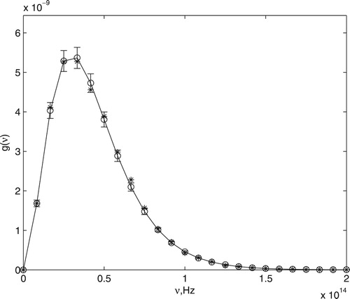The experimental data for $g({\nu }_i)$, simulated between 0 and $2\times {10}^{14}$ Hz, are shown in Figure 1.

Figure 1. Comparison between exact (circle) and simulated (star) power spectrum radiated. The error bar represents the variation coefficient of $5\mathrm{\%}$, for values of ν between 0 and $1\times {10}^{14}$ Hz, and $10\mathrm{\%}$, for values of ν between $1\times {10}^{14}$ Hz and $2\times {10}^{14}$ Hz.

Therefore, the integral equation (12(12) $g(\nu )=\frac{2h{\nu }^3}{c^2}{\int }_0^{\mathrm{\infty }}\frac{1}{e^{h\nu /kT}-1}f(T)\mathrm{d}T\approx {\int }_0^{T_{max}}K(\nu ,T)f(T)\mathrm{d}T.$(12) ) was replaced by the matrix form $\mathbf{g}=\mathbf{K}\mathbf{f}$, in which $\mathbf{K}$ is a matrix of size $25\times 150$, $\mathbf{g}$ is a vector of length 25 and $\mathbf{f}$ is a vector of length 150. Therefore, the problem consists in the determination of $\mathbf{f}$ from $\mathbf{g}$. If this problem is solved without Tikhonov regularization (Equation (2(2) $\begin{array}{rl}{\mathbf{f}}_{\lambda }& =\underset{\mathbf{f}}{min}{\varphi }_{\lambda }(\mathbf{f}),\\ {\mathbf{f}}_{\lambda }& =\{{\mathbf{K}}^T\mathbf{K}+{\lambda }^2(a_0{\mathbf{D}}^{(0)}+a_1{\mathbf{D}}^{(1)}+a_2{\mathbf{D}}^{(2)}){\}}^{-1}{\mathbf{K}}^T\mathbf{g}.\end{array}$(2) ), with $a_0=a_1=a_2=0$), we find a solution that has a reasonably small residual but with a large norm of $\mathbf{f}$. This result cannot be shown in Figure 2, due to the large values in $\mathbf{f}$. Therefore, without the use of the regularization technique an appropriate solution cannot be found.

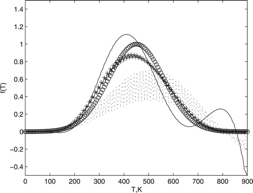
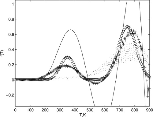
Figure 2. Comparison between exact (circle) and computed temperature distribution. The dotted line was obtained by Equation (2(2) $\begin{array}{rl}{\mathbf{f}}_{\lambda }& =\underset{\mathbf{f}}{min}{\varphi }_{\lambda }(\mathbf{f}),\\ {\mathbf{f}}_{\lambda }& =\{{\mathbf{K}}^T\mathbf{K}+{\lambda }^2(a_0{\mathbf{D}}^{(0)}+a_1{\mathbf{D}}^{(1)}+a_2{\mathbf{D}}^{(2)}){\}}^{-1}{\mathbf{K}}^T\mathbf{g}.\end{array}$(2) ) with $a_0=1$ and $a_1=a_2=0$ and continuous line by Equation (2(2) $\begin{array}{rl}{\mathbf{f}}_{\lambda }& =\underset{\mathbf{f}}{min}{\varphi }_{\lambda }(\mathbf{f}),\\ {\mathbf{f}}_{\lambda }& =\{{\mathbf{K}}^T\mathbf{K}+{\lambda }^2(a_0{\mathbf{D}}^{(0)}+a_1{\mathbf{D}}^{(1)}+a_2{\mathbf{D}}^{(2)}){\}}^{-1}{\mathbf{K}}^T\mathbf{g}.\end{array}$(2) ) with $a_1=1$ and $a_0=a_2=0$. Cross marker is the solution found by Equation (7(7) $\begin{array}{rl}{\mathbf{f}}_{\lambda ,\alpha }& =\underset{\mathbf{f}}{min}{\varphi }_{\lambda ,\alpha }(\mathbf{f}),\\ {\mathbf{f}}_{\lambda ,\alpha }& =\{{\mathbf{K}}^T\mathbf{K}+{\lambda }^2{\mathbf{D}}^{(\alpha )}{\}}^{-1}{\mathbf{K}}^T\mathbf{g},\end{array}$(7) ) with $\alpha =0.6$. All these results were obtained using $\lambda =3.16\times {10}^{-10}$.

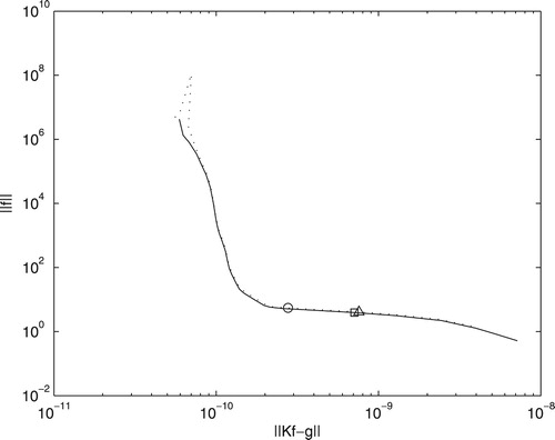
The regularization parameter was chosen initially using the L-curve method (Figure 3). The L-curve is a log–log plot of the norm of a regularized solution versus the norm of the corresponding residual vector. In general, the corner point of the L-curve corresponds to the best value for the regularization parameter. If lower regularization parameter is chosen, there will be an increase in the amplitude of the oscillations. On the other hand, if larger values are considered, then the residual norm increases to values higher than of the experimental error. Then, we can control the solution shape by choosing regularization parameter. For more realistic meaning, the parameter chosen ($3.16\times {10}^{-10}$) was different from the one obtained by L-curve ; however, these values are close together, as we can see in Figure 3 (square symbol).

Figure 3. The L-curve for Equation (2(2) $\begin{array}{rl}{\mathbf{f}}_{\lambda }& =\underset{\mathbf{f}}{min}{\varphi }_{\lambda }(\mathbf{f}),\\ {\mathbf{f}}_{\lambda }& =\{{\mathbf{K}}^T\mathbf{K}+{\lambda }^2(a_0{\mathbf{D}}^{(0)}+a_1{\mathbf{D}}^{(1)}+a_2{\mathbf{D}}^{(2)}){\}}^{-1}{\mathbf{K}}^T\mathbf{g}.\end{array}$(2) ) with $a_0=1$ and $a_1=a_2=0$ (continuous line) and Equation (7(7) $\begin{array}{rl}{\mathbf{f}}_{\lambda ,\alpha }& =\underset{\mathbf{f}}{min}{\varphi }_{\lambda ,\alpha }(\mathbf{f}),\\ {\mathbf{f}}_{\lambda ,\alpha }& =\{{\mathbf{K}}^T\mathbf{K}+{\lambda }^2{\mathbf{D}}^{(\alpha )}{\}}^{-1}{\mathbf{K}}^T\mathbf{g},\end{array}$(7) ) with $\alpha =0.6$ (dotted line). The points marked by the square and the circle correspond to the regularization parameters of $3.16\times {10}^{-10}$ using Equations (2(2) $\begin{array}{rl}{\mathbf{f}}_{\lambda }& =\underset{\mathbf{f}}{min}{\varphi }_{\lambda }(\mathbf{f}),\\ {\mathbf{f}}_{\lambda }& =\{{\mathbf{K}}^T\mathbf{K}+{\lambda }^2(a_0{\mathbf{D}}^{(0)}+a_1{\mathbf{D}}^{(1)}+a_2{\mathbf{D}}^{(2)}){\}}^{-1}{\mathbf{K}}^T\mathbf{g}.\end{array}$(2) ) and (7(7) $\begin{array}{rl}{\mathbf{f}}_{\lambda ,\alpha }& =\underset{\mathbf{f}}{min}{\varphi }_{\lambda ,\alpha }(\mathbf{f}),\\ {\mathbf{f}}_{\lambda ,\alpha }& =\{{\mathbf{K}}^T\mathbf{K}+{\lambda }^2{\mathbf{D}}^{(\alpha )}{\}}^{-1}{\mathbf{K}}^T\mathbf{g},\end{array}$(7) ), respectively. The result obtained by $1.26\times {10}^{-9}$ and $\alpha =0.6$ is shown by triangle symbol.

Using Equation (2(2) $\begin{array}{rl}{\mathbf{f}}_{\lambda }& =\underset{\mathbf{f}}{min}{\varphi }_{\lambda }(\mathbf{f}),\\ {\mathbf{f}}_{\lambda }& =\{{\mathbf{K}}^T\mathbf{K}+{\lambda }^2(a_0{\mathbf{D}}^{(0)}+a_1{\mathbf{D}}^{(1)}+a_2{\mathbf{D}}^{(2)}){\}}^{-1}{\mathbf{K}}^T\mathbf{g}.\end{array}$(2) ) to find $\mathbf{f}$, with $a_0=1$, $a_1=0$ and $a_2=0$, we arrived at an unstable solution. This result is shown in Figure 2 (dotted line) for the regularization parameter which equals to $\lambda =3.16\times {10}^{-10}$. A better result is obtained with $a_0=0$, $a_1=1$ and $a_2=0$ in Equation (2(2) $\begin{array}{rl}{\mathbf{f}}_{\lambda }& =\underset{\mathbf{f}}{min}{\varphi }_{\lambda }(\mathbf{f}),\\ {\mathbf{f}}_{\lambda }& =\{{\mathbf{K}}^T\mathbf{K}+{\lambda }^2(a_0{\mathbf{D}}^{(0)}+a_1{\mathbf{D}}^{(1)}+a_2{\mathbf{D}}^{(2)}){\}}^{-1}{\mathbf{K}}^T\mathbf{g}.\end{array}$(2) ). This result is also shown in Figure 2 (continuous line) for the same regularization parameter. However, it can be observed that the result presented in Figure 2 contains oscillations with very large amplitude, even when the regularization Tikhonov technique (Equation (2(2) $\begin{array}{rl}{\mathbf{f}}_{\lambda }& =\underset{\mathbf{f}}{min}{\varphi }_{\lambda }(\mathbf{f}),\\ {\mathbf{f}}_{\lambda }& =\{{\mathbf{K}}^T\mathbf{K}+{\lambda }^2(a_0{\mathbf{D}}^{(0)}+a_1{\mathbf{D}}^{(1)}+a_2{\mathbf{D}}^{(2)}){\}}^{-1}{\mathbf{K}}^T\mathbf{g}.\end{array}$(2) ), with $a_0=1$ and $a_1=a_2=0$, or $a_1=1$ and $a_0=a_2=0$) with adequate regularization parameter was used. These are the best solutions provided by Equation (2(2) $\begin{array}{rl}{\mathbf{f}}_{\lambda }& =\underset{\mathbf{f}}{min}{\varphi }_{\lambda }(\mathbf{f}),\\ {\mathbf{f}}_{\lambda }& =\{{\mathbf{K}}^T\mathbf{K}+{\lambda }^2(a_0{\mathbf{D}}^{(0)}+a_1{\mathbf{D}}^{(1)}+a_2{\mathbf{D}}^{(2)}){\}}^{-1}{\mathbf{K}}^T\mathbf{g}.\end{array}$(2) ). To improve this, the strategies are (a) remove noise from $\mathbf{g}$; (b) decrease the dimension of the vector f and (c) change numerical quadrature routine. These strategies have already been explored in the literature [2, 3].

This paper proposes a different way. When Equation (7(7) $\begin{array}{rl}{\mathbf{f}}_{\lambda ,\alpha }& =\underset{\mathbf{f}}{min}{\varphi }_{\lambda ,\alpha }(\mathbf{f}),\\ {\mathbf{f}}_{\lambda ,\alpha }& =\{{\mathbf{K}}^T\mathbf{K}+{\lambda }^2{\mathbf{D}}^{(\alpha )}{\}}^{-1}{\mathbf{K}}^T\mathbf{g},\end{array}$(7) ) is used to find $\mathbf{f}$, we have a new parameter, that is α. In this case, with fixed λ ($3.16\times {10}^{-10}$), we can use α to control the amplitude of the oscillations. With $\alpha =0.6$, we find a solution that has a small residual norm as well as oscillations with small amplitude. This result is shown in Figure 2 (cross symbols line). Therefore, the use of Equation (7(7) $\begin{array}{rl}{\mathbf{f}}_{\lambda ,\alpha }& =\underset{\mathbf{f}}{min}{\varphi }_{\lambda ,\alpha }(\mathbf{f}),\\ {\mathbf{f}}_{\lambda ,\alpha }& =\{{\mathbf{K}}^T\mathbf{K}+{\lambda }^2{\mathbf{D}}^{(\alpha )}{\}}^{-1}{\mathbf{K}}^T\mathbf{g},\end{array}$(7) ) instead of Equation (2(2) $\begin{array}{rl}{\mathbf{f}}_{\lambda }& =\underset{\mathbf{f}}{min}{\varphi }_{\lambda }(\mathbf{f}),\\ {\mathbf{f}}_{\lambda }& =\{{\mathbf{K}}^T\mathbf{K}+{\lambda }^2(a_0{\mathbf{D}}^{(0)}+a_1{\mathbf{D}}^{(1)}+a_2{\mathbf{D}}^{(2)}){\}}^{-1}{\mathbf{K}}^T\mathbf{g}.\end{array}$(2) ) led us to a result that is better.

Figure 3 shows the L-curve obtained for $\alpha =0$ (continuous line) and $\alpha =0.6$ (dotted line) for different values of regularization parameter. The corner point with $\alpha =0$ is found when $\lambda =1\times {10}^{-11}$ and with $\alpha =0.6$ is found when λ is close to $3\times {10}^{-11}$. As we can see, the optimal regularization parameter (corner point) is not the same for different values of α. The point marked by circle corresponds to the regularization parameter of $3.16\times {10}^{-10}$ and the triangle symbol indicates the point with regularization parameter of $1.26\times {10}^{-9}$, both with $\alpha =0.6$. The result obtained by $\lambda =3.16\times {10}^{-10}$ and $\alpha =0$ (square symbol) overlaps in L-curve with the result obtained by $\lambda =1.26\times {10}^{-9}$ and $\alpha =0.6$ (triangle symbol). Therefore, both results provide same solution norm and residual norm but with another different feature. Figure 4 shows that the result found with $\lambda =3.16\times {10}^{-10}$ is better than the solution with $\lambda =1.26\times {10}^{-9}$, both with $\alpha =0.6$.

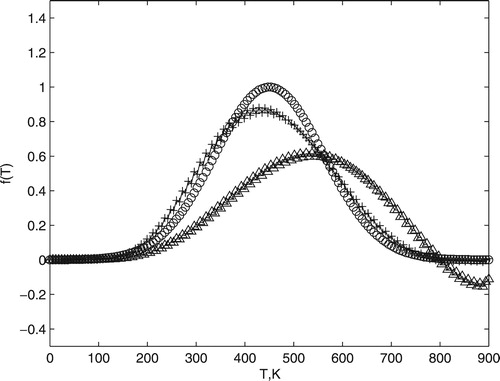
Figure 4. Comparison between exact (circle) and two computed temperature distribution. Cross marker is the solution found by Equation (7(7) $\begin{array}{rl}{\mathbf{f}}_{\lambda ,\alpha }& =\underset{\mathbf{f}}{min}{\varphi }_{\lambda ,\alpha }(\mathbf{f}),\\ {\mathbf{f}}_{\lambda ,\alpha }& =\{{\mathbf{K}}^T\mathbf{K}+{\lambda }^2{\mathbf{D}}^{(\alpha )}{\}}^{-1}{\mathbf{K}}^T\mathbf{g},\end{array}$(7) ) with $\alpha =0.6$ and $\lambda =3.16\times {10}^{-10}$. Triangle marker is the solution found by Equation (7(7) $\begin{array}{rl}{\mathbf{f}}_{\lambda ,\alpha }& =\underset{\mathbf{f}}{min}{\varphi }_{\lambda ,\alpha }(\mathbf{f}),\\ {\mathbf{f}}_{\lambda ,\alpha }& =\{{\mathbf{K}}^T\mathbf{K}+{\lambda }^2{\mathbf{D}}^{(\alpha )}{\}}^{-1}{\mathbf{K}}^T\mathbf{g},\end{array}$(7) ) with $\alpha =0.6$ and $\lambda =1.26\times {10}^{-9}$.

As discussed, one way to improve the result obtained by the Tikhonov method is to decrease the dimension of the vector $\mathbf{f}$. But this is not the strategy used here. The length of the vector $\mathbf{f}$ is large enough to highlight the big oscillations in non-regularized solution and regularized solution with $a_0=1$, $a_1=a_2=0$, as seen in Figure 2. Figure 5 shows that the results obtained with $25\times 150$ dimension of the matrix K and $25\times 300$ dimension of the matrix K are very similar.

Figure 5. The exact temperature distribution (circle) and the results obtained with $25\times 150$ dimension of the matrix K (star) and $25\times 300$ dimension of the matrix K (triangle). All these results were obtained using $\lambda =3.16\times {10}^{-10}$ and $\alpha =0.6$.

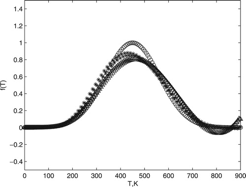
When α is equal to zero, the solution found does not minimize the residual norm (see triangle in Figure 7) with the presence of large oscillations (see dotted line in Figure 2). On the other hand, when α is equal to one, we find a solution which departs from the exact value (see circle in Figure 7) with a oscillation in large frequency (see continuous line in Figure 2). Therefore, there is one α that establishes the good balance between the residual norm and oscillations; this optimum α provides the solution desired.

The choice of α was made using the graphical method. In this case, the Euclidian norm of the first-order derivative of the solution is plotted in Figure 6 for different values of α. We suggest that the minimum of the curve in Figure 6 provides an optimum value of α. In this case, the α chosen (0.6) was different from the one obtained by the mentioned curve. However, the value was close to be predicted. As well as the L-curve was used to get the regularization parameter, which was later refined by comparison between exact and recovered results ; Figure 6 was used to estimate an approximate value of α. In the future, new procedures to determine the fractional order should be explored.

Figure 6. The Euclidian norm of the first-order derivative of the solution obtained by Equation (7(7) $\begin{array}{rl}{\mathbf{f}}_{\lambda ,\alpha }& =\underset{\mathbf{f}}{min}{\varphi }_{\lambda ,\alpha }(\mathbf{f}),\\ {\mathbf{f}}_{\lambda ,\alpha }& =\{{\mathbf{K}}^T\mathbf{K}+{\lambda }^2{\mathbf{D}}^{(\alpha )}{\}}^{-1}{\mathbf{K}}^T\mathbf{g},\end{array}$(7) ) for different values of α, at fixed λ.

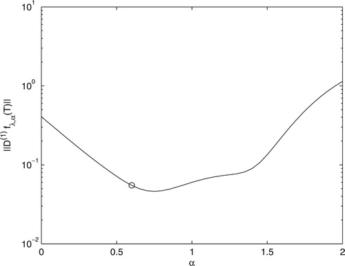
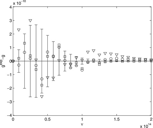
Figure 7. The triangle represents the residual to the result obtained by Equation (2(2) $\begin{array}{rl}{\mathbf{f}}_{\lambda }& =\underset{\mathbf{f}}{min}{\varphi }_{\lambda }(\mathbf{f}),\\ {\mathbf{f}}_{\lambda }& =\{{\mathbf{K}}^T\mathbf{K}+{\lambda }^2(a_0{\mathbf{D}}^{(0)}+a_1{\mathbf{D}}^{(1)}+a_2{\mathbf{D}}^{(2)}){\}}^{-1}{\mathbf{K}}^T\mathbf{g}.\end{array}$(2) ) with $a_0=1$ and $a_1=a_2=0$ and the circle represents the residual to the result obtained by Equation (2(2) $\begin{array}{rl}{\mathbf{f}}_{\lambda }& =\underset{\mathbf{f}}{min}{\varphi }_{\lambda }(\mathbf{f}),\\ {\mathbf{f}}_{\lambda }& =\{{\mathbf{K}}^T\mathbf{K}+{\lambda }^2(a_0{\mathbf{D}}^{(0)}+a_1{\mathbf{D}}^{(1)}+a_2{\mathbf{D}}^{(2)}){\}}^{-1}{\mathbf{K}}^T\mathbf{g}.\end{array}$(2) ) with $a_1=1$ and $a_0=a_2=0$. The square is the result to Equation (7(7) $\begin{array}{rl}{\mathbf{f}}_{\lambda ,\alpha }& =\underset{\mathbf{f}}{min}{\varphi }_{\lambda ,\alpha }(\mathbf{f}),\\ {\mathbf{f}}_{\lambda ,\alpha }& =\{{\mathbf{K}}^T\mathbf{K}+{\lambda }^2{\mathbf{D}}^{(\alpha )}{\}}^{-1}{\mathbf{K}}^T\mathbf{g},\end{array}$(7) ) with $\alpha =0.6$. The error bar represents the variation coefficient of $5\mathrm{\%}$, for values of ν between 0 and $1\times {10}^{14}$ Hz, and $10\mathrm{\%}$, for values of ν between $1\times {10}^{14}$ and $2\times {10}^{14}$ Hz.

In Figure 7, the triangle symbol represents the residual in the results obtained by Equation (2(2) $\begin{array}{rl}{\mathbf{f}}_{\lambda }& =\underset{\mathbf{f}}{min}{\varphi }_{\lambda }(\mathbf{f}),\\ {\mathbf{f}}_{\lambda }& =\{{\mathbf{K}}^T\mathbf{K}+{\lambda }^2(a_0{\mathbf{D}}^{(0)}+a_1{\mathbf{D}}^{(1)}+a_2{\mathbf{D}}^{(2)}){\}}^{-1}{\mathbf{K}}^T\mathbf{g}.\end{array}$(2) ) with $a_0=1$ and $a_1=a_2=0$ and circle symbol represents the residual to the result obtained by Equation (2(2) $\begin{array}{rl}{\mathbf{f}}_{\lambda }& =\underset{\mathbf{f}}{min}{\varphi }_{\lambda }(\mathbf{f}),\\ {\mathbf{f}}_{\lambda }& =\{{\mathbf{K}}^T\mathbf{K}+{\lambda }^2(a_0{\mathbf{D}}^{(0)}+a_1{\mathbf{D}}^{(1)}+a_2{\mathbf{D}}^{(2)}){\}}^{-1}{\mathbf{K}}^T\mathbf{g}.\end{array}$(2) ) with $a_1=1$ and $a_0=a_2=0$. It is worth remembering that these results can be obtained using Equation (7(7) $\begin{array}{rl}{\mathbf{f}}_{\lambda ,\alpha }& =\underset{\mathbf{f}}{min}{\varphi }_{\lambda ,\alpha }(\mathbf{f}),\\ {\mathbf{f}}_{\lambda ,\alpha }& =\{{\mathbf{K}}^T\mathbf{K}+{\lambda }^2{\mathbf{D}}^{(\alpha )}{\}}^{-1}{\mathbf{K}}^T\mathbf{g},\end{array}$(7) ) with $\alpha =0$ and Equation (7(7) $\begin{array}{rl}{\mathbf{f}}_{\lambda ,\alpha }& =\underset{\mathbf{f}}{min}{\varphi }_{\lambda ,\alpha }(\mathbf{f}),\\ {\mathbf{f}}_{\lambda ,\alpha }& =\{{\mathbf{K}}^T\mathbf{K}+{\lambda }^2{\mathbf{D}}^{(\alpha )}{\}}^{-1}{\mathbf{K}}^T\mathbf{g},\end{array}$(7) ) with $\alpha =1$, respectively. The error bar shown in Figure 7 represents the variation coefficient of $5\mathrm{\%}$, for values of ν between 0 and $1\times {10}^{14}$ Hz, and $10\mathrm{\%}$, for values of ν between $1\times {10}^{14}$ and $2\times {10}^{14}$ Hz.

Finally, we can observe in Figures 2 and 7 that for $\alpha =0$, the retrieved values of $g(\nu )$ from $f(T)$ are not within experimental error bar and that $f(T)$ function has great oscillations. For $\alpha =1$, the recovered values of $g(\nu )$ are within experimental error bar for small values of ν and are without experimental error bar for big values of ν. The result found for $f(T)$, with $\alpha =1$, contains a big oscillation in large frequencies. All these results were obtained using Equation (7(7) $\begin{array}{rl}{\mathbf{f}}_{\lambda ,\alpha }& =\underset{\mathbf{f}}{min}{\varphi }_{\lambda ,\alpha }(\mathbf{f}),\\ {\mathbf{f}}_{\lambda ,\alpha }& =\{{\mathbf{K}}^T\mathbf{K}+{\lambda }^2{\mathbf{D}}^{(\alpha )}{\}}^{-1}{\mathbf{K}}^T\mathbf{g},\end{array}$(7) ) and $\lambda =3.16\times {10}^{-10}$. For $\alpha =0.6$ and $\lambda =3.16\times {10}^{-10}$, the difference between simulated ${\mathbf{g}}^{\exp }$ and recovered ${\mathbf{g}}^{\mathrm{cal}}$ are within experimental error bar and with small oscillations in $f(T)$ function.

Other functions to $f(T)$ were used to study efficiency of the proposed method: (14) $\begin{array}{rl}f(T)& =\frac{\tanh \left(\frac{T-250}{20}\right)+\tanh \left(\frac{-T+550}{20}\right)}{2},\end{array}$(14) (15) $\begin{array}{rl}f(T)& =0.3\exp \left(\frac{-(T-350{)}^2}{4500}\right)+0.7\exp \left(\frac{-(T-750{)}^2}{7500}\right).\end{array}$(15) For these cases, the results are shown in Figures 8 and 9, respectively. The best results were found when 0.6 and 0.5 were considered for the parameter α. The regularization parameter that was used were $1.95\times {10}^{-10}$ and $4.47\times {10}^{-10}$, respectively. The variable range, the dimension matrix and the standard deviation were taken as before. Again, the proposed modification allows to achieve results that have a small norm of the solution and only very few oscillations than when using $\alpha =0$ or $\alpha =1$ (usual model).

Figure 8. The exact temperature distribution (Equation (14(14) $\begin{array}{rl}f(T)& =\frac{\tanh \left(\frac{T-250}{20}\right)+\tanh \left(\frac{-T+550}{20}\right)}{2},\end{array}$(14) )) is shown with circle marker and compared to different computed results. The dotted line was obtained by Equation (2(2) $\begin{array}{rl}{\mathbf{f}}_{\lambda }& =\underset{\mathbf{f}}{min}{\varphi }_{\lambda }(\mathbf{f}),\\ {\mathbf{f}}_{\lambda }& =\{{\mathbf{K}}^T\mathbf{K}+{\lambda }^2(a_0{\mathbf{D}}^{(0)}+a_1{\mathbf{D}}^{(1)}+a_2{\mathbf{D}}^{(2)}){\}}^{-1}{\mathbf{K}}^T\mathbf{g}.\end{array}$(2) ) with $a_0=1$ and $a_1=a_2=0$ and continuous line by Equation (2(2) $\begin{array}{rl}{\mathbf{f}}_{\lambda }& =\underset{\mathbf{f}}{min}{\varphi }_{\lambda }(\mathbf{f}),\\ {\mathbf{f}}_{\lambda }& =\{{\mathbf{K}}^T\mathbf{K}+{\lambda }^2(a_0{\mathbf{D}}^{(0)}+a_1{\mathbf{D}}^{(1)}+a_2{\mathbf{D}}^{(2)}){\}}^{-1}{\mathbf{K}}^T\mathbf{g}.\end{array}$(2) ) with $a_1=1$ and $a_0=a_2=0$. Cross marker is the solution found by Equation (7(7) $\begin{array}{rl}{\mathbf{f}}_{\lambda ,\alpha }& =\underset{\mathbf{f}}{min}{\varphi }_{\lambda ,\alpha }(\mathbf{f}),\\ {\mathbf{f}}_{\lambda ,\alpha }& =\{{\mathbf{K}}^T\mathbf{K}+{\lambda }^2{\mathbf{D}}^{(\alpha )}{\}}^{-1}{\mathbf{K}}^T\mathbf{g},\end{array}$(7) ) with $\alpha =0.6$. All these results were obtained using $\lambda =1.95\times {10}^{-10}$.

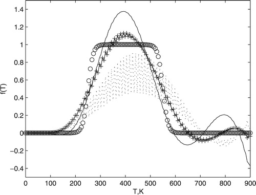
Figure 9. The circle marker is the exact temperature distribution (Equation (15(15) $\begin{array}{rl}f(T)& =0.3\exp \left(\frac{-(T-350{)}^2}{4500}\right)+0.7\exp \left(\frac{-(T-750{)}^2}{7500}\right).\end{array}$(15) )). The dotted line was obtained by Equation (2(2) $\begin{array}{rl}{\mathbf{f}}_{\lambda }& =\underset{\mathbf{f}}{min}{\varphi }_{\lambda }(\mathbf{f}),\\ {\mathbf{f}}_{\lambda }& =\{{\mathbf{K}}^T\mathbf{K}+{\lambda }^2(a_0{\mathbf{D}}^{(0)}+a_1{\mathbf{D}}^{(1)}+a_2{\mathbf{D}}^{(2)}){\}}^{-1}{\mathbf{K}}^T\mathbf{g}.\end{array}$(2) ) with $a_0=1$ and $a_1=a_2=0$ and continuous line by Equation (2(2) $\begin{array}{rl}{\mathbf{f}}_{\lambda }& =\underset{\mathbf{f}}{min}{\varphi }_{\lambda }(\mathbf{f}),\\ {\mathbf{f}}_{\lambda }& =\{{\mathbf{K}}^T\mathbf{K}+{\lambda }^2(a_0{\mathbf{D}}^{(0)}+a_1{\mathbf{D}}^{(1)}+a_2{\mathbf{D}}^{(2)}){\}}^{-1}{\mathbf{K}}^T\mathbf{g}.\end{array}$(2) ) with $a_1=1$ and $a_0=a_2=0$. Cross marker is the solution found by Equation (7(7) $\begin{array}{rl}{\mathbf{f}}_{\lambda ,\alpha }& =\underset{\mathbf{f}}{min}{\varphi }_{\lambda ,\alpha }(\mathbf{f}),\\ {\mathbf{f}}_{\lambda ,\alpha }& =\{{\mathbf{K}}^T\mathbf{K}+{\lambda }^2{\mathbf{D}}^{(\alpha )}{\}}^{-1}{\mathbf{K}}^T\mathbf{g},\end{array}$(7) ) with $\alpha =0.6$. All these results were achieved using $\lambda =4.47\times {10}^{-10}$.

4. Conclusions

In the present study, for the first time, we employed the norm of the fractional derivative order as a restriction in the functional proposed originally by Tikhonov. The question about how fractional order has an effect on the solution $\mathbf{f}$ at λ fixed was discussed. This work shows that the proposed modification is more flexible than the original method, with better results using $\alpha =0.6$ or $\alpha =0.5$ instead of $\alpha =0$ or $\alpha =1$. This result was achieved even with the presence of experimental errors (variation coefficient of $5\mathrm{\%}$ and $10\mathrm{\%}$) in simulated data.

Disclosure statement

No potential conflict of interest was reported by the author(s).

ORCID

Nelson H. T. Lemes http://orcid.org/0000-0002-1309-542X

José P. C. dos Santos http://orcid.org/0000-0002-4161-1786

João P. Braga http://orcid.org/0000-0002-2869-7079

Additional information

Funding

This study was financed in part by the Coordenação de Aperfeiçoamento de Pessoal de Nível Superior – Brasil (CAPES) – Finance Code 001 and FAPEMIG.

References

- Tikhonov AN, Goncharsky AV, Stepanov VV, et al. Numerical methods for the solution of ill-posed problems. Dordrecht: Springer Netherlands; 1995.
- Phillips DL. A technique for the numerical solution of certain integral equations of the first kind. J ACM. 1962;9(1):84–97. doi: 10.1145/321105.321114
- Tikhonov AN. Translated in ‘solution of incorrectly formulated problems and the regularization method’. Soviet Math Dokl. 1963;4(4):1035–1038.
- Hansen PC. Rank-deficient and discrete ill-posed problems: numerical aspects of linear inversion. Philadelphia (PA): Society for Industrial and Applied Mathematics; 1998.
- Vogel CR. Computational methods for inverse problems. Philadelphia (PA): Society for Industrial and Applied Mathematics; 2002.
- Lemes NHT, Braga JP, Belchior JC. Spherical potential energy function from second virial coefficient using Tikhonov regularization and truncated singular value decomposition. Chem Phys Lett. 1998;296(3–4):233–238. doi: 10.1016/S0009-2614(98)01042-2
- Braga JP. Numerical comparison between Tikhonov regularization and singular value decomposition methods using the L curve criterion. J Math Chem. 2001;29(2):151–161. doi: 10.1023/A:1010983230567
- Podlubny I. Fractional differential equations: an introduction to fractional derivatives, fractional differential equations, some methods of their solution and some of their applications. San Diego (CA): Academic Press; 1999.
- De Oliveira EC, Machado JAT. A review of definitions for fractional derivatives and integral. Math Probl Eng. 2014;2014:1–6. doi: 10.1155/2014/238459
- Sun H, Zhang Y, Baleanu D, et al. A new collection of real world applications of fractional calculus in science and engineering. Commun Nonlinear Sci Numer Simul. 2018;64:213–231. doi: 10.1016/j.cnsns.2018.04.019
- Oldham KB, Spanier J. The fractional calculus: integrations and differentiations of arbitraryorder. New York (NY): Academic Press; 1974.
- Lemes NHT, Santos JPCD, Braga JP. A generalized Mittag–Leffer function to describe nonexponential chemical effects. Appl Math Model. 2016;40(17–18):7971–7976. doi: 10.1016/j.apm.2016.04.021
- Bojarski NN. Inverse black body radiation. IEEE Trans Antennas Propag. 1982;30(4):778–780. doi: 10.1109/TAP.1982.1142844
- FengMin J, XianXi D. A new solution method for black-body radiation inversion and the solar area-temperature distribution. Sci China Phys Mech Astron. 2011;54(11):2097–2102. doi: 10.1007/s11433-011-4514-7
- Xu Q, Zheng X, Li Z, et al. Absolute spectral radiance responsivity calibration of sun photometers. Rev Sci Instrum. 2010;81(3):033103. doi: 10.1063/1.3331459
- Nanxian C. A new method for inverse black body radiation problem. Chin Phys Lett. 1987;4(8):337–340. doi: 10.1088/0256-307X/4/8/001
- Nanxian C, Guangyin L. Theoretical investigation on the inverse black body radiation problem. IEEE Trans Antennas Propag. 1990;38(8):1287–1290. doi: 10.1109/8.56968
- Nanxian C. Modified möbius inverse formula and its applications in physics. Phys Rev Lett. 1990;64(11):1193–1195.
- Sun X, Jaggard DL. The inverse black body radiation problem: a regularization solution. J Appl Phys. 1987;62(11):4382–4386. doi: 10.1063/1.339072
- Dou L, Hodgson RJW. Application of the regularization method to the inverse black body radiation problem. IEEE Trans Antennas Propag. 1992;40(10):1249–1253. doi: 10.1109/8.182459
- Li HY. Solution of inverse black body radiation problem with conjugate gradient method. IEEE Trans Antennas Propag. 2005;53(5):1840–1842. doi: 10.1109/TAP.2005.846814
- Lemes NHT, Sebastio RCO, Braga JP. Potential energy function from second virial data using sensitivity analysis. Inverse Probl Sci Eng. 2006;14(6):581–587. doi: 10.1080/17415970600573353
- Riele HJJ. A program for solving first kind Fredholm integral equations by means of regularization. Comput Phys Commun. 1985;36(4):423–432. doi: 10.1016/0010-4655(85)90032-3