Identification of inelastic parameters of the AISI 304 stainless steel: a multi-test optimization strategy

ABSTRACT

The AISI 304 stainless steel has largely been used in industry owing to its good formability characteristics. Therefore, the use of proper material parameters is essential for a successful numerical simulation of forming operations. Within this framework, this work addresses a parameter identification strategy using strategies based on multiple mechanical tests – a multi-test optimization scheme. The technique is used to determine isotropic hardening parameters of the AISI 304 steel using tensile tests of specimens of different geometries. The proposed method makes possible to obtain a representative set of material parameters taking into account the material response up to macroscopic failure. The study shows that the technique provides a minimum improvement of 30.43% in the global error function when comparing against single test results.

Keywords:

• AISI 304 stainless steel
• parameter identification
• optimization

2010 Mathematics Subject Classifications:

• 74S05
• 74P99

1. Introduction

The design strategies of products and components, including manufacturing processes, experienced a significant change in the last decade. Computer aided engineering (CAE) systems, in special commercial packages devoted to metal forming simulation, have become essential tools to new developments. Notwithstanding, the success of numerical simulations of forming operations requires a proper definition of inelastic parameters (i.e. accuracy of the numerical predictions is directly dependent upon the material data used in the simulations). In general, identification of such parameters can use either curve fitting of experimental data or inverse problem techniques. The former consists of fitting a selected equation to fundamental measures (e.g. stresses, strains, etc.) using least-square or other mathematical method, whereas the latter determines the inelastic parameters by combining optimization-based strategies and global measures (e.g. loads, displacements, etc.). This work is inserted within this framework and aims to discuss use of inverse problem techniques to determine inelastic parameters of the AISI 304 stainless steel.

Curve fitting strategies have been largely used to determine inelastic parameters of stainless steels. For instance, Samuel et al. [1,2] discussed the suitability of the classical Hollomon [3], Swift [4] and Ludwigson [5] stress–strain relations to describe the plastic behaviour of the AISI 316 stainless steel at room temperature. The authors conclude that Swift's equation was able to adequately represent hardening evolution. A three-stage description of the yield stress behaviour approximated by Hollomon's equation was proposed by Kashyap and Tangri [6] for the AISI 316L stainless steel. Calibration techniques based on tensile tests were adopted in their study. The strain hardening evolution of the duplex DIN 1.4462 stainless steel alloy was investigated by Hertelé et al. [7], who proposed a two-stage hardening model based on the Ramberg–Osgood equation [8]. Based on micromechanical concepts, El-Magd [9] derived a phenomenological yield stress law also known as modified Voce [10] equation. A good fit was reported for the austenitic stainless steel X8CrNiMoNb16-16. Harth et al. [11] presented a strategy using tension, tension-compression and creep tests to determine inelastic parameters for the AINSI SS316 stainless steel at high temperature. The authors proposed a combined technique based on statistical analysis and design of experiments with the objective of handling variations of the measured data. Haghdadi et al. [12] proposed a new hardening equation derived from mechanisms of dislocation theory. Curve fitting of micromechanic measures was also adopted to obtain parameters for the LDX 2101 duplex stainless steel.

It is noteworthy that curve fitting strategies make possible to achieve a clear physical perception of the interaction between parameters and their intrinsic relation with the constitutive model. However, this technique restricts application to uniform stress and strain conditions which prompt plastic deformations smaller than those typical of metal forming operations.

Identification schemes using inverse problem techniques, in especial optimization-based strategies, make possible to expand analysis over wider range of plastic deformation using complex hardening descriptions under triaxial stress states. In general, these methods compare global experimental data with results obtained from numerical simulations or other approximate solutions. The literature shows a growing number of works featuring parameter identification using such techniques, which in general focus on material modelling (e.g. damaged formulations, anisotropic materials, etc.) and development of optimization strategies (hybrid schemes, multi-information methods, etc.). For instance, Mahnken [13] addressed identification of inelastic parameters based on load–elongation curves of tensile tests for Gurson-type and Rousselier-type damage models using a gradient-based descent method. Wang and Wu [14] discussed the identification of hardening parameters for the 20MnB5 steel using spherical indentation experiment and Bayesian model updating approach. Pacheco et al. [15] also adopted a Bayesian approach to the identification of hardening parameters for the Aluminium alloy AA 6060 T66 based on a three-point bending test of a thin-walled tube. Vaz Jr. et al. [16] proposed a hybrid scheme combining particle swarm optimization and the Nelder–Mead method to the identification of hardening and damage parameters for Lemaitre-type and Gurson-type damage models.

Inverse problem techniques have also been applied to parameter identification of constitutive models other than metallic materials. For instance, Carniel et al. [17] used particle swarm optimization to determine inelastic parameters for the High Density Polyethylene (HDPE) and Isostatic Polypropylene (iPP) associated with a viscoelastic viscoplastic constitutive model. A hybrid genetic algorithm was used by Jin et al. [18] to identification soil parameters in geotechnical fields.

In order to ensure a broader range of validity, the inverse problem must account for as much information as possible. Identification of kinematic and isotropic hardening parameters for cyclic elastoplasticity associated with the Chaboche–Rousselier and Prager models presented by Yoshida et al. [19] is a typical example of this approach. The authors used approximate solutions for uniaxial tensile tests and bending tests associated with a multipoint approximation technique in conjunction with sequential quadratic programming (SQP). Multiple experimental information was also used by Ponthot and Kleinermann [20], who correlated tensile loads and variations of the specimen diameter with displacements to determine hardening variables of a low alloy steel. The authors used in cascade several gradient-based optimization techniques aiming to improve robustness and accuracy of the identification method. A correlation between variations of the specimen diameter, elongation and tensile loads was also adopted by Vaz Jr. et al. [21] to determine hardening parameters for two distinct micromechanical-based phenomenological hardening laws. The authors also concluded in a separate study that parameter identification using optimization-based identification schemes provided better approximations than curve-fitting strategies for the AISI 304 stainless steel [22]. In recent years, digital image correlation has emerged as an important tool to identification of material parameters. The method uses full-field measurements and broadens the information available to the identification strategy [23]. The application of this technique to the identification of material parameters associated with elastic-(visco)plastic materials is a new endeavour, as pointed out by Martins et al. [24].

This work addresses the identification of inelastic parameters based on multiple mechanical tests using optimization techniques. The use of multiple tests aims at a better compliance of the constitutive model and corresponding hardening description using simple experimental settings. The article is organized as follows: Section 2 introduces the optimization technique to determine inelastic parameters. Section 3 illustrates application and Section 4 highlights the main conclusion. An appendix was also included to describe aspects of the plasticity model, kinematic formulation and finite element discretization of the boundary value problem.

2. Parameter identification and the optimization strategy

Despite the common practice of finding inelastic parameters based on single mechanical tests, the phenomenological character of most plasticity models and hardening laws may lead to limitations and inaccuracies (to be demonstrated in Section 3.2). In order to achieve more accurate numerical predictions over a wider range of inelastic deformation, the optimization problem must account for as much information as possible. Therefore, this work proposes a new strategy to determine material parameters based on multiple mechanical tests and/or tests using specimens of different geometrical configurations.

The problem of finding the best set of material parameters based on multiple mechanical tests recommends formulations using specific optimization schemes. The proposed strategy accounts for two objective functions associated with two different sets of design variables and reference measures. The general principles of the proposed scheme are as follows:

1. There exists a set of parameters, ${\mathit{p}}_s^{min}$, which best approximates an individual mechanical test ‘s’, i.e. it provides the minimum possible error function (fitness/objective function), $g_s^{min}({\mathit{p}}_s^{min})$, for each individual test.

2. The best set of parameters for an individual test, ${\mathit{p}}_s^{min}$, does not necessarily constitutes the best set for all other mechanical tests. This is particularly relevant when using phenomenological material descriptions.

3. A mean global error function, G, can be determined by comparing the individual fitness, $g_s(\mathit{p},{\lambda }_s)$, computed with a common set of parameters used in all mechanical tests, $\mathit{p}$, and individual weight, ${\lambda }_s$, with the best individual fitness of each test, $g_s^{min}$, indicated in item (i).

4. Minimization of the mean global error, G, makes possible to find the set of material parameters which better approximate all mechanical tests simultaneously.

The multi-test strategy comprises two distinct stages: the first stage determines the best possible error function for each test, $g_s^{min}$, whereas the second stage solves an optimization problem for the best set of inelastic parameters, $\mathit{p}$, and weights, $\mathit{\lambda }$.

2.1. Stage 1: parameter identification of individual tests

The first stage determines the minimum possible objective function, $g_s^{min}$, for each individual test ‘s’. The number of mechanical tests is designated $n_s$. The initial optimization problem accounts for experimental data obtained from each test, as (1) $\begin{array}{lll}\text{Minimize}& {\displaystyle g_s(\mathit{p})}& \mathit{p}\in R^{n_p}\\ \text{Such that}& p_i^{\inf }\le p_i\le p_i^{\sup }& i=1,\dots ,n_p\end{array}$(1) where $g_s(\mathit{p})$ and $\mathit{p}=[p_1{p}_2\cdots p_i\cdots p_{n_p}{]}^T$ are the objective function (fitness) and design vector for the mechanical test ‘s’, respectively. The number of material parameters is $n_p$, whereas $p_i^{\inf }$ and $p_i^{\sup }$ are lateral constraints and represents the minimum and maximum values of a design variable $p_i$. In this work, the individual fitness, $g_s(\mathit{p})$, represents a quadratic relative error measure between the experimental and numerical load of a mechanical test ‘s’, (2) $g_s\left(\mathit{p}\right)=\sqrt{\frac{1}{N_s}\sum _{j=1}^{N_s}{\left(\frac{R_{s,j}^{Exp}-R{\left(\mathit{p}\right)}_{s,j}^{Num}}{R_{s,j}^{Exp}}\right)}^2},$(2) in which $R_s^{Exp}$ is the experimental tensile load curve measured for each mechanical test ‘s’, $R(\mathit{p}{)}_s^{Num}$ is the corresponding numerical tensile load computed using the material parameters $\mathit{p}$ and $N_s$ is the total number of experimental points in the load curve for the mechanical test ‘s’, and the subscript ‘j’ in Equation (2(2) $g_s\left(\mathit{p}\right)=\sqrt{\frac{1}{N_s}\sum _{j=1}^{N_s}{\left(\frac{R_{s,j}^{Exp}-R{\left(\mathit{p}\right)}_{s,j}^{Num}}{R_{s,j}^{Exp}}\right)}^2},$(2) ) represents individual values of the experimental and numerical load curves. Noticeably, $R(\mathit{p}{)}_s^{Num}$ is obtained by solving the direct problem using the finite element approximation summarised in Appendix.

The optimization problem defined in Equation (1(1) $\begin{array}{lll}\text{Minimize}& {\displaystyle g_s(\mathit{p})}& \mathit{p}\in R^{n_p}\\ \text{Such that}& p_i^{\inf }\le p_i\le p_i^{\sup }& i=1,\dots ,n_p\end{array}$(1) ) is solved for each mechanical test ‘s’, giving rise to sets of material data, ${\mathit{p}}_s^{min}$, and individual fitness, $g_s^{min}({\mathit{p}}_s^{min})$, which can be expressed in vector notation as ${\mathit{P}}^{min}=[{\mathit{p}}_1^{min}{\mathit{p}}_2^{min}\cdots {\mathit{p}}_s^{min}\cdots {\mathit{p}}_{n_s}^{min}{]}^T$ and ${\mathit{G}}^{min}=[g_1^{min}{g}_2^{min}\cdots g_s^{min}\cdots g_{n_s}^{min}{]}^T$, respectively.

It is important to mention that, owing to the phenomenological character of the material model, there is no guarantee that any individual set of material parameters, ${\mathit{p}}_s^{min}$, obtained at this point can provide the best approximation to all mechanical tests simultaneously. Therefore, the next stage constitutes solution of an optimization problem defined with the objective of finding the best overall set of material parameters.

2.2. Stage 2: parameter identification of simultaneous tests

The optimization problem proposed in this stage accounts for two objective functions, which are associated with the experimental loading curve for each test, $R_s^{Exp}$, and best possible error function for each test, $g_s^{min}$ (determined in Stage 1).

Parameter identification of composed tests: The problem combines the individual fitness, $g_s(\mathit{p})$, into a global objective function by means of a linear combination. The optimization problem can be formulated in similar fashion as Equation (1(1) $\begin{array}{lll}\text{Minimize}& {\displaystyle g_s(\mathit{p})}& \mathit{p}\in R^{n_p}\\ \text{Such that}& p_i^{\inf }\le p_i\le p_i^{\sup }& i=1,\dots ,n_p\end{array}$(1) ), (3) $\begin{array}{lll}\text{Minimize}& {\displaystyle g(\mathit{p},\mathit{\lambda })=\sum _{s=1}^{n_s}{\lambda }_s{g}_s(\mathit{p})}& \mathit{p}\in R^{n_p}\\ \text{Such that}& p_i^{\inf }\le p_i\le p_i^{\sup }& i=1,\dots ,n_p\end{array}$(3) where $\mathit{p}$ are the design variables, $g(\mathit{p},\mathit{\lambda })$ is the composed objective function, $g_s(\mathit{p})$ is the individual fitness defined in Equation (2(2) $g_s\left(\mathit{p}\right)=\sqrt{\frac{1}{N_s}\sum _{j=1}^{N_s}{\left(\frac{R_{s,j}^{Exp}-R{\left(\mathit{p}\right)}_{s,j}^{Num}}{R_{s,j}^{Exp}}\right)}^2},$(2) ) and $\mathit{\lambda }=[{\lambda }_1{\lambda }_2\cdots {\lambda }_s\cdots {\lambda }_{n_s}{]}^T$ is the set of weights which establishes the degree of influence of each mechanical test in the computation of the material parameters $\mathit{p}$. Noticeably, $\mathit{\lambda }$ is constant for the optimization problem defined by Equation (3(3) $\begin{array}{lll}\text{Minimize}& {\displaystyle g(\mathit{p},\mathit{\lambda })=\sum _{s=1}^{n_s}{\lambda }_s{g}_s(\mathit{p})}& \mathit{p}\in R^{n_p}\\ \text{Such that}& p_i^{\inf }\le p_i\le p_i^{\sup }& i=1,\dots ,n_p\end{array}$(3) ) and must satisfy the condition $\sum _{s=1}^{n_s}{\lambda }_s=1$.

Finding the best set of weight parameters, ${\mathit{\lambda }}^{min}$. The global optimization problem requires simultaneous determination of weight parameters ${\mathit{\lambda }}^{min}=[{\lambda }_1^{min}{\lambda }_2^{min}\cdots {\lambda }_s^{min}\cdots {\lambda }_{n_s}^{min}{]}^T$ which yield the best approximation of $g_s(\mathit{p})$ to $g_s^{min}$ for each corresponding mechanical test ‘s’. The problem is solved with weight functions $\mathit{\lambda }$ as design variables, as (4) $\begin{array}{lcl}\text{Minimize}& {\displaystyle G(\mathit{\lambda })}& \mathit{\lambda }\in R^{n_s}\\ \text{Such that}& {\displaystyle 0\le {\lambda }_s\le 1}& s=1,\dots ,n_s\\ & {\displaystyle \sum _{s=1}^{n_s}{\lambda }_s=1}& \end{array}$(4) in which $G(\mathit{\lambda })$ is the mean global error, (5) $G(\mathit{\lambda })\equiv G[g_s(\mathit{p},{\lambda }_s)]=\sqrt{\frac{1}{n_s}\sum _{s=1}^{n_s}{\left[\frac{g_s^{min}-g_s(\mathit{p},{\lambda }_s)}{g_s^{min}}\right]}^2},$(5) which expresses a quadratic relative error between the best approximation, $g_s^{min}$, for each mechanical test (solution of Equation (1(1) $\begin{array}{lll}\text{Minimize}& {\displaystyle g_s(\mathit{p})}& \mathit{p}\in R^{n_p}\\ \text{Such that}& p_i^{\inf }\le p_i\le p_i^{\sup }& i=1,\dots ,n_p\end{array}$(1) )) and individual fitness, $g_s(\mathit{p},{\lambda }_s)$, obtained by solving the optimization problem established in Equation (3(3) $\begin{array}{lll}\text{Minimize}& {\displaystyle g(\mathit{p},\mathit{\lambda })=\sum _{s=1}^{n_s}{\lambda }_s{g}_s(\mathit{p})}& \mathit{p}\in R^{n_p}\\ \text{Such that}& p_i^{\inf }\le p_i\le p_i^{\sup }& i=1,\dots ,n_p\end{array}$(3) ). It is important to mention that there is a unique relation between the individual fitness and weight for each mechanical test, $g_s(\mathit{p},{\lambda }_s)$ $\iff {\lambda }_s$, and, therefore, the mean global error is henceforth referred to as $G(\mathit{\lambda })$. Table 1 presents the optimization algorithm.

Table 1. Optimization strategy to determine material parameters, $\mathit{p}$, and weights, $\mathit{\lambda }$.

(i)	Parameter identification for each individual mechanical test, ‘s’:
	WHILE $s⩽n_s$ DO
	Find individual set of parameters, ${\mathit{p}}_s$, and respective objective function, $g_s$
	Minimize ${\displaystyle g_s({\mathit{p}}_s)=\sqrt{{\displaystyle \frac{1}{N_s}}\sum _{i=1}^{N_s}{\left[{\displaystyle \frac{R_{s,i}^{Exp}-R^{Num}({\mathit{p}}_s{)}_i}{R_{s,i}^{Exp}}}\right]}^2}}$
	$g_s^{min}\leftarrow g_s({\mathit{p}}_s)$ where ${\mathit{p}}_s=[p_1^s{p}_2^s\cdots p_i^s\cdots p_{n_p}^s{]}^T$
	END WHILE
	Get set of best individual fitness, ${\mathit{g}}^{min}=[g_1^{min}{g}_2^{min}\cdots g_s^{min}\cdots g_{n_s}^{min}{]}^T$
(ii)	Determine global weights, $\mathit{\lambda }$, which cause $g_s(\mathit{p})$ to best approximate individual $g_s^{min}$:
	Define initial estimate ${\mathit{\lambda }}^{(0)}=[{\lambda }_1^{(0)}{\lambda }_2^{(0)}\cdots {\lambda }_s^{(0)}\cdots {\lambda }_{n_s}^{(0)}{]}^T$
	WHILE ${\varphi }_d^{(k)}>TO{L}_d$ DO
	Find new ${\mathit{\lambda }}^{(k)}$ from minimizing $G({\mathit{\lambda }}^{(k)})$
	Find individual $g_s({\mathit{p}}^{(k)})$ for ${\mathit{\lambda }}^{(k)}$ from parameter identification
	Minimize ${\displaystyle g({\mathit{p}}^{(k)},{\mathit{\lambda }}^{(k)})=\sum _{s=1}^{n_s}{\lambda }_s^{(k)}{g}_s({\mathit{p}}^{(k)})}$
	${\mathit{p}}^{(k+1)}\leftarrow {\mathit{p}}^{(k)}$
	$\mathit{g}({\mathit{p}}^{(k+1)})\leftarrow [g_1({\mathit{p}}^{(k)})g_2({\mathit{p}}^{(k)})\cdots g_s({\mathit{p}}^{(k)})\cdots g_{n_s}({\mathit{p}}^{(k)}){]}^T$
	Minimize ${\displaystyle G({\mathit{\lambda }}^{(k)})=\sqrt{{\displaystyle \frac{1}{n_s}}\sum _{s=1}^{n_s}{\left[{\displaystyle \frac{g_s^{min}-g_s({\mathit{p}}^{(k+1)},{\lambda }_s^{(k)})}{g_s^{min}}}\right]}^2}}$
	Compute convergence index, ${\varphi }_d({\mathit{\lambda }}^{(k)})$, for the global optimization scheme
	${\mathit{\lambda }}^{(k+1)}\leftarrow {\mathit{\lambda }}^{(k)}$
	$k\leftarrow k+1$
	END WHILE
(iii)	Final parameters and weights:
	${\mathit{p}}^{\mathrm{end}}\leftarrow {\mathit{p}}^{(k+1)}$
	${\mathit{\lambda }}^{\mathrm{end}}\leftarrow {\mathit{\lambda }}^{(k+1)}$

Alternative schemes could be established by optimizing material parameters, $\mathit{p}$, and weight functions, $\mathit{\lambda }$, simultaneously. However, these strategies may lead to non-convex problems which require optimization methods able to handle the existence of local minima, e.g. genetic algorithms (GA) and particle swarm optimization (PSO). Such methods have the potential to determine the global minimum but at high computational cost. Numerical experiments performed by the authors show that the proposed scheme is robust and can be used in conjunction with more efficient optimization methods. This work adopts the Nelder–Mead (NM) optimization algorithm [25,26] summarized in Section 2.3.

This scheme takes advantage that the classical von Mises materials yield convex problems when using the objective function defined in Equation (2(2) $g_s\left(\mathit{p}\right)=\sqrt{\frac{1}{N_s}\sum _{j=1}^{N_s}{\left(\frac{R_{s,j}^{Exp}-R{\left(\mathit{p}\right)}_{s,j}^{Num}}{R_{s,j}^{Exp}}\right)}^2},$(2) ) (see, e.g. [27]) to obtain the best individual fitness, $g_s^{min}$, and the individual components, $g_s$, of the composed objective function, $g(\mathit{p},\mathit{\lambda })$. Test runs using the population-based particle swarm optimization (PSO) algorithm [28] were also performed in order to corroborate the minimum obtained by the NM scheme adopted in this work (see Section 2.3). The convexity of the optimization problem defined in Equation (4(4) $\begin{array}{lcl}\text{Minimize}& {\displaystyle G(\mathit{\lambda })}& \mathit{\lambda }\in R^{n_s}\\ \text{Such that}& {\displaystyle 0\le {\lambda }_s\le 1}& s=1,\dots ,n_s\\ & {\displaystyle \sum _{s=1}^{n_s}{\lambda }_s=1}& \end{array}$(4) ) resulted from the nature of the previous optimization problems to obtain $g_s$ and $g_s^{min}$.

2.3. The Nelder–Mead optimization algorithm

The technique adopted to solve the optimization problem established in Stages 1 and 2 is the gradient-free downhill simplex method, also known as Nelder–Mead algorithm (NM) [25,26]. It is important to mention that other optimization schemes can be used in conjunction with the proposed strategy; however, the NM algorithm was adopted in this work owing to its robustness, even when the objective function is discontinuous or its computation fails in one or more instances in a single NM iterative step (please note that large deformation elastic–plastic problems are highly non-linear and solution may fail for high plastic strains towards the macroscopic failure). Moreover, in the context of identification of inelastic parameters for a single objective function, an early study indicated that the NM technique is very competitive when compared to some gradient-based and heuristic optimization methods [27].

The technique defines a regular polytope (or simplex) of $n_x+1$ vertices ($n_x$ can assume values $n_p$ or $n_s$ according to the optimization problem), which moves towards the optimum by replacing the worst vertex by a new one selected along a search direction. The vertex of the NM polytope is represented either by the material parameters, $\mathit{p}$ (Equations (1(1) $\begin{array}{lll}\text{Minimize}& {\displaystyle g_s(\mathit{p})}& \mathit{p}\in R^{n_p}\\ \text{Such that}& p_i^{\inf }\le p_i\le p_i^{\sup }& i=1,\dots ,n_p\end{array}$(1) ) and (3(3) $\begin{array}{lll}\text{Minimize}& {\displaystyle g(\mathit{p},\mathit{\lambda })=\sum _{s=1}^{n_s}{\lambda }_s{g}_s(\mathit{p})}& \mathit{p}\in R^{n_p}\\ \text{Such that}& p_i^{\inf }\le p_i\le p_i^{\sup }& i=1,\dots ,n_p\end{array}$(3) )) or the weight function, $\mathit{\lambda }$ (Equation (4(4) $\begin{array}{lcl}\text{Minimize}& {\displaystyle G(\mathit{\lambda })}& \mathit{\lambda }\in R^{n_s}\\ \text{Such that}& {\displaystyle 0\le {\lambda }_s\le 1}& s=1,\dots ,n_s\\ & {\displaystyle \sum _{s=1}^{n_s}{\lambda }_s=1}& \end{array}$(4) )). The reader is referred to References [27,29] for further insights on the algorithm implemented by the authors and used in this work.

3. Numerical results and discussion

The ultimate goal of plasticity modelling is to establish a constitutive relation and evolution laws able to describe inelastic phenomena from micro, meso, up to macro scales, making possible to accurately simulate any possible stress–strain paths and, consequently, any forming operation. On the other hand, despite its approximate character, phenomenological models have been widely used both in industry and academia.

This work adopts a phenomenological approach based on the von Mises constitutive relation and a strain-hardening law. Therefore, the identification of inelastic parameters based on a single mechanical test may yield less reliable results owing to micromechanical variables/effects not accounted for the phenomenological model, i.e. such approach provides only an approximation of the micromechanic plastic behaviour and may be affected by stress/strain paths typical of a particular mechanical test or even the geometry of the specimen.

Therefore, within this framework, the proposed strategy based on multiple tensile tests is able to determine with greater level of certainty inelastic parameters associated with phenomenological constitutive models. It is noteworthy that different mechanical tests may also be used to determine hardening parameters. However, the use of tensile tests only makes possible to isolate the isotropic strain hardening phenomena from other effects.

3.1. Geometry of the specimens and hardening description

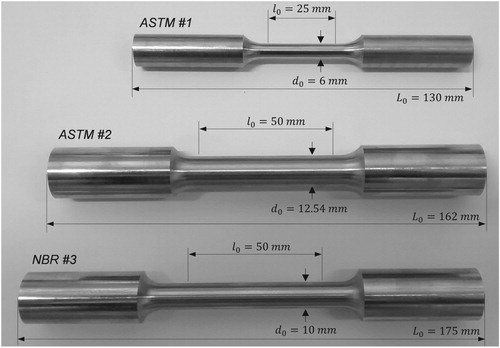
The proposed methodology is applied to the identification of hardening parameters of the AISI 304 stainless steel based on tensile tests with specimens of three different geometries and prepared according to the American ASTM E 8M [30] and Brazilian ABNT NBR ISO 6892 [31] standards. The tensile tests were performed with controlled displacements with crosshead velocity $v_c=3$ mm/min at room temperature. Extensometers with initial gauge length $l_0=25$ mm and $l_0=50$ mm were used according to the specimen size. Experimental loading is associated with elongations, also known as engineering strains, $e=\mathrm{\Delta }l/l_0$, where $\mathrm{\Delta }l$ represents the variation of the gauge length for a given tensile load. Figure 1 shows the actual specimens and main dimensions. The specimens are referred in this work as follows:

• ASTM #1: initial diameter $d_0=6.0$ mm and gauge length $l_0=25$ mm;

• ASTM #2: initial diameter $d_0=12.54$ mm and gauge length $l_0=50$ mm;

• NBR #3: initial diameter $d_0=10.0$ mm and gauge length $l_0=50$ mm.

Figure 1. Specimens for the ASTM and ABNT-NBR standards.

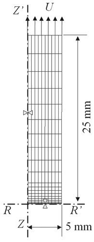
The geometrical model of all specimens accounts for symmetry around the rotation axis $Z-Z^{\prime }$ and about the $R-R^{\prime }$ axis. Structured finite element meshes with eight-noded elements are used in the simulations. The specimens are discretised with 200 elements and 661 nodes with progressive refinement towards the specimen $R-R^{\prime }$ axis, as illustrated in Figure 2 for specimen NBR #3. The focus of the work is the strategy to obtain the hardening parameters; therefore, typical values of the Young modulus and Poisson's ratio for austenitic steel AISI 304 were used in the simulations as E = 205 GPa and $\nu =0.29$, respectively. Notwithstanding, the value of the Young modulus was corroborated by curve-fitting true strains and stresses within the elastic envelope.

Figure 2. Finite element mesh for the NBR #3 specimen ($l_0=50$ mm and $d_0=10$ mm).

Hardening description: The AISI 304 is the most used austenitic stainless steel due to its combination of good formability and corrosion resistance. The high ductility of the type 304 stainless steel allows large plastic deformation before failure onset, favouring cold work processing [32], thereby making possible to manufacture with greater efficiency products and components, such as consumer items (cutlery, pans, sinks, etc.), architectural components (ornamental work, decorative panels, poolside fittings and fixings, etc.) and industrial equipment (e.g. pharmaceutical, food and beverage, chemical and mining equipment, etc.). Table 2 presents the chemical composition of the AISI 304 stainless steel used in this work.

Table 2. Chemical composition of the AISI 304 steel (in wt.%).

	Cr	Ni	Mn	Si	C	P	S
Nominal	18−20	8−10.5	$max2.0$	$max1.0$	$max0.08$	$max0.045$	$max0.03$
This work	18.677	8.780	1.9856	0.21897	0.07612	0.01984	0.02767

It is noteworthy that the AISI 304 stainless steel is characterized by deformation-induced phase transformation of austenite to martensite. Notwithstanding, De et al. [33] reported that stress–strain curves for temperatures higher than 298 K and low strain rates follow a typical ‘parabolic’ evolution, which makes possible to model inelastic deformation using phenomenological approaches.

The choice of the hardening equation within the framework of phenomenological models is essential to obtain the best possible approximation of the stress–strain paths of a deforming solid. El-Magd's [9] hardening equation (also known as modified Voce equation) is adopted in this work due to the good results reported for austenitic steels. El-Magd [9] derived a phenomenological hardening equation following the physical mechanisms of dislocation theory. The author assumes a Taylor-like correlation between the yield stress and total dislocation density in conjunction with Mecking and Kocks' [34] expression for the evolution of the dislocation density, allied to an improved description of the storage rate, so that (6) $\begin{array}{rl}{\sigma }_Y\left({\overline{\epsilon }}_p\right)& =C_1+C_2{\overline{\epsilon }}_p+C_3[1-\exp (-C_4{\overline{\epsilon }}_p)]\\ & ={\sigma }_0+\zeta {\overline{\epsilon }}_p+({\sigma }_{\mathrm{\infty }}-{\sigma }_0)[1-\exp (-\delta {\overline{\epsilon }}_p)],\end{array}$(6) in which $C_1={\sigma }_0$ is the initial yield stress, $C_2=\zeta$ is the linear hardening coefficient, $C_3={\sigma }_{\mathrm{\infty }}-{\sigma }_0$ is associated with the saturation stress, ${\sigma }_{\mathrm{\infty }}$, $C_4=\delta$ is the rate of approximation to linear hardening and ${\overline{\epsilon }}_p$ is the equivalent plastic strain. Noticeably, despite its micromechanical origin, Equation (6(6) $\begin{array}{rl}{\sigma }_Y\left({\overline{\epsilon }}_p\right)& =C_1+C_2{\overline{\epsilon }}_p+C_3[1-\exp (-C_4{\overline{\epsilon }}_p)]\\ & ={\sigma }_0+\zeta {\overline{\epsilon }}_p+({\sigma }_{\mathrm{\infty }}-{\sigma }_0)[1-\exp (-\delta {\overline{\epsilon }}_p)],\end{array}$(6) ) is phenomenological with hardening parameters, $\mathit{p}=[{\sigma }_0{\sigma }_{\mathrm{\infty }}\zeta \delta {]}^T$. In addition, the literature shows a large number of applications of Equation (6(6) $\begin{array}{rl}{\sigma }_Y\left({\overline{\epsilon }}_p\right)& =C_1+C_2{\overline{\epsilon }}_p+C_3[1-\exp (-C_4{\overline{\epsilon }}_p)]\\ & ={\sigma }_0+\zeta {\overline{\epsilon }}_p+({\sigma }_{\mathrm{\infty }}-{\sigma }_0)[1-\exp (-\delta {\overline{\epsilon }}_p)],\end{array}$(6) ) to different metal materials, ranging from Dual Phase (DP) and Transformation Induced Plasticity (TRIP) to high-alloyed carbon and stainless steels [9,35,36].

3.2. Stage 1: parameter identification of individual tests

The first stage of the identification strategy aims to find the best possible minimum for each individual tensile test, represented by the objective function, $g_s^{min}$. In this work, the number of inelastic parameters ($\mathit{p}=[{\sigma }_0{\sigma }_{\mathrm{\infty }}\zeta \delta {]}^T$) and mechanical tests (ASTM #1, ASTM #2, NBR #3) are $n_p=4$ and $n_s=3$, respectively. The values of the minimum fitness, $g_s^{min}$, are determined by individual solutions for each tensile test/specimen using the optimization problem established in Equation (1(1) $\begin{array}{lll}\text{Minimize}& {\displaystyle g_s(\mathit{p})}& \mathit{p}\in R^{n_p}\\ \text{Such that}& p_i^{\inf }\le p_i\le p_i^{\sup }& i=1,\dots ,n_p\end{array}$(1) ). For the sake of objectivity, the assessment of the capacity of the NM algorithm to solve individual problems of inelastic parameter identification is omitted here and the reader is referred to Vaz Jr. et al. [27].

Table 3 presents the hardening parameters of El-Magd's equation obtained by solving the optimization problem for each tensile test separately. Since the optimization procedure is performed individually, different sets of hardening parameters have been determined for specimens ASTM #1, ASTM #2 and NBR #3, i.e. ${\mathit{P}}^{min}=[{\mathit{p}}_1^{min}{\mathit{p}}_2^{min}{\mathit{p}}_3^{min}{]}^T$. Notwithstanding, the important results at this stage are the values of the best individual fitness, ${\mathit{G}}^{min}=[g_1^{min}{g}_2^{min}{g}_3^{min}{]}^T$.

Table 3. Identification of material parameters, ${\mathit{p}}_s^{min}$, and minimum individual fitness, $g_s^{min}$ for each individual tensile test.

Test ‘s’	Tensile test	${\sigma }_0$ [MPa]	${\sigma }_{\mathrm{\infty }}$ [MPa]	ζ [MPa]	δ	$g_s^{min}\times {10}^3$
1	ASTM #1	405.89	839.36	714.47	5.3900	7.2273
2	ASTM #2	421.45	991.70	372.92	4.6021	7.9852
3	NBR #3	409.16	878.59	597.24	5.1941	7.9447

Figure 3 presents the load × elongation curves for all three specimens evaluated using the material parameters indicated in Table 3. For instance, the thin solid lines depicted in Figure 3 represent load evolution computed using the hardening parameters determined for specimen ASTM #2 (${\sigma }_0=421.45$ MPa, ${\sigma }_{\mathrm{\infty }}=991.70$ MPa, $\zeta =372.92$ MPa and $\delta =4.6021$). Therefore, the numerical and experimental load curves for specimen ASTM #2 show a very close approximation and differences are visually imperceptible. However, simulations using this set of parameters for specimens ASTM #1 and NBR #3 present somewhat poorer results after the maximum load (in this case load predictions are grossly underestimated). Similar behaviour is observed for hardening parameters obtained for specimens ASTM #1 (thick solid lines) and NBR #3 (dashed lines). It is interesting to mention that differences in the general behaviour of the load evolution observed in Figure 3 are due to the phenomenological character of the constitutive model used in the simulations.

Figure 3. Load evolution for specimens ASTM #1, ASTM #2 and NBR #3 computed using parameters determined individually.

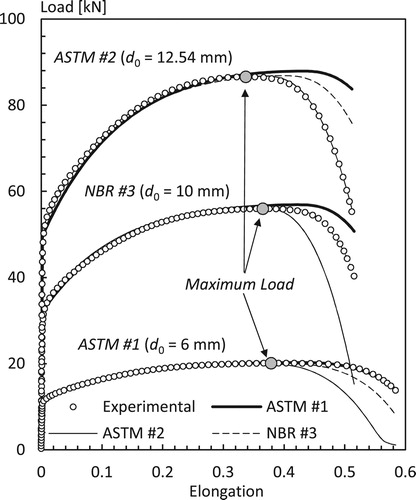
Remark 3.1

Despite widespread practice in industry, Figure 3 clearly shows that hardening parameters determined using a single tensile test/specimen is subject to inaccuracies after maximum load. The differences may reach unacceptable levels, such as the results obtained using material parameters determined for specimen ASTM #2.

3.3. Stage 2: parameter identification of simultaneous tests

The results discussed in the previous section indicate that parameter identification based on a single test is subject to inaccuracies for large plastic deformations under triaxial stress states (after maximum load). Therefore, the proposed methodology aims to obtain a better representative set of parameters for the AISI 304 steel by including additional information to the identification technique (i.e. by taking into account simultaneous tensile tests).

The general principle is the following: the best set of material parameters, $\mathit{p}$, must yield the minimum differences between $g_1(\mathit{p})$ and $g_1^{min}$, $g_2(\mathit{p})$ and $g_2^{min}$, and $g_3(\mathit{p})$ and $g_3^{min}$ for tensile tests ASTM #1, ASTM #2 and NBR #3, respectively.

The composed objective function: The optimization problem described by Equation (3(3) $\begin{array}{lll}\text{Minimize}& {\displaystyle g(\mathit{p},\mathit{\lambda })=\sum _{s=1}^{n_s}{\lambda }_s{g}_s(\mathit{p})}& \mathit{p}\in R^{n_p}\\ \text{Such that}& p_i^{\inf }\le p_i\le p_i^{\sup }& i=1,\dots ,n_p\end{array}$(3) ) finds the material parameters, $\mathit{p}$, accounting for the composed fitness, $g(\mathit{p},\mathit{\lambda })={\lambda }_1{g}_1(\mathit{p})+{\lambda }_2{g}_2(\mathit{p})+{\lambda }_3{g}_3(\mathit{p})$. Thus the solution of this problem for a given set of weights, $\mathit{\lambda }$, provides also the individual fitness $g_1(\mathit{p})$, $g_2(\mathit{p})$ and $g_3(\mathit{p})$. Table 4 presents the limiting cases, referred to as Cases (A), (B) and (C).

Table 4. Individual, $g_s(\mathit{p})$, and global, $G(\mathit{\lambda })$, fitness measures for Cases (A), (B) and (C).

		Weights			ASTM#1	ASTM#2	NBR#3
Case	${\lambda }_1$	${\lambda }_2$	${\lambda }_3$	$g(\mathit{p},\mathit{\lambda })\times {10}^3$	$g_1\times {10}^3$	$g_2\times {10}^3$	$g_3\times {10}^3$	$G(\mathit{\lambda })$
(A) – ASTM#1	1	0	0	7.2273	7.2273	141.1158	59.5913	10.3315
(B) – ASTM#2	0	1	0	7.9852	297.7274	7.9852	158.8650	25.6675
(C) – NBR#3	0	0	1	7.9447	106.1674	101.7141	7.9447	10.4112

Note: Best possible minimum: $g_1^{min}=7.2273\times {10}^{-3}$, $g_2^{min}=7.9852\times {10}^{-3}$ and $g_3^{min}=7.9447\times {10}^{-3}$.

For Case (A), the weight set is ${\mathit{\lambda }}^{(A)}=\{{\lambda }_1^{(A)}=1,{\lambda }_2^{(A)}=0,{\lambda }_3^{(A)}=0\}$, leading to parameter identification based solely on specimen ASTM #1. In this case, for the optimization problem defined in Equation (3(3) $\begin{array}{lll}\text{Minimize}& {\displaystyle g(\mathit{p},\mathit{\lambda })=\sum _{s=1}^{n_s}{\lambda }_s{g}_s(\mathit{p})}& \mathit{p}\in R^{n_p}\\ \text{Such that}& p_i^{\inf }\le p_i\le p_i^{\sup }& i=1,\dots ,n_p\end{array}$(3) ), the composed fitness is $g({\mathit{p}}^{(A)},{\mathit{\lambda }}^{(A)})=g_1({\mathit{p}}^{(A)})=7.2273\times {10}^{-3}$ (the hardening parameters are presented in Table 3 and the solid thick lines are depicted in Figure 3). Contrastingly, the individual fitness for specimens ASTM #2 and NBR #3 using the same material set are substantially larger, i.e. $g_2({\mathit{p}}^{(A)})=141.1158\times {10}^{-3}$ and $g_3({\mathit{p}}^{(A)})=59.5913\times {10}^{-3}$. Similar conclusion can be drawn for Cases (B) and (C) when the material parameters are obtained using specimens ASTM #2 and NBR #3, respectively.

At this stage, one can pose the following question: how can be established the best set of parameters, $\mathit{p}$, for all mechanical tests? This work introduces the mean global error $G(\mathit{\lambda })$, defined in Equation (5(5) $G(\mathit{\lambda })\equiv G[g_s(\mathit{p},{\lambda }_s)]=\sqrt{\frac{1}{n_s}\sum _{s=1}^{n_s}{\left[\frac{g_s^{min}-g_s(\mathit{p},{\lambda }_s)}{g_s^{min}}\right]}^2},$(5) ), which represents a quadratic relative difference between the best possible minimum, $g_s^{min}$, and the individual fitness $g_s(\mathit{p})$ obtained for a given set of weights $\mathit{\lambda }$. Table 4 also shows the mean global fitness, $G(\mathit{\lambda })$, for Cases (A)−(C). Noticeably, the worst set corresponds to Case (B), $G(\mathit{\lambda })=25.6675$, which can be clearly observed in Figure 3 for the curves portrayed by the thin solid lines (ASTM #2).

Remark 3.2

It is interesting to note that the best fit for individual specimens ASTM #1, ASTM #2 and NBR #3 does not guarantee small mean global errors $G(\mathit{\lambda })$. Therefore, the next question comes naturally: what are the weights, ${\lambda }_s$, which yield the best average approximation to the experimental data for all tests, i.e. the smallest mean global error, $G(\mathit{\lambda })$? The answer is given by the solution of the optimization problem established in Equation (4(4) $\begin{array}{lcl}\text{Minimize}& {\displaystyle G(\mathit{\lambda })}& \mathit{\lambda }\in R^{n_s}\\ \text{Such that}& {\displaystyle 0\le {\lambda }_s\le 1}& s=1,\dots ,n_s\\ & {\displaystyle \sum _{s=1}^{n_s}{\lambda }_s=1}& \end{array}$(4) ).

Finding the best set of weights ${\lambda }_s$: The global optimization problem is defined in Equation (4(4) $\begin{array}{lcl}\text{Minimize}& {\displaystyle G(\mathit{\lambda })}& \mathit{\lambda }\in R^{n_s}\\ \text{Such that}& {\displaystyle 0\le {\lambda }_s\le 1}& s=1,\dots ,n_s\\ & {\displaystyle \sum _{s=1}^{n_s}{\lambda }_s=1}& \end{array}$(4) ) and consists of finding the set of weights that provides the smallest mean global error $G(\mathit{\lambda })$. It is noteworthy that this problem differs from those previously described by using the weights, ${\lambda }_s$, as design variables instead of material parameters. Owing to the novelty of the concept, a brief discussion on the optimization progress is presented.

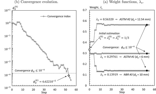
The Nelder–Mead algorithm is also adopted for this problem with design variables $\mathit{\lambda }=[{\lambda }_1{\lambda }_2{\lambda }_3{]}^T$, such that $0⩽{\lambda }_s⩽1$, $\sum _{s=1}^{n_s}{\lambda }_s=1$, and $n_s=3$. The initial estimate used in this example is ${\lambda }_1^{(0)}={\lambda }_2^{(0)}={\lambda }_3^{(0)}=1/3$. As the optimization process advances, the Nelder–Mead polytope moves towards the minimum and decreases in size. Therefore, the mean relative distance between the centrepoint and all vertices of the polytope is used as convergence measure, (7) ${\varphi }_d^{(k)}=\frac{\overline{d}({\mathit{\lambda }}^{(k)})}{\overline{d}({\mathit{\lambda }}^{(0)})},\mathrm{where}\overline{d}({\mathit{\lambda }}^{(k)})=\frac{1}{n_s+1}\sum _{j=1}^{n_s+1}\sqrt{\sum _{s=1}^{n_s}{({\lambda }_{j,s}^{(k)}-{\overline{\lambda }}_s^{(k)})}^2},$(7) in which $(k)$ indicates the iterative step, ${\overline{\lambda }}_s^{(k)}=1/(n_s+1)\sum _{i=1}^{n_s+1}{\lambda }_{s,i}^{(k)}$ is the coordinate of the centrepoint in the direction $s=1,\dots ,n_s$, and $n_s+1$ is the number of vertices of the polytope. In this work, convergence is assumed when the initial polytope reduces more than 10,000 times its initial size, i.e. $TO{L}_d⩽{10}^{-4}$.

The capacity of the algorithm to achieve convergence is illustrated in Figure 4(a), which shows a steady decrease of the relative size of the polytope as the optimization process advances. Evolution of the weights, ${\lambda }_s$, as the optimization progresses is presented in Figure 4(b). It is observed that ${\lambda }_s$ reaches the final level early in the iterative process, with some fine tuning towards the convergence.

Figure 4. Convergence evolution for the global optimization problem for weights ${\lambda }_1$, ${\lambda }_2$ and ${\lambda }_3$: (a) weight functions, ${\lambda }_s$ and (b) convergence evolution.

The final hardening parameters: The final hardening parameters are those which minimizes the global fitness, $G(\mathit{\lambda })$, providing a set of material parameters, $\mathit{p}$, that prompts the smallest relative differences between the experimental data and computed tensile loads for all mechanical tests.

The final material parameters and weights are presented in Table 5. The large differences between values of ${\lambda }_1$, ${\lambda }_2$ and ${\lambda }_3$ at final convergence indicate different effects that each tensile test imposes upon the final values of the material parameters. In this work, the largest value of ${\lambda }_2$ shows that the tensile test of specimen ASTM #2 plays the most important role in finding the representative set of hardening parameters for all mechanical tests. Despite the fact that the highest tensile loads are associated with specimen ASTM #2 ($d_0=12.54$ mm), one cannot directly correlate load levels and weight values, ${\lambda }_s$. It is observed that the second highest tensile loads are required by specimen NBR #3 ($d_0=10$ mm) and yet it presents the smallest weight, ${\lambda }_3=0.13919$.

Table 5. Final material parameters, $\mathit{p}$, weights, $\mathit{\lambda }$, and mean global fitness, $G(\mathit{\lambda })$.

	Symbol	Value
Material parameters	${\sigma }_0$	402.28 MPa
	${\sigma }_{\mathrm{\infty }}$	663.21 MPa
	ζ	887.95 MPa
	δ	11.3204
Weights	${\lambda }_1^{min}$ (ASTM #1)	0.29761
	${\lambda }_2^{min}$ (ASTM #2)	0.56320
	${\lambda }_3^{min}$ (NBR #3)	0.13919
Fitness	$G({\mathit{\lambda }}^{min})$	7.9210

The results indicate that the initial yield stress, ${\sigma }_0$, is predicted with acceptable accuracy either using single tensile tests (Table 3) or the multi-test approach (Table 5), with average differences around 2.5 %. However, the relative variations of the other parameters are significantly larger, reaching values as high as 36.2 %, 36.8 % and 55.3 % for ${\sigma }_{\mathrm{\infty }}$, ζ and δ, respectively. The discrepancies in the values of the material parameters for the limiting cases are reflected by the global fitness, which are 30.43 %, 224.04 % and 31.44 % larger than the $G({\mathit{\lambda }}^{min})$ obtained by the multi-test strategy, i.e. by comparing $G(\mathit{\lambda })$ shown in Table 4 for Cases (A), (B) and (C) against the global fitness, $G({\mathit{\lambda }}^{min})$, obtained by the proposed technique and presented in Table 5.

Figure 5 shows the load–elongation curves for specimens ASTM #1, ASTM #2 and NBR #3 computed using parameters obtained by the proposed optimization strategy (Table 5). The behaviour of the computed loading curves expresses the requirement established by the objective function defined in Equation (2(2) $g_s\left(\mathit{p}\right)=\sqrt{\frac{1}{N_s}\sum _{j=1}^{N_s}{\left(\frac{R_{s,j}^{Exp}-R{\left(\mathit{p}\right)}_{s,j}^{Num}}{R_{s,j}^{Exp}}\right)}^2},$(2) ), i.e. minimization of the relative quadratic errors prompts larger absolute differences for higher tensile loads. Therefore, one can observe in Figure 5 that specimen ASTM #2 presents the largest absolute differences, followed by specimens NBR #3 and ASTM #1, with corresponding maximum experimental loads 86.61 kN ($d_0=12.54$ mm), 55.97 kN ($d_0=10$ mm) and 20.12 kN ($d_0=6$ mm).

Figure 5. Load evolution for specimens ASTM #1, ASTM #2 and NBR #3 computed using parameters determined by the multi-test optimization scheme.

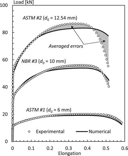
Remark 3.3

The differences between the experimental and numerical loading curves observed in Figure 5 reflects the nature of all yield stress equations based on phenomenological approaches. In spite of the good representation of the load-elongation curve when using a single specimen, the lack of micromechanical information gives rise to differences when multiple mechanical tests are used. It is important to mention that these remarks are not restricted to austenitic stainless steels.

4. Concluding remarks

The good formability characteristics of the AISI 304 stainless steel have led to a growing number of applications ranging from industrial equipment, architectural components and other consumer items. Therefore, the numerical simulation of forming operations has a great potential to help reducing manufacturing costs and improving forming efficiency. In such case, knowledge of representative values of the hardening parameters is essential. This study is inserted within this framework which introduces a new strategy to determine inelastic parameters based on multiple tensile tests.

The proposed multi-test identification technique can also be used in conjunction with different mechanical tests (e.g. biaxial, pin-on-disc and punch tests) and/or under specific testing conditions (e.g. temperature and strain-rate sensitivity) in order determine a particular material parameter or to capture the interrelation of parameters associated with other phenomena. In the present case, only isothermal tensile tests were utilized in order to isolate the isotropic strain hardening phenomena from other effects. It is important to note that, in case of different types of experiment, each test has its own experimental curve and target individual fitness $g_s^{min}$, so that the optimization of the global objective function, Equations (4(4) $\begin{array}{lcl}\text{Minimize}& {\displaystyle G(\mathit{\lambda })}& \mathit{\lambda }\in R^{n_s}\\ \text{Such that}& {\displaystyle 0\le {\lambda }_s\le 1}& s=1,\dots ,n_s\\ & {\displaystyle \sum _{s=1}^{n_s}{\lambda }_s=1}& \end{array}$(4) )–(5(5) $G(\mathit{\lambda })\equiv G[g_s(\mathit{p},{\lambda }_s)]=\sqrt{\frac{1}{n_s}\sum _{s=1}^{n_s}{\left[\frac{g_s^{min}-g_s(\mathit{p},{\lambda }_s)}{g_s^{min}}\right]}^2},$(5) ), makes possible to obtain the set of parameters which best fit for all types of experiments simultaneously.

In this work, the specimens were prepared according to the American ASTM E 8M [30] and Brazilian ABNT NBR ISO 6892 [31] standards. The tensile tests were carried out up to macroscopic failure aiming at determining inelastic parameters associated with large plastic strains. The study shows that hardening parameters obtained using a single tensile test is subject to some variability for large plastic deformations. For instance, parameter identification based solely on specimen ASTM #2 provided material parameters which led to substantial premature load reduction for specimens ASTM #1 and NBR #3.

A combination between the objective function computed for all mechanical tests associated with a global fitness was able to determine a representative set of material parameters for the AISI 304 stainless steel. The simulations indicated significant reduction of the global error when comparing against single test results. Some differences were observed for the final set of hardening parameters due to the phenomenological modelling approach. Notwithstanding, it is noteworthy that phenomenological models have largely been used in industry owing to availability in commercial software.

Disclosure statement

No potential conflict of interest was reported by the author(s).

ORCID

M. Vaz Jr. http://orcid.org/0000-0001-6202-8592

M. Tomiyama http://orcid.org/0000-0002-9234-6425

Additional information

Funding

The authors acknowledge the financial support provided by the Brazilian funding agency Conselho Nacional de Desenvolvimento Científico e Tecnológico (CNPq) (National Council for Scientific and Technological Development), Grant no. 303412/2016-0.

Appendix

Mechanical incremental boundary value problem

Identification of inelastic parameters based on optimization schemes requires the solution of a direct mechanical incremental boundary value problem. Therefore, the robustness of the inverse problem is directly dependent upon a robust elastic–plastic formulation and corresponding discretization method, i.e. the mathematical/numerical model must account for finite strains and properly handle the associate kinematics. Moreover, the iterative scheme must provide quadratic rate of convergence since the optimization method requires multiple runs of the code.

Plasticity approach: The present plasticity formulation is based upon thermodynamics of irreversible processes and uses the equivalent plastic strain, ${\overline{\epsilon }}_p$, as internal variable (which directly affects the yield stress, Equation (6(6) $\begin{array}{rl}{\sigma }_Y\left({\overline{\epsilon }}_p\right)& =C_1+C_2{\overline{\epsilon }}_p+C_3[1-\exp (-C_4{\overline{\epsilon }}_p)]\\ & ={\sigma }_0+\zeta {\overline{\epsilon }}_p+({\sigma }_{\mathrm{\infty }}-{\sigma }_0)[1-\exp (-\delta {\overline{\epsilon }}_p)],\end{array}$(6) )) associated with the classical von Mises constitutive model. Associate flow and hardening rules in conjunction with a strain-hardening approach were adopted in plasticity model. The stress integration uses a predictor–corrector stress update algorithm.

It is important to mention that the plasticity model is essentially phenomenological, which provides an empirical description of the phenomena that is consistent with the underlying theory, but not directly derived from its principles (e.g. the model does not account for directly mechanisms of dislocation theory). For the sake of objectivity, the reader is referred to Lubliner [37] and Souza Neto et al. [38] for further details.

Incremental boundary value problem: The mechanical boundary value problem is characterized by the equilibrium equations, which are expressed by linear and angular momentum conservation laws, respectively defined as (A1) $\begin{array}{l}{\displaystyle \mathrm{div}[\mathit{\sigma }]+\rho \mathit{b}=0}\\ {\displaystyle \mathit{\sigma }={\mathit{\sigma }}^T}\end{array}\mathrm{with}\begin{array}{l}\mathit{u}={\mathit{u}}^a\mathrm{for}\mathit{x}\in \mathrm{\partial }{\mathrm{\Omega }}^u\\ \mathit{\sigma }\mathit{n}={\mathit{t}}^a\mathrm{for}\mathit{x}\in \mathrm{\partial }{\mathrm{\Omega }}^t\end{array}\mathrm{and}\begin{array}{l}\mathrm{\partial }\mathrm{\Omega }=\mathrm{\partial }{\mathrm{\Omega }}^u\cup \mathrm{\partial }{\mathrm{\Omega }}^t\\ \mathrm{\partial }{\mathrm{\Omega }}^u\cap \mathrm{\partial }{\mathrm{\Omega }}^t=\varnothing \end{array}$(A1) where $\mathit{\sigma }$ is the Cauchy stress tensor, $\mathit{b}$ is the body force per unit mass, $\mathit{u}$ are displacements, ρ is the specific mass, and $\mathit{n}$ is the outward normal unit vector. The boundary conditions are generally described by applied displacements and loads, ${\mathit{u}}^a$ and ${\mathit{t}}^a$, respectively.

The finite element method based on an update Lagrangian approach is used to solve Equation (A1(A1) $\begin{array}{l}{\displaystyle \mathrm{div}[\mathit{\sigma }]+\rho \mathit{b}=0}\\ {\displaystyle \mathit{\sigma }={\mathit{\sigma }}^T}\end{array}\mathrm{with}\begin{array}{l}\mathit{u}={\mathit{u}}^a\mathrm{for}\mathit{x}\in \mathrm{\partial }{\mathrm{\Omega }}^u\\ \mathit{\sigma }\mathit{n}={\mathit{t}}^a\mathrm{for}\mathit{x}\in \mathrm{\partial }{\mathrm{\Omega }}^t\end{array}\mathrm{and}\begin{array}{l}\mathrm{\partial }\mathrm{\Omega }=\mathrm{\partial }{\mathrm{\Omega }}^u\cup \mathrm{\partial }{\mathrm{\Omega }}^t\\ \mathrm{\partial }{\mathrm{\Omega }}^u\cap \mathrm{\partial }{\mathrm{\Omega }}^t=\varnothing \end{array}$(A1) ). The elastic–plastic problem uses a hyperelastic formulation combined with a multiplicative decomposition of the deformation gradient into elastic and plastic components, $\mathit{F}={\mathit{F}}^e{\mathit{F}}^p$. The incremental boundary value problem is defined by means of the principle of the virtual power, so that (A2) ${\int }_{{\mathrm{\Omega }}_{n+1}}[\hat{\mathit{\sigma }}({\mathit{\alpha }}_n,\mathit{F}({\mathit{u}}_{n+1})):\delta \mathit{d}]\mathrm{d}v-{\int }_{{\mathrm{\Omega }}_{n+1}}(\rho \mathit{b}{)}_{n+1}\cdot \delta \mathit{\eta }\mathrm{d}v-{\int }_{\mathrm{\partial }{\mathrm{\Omega }}_{n+1}}{\mathit{t}}_{n+1}\cdot \delta \mathit{\eta }\mathrm{d}a=0,$(A2) in which $\hat{\mathit{\sigma }}$ is the incremental constitutive function, ${\mathit{u}}_{n+1}$ and $\mathit{F}$ are the global displacement vector and deformation gradient at the end of interval $[t,t_{n+1}]$, ${\mathit{\alpha }}_n$ is a set of internal variables assumed constant in the same interval, $(\rho \mathit{b}{)}_{n+1}$ and ${\mathit{t}}_{n+1}$ are body forces and traction fields prescribed at time increment $t_{n+1}$, $\delta \mathit{\eta }$ is a kinematically admissible velocity field and $\delta \mathit{d}=\mathrm{Sym}[{\mathrm{\nabla }}_x(\delta \mathit{\eta })]$ is the corresponding rate of deformation tensor.

Discretization of Equation (A2(A2) ${\int }_{{\mathrm{\Omega }}_{n+1}}[\hat{\mathit{\sigma }}({\mathit{\alpha }}_n,\mathit{F}({\mathit{u}}_{n+1})):\delta \mathit{d}]\mathrm{d}v-{\int }_{{\mathrm{\Omega }}_{n+1}}(\rho \mathit{b}{)}_{n+1}\cdot \delta \mathit{\eta }\mathrm{d}v-{\int }_{\mathrm{\partial }{\mathrm{\Omega }}_{n+1}}{\mathit{t}}_{n+1}\cdot \delta \mathit{\eta }\mathrm{d}a=0,$(A2) ) follows the standard finite element procedure and consists of finding a kinematically admissible global displacements, ${\mathit{u}}_{n+1}$, which satisfies the incremental equilibrium equation: (A3) $\mathit{r}\left({\mathit{u}}_{n+1}\right)={\mathit{f}}^{Int}\left({\mathit{u}}_{n+1}\right)-{\mathit{f}}_{n+1}^{Ext},$(A3) where $\mathit{r}$ is the residual of the nonlinear problem at time step n + 1, and ${\mathit{f}}_{n+1}^{Int}$ and ${\mathit{f}}_{n+1}^{Ext}$ are the internal and external global force vectors, respectively, (A4) $\begin{array}{rl}{\displaystyle {\mathit{f}}_{n+1}^{int}}& ={\int }_{{\mathrm{\Omega }}_{n+1}}{\mathit{B}}_{n+1}^T\hat{\mathit{\sigma }}({\mathit{\alpha }}_n,\mathit{F}({\mathit{u}}_{n+1}))\mathrm{d}v,\\ {\displaystyle {\mathit{f}}_{n+1}^{ext}}& ={\int }_{{\mathrm{\Omega }}_{n+1}}{\mathit{N}}_{n+1}^T(\rho \mathit{b}{)}_{n+1}\mathrm{d}v+{\int }_{\mathrm{\partial }{\mathrm{\Omega }}_{n+1}}{\mathit{N}}_{n+1}^T{\mathit{t}}_{n+1}\mathrm{d}a,\end{array}$(A4) where the $\mathit{B}$-matrix is the discrete symmetric gradient operator with respect to the final configuration ${\mathit{x}}_{n+1}={\mathit{x}}_n+{\mathit{u}}_{n+1}$. The solution of the material and geometrically nonlinear problem is achieved by using the Newton–Raphson iterative algorithm via linearization of Equation (A3(A3) $\mathit{r}\left({\mathit{u}}_{n+1}\right)={\mathit{f}}^{Int}\left({\mathit{u}}_{n+1}\right)-{\mathit{f}}_{n+1}^{Ext},$(A3) ), as (A5) $\mathit{r}({\mathit{u}}_{n+1}^{(k)}+\delta {\mathit{u}}_{n+1}^{(k+1)})\cong \mathit{r}\left({\mathit{u}}_{n+1}^{(k)}\right)+\left[\frac{\mathrm{\partial }\mathit{r}\left({\mathit{u}}_{n+1}^{(k)}\right)}{\mathrm{\partial }{\mathit{u}}_{n+1}^{(k)}}\right]\delta {\mathit{u}}_{n+1}^{(k+1)},$(A5) so that (A6) ${\mathit{K}}_T\left({\mathit{u}}_{n+1}^{(k)}\right)\left[\delta {\mathit{u}}_{n+1}^{(k)}\right]=-\mathit{r}\left({\mathit{u}}_{n+1}^{(k)}\right)\text{and}{\mathit{u}}_{n+1}^{(k+1)}={\mathit{u}}_{n+1}^{(k)}+\delta {\mathit{u}}_{n+1}^{(k+1)},$(A6) in which ${\mathit{K}}_T=[\mathrm{\partial }{\mathit{r}}_{n+1}^{(k)}/\mathrm{\partial }{\mathit{u}}_{n+1}^{(k)}]$ is the tangent stiffness and $(k)$ indicates the Newton–Raphson iteration step. Further details on the finite element approximation are presented in Souza Neto et al. [38].

Noticeably, solution of Equations (A2(A2) ${\int }_{{\mathrm{\Omega }}_{n+1}}[\hat{\mathit{\sigma }}({\mathit{\alpha }}_n,\mathit{F}({\mathit{u}}_{n+1})):\delta \mathit{d}]\mathrm{d}v-{\int }_{{\mathrm{\Omega }}_{n+1}}(\rho \mathit{b}{)}_{n+1}\cdot \delta \mathit{\eta }\mathrm{d}v-{\int }_{\mathrm{\partial }{\mathrm{\Omega }}_{n+1}}{\mathit{t}}_{n+1}\cdot \delta \mathit{\eta }\mathrm{d}a=0,$(A2) )–(A6(A6) ${\mathit{K}}_T\left({\mathit{u}}_{n+1}^{(k)}\right)\left[\delta {\mathit{u}}_{n+1}^{(k)}\right]=-\mathit{r}\left({\mathit{u}}_{n+1}^{(k)}\right)\text{and}{\mathit{u}}_{n+1}^{(k+1)}={\mathit{u}}_{n+1}^{(k)}+\delta {\mathit{u}}_{n+1}^{(k+1)},$(A6) ) for each mechanical test/specimen ‘s’ using the hardening parameters, p, enables computation of the numerical tensile load, $R(\mathit{p}{)}^{Num}$, which in turn is used to evaluate the corresponding individual objective function defined in Equation (2(2) $g_s\left(\mathit{p}\right)=\sqrt{\frac{1}{N_s}\sum _{j=1}^{N_s}{\left(\frac{R_{s,j}^{Exp}-R{\left(\mathit{p}\right)}_{s,j}^{Num}}{R_{s,j}^{Exp}}\right)}^2},$(2) ).

References

- Samuel KG, Rodriguez P. On power-law type relationships and the Ludwigson explanation for the stress–strain behaviour of AISI 316 stainless steel. J Mater Sci. 2005;40:5727–5731. doi:10.1007/s10853-005-1078-9.
- Samuel KG. Limitations of Hollomon and Ludwigson stress-strain relations in assessing the strain hardening parameters. J Phys D Appl Phys. 2006;39:203–212. doi:10.1088/0022-3727/39/1/030.
- Hollomon JH. Tensile deformation. Trans AIME. 1945;162:268–290.
- Swift BH. Plastic instability under plane stress. J Mech Phys Solids. 1952;1:1–18. doi:10.1016/0022-5096(52)90002-1.
- Ludwigson DC. Modified stress–strain relation for FCC metals and alloys. Metal Trans. 1971;2:2825–2828. doi:10.1007/BF02813258.
- Kashyap BP, Tangri K. On the Hall–Petch relationship and substructural evolution in type 316L stainless steel. Acta Metall Mater. 1995;43:3971–39811. doi:10.1016/0956-7151(95)00110-H.
- Hertelé S, De Waele W, Denys R. A generic stress–strain model for metallic materials with two-stage strain hardening behaviour. Int J Non-linear Mech. 2011;46:519–531. doi:10.1016/j.ijnonlinmec.2010.12.004.
- Ramberg W, Osgood WR. Description of stress–strain curves by three parameters. Washington: NACA; 1943. (Technical note; no. 902).
- El-Magd E. Modeling and simulation of mechanical behavior, In: Totten GE, Xie L, Funatani K, editors. Modeling and simulation of material selection and mechanical design. New York: Dekker; 2004. Chapter 4.
- Voce E. The relationship between stress and strain for homogeneous deformation. J Inst Metals. 1948;74:537–562.
- Harth T, Schwan S, Lehn J, et al. Identification of material parameters for constitutive models: statistical analysis and design of experiments. Int J Plasticity. 2004;20:1403–1440. doi:10.1016/j.ijplas.2003.11.001.
- Haghdadi N, Martin D, Hodgson P. Physically-based constitutive modelling of hot deformation behavior in a LDX 2101 duplex stainless steel. Mater Design. 2016;106:420–427. doi:10.1016/j.matdes.2016.05.118.
- Mahnken R. Theoretical numerical and identification aspects of a new model class for ductile damage. Int J Plasticity. 2002;18:801–831. doi:10.1016/S0749-6419(00)00105-4.
- Wang M, Wu J. Identification of plastic properties of metal materials using spherical indentation experiment and Bayesian model updating approach. Int J Mech Sci. 2019;151:733–745. doi:10.1016/j.ijmecsci.2018.12.027.
- Pacheco CC, Dulikravich GS, Vesenjak M, et al. Inverse parameter identification in solid mechanics using Bayesian statistics response surfaces and minimization. Tech Mech. 2016;36:120–131. doi:10.24352/ub.ovgu-2017-014.
- Vaz Jr. M, Muñoz-Rojas PA, Cardoso EL, et al. Considerations on parameter identification and material response for Gurson-type and Lemaitre-type constitutive models. Int J Mech Sci. 2016;106:254–265. doi:10.1016/j.ijmecsci.2015.12.014.
- Carniel TA, Muñoz-Rojas PA, Vaz Jr M. A viscoelastic viscoplastic constitutive model including mechanical degradation: uniaxial transient finite element formulation at finite strains and application to space truss structures. Appl Math Modelling. 2015;39:1725–1739. doi:10.1016/j.apm.2014.09.036.
- Jin YF, Yin ZY, Shen SL, et al. A new hybrid real-coded genetic algorithm and its application to parameters identification of soils. Inverse Probl Sci Eng. 2017;25:1343–1366. doi:10.1080/17415977.2016.1259315.
- Yoshida F, Urabe M, Hino R, et al. Inverse approach to identification of material parameters of cyclic elasto-plasticity for component layers of a bimetallic sheet. Int J Plasticity. 2003;19:2149–2170. doi:10.1016/S0749-6419(03)00063-9.
- Ponthot JP, Kleinermann JP. A cascade optimization methodology for automatic parameter identification and shape/process optimization in metal forming simulation. Comput Meth Appl Mech Eng. 2006;195:5472–5508. doi:10.1016/j.cma.2005.11.012.
- Vaz Jr. M, Hulse ER, Tomiyama M. A note on parameter identification of the AISI 304 stainless steel using micromechanical-based phenomenological approaches. Mater Res. 2019;22:e20190222. doi:10.1590/1980-5373-MR-2019-0222.
- Vaz Jr. M, Hulse ER, Tomiyama M. Identification of inelastic parameters of the AISI 304 stainless steel. In Öchsner A, Altenbach H, editors. Engineering design applications II. structures materials and processes. Chem: Springer Nature; 2020.
- Pierron F, Grédiac M. The virtual fields method: extracting constitutive mechanical parameters from full-field deformation measurements. New York: Springer; 2012.
- Martins JMP, Andrade-Campos A, Thuillier S. Comparison of inverse identification strategies for constitutive mechanical models using full-field measurements. Int J Mech Sci. 2018;145:330–345. doi: 10.1016/j.ijmecsci.2018.07.013
- Nelder JA, Mead R. A simplex method for function minimization. Comput J. 1965;7:308–313. doi:10.1093/comjnl/8.1.27. doi: 10.1093/comjnl/7.4.308
- Lagarias JC, Reeds JA, Wright MH, et al. Convergence properties of the Nelder–Mead simplex method in low dimensions. SIAM J Optim. 1998;9:112–147. doi:10.1137/S1052623496303470.
- Vaz Jr. M, Cardoso EL, Muñoz-Rojas PA, et al. Identification of constitutive parameters – optimization strategies and applications. Mat-wiss U Werkstofftech. 2015;46:447–491. doi:10.1002/mawe.201500423.
- Vaz Jr M, Cardoso EL, Stahlschmidt J. Particle swarm optimization and identification of inelastic material parameters. Eng Comput. 2013;30:936–960. doi:10.1108/EC-10-2011-0118.
- Vaz Jr. M, Luersen MA, Muñoz-Rojas PA, et al. Identification of inelastic parameters based on deep drawing forming operations using a global-local hybrid particle swarm approach. C R Mecanique. 2016;344:319–334. doi:10.1016/j.crme.2015.07.015.
- ASTM E8 / E8M-09. Standard test methods for tension testing of metallic materials. West Conshohocken: ASTM International; 2009.
- ABNT NBR ISO 6892. Metallic materials – tensile testing at ambient temperature. Rio de Janeiro: ABNT; 2002.
- Subramonian S, Kardes N. Materials for sheet forming. In: Altan T, Tekkaya E, editors. Sheet metal forming: fundamentals. Materials Park: ASM; 2012. p. 73–88.
- De AK, Speer JG, Matlock DK, et al. Deformation-induced phase transformation and strain hardening in yype 304 austenitic stainless steel. Metall Mater Trans A. 2006;36A:1875–1886. doi:10.1007/s11661-006-0130-y.
- Mecking H, Kocks UF. Kinetics of flow and strain hardening. Acta Metall. 1981;29:1865–1875. doi:10.1016/0001-6160(81)90112-7.
- Panich S, Barlat F, Uthaisangsuk V, et al. Experimental and theoretical formability analysis using strain and stress based forming limit diagram for advanced high strength steels. Mater Design. 2013;51:756–766. doi:10.1016/j.matdes.2013.04.080.
- Gruber M, Lebaal N, Roth S, et al. Parameter identification of hardening laws for bulk metal forming using experimental and numerical approach. Int J Mater Form. 2016;9:21–33. doi:10.1007/s12289-014-1196-5.
- Lubliner J. Plasticity theory. Mineola: Dover Publications; 2008.
- de Souza Neto EA, Peric D, Owen DRJ. Computational methods for plasticity: theory and applications. Chichester: Wiley; 2008.