Entropy binomial tree method and calibration for the volatility smile

Abstract

In this paper, we combine the maximum entropy principle with binomial tree to construct a non-recombining entropy binomial tree pricing model under the volatility that is a function of time, and give the rate of convergence. The model may yield an unbiased and objective probability. In addition, we research the calibration problem of volatility with the entropy binomial tree, and adopt an exterior penalty method to transform this problem into a nonlinear unconstrained optimization problem. For the optimization problem, we use the quasi-Newton algorithm. Finally, we test our model by numerical examples and options data on the S&P 500 index. The results confirm the effectiveness of the entropy binomial tree pricing model.

Keywords:

• Entropy binomial tree
• volatility
• option pricing
• calibration
• nonlinear constrained optimization

2010 Mathematics Subject Classifications:

• 91G20
• 91G60

1. Introduction

Options, as one of the most important and popular financial derivatives, encompass many other derivative securities through combination, which are used for both investing and hedging. The emergence of the Black–Scholes [1] model led to a boom in options trading because of its simplicity and clarity in obtaining the price of options. However, the closed-form solutions of continuous-time models may not be available, some numerical methods have been proposed to compute option prices and have received wide attention from both finance researchers and practitioners. So far there are some useful numerical methods, such as the Monte Carlo method [2], the tree method [3], and the finite difference method [4]. These discrete models provide an easy way to understand how uncertainties are resolved in a continuous-time asset pricing model.

The tree method is a popular method in option pricing because of its simplicity, efficiency and the ability to deal with the early exercise characteristic of the American options. The binomial tree method, as a discrete model proposed by Cox, Ross and Rubinstein (CRR) [3], is the most popular approach to pricing options. Because of the usefulness and importance of the binomial tree model, there are many researchers who investigate other trees [5–8]. The option prices computed by these models converge to the theoretical option value as the the number of time steps increases. However, there are some difficulties need to be overcome when applying this model to obtain the option price, such as the accuracy of solutions, the computational intensity and the determination of the model parameters p, u and d (with u, d representing the up and down factors, respectively, and p representing the risk-neutral probability ). When determining parameters u, d and p, we often need to impose some conditions, such as ud = 1. In addition, the probability p derived by the model is often negative or p>1. To overcome the traditional problems mentioned above, Li and Li [9] propose an entropy binomial tree model which provides a novel strategy to determine the parameters based on maximum entropy principle [10]. However, the constant volatility assumption cannot capture features of empirically observed option prices. In fact, the so-called volatility skew or smile phenomenon exists in all major stock index markets today.

Dupire [11] considers the local volatility model, where the volatility is a deterministic function of asset price and time, i.e. $\sigma =\sigma (S,t)$. The function of European call option $C(S,t)$ satisfies the following equation: (1) $\begin{array}{rl}& \frac{\mathrm{\partial }C}{\mathrm{\partial }t}+\frac{1}{2}{\sigma }^2(S,t)S^2\frac{{\mathrm{\partial }}^{2}C}{\mathrm{\partial }{S}^2}+rS\frac{\mathrm{\partial }C}{\mathrm{\partial }S}-rC=0,\\ & 0\le S<\mathrm{\infty },0\le t<T,\end{array}$(1) (2) $\begin{array}{rl}& C(S,T)=(S-K{)}^{+},0\le S<\mathrm{\infty }.\end{array}$(2) The boundary condition is $C(0,t)=0,\underset{S\to \mathrm{\infty }}{lim}C(S,t)-S=-K{e}^{-rt}.$ Dupire's equation is derived, which provides a very useful insight into the inverse problem of calibrating the local volatility model. In the case of $\sigma =\sigma (t)$, some efficient regularization methods have been developed for solving the corresponding inverse problem of estimating the volatility, see [12,13]. Moreover, in order to avoid the choice of regularization parameter and to obtain the error estimation of the reconstructed volatility, one can employ the inflection point method [14], which is originally developed for solving one dimensional integral equations. Inverse problem is usually ill-posed, which have been extensively studied [15–17].

A tree for a known local volatility surface is called local volatility tree, whereas an implied tree fits the implied volatility surface generated by a local volatility tree. The construction of the implied tree is thus an inverse problem, which in general is ill-posed [18]. Li [19] develops an implied binomial tree which sets the transition probabilities to some constant, negative probabilities will vanish. Derman et al. [20] propose an implied trinomial tree, but negative probabilities will appear. In order to eliminate the occurrences of negative transition probabilities, Barle and Cakici [21] improve the DKC (Derman, Kani and Chriss) model with a better placement of nodes. Crépey [22] calibrates the local volatility in a trinomial tree using Tikhonov regularization. Talias [23] calibrates the non-recombining tree by genetic algorithms. Charalambous et al. [24] construct an implied non-recombining tree and calibrate the volatility smile by quasi-Newton algorithm. Lok and Lyuu [25] find a potentially fundamental reason why the negative probabilities linger and construct a waterline tree for separable local volatility which combines two kinds of binomial trees by matching the moments of the underlying asset price and logarithmic asset price. Gong and Xu [26] propose an implied non-recombining trinomial tree and calibrate the volatility smile.

In this paper, we first propose a non-recombining binomial tree pricing model based on maximum entropy principle that the local volatility function only depends on time. We then give the convergence rates of the entropy binomial tree pricing model. In addition, we calibrate the volatility by using the entropy binomial tree. In particular, we attempt to minimize the least squares error between the market prices and the theoretical prices with respect to the underlying asset values at each node of the entropy binomial tree, subject to constraints of risk neutrality and no-arbitrage. Calibrating the volatility means that finding the stock prices and transition probabilities at each node of the tree, which makes the tree reproduce the option price that is consistent with today's market price. The calibration problem is a nonlinear optimization problem with constraints. Especially, we adopt a penalty method to transform the nonlinear optimization problem with constraints into a nonlinear unconstrained problem which is solved by quasi-Newton algorithm.

In contrast to other implied trees, our model overcomes the traditional classical problems mentioned above and does not employ node substitutions and set the transition probabilities to some constant. In addition, we do not need any interpolation or extrapolation across strikes and time in the process of calibration, and our model can be easily modified to account for options with different maturities. Finally, if needed, we can add smooth constraints to the distribution of the underlying asset for the extra degrees of freedom and the analytical structure of the model.

The paper is organized as follows. Brief introduction to binomial tree pricing model appears in Section 2. In Section 3, we consider the construction of binomial tree pricing model based on maximum entropy principle and give the convergence rate. In Section 4, we discuss the optimization algorithm and adopt a penalty method. For the optimization, we use a quasi-Newton algorithm. Numerical and empirical results are presented in Section 5. Conclusions are in Section 6.

2. CRR model

CRR model is introduced by Cox et al. [3]. It assumes the underlying asset price S follows Geometric Brownian motion, K is the strike price, r is the risk-free interest rate, the volatility σ is a constant, T is the maturity. $\mathrm{△}t=T/n$ is the time step. Let u and d denote the up and down factors by which the underlying asset price can move in the single time step $\mathrm{△}t$, where $u>1,0<d\le 1$ and ud = 1. Let p be the risk-neutral probabilities corresponding to the asset price increases. According to the moment information of the underlying asset, we have (3) $\begin{array}{rl}up+d(1-p)& =e^{r\mathrm{△}t},\\ u^{2}p+d^2(1-p)& =e^{(2r+{\sigma }^2)\mathrm{△}t},\\ ud& =1,\end{array}$(3) then we can get (4) $p=\frac{e^{r\mathrm{△}t}-d}{u-d},u=e^{\sigma \sqrt{\mathrm{△}t}},d=e^{-\sigma \sqrt{\mathrm{△}t}}.$(4) Due to the option values at the last time step are known, the option value at node $(i,j)$ is $\begin{array}{rl}C(i,j)& =e^{-r\mathrm{\Delta }t}[pC(i+1,j+1)+(1-p)C(i+1,j)],\\ i& =1,\dots ,n-1,j=1,\dots ,n-1.\end{array}$ where $C(i+1,j+1)$ and $C(i+1,j)$ denote the option values when the underlying asset price $S(i,j)$ increases to $S(i+1,j+1)$ and decreases to $S(i+1,j)$, respectively.

There are some deficiencies about this model. From this model, we can see that the imposed condition ud = 1 must be satisfied which lacks practically economic meaning, and the parameter p in (4(4) $p=\frac{e^{r\mathrm{△}t}-d}{u-d},u=e^{\sigma \sqrt{\mathrm{△}t}},d=e^{-\sigma \sqrt{\mathrm{△}t}}.$(4) ) may be negative or greater than 1. In addition, the model works only for constant volatility. Therefore, determining precise parameters for this model is very important. According to Equations (3(3) $\begin{array}{rl}up+d(1-p)& =e^{r\mathrm{△}t},\\ u^{2}p+d^2(1-p)& =e^{(2r+{\sigma }^2)\mathrm{△}t},\\ ud& =1,\end{array}$(3) ), we can see the model concerns moments of the underlying asset price and determines probability distribution of underlying asset price. From this insight, we propose a new strategy to determine parameters of the binomial tree that the volatility is a function of time based on maximum entropy principle.

3. Entropy optimization model of parameters

3.1. Entropy optimization model

The maximum entropy principle [10] states that ‘in making inference on the basis of partial information one must use that probability distribution which has maximum entropy subject to whatever is known. This is the only unbiased assignment one can make; to use any other amount to arbitrary assumption of information, which by hypothesis one does not have.’ Therefore we propose entropy binomial tree model when the volatility is a function of time.

Assume the underlying asset price S follows Geometric Brownian motion: $\mathrm{d}{S}_t=r{S}_t\mathrm{d}t+\sigma (t)S_t\mathrm{d}{W}_t,$ where r is the risk-free interest rate, the volatility σ is a deterministic function of time t, T is the maturity. Now, let's consider the binomial tree of underlying asset price, which stands as a discrete model of the Geometric Brownian motion [25]. Let i and j denote the time and underlying asset price dimension. $\mathrm{△}t=T/(n-1)$ is the time step, $S(i,j)$ is the value of the underlying asset at node $(i,j)$. Let $u(i,j)$ and $d(i,j)$ denote the up and down factors by which the underlying asset price can move in the single time step. Let $S(i+1,2j)$ and $S(i+1,2j-1)$ be the asset prices when the underlying asset price increases and decreases, respectively. Let $p(i,j)$ denote the upward risk-neutral probabilities. Then the entropy binomial tree optimization model is (5) $\begin{array}{rl}max& -p(i,j)\ln p(i,j)-(1-p(i,j))\ln (1-p(i,j))\\ \mathrm{s}.\mathrm{t}.& p(i,j)u(i,j)+(1-p(i,j))d(i,j)=e^{r\mathrm{△}t},\\ & p(i,j)u(i,j{)}^2+(1-p(i,j))d(i,j{)}^2=e^{2r\mathrm{△}t+{\sigma }_i^2\mathrm{△}t},\\ & 0\le p(i,j)\le 1,\\ & u(i,j)>1,\\ & 0<d(i,j)\le 1.\end{array}$(5) In the model, $p(i,j),u(i,j),d(i,j)$ are unknown quantities, and $r,{\sigma }_i,\mathrm{△}t$ are known quantities.

Remark 3.1

We will show that the solution to the entropy binomial tree optimization model (5(5) $\begin{array}{rl}max& -p(i,j)\ln p(i,j)-(1-p(i,j))\ln (1-p(i,j))\\ \mathrm{s}.\mathrm{t}.& p(i,j)u(i,j)+(1-p(i,j))d(i,j)=e^{r\mathrm{△}t},\\ & p(i,j)u(i,j{)}^2+(1-p(i,j))d(i,j{)}^2=e^{2r\mathrm{△}t+{\sigma }_i^2\mathrm{△}t},\\ & 0\le p(i,j)\le 1,\\ & u(i,j)>1,\\ & 0<d(i,j)\le 1.\end{array}$(5) ) does not depend on j.

3.2. Solving model

First, according to the first constraint of entropy binomial tree model (5(5) $\begin{array}{rl}max& -p(i,j)\ln p(i,j)-(1-p(i,j))\ln (1-p(i,j))\\ \mathrm{s}.\mathrm{t}.& p(i,j)u(i,j)+(1-p(i,j))d(i,j)=e^{r\mathrm{△}t},\\ & p(i,j)u(i,j{)}^2+(1-p(i,j))d(i,j{)}^2=e^{2r\mathrm{△}t+{\sigma }_i^2\mathrm{△}t},\\ & 0\le p(i,j)\le 1,\\ & u(i,j)>1,\\ & 0<d(i,j)\le 1.\end{array}$(5) ), we have $u(i,j)=\frac{e^{r\mathrm{△}t}-(1-p(i,j))d(i,j)}{p(i,j)}.$ Substituting $u(i,j)$ into second constraint, we get $d(i,j)=e^{r\mathrm{△}t}\pm \sqrt{\frac{p(i,j)}{1-p(i,j)}(e^{2r\mathrm{△}t+{\sigma }_i^2\mathrm{△}t}-e^{2r\mathrm{△}t})}.$ Hence $\begin{array}{rl}u(i,j)& =e^{r\mathrm{△}t}+\sqrt{\frac{1-p(i,j)}{p(i,j)}(e^{2r\mathrm{△}t+{\sigma }_i^2\mathrm{△}t}-e^{2r\mathrm{△}t})},\\ d(i,j)& =e^{r\mathrm{△}t}-\sqrt{\frac{p(i,j)}{1-p(i,j)}(e^{2r\mathrm{△}t+{\sigma }_i^2\mathrm{△}t}-e^{2r\mathrm{△}t})}.\end{array}$ or $\begin{array}{rl}u(i,j)& =e^{r\mathrm{△}t}-\sqrt{\frac{1-p(i,j)}{p(i,j)}(e^{2r\mathrm{△}t+{\sigma }_i^2\mathrm{△}t}-e^{2r\mathrm{△}t})},\\ d(i,j)& =e^{r\mathrm{△}t}+\sqrt{\frac{p(i,j)}{1-p(i,j)}(e^{2r\mathrm{△}t+{\sigma }_i^2\mathrm{△}t}-e^{2r\mathrm{△}t})}.\end{array}$ According to $0<d(i,j)\le 1$, $d(i,j)=e^{r\mathrm{△}t}+\sqrt{(p(i,j)/(1-p(i,j)))(e^{2r\mathrm{△}t+{\sigma }_i^2\mathrm{△}t}-e^{2r\mathrm{△}t})}>1$, we have (6) $\begin{array}{rl}u(i,j)& =e^{r\mathrm{△}t}+\sqrt{\frac{1-p(i,j)}{p(i,j)}(e^{2r\mathrm{△}t+{\sigma }_i^2\mathrm{△}t}-e^{2r\mathrm{△}t})},\\ d(i,j)& =e^{r\mathrm{△}t}-\sqrt{\frac{p(i,j)}{1-p(i,j)}(e^{2r\mathrm{△}t+{\sigma }_i^2\mathrm{△}t}-e^{2r\mathrm{△}t})}.\end{array}$(6) Then the optimization problem (5(5) $\begin{array}{rl}max& -p(i,j)\ln p(i,j)-(1-p(i,j))\ln (1-p(i,j))\\ \mathrm{s}.\mathrm{t}.& p(i,j)u(i,j)+(1-p(i,j))d(i,j)=e^{r\mathrm{△}t},\\ & p(i,j)u(i,j{)}^2+(1-p(i,j))d(i,j{)}^2=e^{2r\mathrm{△}t+{\sigma }_i^2\mathrm{△}t},\\ & 0\le p(i,j)\le 1,\\ & u(i,j)>1,\\ & 0<d(i,j)\le 1.\end{array}$(5) ) is transformed to: (7) $\begin{array}{rl}max& -p(i,j)\ln p(i,j)-(1-p(i,j))\ln (1-p(i,j))\\ \mathrm{s}.\mathrm{t}.& 0\le p(i,j)\le 1,\\ & e^{r\mathrm{△}t}+\sqrt{\frac{1-p(i,j)}{p(i,j)}(e^{2r\mathrm{△}t+{\sigma }_i^2\mathrm{△}t}-e^{2r\mathrm{△}t})}>1,\\ & 0<e^{r\mathrm{△}t}-\sqrt{\frac{p(i,j)}{1-p(i,j)}(e^{2r\mathrm{△}t+{\sigma }_i^2\mathrm{△}t}-e^{2r\mathrm{△}t})}\le 1.\end{array}$(7) The second constraint in Equation (7(7) $\begin{array}{rl}max& -p(i,j)\ln p(i,j)-(1-p(i,j))\ln (1-p(i,j))\\ \mathrm{s}.\mathrm{t}.& 0\le p(i,j)\le 1,\\ & e^{r\mathrm{△}t}+\sqrt{\frac{1-p(i,j)}{p(i,j)}(e^{2r\mathrm{△}t+{\sigma }_i^2\mathrm{△}t}-e^{2r\mathrm{△}t})}>1,\\ & 0<e^{r\mathrm{△}t}-\sqrt{\frac{p(i,j)}{1-p(i,j)}(e^{2r\mathrm{△}t+{\sigma }_i^2\mathrm{△}t}-e^{2r\mathrm{△}t})}\le 1.\end{array}$(7) ) is satisfied, and Problem (7(7) $\begin{array}{rl}max& -p(i,j)\ln p(i,j)-(1-p(i,j))\ln (1-p(i,j))\\ \mathrm{s}.\mathrm{t}.& 0\le p(i,j)\le 1,\\ & e^{r\mathrm{△}t}+\sqrt{\frac{1-p(i,j)}{p(i,j)}(e^{2r\mathrm{△}t+{\sigma }_i^2\mathrm{△}t}-e^{2r\mathrm{△}t})}>1,\\ & 0<e^{r\mathrm{△}t}-\sqrt{\frac{p(i,j)}{1-p(i,j)}(e^{2r\mathrm{△}t+{\sigma }_i^2\mathrm{△}t}-e^{2r\mathrm{△}t})}\le 1.\end{array}$(7) ) becomes (8) $\begin{array}{rl}max& -p(i,j)\ln p(i,j)-(1-p(i,j))\ln (1-p(i,j))\\ \mathrm{s}.\mathrm{t}.& \frac{{(e^{r\mathrm{△}t}-1)}^2}{e^{2r\mathrm{△}t+{\sigma }_i^2\mathrm{△}t}-2e^{r\mathrm{△}t}+1}\le p(i,j)<e^{-{\sigma }_i^2\mathrm{△}t}.\end{array}$(8)

Second, we know the solution of the following optimization problem (9) $\begin{array}{rl}max& -p\ln p-(1-p)\ln (1-p)\\ \mathrm{s}.\mathrm{t}.& 0\le p\le 1.\end{array}$(9)

According to optimization problem (9(9) $\begin{array}{rl}max& -p\ln p-(1-p)\ln (1-p)\\ \mathrm{s}.\mathrm{t}.& 0\le p\le 1.\end{array}$(9) ), the optimal solution of (5(5) $\begin{array}{rl}max& -p(i,j)\ln p(i,j)-(1-p(i,j))\ln (1-p(i,j))\\ \mathrm{s}.\mathrm{t}.& p(i,j)u(i,j)+(1-p(i,j))d(i,j)=e^{r\mathrm{△}t},\\ & p(i,j)u(i,j{)}^2+(1-p(i,j))d(i,j{)}^2=e^{2r\mathrm{△}t+{\sigma }_i^2\mathrm{△}t},\\ & 0\le p(i,j)\le 1,\\ & u(i,j)>1,\\ & 0<d(i,j)\le 1.\end{array}$(5) ) is given as follows:

Case 1. If $\frac{{(e^{r\mathrm{△}t}-1)}^2}{e^{2r\mathrm{△}t+{\sigma }_i^2\mathrm{△}t}-2e^{r\mathrm{△}t}+1}<e^{-{\sigma }_i^2\mathrm{△}t}<\frac{1}{2},$ the optimal solution is $p(i,j)=e^{-{\sigma }_i^2\mathrm{△}t}$, then (10) $\begin{array}{rl}u(i,j)& =e^{(r+{\sigma }_i^2)\mathrm{△}t},\\ d(i,j)& =0.\end{array}$(10)

Case 2. If $\frac{{(e^{r\mathrm{△}t}-1)}^2}{e^{2r\mathrm{△}t+{\sigma }_i^2\mathrm{△}t}-2e^{r\mathrm{△}t}+1}\le \frac{1}{2}\le e^{-{\sigma }_i^2\mathrm{△}t},$ the optimal solution is $p(i,j)=\frac{1}{2}$, then (11) $\begin{array}{rl}u(i,j)& =e^{r\mathrm{△}t}+\sqrt{e^{2r\mathrm{△}t+{\sigma }_i^2\mathrm{△}t}-e^{2r\mathrm{△}t}},\\ d(i,j)& =e^{r\mathrm{△}t}-\sqrt{e^{2r\mathrm{△}t+{\sigma }_i^2\mathrm{△}t}-e^{2r\mathrm{△}t}}.\end{array}$(11)

Case 3. If $\frac{1}{2}<\frac{{(e^{r\mathrm{△}t}-1)}^2}{e^{2r\mathrm{△}t+{\sigma }_i^2\mathrm{△}t}-2e^{r\mathrm{△}t}+1}<e^{-{\sigma }_i^2\mathrm{△}t},$ the optimal solution is $p(i,j)=\frac{{(e^{r\mathrm{△}t}-1)}^2}{e^{2r\mathrm{△}t+{\sigma }_i^2\mathrm{△}t}-2e^{r\mathrm{△}t}+1},$ then (12) $\begin{array}{rl}u(i,j)& =\frac{e^{2r\mathrm{△}t+{\sigma }_i^2\mathrm{△}t}-e^{r\mathrm{△}t}}{e^{r\mathrm{△}t}-1},\\ d(i,j)& =1.\end{array}$(12)

Therefore, the values of $p(i,j),u(i,j),d(i,j)$ of model (5(5) $\begin{array}{rl}max& -p(i,j)\ln p(i,j)-(1-p(i,j))\ln (1-p(i,j))\\ \mathrm{s}.\mathrm{t}.& p(i,j)u(i,j)+(1-p(i,j))d(i,j)=e^{r\mathrm{△}t},\\ & p(i,j)u(i,j{)}^2+(1-p(i,j))d(i,j{)}^2=e^{2r\mathrm{△}t+{\sigma }_i^2\mathrm{△}t},\\ & 0\le p(i,j)\le 1,\\ & u(i,j)>1,\\ & 0<d(i,j)\le 1.\end{array}$(5) ) are computed by the above three cases. According to Jaynes [10], this model always yields an unbiased non-negative parameter $p(i,j)$, and the constraints about $u(i,j)$ and $d(i,j)$ have clear practical economic meaning.

The call option values at the last time step are given by [24] (13) $C(n,j)=max(S(n,j)-K,0),j=1,\dots ,2^{n-1}.$(13) The value of the call option at node $(i,j)$ is given by $\begin{array}{rl}C(i,j)& =e^{-r\mathrm{△}t}[p(i,j)C(i+1,2j)\\ & +(1-p(i,j))C(i+1,2j-1)],\\ i& =1,\dots ,n-1,j=1,\dots ,2^{i-1}.\end{array}$ This is the entropy binomial tree pricing model.

Since functions $C(n,j)$ are non-differentiable at $S(n,j)=K$, we propose the following smoothing approximation to $C(n,j)$: (14) $H(z,n,j)=\frac{1}{z}[\ln (1+e^{z(S(n,j)-K)})].$(14) where z is a controlling parameter. It can be shown that $H(z,n,j)$ will uniformly approximate $C(n,j)$ as the parameter z tends to infinity and are continuously differentiable [27]. The functions $H(z,n,j)$ smooth the payoff function at the last time step, which reduce error fluctuation of the entropy binomial tree pricing model. Indeed, according to Proposition 2.1 in [28], if the payoff function has continuous derivatives up to second order, we have the following proposition.

Proposition 3.1

Let $C(i,j)$ and $C(S_j,t_i)$ be the entropy binomial tree and continuous-time prices of a European option with terminal payoff $H(z,n,j),$ then $C(i,j)=C(S_j,t_i)+O\left(\mathrm{△}t\right).$

The proof is shown in [28]. Proposition 3.1 states that the convergence rate of the entropy binomial tree with smooth payoff function is faster than the traditional binomial tree with terminal payoff $max(S(n,j)-K,0)$ which the convergence rate is $O(\sqrt{\mathrm{△}t})$ (see [28, Proposition 2.2]).

4. Calibration problem

4.1. Optimization model

The objective of the calibration is to find a volatility function such that the market prices match the theoretical prices, which is equal to minimize the least squares error between the market prices and the theoretical prices with respect to the underlying asset values at each node of the entropy binomial tree, subject to constraints of risk neutrality and no-arbitrage. Let $C_{mkt}(k)$ and $C_{\mathrm{mod}}(x,k)$, $k=1,\dots ,N$ be the market and model price respectively of the kth call option. The vector $x=(S(2,1),S(2,2),S(3,1),\dots ,S(n,2^{n-1}))$ contains the variables of the model that are the values of the underlying asset at each node of the tree, excluding its current value. Thus, we have the optimization problem: (15) $\underset{x}{min}\frac{1}{2}\sum _{k=1}^N{(C_{\mathrm{mod}}(x,k)-C_{mkt}(k))}^2.$(15) On the one hand, the binomial tree should satisfy the risk neutrality constraints, for $i=1,\dots ,n-1$, $j=1,\dots ,2^{i-1}$, (16) $\begin{array}{rl}{g}_1(i,j)& =S(i,j)e^{r\mathrm{△}t}-S(i+1,2j-1)\ge 0.\end{array}$(16) (17) $\begin{array}{rl}{g}_2(i,j)& =S(i+1,2j)-S(i,j)e^{r\mathrm{△}t}\ge 0.\end{array}$(17) On the other hand, to avoid profitable opportunities for arbitrageurs, option prices should be above lower bounds and below upper bounds. We include the no-arbitrage constraints (18) $\begin{array}{rl}{g}_3(k)& =C_{\mathrm{mod}}(k)-max(S(1,1)-K{e}^{-rT},0)\ge 0.\end{array}$(18) (19) $\begin{array}{rl}{g}_4(k)& =S(1,1)-C_{\mathrm{mod}}(k)\ge 0.\end{array}$(19) Where $C_{\mathrm{mod}}(k)$ denotes the model price of the kth call option, $k=1,\dots ,N$.

Also, every value of the underlying asset on the tree should be greater or equal to zero. Thus, we also impose the following constraint, for $i=2,\dots ,n$, $j=1,\dots ,2^{i-1}$, (20) $g_5(i,j)=S(i,j)\ge 0.$(20)

Problem (15(15) $\underset{x}{min}\frac{1}{2}\sum _{k=1}^N{(C_{\mathrm{mod}}(x,k)-C_{mkt}(k))}^2.$(15) )–(20(20) $g_5(i,j)=S(i,j)\ge 0.$(20) ) is a nonlinear optimization problem with constraints. We adopt an exterior penalty method [29] to transform the nonlinear constrained optimization problem into a nonlinear unconstrained optimization problem. The exterior penalty objective function is (21) $\begin{array}{rl}P(x,\alpha )& =\frac{1}{2}\sum _{k=1}^N{(C_{\mathrm{mod}}(x,k)-C_{mkt}(k))}^2\\ & +\frac{\alpha }{2}\sum _{i=1}^{n-1}\sum _{j=1}^{2^{i-1}}([min(g_1(i,j),0){]}^2+[min(g_2(i,j),0){]}^2)\\ & +\frac{\alpha }{2}\sum _{k=1}^N([min(g_3(k),0){]}^2+[min(g_4(k),0){]}^2)\\ & +\frac{\alpha }{2}\sum _{i=2}^n\sum _{j=1}^{2^{i-1}}[min(g_5(i,j),0){]}^2.\end{array}$(21)

The second, third and fourth terms in $P(x,\alpha )$ are the penalty term, $\alpha >0$ is penalty factor. When x is in the feasible domain, the penalty item tends to zero, which means that the constraints are satisfied without penalty. When x does not belong to the feasible region, the penalty item is greater than zero, which means a penalty for the condition that does not satisfy the constraints. The parameter α reflects the degree of penalty. We apply a quasi-Newton algorithm with BFGS formula [30] for the optimization Problem (21(21) $\begin{array}{rl}P(x,\alpha )& =\frac{1}{2}\sum _{k=1}^N{(C_{\mathrm{mod}}(x,k)-C_{mkt}(k))}^2\\ & +\frac{\alpha }{2}\sum _{i=1}^{n-1}\sum _{j=1}^{2^{i-1}}([min(g_1(i,j),0){]}^2+[min(g_2(i,j),0){]}^2)\\ & +\frac{\alpha }{2}\sum _{k=1}^N([min(g_3(k),0){]}^2+[min(g_4(k),0){]}^2)\\ & +\frac{\alpha }{2}\sum _{i=2}^n\sum _{j=1}^{2^{i-1}}[min(g_5(i,j),0){]}^2.\end{array}$(21) ).

4.2. Quasi-Newton method

For the implementation of the optimization method, we need to compute the gradient of cost function${\mathrm{\nabla }}_{x}P(x,\alpha )$. Let $C(1,1,k)$ replace $C_{\mathrm{mod}}(x,k)$, then we need to calculate $\mathrm{\partial }C(1,1,k)/\mathrm{\partial }S(i,j)$. For brevity, we assume that we have only one call option and define the vector $S_{i,j}^{(l)}=[S(i+1,2j-1),S(i+1,2j)]$. The procedure is given as follows.

(1) Represent ${\sigma }_i$ by the price of the underlying asset.

According to $S(i+1,2j)=S(i,j)u(i,j)$, we have ${\sigma }_i^2\mathrm{△}t=\ln \left(\frac{S(i+1,2j)}{S(i,j)}\right)-r\mathrm{△}t.$

(2) Compute the partial derivatives of the risk neutral transition probabilities $p(i,j)$, $i=1,\dots ,n-1$, $j=1,\dots ,2^{i-1}$ with respect to $S_{i,j}^{(l)}$. We give the partial derivatives of the three cases, respectively. For the case 1, (22) ${\mathrm{\nabla }}_{S_{i,j}^l}p(i,j)=\left(\begin{array}{c}0\\ -e^{r\mathrm{△}t}{\displaystyle \frac{S(i,j)}{S(i+1,2j{)}^2}}\end{array}\right).$(22) For the case 2, (23) ${\mathrm{\nabla }}_{S_{i,j}^l}p(i,j)=\left(\begin{array}{c}0\\ 0\end{array}\right).$(23) For the case 3, according to $\begin{array}{rl}p(i,j)& =\frac{(e^{r\mathrm{△}t}-1{)}^2}{e^{2r\mathrm{△}t+{\sigma }_i^2\mathrm{△}t}-2e^{r\mathrm{△}t}+1}\\ & =\frac{(e^{r\mathrm{△}t}-1{)}^2}{(e^{2r\mathrm{△}t+{\sigma }_i^2\mathrm{△}t}-e^{r\mathrm{△}t})+(1-e^{r\mathrm{△}t})},\\ u(i,j)& =\frac{S(i+1,2j)}{S(i,j)}=\frac{e^{2r\mathrm{△}t+{\sigma }_i^2\mathrm{△}t}-e^{r\mathrm{△}t}}{e^{r\mathrm{△}t}-1}.\end{array}$ We have $e^{2r\mathrm{△}t+{\sigma }_i^2\mathrm{△}t}-e^{r\mathrm{△}t}=(e^{r\mathrm{△}t}-1)\frac{S(i+1,2j)}{S(i,j)},$ then we get the following equation $\begin{array}{rl}p(i,j)& =\frac{(e^{r\mathrm{△}t}-1{)}^2}{(e^{r\mathrm{△}t}-1)\frac{S(i+1,2j)}{S(i,j)}+(1-e^{r\mathrm{△}t})}\\ & =\frac{(e^{r\mathrm{△}t}-1)S(i,j)}{S(i+1,2j)-S(i,j)}.\end{array}$ Hence (24) ${\mathrm{\nabla }}_{S_{i,j}^l}p(i,j)=\left(\begin{array}{c}0\\ {\displaystyle \frac{(1-e^{r\mathrm{△}t})S(i,j)}{(S(i+1,2j)-S(i,j){)}^2}}\end{array}\right).$(24)

(3) Compute the partial derivatives of $C(i,j)$, $i=1,\dots ,n-1$, $j=1,\dots ,2^{i-1}$ with respect to $S_{i,j}^{(l)}$.

For the case 1, according to the option pricing model $C(i,j)=e^{-r\mathrm{△}t}\times [p(i,j)C(i+1,2j)+(1-p(i,j))C(i+1,2j-1)],$ then (25) $\frac{\mathrm{\partial }C(i,j)}{\mathrm{\partial }S(i+1,2j)}=e^{-r\mathrm{△}t}[\frac{\mathrm{\partial }p(i,j)}{\mathrm{\partial }S(i+1,2j)}D(i,j)+p(i,j){\mathrm{△}}_{i+1}^{2j}],$(25) where $D(i,j)=C(i+1,2j)-C(i+1,2j-1)$ and ${\mathrm{△}}_i^j=\frac{C(i+1,2j)-C(i+1,2j-1)}{S(i+1,2j)-S(i+1,2j-1)}=\frac{\mathrm{\partial }C(i,j)}{\mathrm{\partial }S(i,j)}.$ Similarly, we obtain (26) $\begin{array}{rl}& \frac{\mathrm{\partial }C(i,j)}{\mathrm{\partial }S(i+1,2j-1)}\\ & =e^{-r\mathrm{△}t}[\frac{\mathrm{\partial }p(i,j)}{\mathrm{\partial }S(i+1,2j-1)}D(i,j)+(1-p(i,j)){\mathrm{△}}_{i+1}^{2j-1}]\\ & =e^{-r\mathrm{△}t}(1-p(i,j)){\mathrm{△}}_{i+1}^{2j-1}.\end{array}$(26) Hence (27) ${\mathrm{\nabla }}_{S_{i,j}^{(l)}}C(i,j)=e^{-r\mathrm{△}t}\left(\begin{array}{c}(1-p(i,j)){\mathrm{△}}_{i+1}^{2j-1}\\ -e^{r\mathrm{△}t}{\displaystyle \frac{S(i,j)}{S(i+1,2j{)}^2}}D(i,j)+p(i,j){\mathrm{△}}_{i+1}^{2j}\end{array}\right).$(27) For the case 2, (28) ${\mathrm{\nabla }}_{S_{i,j}^{(l)}}{C}_{i,j}=e^{-r\mathrm{△}t}\left(\begin{array}{c}(1-p(i,j)){\mathrm{△}}_{i+1}^{2j-1}\\ p(i,j){\mathrm{△}}_{i+1}^{2j}\end{array}\right).$(28) For the case 3, (29) ${\mathrm{\nabla }}_{S_{i,j}^{(l)}}{C}_{i,j}=e^{-r\mathrm{△}t}\times \left(\begin{array}{c}(1-p(i,j)){\mathrm{△}}_{i+1}^{2j-1}\\ {\displaystyle \frac{(1-e^{r\mathrm{△}t})S(i,j)}{(S(i+1,2j)-S(i,j){)}^2}}D(i,j)+p(i,j){\mathrm{△}}_{i+1}^{2j}\end{array}\right).$(29)

(4) Compute the partial derivatives of $C(n,j)$ with respect to $S(n,j)$.

According to (14(14) $H(z,n,j)=\frac{1}{z}[\ln (1+e^{z(S(n,j)-K)})].$(14) ), They are given by (30) $\frac{\mathrm{\partial }H(z,n,j)}{\mathrm{\partial }S(n,j)}=\frac{e^{z(S(n,j)-K)}}{1+e^{z(S(n,j)-K)}}.$(30)

(5) Compute the partial derivatives $\mathrm{\partial }C(1,1)/\mathrm{\partial }S(i,j)$, $i\ge 3$. (31) $\frac{\mathrm{\partial }C(1,1)}{\mathrm{\partial }S(i,j)}=\prod P\frac{\mathrm{\partial }C(i-1,h)}{\mathrm{\partial }S(i,j)}{e}^{-(i-2)r\mathrm{△}t},$(31) where P denote the probabilities on the path from node $(1,1)$ to node $(i-1,h)$, and (32) $h=\{\begin{array}{ll}{\displaystyle \frac{j}{2}},& j\mathrm{mod}2=0,\\ {\displaystyle \frac{j+1}{2}},& j\mathrm{mod}2=1.\end{array}$(32) For example, $\frac{\mathrm{\partial }C(1,1)}{\mathrm{\partial }S(4,6)}=p(1,1)(1-p(2,2))\frac{\mathrm{\partial }C(3,3)}{\mathrm{\partial }S(4,6)}{e}^{-2r\mathrm{△}t}.$ In addition, we can easily get the partial derivatives of constraints. In a word, ${\mathrm{\nabla }}_{x}P(x,\alpha )$ can be calculated by the above procedure. The quasi-Newton algorithm is described as follows.

Algorithm 4.1

BFGS Quasi-Newton Method

(1) Choose a function ${\sigma }^0(t)$, which will be the initial approximation to the true volatility ${\sigma }_{ex}(t)$, that is, an initial guess $x_0$.

(2) Give the initialization value $S_0$, K, r, T, n, tolerance ϵ, initial matrix $H_0=I$, penalty factor ${\alpha }_0$, increasing coefficient ρ. Let k = 0.

(3) Determine $C_{\mathrm{mod}}$ and $C_{mkt}$ by the entropy binomial tree method and the Black–Scholes formula [1] respectively. $C(S,t)=SN(d_1)-K{e}^{-r(T-t)}N(d_2),$ where $\begin{array}{rl}N(x)& =\frac{1}{\sqrt{2\pi }}{\int }_{-\mathrm{\infty }}^x{e}^{-{\omega }^2/2}\mathrm{d}\omega ,\\ d_1& =\frac{\ln \frac{S}{K}+(r+\frac{{\sigma }^2}{2})(T-t)}{\sigma \sqrt{T-t}},\\ d_2& =d_1-\sigma \sqrt{T-t}.\end{array}$

(4) Compute $g^k=\mathrm{\nabla }{P}_{x_k}(x_k,{\alpha }_k)$.

(5) Let $p^k=-H_k{g}^k$.

(6) Let $x_{k+1}=x_k+s_k{p}^k$, where $s_k$ satisfies $P(x_k+s_k{p}^k,{\alpha }_k)=\underset{s}{min}P(x_k+s{p}^k,{\alpha }_k)$.

(7) If $\Vert {\sigma }^{k+1}-{\sigma }^k{\Vert }_2<\epsilon$, then let ${\sigma }^l={\sigma }^{k+1}$, and end the computation; otherwise, go to the next step.

(8) Let ${\alpha }_{k+1}=\rho {\alpha }_k$, $g^{k+1}=\mathrm{\nabla }{P}_{x_{k+1}}(x_{k+1},{\alpha }_{k+1})$, $y^k=g^{k+1}-g^k$, $z^k=x_{k+1}-x_k$; then $H_{k+1}=H_k+\frac{(\beta z^k(z^k{)}^T-H_k{y}^k(z^k{)}^T-z^k(y^k{)}^T{H}_k)}{(z^k{)}^T{y}^k}$ where $\beta =1+(y^k{)}^T{H}_k{y}^k/((z^k{)}^T{y}^k)$. Set k = k + 1, and go to step (5).

The BFGS method is a generally referred stable method for solving nonlinear minimization problem. As we discussed above, the objective function $P(x,\alpha )$ is differentiable, and the step size $s_k$ is chosen according to the line search. With the initial choice of the Hessian matrix $H_0$ as an identity matrix and let $(z^k{)}^T{y}^k>0$ during iterations, $H_k$ will be positive definite; therefore it follows from the standard proof of BFGS algorithm in literature (e.g. [30]) that the algorithm is convergent and the iterative points approximate to the true solution.

5. Numerical experiments and market tests

5.1. Numerical experiments

In this section, we present the numerical results. To test the accuracy and efficiency of the proposed method, we first carry out tests with exact volatility. Suppose the exact volatility is ${\sigma }_{ex}(t)$ with which we solve the Black–Scholes equation to get the option prices. We then treat the prices as the market prices $C_{mkt}$ which are used to calibrate volatility through the Algorithm 4.1.

The parameter values are given as follows: $\begin{array}{rl}{S}_0& =50,K=50,T=0.3,r=0.05,{\sigma }_0=0.2,z=30,\\ n& =10,\epsilon ={10}^{-8},{\alpha }_0=\underset{1\le u\le m}{min}{\alpha }_u^0,\rho =10,\\ {\alpha }_u^0& =\frac{0.02}{m{g}_u(x_0)\frac{1}{2}\sum _{k=1}^N(C_{\mathrm{mod}}(x_0,k)-C_{mkt}(k){)}^2},\end{array}$ where m is the total number of constraints and $g_u(x_0)$ represents the value of constraints at the initial $x_0$, $u=1,2,\dots ,m$.

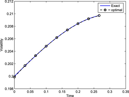
First we assume the true volatility function ${\sigma }_{ex}(t)$ is defined as: ${\sigma }_{ex}(t)=0.2+\frac{\sin (5t)}{100},t\in [0,0.3].$ The recovered volatility and true volatility are presented in Figure 1. It can be observed that the recovered values coincide with the exact values almost perfectly. This verifies the effectiveness of our proposed method.

Figure 1. Volatility estimation with entropy binomial tree.

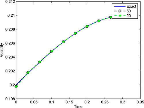
To investigate the stability of our algorithm, we add white noise to the observed data. We set: $C_{mkt}^{\ast }=(1+\frac{\xi }{\delta })C_{mkt},$ where ξ is a random variable drawn from the standardized normal distribution, $\delta =50,20$. Then we use $C_{mkt}^{\ast }$ to reconstruct the local volatility. The results, presented in Figure 2, verify the stability of our algorithm.

Figure 2. Stability analysis of the algorithm.

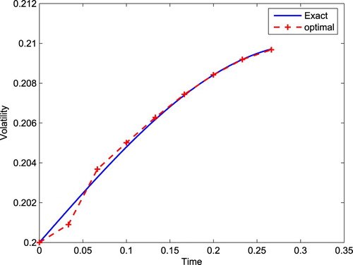
In addition, we compare the calibration results by entropy binomial tree method with traditional binomial tree method. From Figures 1 and 3, we can see that the proposed method is better than the binomial tree method. This is because we smooth the payoff function and obtain unbiased non-negative parameter in entropy binomial tree.

Figure 3. Volatility estimation with binomial tree.

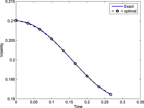
Now we consider the true volatility function ${\sigma }_{ex}(t)$ as follows: ${\sigma }_{ex}(t)=0.2+\frac{\cos (10t)}{100},t\in [0,0.3].$

The comparison between the true volatility and the estimated volatility with n = 10 are shown in Figure 4. We can see that our algorithm still performs well. Similar to the above example, we add white noise to the observed data with the following form to investigate the stability of our algorithm: $C_{mkt}^{\ast }=C_{mkt}+{\delta }_1\xi ,$ where ξ is a random variable drawn from the standardized normal distribution, ${\delta }_1=0.01,0.05$. The comparison between the true volatility and the reconstructed volatility functions with adding noise to observed prices are presented in Figure 5. The results in Figure 5 verify the stability of our method.

Figure 4. Volatility estimation with entropy binomial tree.

5.2. Market tests

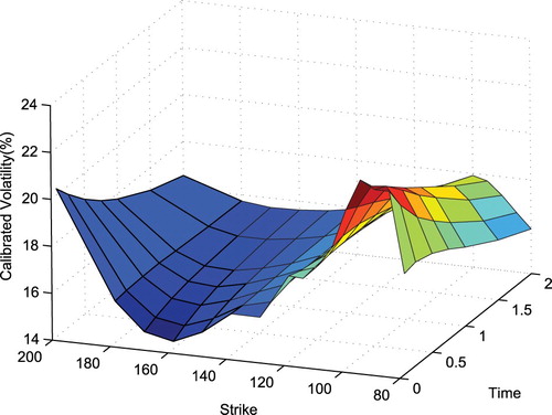
In this section we test the performance of our new method with real market data from S&P 500 index which is described in [31]. The initial index is $S_0=1306.17$, the risk free rate is r = 0.0559. The strike prices and maturity dates as follows $\begin{array}{rl}K/S_0& =[80\mathrm{\%},85\mathrm{\%},90\mathrm{\%},95\mathrm{\%},100\mathrm{\%},105\mathrm{\%},110\mathrm{\%},115\mathrm{\%},\\ & 120\mathrm{\%},130\mathrm{\%},140\mathrm{\%},150\mathrm{\%},160\mathrm{\%},170\mathrm{\%},180\mathrm{\%},200\mathrm{\%}],\\ T& =[0.08,0.25,0.5,0.75,1,1.5,2].\end{array}$ We construct the implied entropy binomial tree with n = 10 for different strike prices and calibrate the volatility. Figure 6 shows the local volatility of the market data. For a fixed strike price, we can obtain a set of discrete points of volatility. Figures 7 and 8 show the interpolated volatility and calibrated volatility at $K/S_0=115\mathrm{\%},130\mathrm{\%}$. The difference in Figure 7 may be caused by the smoothness of volatility or the discretization. Figure 9 reports the interpolated calibrated result. This indicates that our algorithm is effective.

Figure 5. Stability analysis of the algorithm.

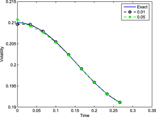
Figure 6. Local volatility surface.

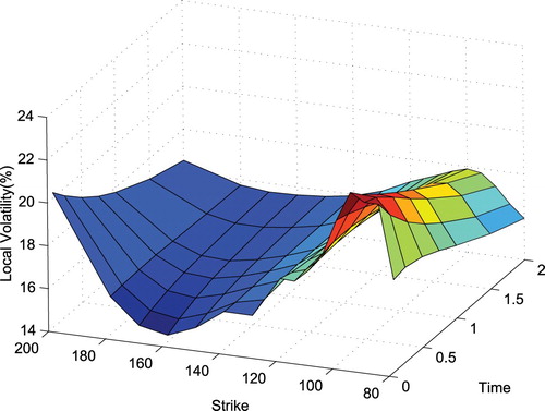
Figure 7. Interpolated local volatility and calibrated volatility at $K/S_0=115\mathrm{\%}$.

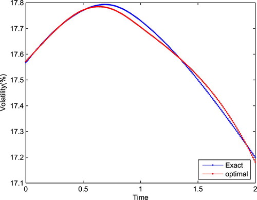
Figure 8. Interpolated local volatility and calibrated volatility at $K/S_0=130\mathrm{\%}$.

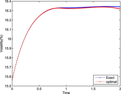
Figure 9. Calibrated volatility surface.

6. Conclusions

In this paper, we develop a new method to reconstruct the volatility from the market data. We first propose an entropy binomial tree pricing model, and present its convergence rates. Then we use the entropy binomial tree to calibrate the volatility smile. The volatility calibration problem under consideration is a optimization problem with nonlinear constraints. We further adopt a penalty method and use quasi-Newton algorithm for the optimization. An extensive numerical analysis is presented to demonstrate the efficiency of our numerical algorithm. It is worthwhile to point out the calibrated volatility coincides very well with the true volatility. Moreover, we test our model using S&P 500 index options data. The results obtained strongly support our modelling approach.

Disclosure statement

No potential conflict of interest was reported by the author(s).

Additional information

Funding

The work is supported by National Natural Science Foundation of China [grant number 11571365].

References

- Black F, Scholes M. The pricing of options and corporate liabilities. J Pol Econ. 1973;81(3):637–654. doi: 10.1086/260062
- Boyle PP. Options: a Monte Carlo approach. J Financ Econ. 1997;4:323–338. doi: 10.1016/0304-405X(77)90005-8
- Cox JC, Ross SA, Rubinstein M. Option pricing: a simplified approach. J Financ Econ. 1979;7:229–263. doi: 10.1016/0304-405X(79)90015-1
- Brennan M, Schwartz ES. Finite difference methods and jump processes arising in the pricing of contigent claims: a synthesis. J Financ Quant Anal. 1978;13:464–474.
- Chance DM. A synthesis of binomial option pricing models for lognormally distributed asset. J Appl Finance. 2008;18:38–56.
- Diener F, Diener M. Asymptotics of the price oscillations of a European call option in a tree model. Math Finance. 2004;14:271-–293. doi: 10.1111/j.0960-1627.2004.00192.x
- Rendleman J, Richard J, Bartter BJ. Two-state option pricing. J Finance. 1979;34:1093–1110. doi: 10.1111/j.1540-6261.1979.tb00058.x
- Walsh JB. The rate of convergence of the binomial tree scheme. Finance Stoch. 2003;7:337–361. doi: 10.1007/s007800200094
- Li YH, Li XS. Entropy binomial tree model for option pricing. Appl Math Inf Sci. 2013;7(1):151–159. doi: 10.12785/amis/070118
- Jaynes ET. Information theory and statistical mechanics. Phys Rev. 1957;106:620–630. doi: 10.1103/PhysRev.106.620
- Dupire B. Pricing with a smile. Risk. 1994;7:18–20.
- Bouchouev I, Isakov V. Uniqueness, stability and numerical methods for the inverse problem that arises in financial markets. Inverse Probl. 1999;15:95–116. doi: 10.1088/0266-5611/15/3/201
- Hofmann B, Kramer R. On maximum entropy regularization for a specific inverse problem of option pricing. J Inverse Ill-Posed Probl. 2005;13:41–63. doi: 10.1515/1569394053583739
- Wang Y, Zhang Y, Lukyanenko D, et al. Recovering aerosol particle size distribution function on the set of bounded piecewise-convex functions. Inverse Probl Sci Eng. 2013;21:339–354. doi: 10.1080/17415977.2012.700711
- Jiang LS, Bian BJ. The regularized implied local volatility equations-A new model to recover the volatility of underlying asset from observed market option price. Discrete Continuous Dyn Syst, Ser B. 2012;7(6):2017–2046. doi: 10.3934/dcdsb.2012.17.2017
- Korolev YM, Kubo H, Yagola AG. Parameter identification problem for a parabolic equation – application to the Black–Scholes option pricing model. J Inverse Ill-Posed Probl. 2012;20:327–337.
- Wang YF. Computational methods for inverse problems and their applications. Beijing: Higher Education Press; 2007.
- Atkinson K. An introduction to numerical analysis. 2nd ed. New York (NY): John Wiley & Sons; 1989.
- Li Y. A new algorithm for constructing implied binomial trees: does the implied model fit any volatility smile? J Comput Finance. 2001;4:69–98. doi: 10.21314/JCF.2001.072
- Derman E, Kani I, Chriss N. Implied trinomial trees of the volatility smile. J Deriv. 1996;3:7–22. doi: 10.3905/jod.1996.407952
- Barle S, Cakici N. How to grow a smiling tree. J Financ Eng. 1999;7:127–146.
- Crépey S. Calibration of the local volatility in a trinomial tree using Tikhonov regularization. Inverse Probl. 2003;19:91–127. doi: 10.1088/0266-5611/19/1/306
- Talias K. Implied binomial trees and genetic algorithms [Ph.D. thesis]. Imperial College; 2005.
- Charalambous C, Christofides N, Constantinide E, et al. Implied non-recombining trees and calibration for the volatility smile. Quant Finance. 2007;7(4):459–472. doi: 10.1080/14697680701488692
- Lok UH, Lyuu YD. The waterline tree for separable local-volatility models. Comput Math Appl. 2017;73:537–559. doi: 10.1016/j.camwa.2016.12.008
- Gong WX, Xu ZL. Non-recombining trinomial tree pricing model and calibration for the volatility smile. J Inverse Ill-Posed Probl. 2019;27(3):353–366. doi: 10.1515/jiip-2018-0005
- Li XS. An efficient approach to nonlinear minimax problems. Chin Sci Bull. 1992;37(10):802–805.
- Heston S, Zhou GF. On the rate of convergence of discrete-time contingent claims. Math Finance. 2000;10(1):53–75. doi: 10.1111/1467-9965.00080
- Fiacco AV, McCormick GP. Nonlinear programming: sequential unconstrained minimization techniques. New York (NY): John Wiley & Sons; 1968.
- Fletcher R. Practical methods of optimization. Chichester: Wiley; 1987.
- Andersen L, Andreasen J. Jump-diffusion processes: volatility smile fitting and numerical methods for option pricing. Rev Derivat Res. 2000;4:231–262. doi: 10.1023/A:1011354913068