Numerical reconstruction of two-dimensional particle size distributions from laser diffraction data

Abstract

In this paper, we consider the two-dimensional Fredholm integral equation of the first kind. The kernel of this equation models the scattering of a laser beam by spheroids having the same fixed orientation. The unknown function under the integral describes the distribution of spheroids along two semi-axes. The input data are the diffraction pattern corresponding to the scattering of the laser beam by the particles. We show that the Tikhonov regularization method allows one to reconstruct two-dimensional distributions in the case when the diffraction pattern is modulated by white noise with relative amplitude up to 1%. In applications, this means novel possibility of obtaining two-dimensional particle size distributions, rather than one-dimensional ones, as in the classical version of the method. This significantly expands the capabilities of particle sizing via static laser diffraction technique. We show that the solution of the corresponding equation is unique in $L_2$ space and exists when the right-hand-side function is in a set dense in $L_2$. We provide test experimental results in the framework of laser ektacytometry of red blood cells, which serves as the main application of the proposed approach presently.

KEYWORDS:

• Particle sizing
• Fredholm equation
• inverse problem
• Tikhonov regularization
• laser ektacytometry

2010 MATHEMATICS SUBJECT CLASSIFICATION:

• 45B05

1. Introduction

Currently, laser light diffraction measurements are massively used to obtain small particle size distributions in a wide variety of scientific and technical fields. Using this technique, the sizes of microorganisms in ocean and river water, the dispersion of powder medicines in manufacturing, agglomerates of dust particles in emissions of combustion products are investigated, and quality control of cement production and small paint balls is carried out – see review [1].

In the classical method, each particle is modelled using a homogeneous sphere of equivalent volume [1]. Laser beam illuminates the particles and diffraction of light is observed in the far-field diffraction zone. The angular distribution of the intensity of the scattered light is called a diffraction pattern. The angle of observation is the angle of deviation from the linear propagation of the laser beam.

From the mathematical point of view, the laser beam is an incident plane monochromatic wave. Usually the wavelength is chosen from the visible emission spectrum. For the correct application of the approximations used in the present work, it is necessary that the particles have dimensions that coincide with the wavelength, or one or several orders of magnitude larger than it. Thus, the approximation of anomalous diffraction will be applicable for calculating the scattering of light by a single particle. For smaller particles, the Gans–Debye approximation should be used, and for larger particles, the geometric optics approximation should be used.

In the classical method, the following equation is widely used to reconstruct the distribution of particle sizes, see for example [1] (chapter 3) and [2]: (1) ${\int }_0^{\mathrm{\infty }}{\left(\frac{J_1(kr\theta )}{kr\theta }\right)}^2{r}^4\omega (r)\text{d}r=I(\theta ),$(1) where $\theta$ is the observation angle in radians, should be set from zero to $\frac{\pi }{6}$. $k=\frac{2\pi }{\lambda }$ is the wavenumber of the incident wave. $r$ is the radius of the particle-sphere. $I(\theta )$ is the diffraction pattern described by one variable due to the fact that in this case, the diffraction pattern has an ideal circular symmetry. $J_1$ is the Bessel function of the first kind of the first order. $\omega (r)$ is the particle size distribution, which is to be found from the function $I(\theta )$ measured in the experiment. The kernel with the Bessel function approximately describes the scattering of light by a single sphere with radius $r$.

The angle $\theta$ can be expressed in terms of the Cartesian coordinates using the equation $\frac{x}{z}=\tan \theta \approx \theta$, where $x$ is the Cartesian coordinate of the observation point, $z$ is the distance from the observation plane to some small volume containing all the particles illuminated by the laser. Such a large value of angle $\theta =\pi /6$ should be taken carefully. As described in chapter 2 of the book [1], this is a suitable assumption only for particles which are bigger than the laser wavelength not more than by 1 order. The erythrocytes in laser ektacytometry meet this requirement.

In a number of papers, some authors tried to generalize the method of laser diffractometry to obtain not only the radii of particles but also the distribution in the elongations. We mention the initial paper [3], as well as subsequent clarifying and complementary ones [4,5]. However, in all these papers, it was necessary to fix the number of illuminated particles in order for their orientation to have a controlled degree of randomness. The basis for solving the inverse problem was the statistical correlation between random fluctuations in the diffraction pattern and the distribution of particles along the elongations. Thus, a full-fledged theory based on integral equations was not derived in these works, and the orientation of the particles in the incident field was random.

In paper [6], a similar inverse problem was considered. The spheroids were used to model a gravitational potential and corresponding inverse problem was solved by means of Tikhonov regularization.

Note the recent publication [7], where the distribution of random-oriented spheroids in their two characteristic sizes is reconstructed from the extinction spectrum of scattered light. In this paper, the corresponding integral equation is given, but for such measurements, it is necessary to illuminate particles with a source containing several wavelengths in order to obtain a spectrum of scattered light. The approach proposed in the present article differs significantly in that we assume the light scattering for one fixed and a priori known wavelength. We also note that measurements of light scattering at large angles and measurements based on a change in the polarization of the incident light wave are beyond the scope of our paper.

Let us mention the erythrocyte laser ektacytometry technique, which has been historically developed in parallel with the classical particle sizing. In the ektacytometry, red blood cells are placed in a special shear flow, which stretches red blood cells and gives them the same orientation. The elongation of erythrocytes under the action of a known external force serves as a characteristic of their deformability, or, equivalently, elasticity. This information is valuable for medical blood diagnostics in the case of a number of socially significant diseases, see for example [8].

Laser ektacytometry uses an integral relation similar to (1), but written for the case of elongated particles. Usually, based on it, only the average elongation of blood cells is assessed from a measured diffraction pattern. Only a few recent works propose to extract information not only about the first moment of distribution, but also about the second moment [9,10] and the third moment [11,12]. Recently in [11], it was proposed to use this relation as an integral equation to determine the unknown distribution function of erythrocytes in their elongations. However, in all mentioned papers, it was assumed that all particles have the same and a priori known area; therefore, the distribution was essentially a function of one variable. In the present work, for the first time, it is proposed to abandon this restriction and consider the problem in a completely two-dimensional formulation, when the distribution $\omega (a,b)$ is a function of two independent characteristic sizes $a$ and $b$. Let us write the corresponding equation: (2) ${\int }_0^{+\mathrm{\infty }}{\int }_0^{+\mathrm{\infty }}{a}^2{b}^2{\left(\frac{J_1\left(\frac{k}{z}\sqrt{x^2{a}^2+y^2{b}^2}\right)}{\frac{k}{z}\sqrt{x^2{a}^2+y^2{b}^2}}\right)}^2\omega (a,b)\text{d}a\text{d}b=I(x,y),$(2) where all quantities are similar to those in Equation (1); $x,y$ is a point in the plane of observation.

In this article, we introduce a priori constraints that allow us to consider equation (2) under conditions close to real practice, when particles cannot have infinitely large or infinitely small sizes, and the observation area is limited to a relatively small rectangle. Thus, the following holds: (3) ${\int }_{b^{\mathrm{\prime }}}^{b^{\mathrm{\prime }\mathrm{\prime }}}{\int }_{a^{\mathrm{\prime }}}^{a^{\mathrm{\prime }\mathrm{\prime }}}{a}^2{b}^2{\left(\frac{J_1\left(\frac{k}{z}\sqrt{x^2{a}^2+y^2{b}^2}\right)}{\frac{k}{z}\sqrt{x^2{a}^2+y^2{b}^2}}\right)}^2\omega (a,b)\text{d}a\text{d}b=I(x,y),$(3) $x\in [x^{\mathrm{\prime }},x^{\mathrm{\prime }\mathrm{\prime }}],y\in [y^{\mathrm{\prime }},y^{\mathrm{\prime }\mathrm{\prime }}]$

Here the values $a^{\mathrm{\prime }},a^{\mathrm{\prime }\mathrm{\prime }},b^{\mathrm{\prime }},b^{\mathrm{\prime }\mathrm{\prime }},x^{\mathrm{\prime }},x^{\mathrm{\prime }\mathrm{\prime }},y^{\mathrm{\prime }},y^{\mathrm{\prime }\mathrm{\prime }},k,z$ are fixed a priori known constants.

The main aim of this paper is the mathematical formulation of the problem corresponding to Equation (3), as well as its numerical solution using the Tikhonov regularization method in the case when a term containing noise of certain amplitude is added to the right--hand side $I(x,y).$

We also aim to study uniqueness and existence of solution of Equation (2). We consider more practical Equation (3) as a modification of (2), when solution has finite a priori known support and right hand is taken in some finite fixed area at the plane of observation.

The basic physical condition for the applicability of Equation (3) in practice is that the particles should have the same and fixed orientation along parallel lines. In laser ektacytometry, erythrocytes are oriented in the same direction due to the action of shear flow; therefore, Equation (3) proposed in this article can be applied directly without any modification of existing devices. In other laser diffraction devices, which model is based on classic Equation (1), it is necessary to place the particles in an external field, which would give them the same orientation. In particular, elongated dielectric particles can be oriented along parallel lines simply by placing them in a constant electric field.

Thus, the proposed new Equation (3) makes it possible to generalize the method of measuring particle size distributions according to laser diffraction data from the one-dimensional to the two-dimensional case. In the case of laser ektacytometry, this will lead to more accurate and informative medical blood tests. At the same time, this will allow to bring all other measurements of the characteristics of dispersed suspensions and powders to a fundamentally new level, which, of course, confirms the relevance of this work.

2. Uniqueness and existence of solution

Consider integral Equation (2) with infinite limits of integration and an infinite domain of the function. Let us rename the unknown function to ${\omega }_2(a,b)=a^2{b}^2\omega (a,b)$. The resulting equation is a two-dimensional Mellin convolution-type equation, because its kernel depends only on the product of its arguments: $K(x,y,a,b)=K(xa,yb)$

For equations of this type, the convolution theorem holds, which states that the Mellin transform of the convolution is the product of the Mellin transform of the kernel function and the solution function: $\tilde{K}(s_1,s_2)\cdot \widetilde{{\omega }_2}(-s_1,-s_2)=\tilde{I}(s_1,s_2),s_1,s_2\in \mathbb{R},$where symbols with tilde hats denote the Mellin transform of the corresponding functions. For our kernel, by direct integration, using the Weber Schafheitlin integral and the definition of the Beta function, we obtain $\tilde{K}(s_1,s_2)=\frac{\mathrm{\Gamma }\left(\frac{1}{4}+i\cdot \frac{s_1}{2}\right)\mathrm{\Gamma }\left(\frac{1}{4}+i\cdot \frac{s_2}{2}\right)}{2}\cdot \frac{2^{-2+i\cdot (s_1+s_2)}\mathrm{\Gamma }(2-i\cdot (s_1+s_2))}{{\mathrm{\Gamma }}^2\left(\frac{3}{2}-i\cdot \frac{(s_1+s_2)}{2}\right)\mathrm{\Gamma }\left(2.5-i\cdot \frac{(s_1+s_2)}{2}\right)}$

To the best of the authors’ knowledge, the exact values of the Mellin transform and the arguments for the existence and uniqueness of Equation (2) are provided in the literature for the first time. In the article [2] similar formulas are given, but only in the case of one-dimensional Equation (1). Book [13] describes general technique for the analysis and regularization of convolution-type equations. As one can see, the expression for $\tilde{K}(s_1,s_2)$ is a product of functions that are certainly not equal to zero anywhere, which means that $\tilde{K}(s_1,s_2)\ne 0$ for any $s_1,s_2\in \mathbb{R}$.

We will look for solutions in $L_2({\mathbb{R}}_{+}^2)$. This space is convenient to choose, since it is well known that the Mellin transform translates in a one-to-one way $L_2({\mathbb{R}}_{+}^2)$ into $L_2({\mathbb{R}}^2)$. By direct integration, we can verify that the kernel $K\in L_1({\mathbb{R}}_{+}^2)\bigcap L_{\mathrm{\infty }}({\mathbb{R}}_{+}^2)$. Then, by the well-known property of the Mellin transform: $\tilde{K}\in L_{\mathrm{\infty }}({\mathbb{R}}^2),\widetilde{{\omega }_2}\in L_2({\mathbb{R}}^2),$which means $\tilde{K}\cdot \widetilde{{\omega }_2}=\tilde{I}\in L_2({\mathbb{R}}^2)$. Using the inverse Mellin transform, we conclude that $I\in L_2({\mathbb{R}}_{+}^2)$. That is, our integral operator acts from $L_2({\mathbb{R}}_{+}^2)$ into $L_2({\mathbb{R}}_{+}^2)$.

As we have mentioned earlier, $\tilde{K}(s_1,s_2)\ne 0$ for all $s_1,s_2\in \mathbb{R}$. This means that if for some right-hand side $I\in L_2({\mathbb{R}}_{+}^2)$ there are two solutions, then their difference is zero as a function of $L_2({\mathbb{R}}_{+}^2)$. This is due to that after taking the Mellin transform of equation (2) with zero right-hand-side we have $\tilde{K}(s_1,s_2)\cdot \widetilde{{\omega }_{zero}}(-s_1,-s_2)=0,$and we can divide by $\tilde{K}(s_1,s_2)\ne 0$ at all points. Thus, the solution of homogeneous problem ${\omega }_{zero}(a,b)$ in $L_2({\mathbb{R}}_{+}^2)$ is constant zero.

A formal solution to the equation can be obtained using the inverse Mellin transform of the function $\tilde{I}(s_1,s_2)/\tilde{K}(s_1,s_2)$ if and only if $\tilde{I}(s_1,s_2)/\tilde{K}(s_1,s_2)\in L_2({\mathbb{R}}^2).$

Due to the properties of the Gamma function, the above-mentioned function $\tilde{K}(s_1,s_2)$ is continuous, bounded, never vanishes, and does not tend to zero anywhere except infinity. Moreover, if we apply the well-known Stirling approximation for each Gamma function from the expression for $\tilde{K}(s_1,s_2)$, it becomes clear that $|\tilde{K}(s_1,s_2)|$tends to zero with the speed of a polynomial of $(s_1,s_2)$ of a fixed degree. This means that the image of our integral operator contains all the functions $I(x,y)\in L_2({\mathbb{R}}_{+}^2)$, with $\tilde{I}$ decreasing at infinity faster than the indicated polynomial squared. The set of such functions is everywhere dense in$L_2({\mathbb{R}}_{+}^2)$. Thus, a solution in$L_2({\mathbb{R}}_{+}^2)$ exists for a wide enough class of functions from $L_2({\mathbb{R}}_{+}^2)$.

Below, we consider Equation (3), similar to Equation (2), but in a finite region. From the standpoint of the general theory, one can consider this truncation as introducing errors into the right-hand side of $I(x,y)$ and into the integral operator. We lose some information, but not too much in view of the fact that for the solutions of interest to us, the exact right-hand side decreases fast and becomes very small at observation angles greater than $\pi /6$.

For convolution-type equations, there are special regularizing operators based on a modification of the inverse Mellin transform, see, for example, [13]. However, in this paper we will use classical regularization in view of the fact that it allows us to choose arbitrary set of points in the input data. This is important, because in natural experiments, the right side is not available in the rectangle, but only in a small area of irregular shape.

3. Problem statement and numerical method

In this paper, we consider the integral Equation (3). For convenience, we denote the integral operator from the left side of this equation by $A$ as follows: $(A\omega )(x,y)={\int }_{b^{\mathrm{\prime }}}^{b^{\mathrm{\prime }\mathrm{\prime }}}{\int }_{a^{\mathrm{\prime }}}^{a^{\mathrm{\prime }\mathrm{\prime }}}{a}^2{b}^2{\left(\frac{J_1\left(\frac{k}{z}\sqrt{x^2{a}^2+y^2{b}^2}\right)}{\frac{k}{z}\sqrt{x^2{a}^2+y^2{b}^2}}\right)}^2\omega (a,b)\text{d}a\text{d}b,$

The kernel of this operator is continuous due to the fact that the division by zero does not give rise to a singularity because of the well-known limit of the Bessel function at zero. Then the operator is compact if we define the following function spaces: $A:L_2([a^{\mathrm{\prime }},a^{\mathrm{\prime }\mathrm{\prime }}]\times [b^{\mathrm{\prime }},b^{\mathrm{\prime }\mathrm{\prime }}])\to L_2([x^{\mathrm{\prime }},x^{\mathrm{\prime }\mathrm{\prime }}]\times [y^{\mathrm{\prime }},y^{\mathrm{\prime }\mathrm{\prime }}]),$

Thus, in this paper we will solve the equation $(A\omega )(x,y)=I(x,y),$ $\omega (a,b)\in L_2([a^{\mathrm{\prime }},a^{\mathrm{\prime }\mathrm{\prime }}]\times [b^{\mathrm{\prime }},b^{\mathrm{\prime }\mathrm{\prime }}]),I(x,y)\in L_2([x^{\mathrm{\prime }},x^{\mathrm{\prime }\mathrm{\prime }}]\times [y^{\mathrm{\prime }},y^{\mathrm{\prime }\mathrm{\prime }}])$

Let us define the values of all the constants for further use: $k=\frac{2\pi }{\lambda },\lambda =0.63,$ $a^{\mathrm{\prime }}=b^{\mathrm{\prime }}=0,a^{\mathrm{\prime }\mathrm{\prime }}=b^{\mathrm{\prime }\mathrm{\prime }}=15,$ $x^{\mathrm{\prime }}=y^{\mathrm{\prime }}=0,\frac{x^{\mathrm{\prime }\mathrm{\prime }}}{z}=\frac{y^{\mathrm{\prime }\mathrm{\prime }}}{z}=\frac{\pi }{10},$ $z=5\cdot {10}^3$

All values used here are given in microns. The choice of $z$ and $k$, as can be seen from the form of the equation, affects only the scaling of the characteristic quantities. We have chosen the domain of the $\omega (a,b)$ taking into account possible erythrocyte elongations in the laser ektacytometry technique, which currently serves as a major application.

The kernel of the integral Equation (3) is a function that describes the scattering of light by a single particle. In this case, such a function was obtained by using the anomalous diffraction approximation for the case of spheroid with the semi-axes $a$ and $b$. The anomalous diffraction approximation holds true only in small observation angles. The ratio $\frac{x^{\mathrm{\prime }\mathrm{\prime }}}{z}$ determines the maximum angle of observation of the diffraction pattern in radians: $\frac{\pi }{10}=\frac{x^{\mathrm{\prime }\mathrm{\prime }}}{z}=\tan (\theta )\approx \theta$. Thus, in degrees the value of $\theta \approx 18$, which corresponds well to the case of small angles.

To regularize Equation (3), we apply classical Tikhonov regularization method. We will only search for non-negative solutions $\omega (a,b)$, because the desired function is the size distribution of particles. Thus, we need to find: (4) ${\omega }_{\alpha }=\underset{L_2([a^{\mathrm{\prime }},a^{{}^{\mathrm{\prime }\mathrm{\prime }}}]\times [b^{\mathrm{\prime }},b^{{}^{\mathrm{\prime }\mathrm{\prime }}}])}{\text{argmin}}\parallel A\omega -I_{\delta }{\parallel }_{L_2}^2+\alpha \parallel \omega {\parallel }_{L_2}^2\text{when}\omega \ge 0$(4) where $I_{\delta }(x,y)$ is the function of the right-hand side, measured in the experiment. Its norm differs from the original by the known constant $\delta =\parallel I-I_{\delta }{\parallel }_{L_2}$. $\alpha >0$ is the regularization parameter.

The Tikhonov functional in (4) is strongly convex. The set of non-negative functions in $L_2$ is also convex and closed. It is well known that the functional has a unique minimum in such a set.

To solve this problem, one can apply many appropriate iterative methods. In particular, we used quadratic programming techniques, namely interior point method and trust region reflective method. We also compared them with the gradient projection method. The interior point method proved to be better than the others; therefore, we present its results in the next section.

In order to program these methods, it is necessary to introduce grids of points and a matrix approximation of the operator and of the right-hand side.

Consider a uniform grid for the values of the variables $x,y$ with the number of points $N$ along each axis: $x_i=x^{\mathrm{\prime }}+\frac{i-1}{N-1}\cdot (x^{\mathrm{\prime }\mathrm{\prime }}-x^{\mathrm{\prime }}),y_j=y^{\mathrm{\prime }}+\frac{j-1}{N-1}\cdot (y^{\mathrm{\prime }\mathrm{\prime }}-y^{\mathrm{\prime }})$

Based on it, we introduce a discrete analogue of the operator $A$ and denote it by $A_h$: $A_h{\omega }_h=\sum _{m=1}^M\sum _{n=1}^M\frac{(b^{\mathrm{\prime }\mathrm{\prime }}-b^{\mathrm{\prime }})}{M-1}\frac{(a^{\mathrm{\prime }\mathrm{\prime }}-a^{\mathrm{\prime }})}{M-1}{a}_m^2{b}_n^2{\left(\frac{J_1\left(\frac{k}{z}\sqrt{x_i^2{a}_m^2+y_j^2{b}_n^2}\right)}{\frac{k}{z}\sqrt{x_i^2{a}_m^2+y_j^2{b}_n^2}}\right)}^2\omega (a_m,b_n),$ $a_m=a^{\mathrm{\prime }}+\frac{m-1}{M-1}\cdot (a^{\mathrm{\prime }\mathrm{\prime }}-a^{\mathrm{\prime }}),b_n=b^{\mathrm{\prime }}+\frac{n-1}{M-1}\cdot (b^{\mathrm{\prime }\mathrm{\prime }}-b^{\mathrm{\prime }})$

Let us denote the discrete analogue of right-hand side by $I_h$ and the same quantity with noise by $I_{h_{\delta }}$.

We also consider minimization of the Tikhonov functional without restrictions. Then, equating the gradient of the functional to zero leads to the Euler equation with unknown vector ${\omega }_h$: (5) $(A_h^T{A}_h+\alpha E){\omega }_h=A^T{I}_{h_{\delta }},$(5) where $E$ is the identity matrix and $\alpha >0$ is the regularization parameter. One can treat (5) as a system of linear equations until its size is not too high. Otherwise, it is better to apply iterative methods to perform minimization of Tikhonov functional. Numerically, this minimization in terms of quadratic programming techniques can be written as follows: $\underset{{\omega }_h}{\text{find argmin}}0.5\cdot {\omega }_h^T(A_h^T{A}_h+\alpha E){\omega }_h-I_{h_{\delta }}^T{A}_h{\omega }_{h,}\text{when}\omega \ge 0$

Note the peculiarity of the numerical record of the matrix $A_h$ indicated above and the set of values of the vectors ${I_h}_{\delta }$ and ${\omega }_h$ corresponding to functions $I_{\delta }(x_i,y_j),\omega (a_m,b_n)$. Each point $x_i,y_j$ adds one equation to the system. Therefore, in order to list the initially two-dimensional set of quantities in a one-dimensional format, a new index was introduced: $l=i+N\cdot (j-1),$Thus, we obtain sizes of matrices for computer program $\dim A_h=N^2\times M^2$ and $\dim {\omega }_h={\text{M}}^2\times 1,\text{ dim}{I}_{h_{\delta }}=N^2\times 1$.

We briefly indicate that for a given noise $\delta$, the regularization parameter $\alpha$ was chosen in accordance with the principle of the generalized discrepancy, as it is described in [14].

4. Numerical results and discussion

To test the regularization algorithm, 3 main erythrocyte distribution functions were used, which are relevant from the point of view of application in laser ektacytometry: ${\omega }_s(a,b)=p_{s1}\cdot e^{-\frac{{(a-A_1)}^2+{(b-B_1)}^2}{{\sigma }_1^2}}+p_{s2}\cdot e^{-\frac{{(a-A_2)}^2+{(b-B_2)}^2}{{\sigma }_2^2}},$ $p_{s1}=\{\begin{array}{l}0.2,s=1;\\ 0.5,s=2;\\ 0.8,s=3;\end{array}$ $p_{s2}=\{\begin{array}{l}0.8,s=1;\\ 0.5,s=2;\\ 0.2,s=3;\end{array}$ $A_1=4,B_1=4,A_2=6.3,B_2=2.5,$ ${\sigma }_1=0.8,{\sigma }_2=0.8$

The $p_1,p_2$ values are dimensionless, the other values, as before, are given in microns. The functions selected for the analysis consist of two components imitating fractions of particles elongated in different ways. Inside each fraction, there is some heterogeneity, due to the width of the normal distribution.

Case of $s=2$ is shown in Figure 1. The values of $(A_1,B_1),(A_2,B_2)$ are the centres of the two Gaussian functions. ${\sigma }_1$ and ${\sigma }_2$ correspond to their width. The choice of $A_1=B_1$ illustrates real situation in which some of the cells are sick and do not elongate at all. There is part of such hard cells in the case of sickle cell disease, spherocytosis, tropical malaria and a number of other socially important diseases, see [15]. The rest of the cells are normal and elongate according to the value of pressure applied to the liquid. Here, we choose $A_2/B_2=2.5$ imitating typical pressure value in Rheoscan ektacytometer, which we consider in the next section.

Figure 1. The correct distribution $\omega (a,b)$.

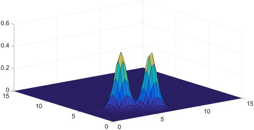
For illustration, we consider the case of $s=2$. At this $s$ value, the distribution contains two components with equal weights $0.5=p_{21}=p_{22}$. Results in the remaining cases were generally similar.

All the numerical results presented in this section were obtained by using Matlab Mathworks software package. As it was described in the previous section, we performed minimization (4) of Tikhonov functional applying different methods. We applied two quadratic programming techniques - interior point method and trust region reflective method. Furthermore, we programmed the gradient projection method. We also tried to solve Euler Equation (5) as a SLAE in the case when the dimension of matrix was less then 500 by means of the Gauss method.

We managed to achieve the best results with the help of the interior point method provided that the function is non-negative. We show the results of application of this method in Figures 1–3. Figure 1 shows the true solution which was set in advance and with which one should compare Figures 2 and 3. In Figures 1–3 the value of $N$ was 50 and $M$ was 200 and the maximum angle of observation was $\pi /10$.

Figure 2. The result of performing minimization (4) in the case of 10% noise amplitude.

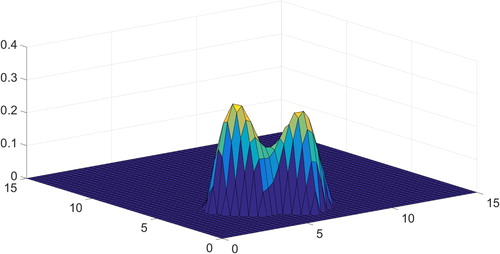
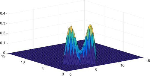
Figure 3. The result of performing minimization (4) in the case of 1% noise amplitude.

In order to perform a numerical test experiment, we calculated right hand-side $I_h$ applying $A_h$ matrix to the correct solution vector. Then we added generated uniform random noise vector to it and obtained $I_{h_{\delta }}$. We describe the noise by fixed percent value, which is the maximum of $100\mathrm{\%}\cdot \frac{|I_{h_{\delta }}-I_h|}{I_h}$ at each point.

In modern laser particle sizers, the noise is greatly reduced due to the use of precise sensors, vacuum chambers, etc. However, in ektacytometry, which serves as a main application for now, the noise value can be more than $1\mathrm{\%}$.

Figure 2 contains the result of minimization (4) with random noise added to the right-hand side with an amplitude of 10% relative to the true signal.

Figure 3 shows the result of minimization (4) with random noise added to the right-hand side with an amplitude of 1% relative to the true signal. The regularization parameter $\alpha$ was found via general discrepancy principle and turned out to equal about 0.1 in the case of big noise (Figure 2) and about 0.01 in the case of lower noise (Figure 3).

One can see that the two-dimensional solution $\omega (a,b)$ is reconstructed and it is comparable with a predetermined standard, shown in Figure 1. The centres of the two peaks $A_1,B_1,A_2,B_2$ and the values of their widths ${\sigma }_1,{\sigma }_2$ are restored with acceptable accuracy in both cases. The ratio of these peaks was found to be $p_{21}:p_{21}\approx 0.9-0.99$ in the case of 10% noise and in the case of 1% noise.

However, the value of the function at the minimum deflection between two peaks with respect to the maximum of the entire function is 0.1 for the true solution, 0.3 for 1% noise and 0.6 for 10% noise.

It is also of interest what information can be obtained from the data that is currently available in existing ektacytometers. The following section is devoted to this.

5. Laser ektacytometry experiment

In order to test the proposed method experimentally, we used the Rheoscan [16] laser erythrocyte ektacytometer available in the biophotonics laboratory of the Physics Department of Lomonosov Moscow State University. A shear flow is created in the device, orienting and elongating red blood cells. A laser beam illuminates elongated cells and light scattered at small angles is recorded on a CCD matrix. The maximum observation angle is about 7 degrees. The camera resolution is 640 by 480, the dynamic range is about 1:100.

The blood of a healthy donor of a 29-year-old man was used with his informed and voluntary consent.

In the case of sickle cell anemia as well as several other diseases, some of the cells are rigid and do not stretch at all in a shear flow, see, for example, [15]. To simulate this situation, we treated a previously known part of the blood cells with glutaraldehyde. This substance fixes the cytoskeleton of red blood cells and makes them rigid. The remaining red blood cells were left normal. Thus, we obtained a mixture of hard and normal cells, and the proportion is known in advance. This allows us to conduct test experiments in order to verify the approach proposed in this article in practice.

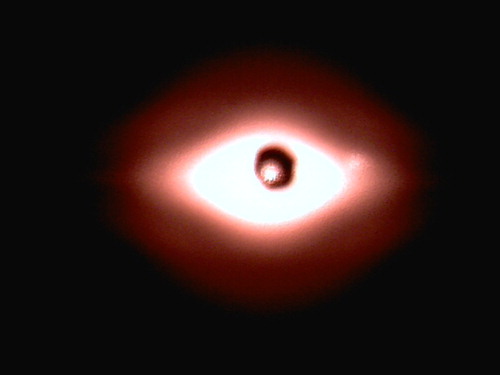
Figure 4 shows the diffraction pattern measured in a real experiment in the case when the mixture of cells contained equal amount of rigid and normal red blood cells. One can see that in the centre of the picture there is a dark spot that removes a direct laser beam. In arbitrary units, the intensity formally passes values from 0 to 255. On the sides of the picture, the intensity is so small that in the computer's memory it is recorded as constant 7 which means that it can not be used as an input data in our program. In order to extract useful part of the signal, we selected those points where the intensity was from 15 to 210. Due to the symmetry of the picture relative to the centre point, one could select any quarter of the image. We chose the lower left quarter, as there were no light flare and other obvious defects in it.

Figure 4. Diffraction pattern detected in Rheoscan in the case of mixture of rigid and normal cells in 1:1 proportion.

In ektacytometry, a standard image processing algorithm is used, which allows one to calculate the average value of red blood cells elongation from given diffraction pattern. The algorithm uses the set of points with equal intensity, which is called isointensity curve. In the case of circular cells, this curve is a circle. When cells are elongated spheroids, this curve also elongates and becomes approximately an ellipse. In practice, the ellipse of best fit is used. Ratio of axes of this ellipse is considered to be equal to average elongation of the cells. This approach is applied in all commercially available ektacytometers presently [17] including Rheoscan.

However, this is a simplification. The algorithm is precise only in the case when absolutely all red blood cells are elongated equally. There are fractions of more hard and more soft cells even in the blood of a healthy person, see [15]. The regularization-based method proposed in this article allows one to obtain the entire two-dimensional distribution of $\omega (a,b)$ without such simplification and also to calculate the average elongation $(a/b)$ more accurately.

We compare averaged value of $(a/b)$ of the function $\omega (a,b)$ found via using regularization algorithm according to minimization (4) with the same $(a/b)$ ratio measured from ratio of axes of ellipse fitted to isointensity curve.

In the case of mixture of hard and normal cells, the average elongation of cells, obtained via ratio of ellipse fitted to the isointensity curve, strongly depends on the level of intensity at which isointensity curve is found. In Rheoscan device, the value about 200 is chosen. At such a high value, isointensity curve is almost not sensitive to the impact of rigid cells. For calculations below, we picked up level of intensity equal to 80 due to the better sensitivity.

Let us denote by ‘A’ case when only hardened erythrocytes treated with glutaraldehyde were measured in Rheoscan. Such cells do not elongate at all. Both regularization algorithm and classical ektacytometry approach applied to the same images gave us $(a/b)=1.0$ at all available pressure values. This confirms that glutaraldehyde, indeed, has made cells completely rigid.

Let ‘B’ stand for the case when there were only normal cells. We consider the pressure value of 5 Pa. In Rheoscan program, the diffraction images are enumerated from 1 to 100 corresponding to decreasing pressure values applied to the fluid in measurement chamber. The pressure value of 5 Pa corresponds to the image number 40. At this value, the classical ektacytometry approach gave average $(a/b)=2.1$ and the regularization algorithm $(a/b)=2.0$. Complete comparison of regularization and standard ektacytometry algorithm is given in Figure 5 on the left. One can see that two independent approaches give close results.

Figure 5. The dashed line shows the average $(a/b)$ value found by regularization. The solid line shows the same value found using the standard ektacytometry method. Case ‘B’ is on the left, it corresponds to normal cells. Case ‘C’ is on the right, it corresponds to the mixture of normal and hard cells in 1 to 1 proportion.

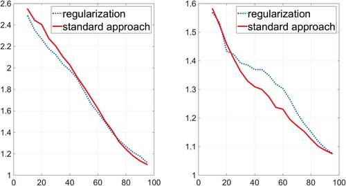
Finally, let ‘C’ denote the case when we mix normal and hardened cells in one-to-one proportion. We took 3 mkl of rigid cells and 3 mkl of normal cells in order to keep amount of cells in a chamber unchanged, i.e. 6 mkl of erythrocytes.

Simple although not precise prediction for the average elongation value at the same 5 Pa pressure is, therefore, $0.5\cdot 1.0+0.5\cdot 2.0=1.5$. This is due to the fact that we already know the elongation of normal cells equal to 2.0 and of hardened cells equal to 1.0. In this case, regularization algorithm led to $(a/b)=1.35$ and standard ektacytometry algorithm gave $(a/b)=1.27$, which is in good agreement with the indicated prediction. The total comparison is given in Figure 5 on the right.

In general, the value of $(a/b)$ found using regularization differed from that found by the standard ektacytometry algorithm by less than 10% in all cases and for all available pressure values in the fluid.

The obtained results are consistent with the prediction of numerical calculations from the previous section. See Figure 6 for typical 2D distributions of function $\omega (a,b)$ found after applying regularization procedure to diffraction patterns obtained from Rheoscan device. Again in Figure 6, letter ‘A’ stands for the case when the blood sample contained only rigid cells. Letter ‘B’ stands for results obtained in the case when there were only normal cells. Letter ‘C’ denotes the situation when both rigid and normal cells were analysed and the proportion was 1 to 1.

Figure 6. The result of performing minimization (4) in the case of mixture of rigid and normal erythrocytes using the diffraction patterns obtained from Rheoscan device. ‘A’ stands for the case of only rigid cells, ‘B’ for the case of only normal cells and ‘C’ stands for the mixture in 1:1 proportion.

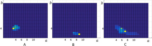
One can see that, as expected in Figure 6 ‘A’ the positive values of the function $\omega (a,b)$ are at the points where $a/b\approx 1$. At the same time, in the case of normal cells ‘B’, positive values are concentrated in the region where $a/b\approx 2.5$ and there are no values for $a/b\approx 1$. This means that all normal cells are elongated under the influence of shear stress. Some of the cells are elongated lower or larger, but completely hard cells in the blood of a healthy donor are not found.

Finally, in the case ‘C’, we had the right to expect overlapping of the figures ‘A’ and ‘B’, because both types of cells were present in solution in equal proportions. Indeed, there is a region of positive values for both $a/b\approx 1$ and $a/b\approx 2.5$. However, the figure shows a peak approximately halfway between them, while two separate peaks were expected, as in theoretical model shown in Figure 1. This means that the ratio between the amount of hard and soft cells cannot be calculated. On the other hand, it was possible to distinguish visually a situation where there were hard cells in the blood from a situation where all cells were normal. This is important diagnostic information.

The numerical calculations presented in the previous section show that in the future, with an increase in the dynamic range of the camera, a decrease in noise, and an increase in the angular view of the camera, it will be possible to distinguish individual peaks of the distribution of $\omega (a,b)$ and obtain more accurate medical diagnostic information.

6. Conclusion

We have numerically shown that distributions of particles in their two characteristic sizes can be reconstructed from the corresponding diffraction patterns with noise added. We have proposed the new Fredholm integral equation as a fundamental model for the method of two-dimensional particle sizing by means of static laser diffraction. We have proved uniqueness of the integral equation solution in $L_2({\mathbb{R}}_{+}^2)$. The existence of the solution is shown in a set dense in $L_2({\mathbb{R}}_{+}^2)$. Both numerical and natural test experiments confirm that numerical instability of the equation can be reduced by using Tikhonov regularization method in its classic formulation. In laser ektacytometry of erythrocytes, our method gives important medical information about the presence of rigid cells in the patients’ blood.

Acknowledgements

The authors thank prof. Razgulin Alexander Vitalyevich from the faculty of the CMC of Lomonosov Moscow State University (MSU), as well as Priezhev Alexander Vasilyevich and Nikitin Sergey Yurievich from the faculty of Physics of Lomonosov MSU for useful discussions.

Disclosure statement

No potential conflict of interest was reported by the author(s).

ORCID

Vladislav D. Ustinov http://orcid.org/0000-0001-5169-4848

Evgeniy G. Tsybrov http://orcid.org/0000-0003-4593-4838

Additional information

Funding

This work was supported by the Russian Science Foundation [grant number 18-71-00158].

References

- Xu R. Particle characterization: light scattering methods. Netherlands: Springer Science & Business Media; 2001. p. 13.
- Bertero M, Pike ER. Particle size distributions from Fraunhofer diffraction. Opt Acta Int J Opt. 1983;30(8):1043–1049. doi: 10.1080/713821332
- Heffels CM, Heitzmann D, Dan Hirleman E, et al. The use of azimuthal intensity variations in diffraction patterns for particle shape characterization // particle & particle systems characterization. Part Part Syst Charact. 1994;11(3):194–199. doi: 10.1002/ppsc.19940110305
- Tinke AP, Carnicer A, Govoreanu R, et al. Particle shape and orientation in laser diffraction and static image analysis size distribution analysis of micrometer sized rectangular particles. Powder Technol. 2008;186(2):154–167. doi: 10.1016/j.powtec.2007.11.017
- Ma Z, Merkus HG, Scarlett B. Extending laser diffraction for particle shape characterization: technical aspects and application. Powder Technol. 2001;118(1–2):180–187. doi: 10.1016/S0032-5910(01)00309-6
- Golov IN, Sizikov VS. Modeling of deposits by spheroids. Izv Phys Solid Earth. 2009;45:258–271. doi: 10.1134/S1069351309030070
- Tang H, Lin JZ. Retrieval of spheroid particle size distribution from spectral extinction data in the independent mode using PCA approach. J Quant Spectrosc Radiat Transfer. 2013;115:78–92. doi: 10.1016/j.jqsrt.2012.09.005
- Priezzhev AV, Tyurina AY, Fadyukova OE, et al. Reduction of erythrocyte deformability in rats with cerebral ischemia. Bull Exp Biol Med. 2004;137(3):313–316. doi: 10.1023/B:BEBM.0000031578.66826.5f
- Streekstra GJ, Dobbe JGG, Hoekstra AG. Quantification of the fraction is poorly deformable red blood cells using ektacytometry. Opt Exp. 2010;18(13):14173–14182. doi: 10.1364/OE.18.014173
- Nikitin S, Ustinov VD. Algorithm of the characteristic point in laser erythrocytometry of erythrocytes. Quantum Elec. 2018;48(1):70–74. doi: 10.1070/QEL16527
- Nikitin S, Priezzhev AV, Lugovtsov AE, et al. Laser ektacytometry and evaluation of red blood cells. J Quant Spectrosc Radiat Transfer. 2014;146:365–375. doi: 10.1016/j.jqsrt.2014.05.012
- Nikitin S, Ustinov VD, Yurchuk YS, et al. New diffractometric equations and data processing algorithm for laser ektacytometry of red blood cells. J Quant Spectrosc Radiat Transfer. 2016;178:315–324. doi: 10.1016/j.jqsrt.2016.02.024
- Tikhonov AN, Ya AV. Methods of solution of Ill-posed problems. Moscow: Nauka; 1979.
- Tikhonov AN, Goncharsky AV, Stepanov VV, et al. Numerical methods for the solution of ill-posed problems. Springer Science & Business Media; 2013. p. 328.
- Dobbe JGG, Streekstra GJ, Hardeman MR, et al. Measurement of the distribution of red blood cell deformability using an automated rheoscope. Cytom J Int Soc Anal Cytol. 2002;50(6):313–325.
- Shin S, Hou JX, Suh JS, et al. Validation and application of a microfluidic ektacytometer (RheoScan-D) in measuring erythrocyte deformability. Clin Hemorheol Microcirc. 2007;37(4):319–328.
- Baskurt OK, Hardeman MR, Uyuklu M, et al. Comparison of three commercially available ektacytometers with different shearing geometries. Biorheology. 2009;46(3):251–264. doi: 10.3233/BIR-2009-0536