Fatigue dynamic reliability and global sensitivity analysis of double random vibration system based on Kriging model

ABSTRACT

In this paper, the dynamic reliability and global sensitivity analysis method of double random vibration system is proposed, considering structure uncertainty and excitation uncertainty of complex mechanical and structural systems under random load. Based on the Miner criterion of fatigue failure of structures, the dynamic responses of structures under the condition of double random vibration are analyzed, and the dynamic reliability analysis method is established. Furthermore, the moment-independent global sensitivity index of random structures is proposed, which can quantitatively reflect the effects of random structure parameters on dynamic reliability under random excitation and provide reference for structure reliability optimization design. Based on the proposed dynamic reliability moment-independent global sensitivity analysis (GSA) index, this paper combines the computationally efficient active learning Kriging (ALK) method to establish the solving method. Finally, the rationality and correctness of the dynamic reliability GSA index and the ALK method proposed in this paper are illustrated by comparing the results with those gained by Monte Carlo simulation (MCS) method. The results prove that the GSA has significantly guided meaning and referenced value in the dynamic reliability design and optimization for the double random vibration system, especially for the engineering practice.

KEYWORDS:

• Double random vibration
• dynamic reliability
• moment-independent global sensitivity analysis
• active learning Kriging method
• Monte-Carlo simulation method

2010 MATHEMATICS SUBJECT CLASSIFICATIONS:

• 37M05
• 60H25
• 60H30
• 62K99
• 82C80

Nomenclature

$\mathbf{A}$	=	sample matrix of input variables containing $N_1$ samples
$\mathbf{B}$	=	sample matrix of input variables containing $N_2$ samples
$\mathbf{C}$	=	sample matrix made up by $\mathbf{A}$ and $\mathbf{B}$
$E\left(d\right)$	=	expected value of damage per unit time
$E\left(D\right)$	=	expected value of the total damage
$E\left(M\right)$	=	expected value of the total peak value
$E\left[R\right(\mathit{X}\left)\right]$	=	expected risk function
$f_0$	=	first order natural frequency
$f\left(S\right)$	=	peak probability density function
$f\left(\mathit{X}\right)$	=	polynomial of input variables in Kriging model
$f_X\left(\mathit{X}\right)$	=	joint probability density function of $\mathit{X}$
$g\left(\mathit{X}\right)$	=	response function to be fitted by Kriging model
$n$	=	number of input variables
$N$	=	cyclic number
$\mathit{r}\left(\mathit{X}\right)$	=	a column vector indicating the correlation between the point to be fitted and other training points
$R_f\left(t\right)$	=	dynamic reliability of fatigue damage
$R_{f|X_i}\left(t\right)$	=	conditional dynamic reliability when random variable ${\mathit{X}}_i$ is a certain value
$R\left(\mathit{X}\right)$	=	risk measure of symbol predicted error
$\mathit{R}\left(\theta \right)$	=	a matrix representing the correlation between any pair of training points
$\mathit{R}\left(\left[\mathit{R}\left(X_i,X_j\right)\right]\right)$	=	correlation function between any two samples $X_i$ and $X_j$
$s\left(X_i\right)$	=	difference area between unconditional dynamic reliability and conditional dynamic reliability
$S$	=	stress amplitude
$T$	=	working time
$V[\cdot ]$	=	variance operator
$\mathit{X}$	=	structural random variables
$X^{\ast }$	=	marked point whose ERF value is the largest
$z\left(\mathit{X}\right)$	=	random process which provides a local simulation deviation in Kriging model

Greek Symbols

$\text{β}$	=	coefficient vector of the polynomial in Kriging model
${\delta }_{X_i}$	=	moment-independent GSA index of input variable $X_i$ on the dynamic reliability
${\mu }_g\left(\mathit{X}\right)$	=	predicted value of Kriging model at unknown point $\mathit{X}$
${\nu }_0^{+}$	=	expected value of the number of crossing times between the positive slope and the zero line
$\theta$	=	correlation parameter in Kriging model
${\sigma }_{\sigma }$	=	standard deviation of stress response
${\sigma }_g^2\left(\mathit{X}\right)$	=	predicted variance of Kriging model at unknown point $\mathit{X}$
$\phi (\cdot )$	=	probability density function
$\mathrm{\Gamma }(\cdot )$	=	gamma function
$\mathrm{\Phi }(\cdot )$	=	cumulative distribution function
$\mathrm{\Delta }$	=	fatigue damage

1. Introduction

There are a wide variety of structure parameter uncertainties in complex engineering machinery and structures. If the excitation uncertainty of the structure is further considered, it is usually called a double random vibration system [1]. The traditional random vibration theory mainly studies the dynamic response analysis of deterministic structures under random excitation. The double random vibration problem, considering the uncertainties of structural parameters and random vibration, has been studied for several years, but it is still insufficient. At present, there are mainly three methods for dealing with double random vibration problems, i.e. Monte-Carlo simulation method, stochastic finite element method [2] and orthogonal series expansion method. Some achievements have been accomplished. Schenk and Pradlwarter [3] developed a method for dealing with dynamic random responses of finite element models by extending the excitation of Gaussian distributions with Karhunen-Loève (K-L) extension. Wang et al. [4] used the random perturbation method to study the dynamic reliability and sensitivity of linear guides for high-speed machine tools. Lu et al. [5] developed an extreme response surface methodology (ERSM) based on the improved Kriging (IK) model, also known as the IK-ERSM model, and performed reliability analysis and sensitivity analysis on compressor blades, which provided guidance for dynamic probability design of complex structures. Babykina et al. [6] performed a random procession on the finite state automaton theory, and proposed a stochastic hybrid automaton model. The conclusion was verified by investigating the nuclear power plant steam generator structure. Chen and Li [7] proposed a novel method to estimate the dynamic reliability of nonlinear structures with uncertain parameters by introducing the probability density evolution method. Du et al. [8] proposed a time-variant performance measure approach for the dynamic reliability-based optimization, whose robust accuracy and effectiveness were excellent. Gao et al.[9] developed a dynamic substructure-based distributed collaborative extremum moving least squares surrogate model to estimate the low-cycle fatigue damage of turbine blades. Hu and Huang [10] proposed a dynamic reliability method, i.e. probability density evolution method, for the seismic vulnerability analysis. Yang et al. [11] introduced the interval analysis algorithm into the structural dynamics and proposed a parameter identification method. Yang et al. [12] also proposed a robust optimal sensor placement method based on the interval analysis and modal analysis method.

For most engineering practical problems, structural output performance normally depends on the influence of uncertain input parameters. With the engineering structures getting more and more complex, how to estimate the influence of the structure input on the output and then provide guidance for structural design and optimization is an urgent need for engineering personnel. Therefore, scholars have established a theoretical system of sensitivity analysis method through a large number of studies, which currently mainly include local sensitivity analysis (LSA) [13,14] and global sensitivity analysis (GSA) [15]. The global sensitivity analysis can quantitatively measure the contribution of the uncertainty of the input variables to the uncertainty of the output response within the entire distribution range of the input variables. Then the input variables can be sorted according to the importance, which has outstanding advantages to distinguish the importance of input variables. So GSA has a wide range of applications. So far, GSA index has three kinds: (1) index based on non-parametric methods [16,17]; (2) index based on variance [18,19]; (3) moment-independent index [20–22]. In this paper, based on the moment-independent GSA method with less loss of distribution information, a moment-independent GSA index of dynamic reliability for double random vibration system is proposed. Sensitivity analysis results can quantitatively reflect the influence of structural random parameters on dynamic reliability and provide reference for structural reliability-based optimization design.

Traditional reliability analysis methods, such as Monte Carlo simulation (MCS) method [23], first order reliability method (FORM) [24] and second order reliability method (SORM) [25,26], have serious computational efficiency problems. This paper introduces an active learning Kriging (ALK) method with excellent computational efficiency and combines it with moment-independent GSA to propose a dynamic reliability moment-independent GSA method of double random vibration system based on the ALK method. The traditional Kriging model has been widely used due to its high accuracy of fitting, but its shortcomings in blindly selecting training sample points limit the computational accuracy and efficiency of the model. Therefore, Bichon [27,28] proposed a strategy to optimize the Kriging model by actively selecting sample points through learning equations. Echard [29] combined the MCS method with the Kriging model to propose an active learning AK-MCS method and applied it to reliability calculation. Yang et al. [30,31] proposed a new learning equation for the probability-non-probability hybrid reliability analysis and called it the expected risk function (ERF). Huang et al. [32] proposed an AK-SS method based on the combination of ALK method and subset simulation (SS) for small probability failure problems. Zhang et al. [33] successfully applied the ALK method to the parameter sensitivity analysis based on the failure probability importance measure. Dubourg and Sudret [34] proposed a meta-model-based importance sampling method and introduced it to the Kriging model to calculate the reliability sensitivity analysis. Song et al. [35] proposed a decomposed collaborative time-variant Kriging surrogate model to improve the modeling accuracy and simulation efficiency of a typical turbine disk.

This paper is arranged as follows. A dynamic reliability analysis method of double random vibration system based on the Miner criterion is established in Section 2, considering the structure uncertainty and excitation uncertainty. According to the proposed dynamic reliability, a moment-independent GSA index is presented in Section 3, which can reflect the effect of input random variables on the dynamic reliability. Meanwhile, focusing on the problem of time consuming for the MCS method, the ALK method is introduced in Section 4 to solve the dynamic reliability and GSA index effectively, which benefits a lot for the engineering applications. To demonstrate the proposed method, Section 5 investigates several examples from simply supported bar to hydraulic pipe, and the results illustrate the meaning of the proposed method. Section 6 concludes the paper.

2. Dynamic reliability analysis

For deterministic periodic vibration, according to the Miner's linear cumulative damage theory [36], the stress amplitude $S$ and cyclic number $N$ of fatigue damage can be expressed by approximate mathematical formula, i.e. (1) $kN{S}^b=1$(1) where, $k$ and $b$ are constant.

When the stress amplitude is not constant, the linear cumulative damage formula is as follows (2) $\mathrm{\Delta }=\sum {\mathrm{\Delta }}_i=\sum \frac{N_i}{N}$(2) where, ${\mathrm{\Delta }}_i$ represents the damage when the number of cycles $N_i$ is equal to the number of cycles under the stress amplitude $S_i$. The fatigue failure occurs when the accumulative damage is $\mathrm{\Delta }=1$. Substituting equation (1) to equation (2) can get (3) $\mathrm{\Delta }=k\sum N_i{S}^b$(3) When the random process is a Gaussian stationary process with mean as zero and the total peak value as well as the stress amplitude are assumed to be independent, the expected value $E\left(D\right)$ of the total damage can be obtained as (4) $E\left(D\right)=T\cdot E\left(d\right)=Tk\cdot E\left(M\right){\int }_{-\mathrm{\infty }}^{+\mathrm{\infty }}{S}^{b}f\left(S\right)dS$(4) where, $E\left(d\right)$ represents the expected value of damage per unit time, $T$ is the working time, $E\left(M\right)$ represents the expected value of the total peak value, and $f\left(S\right)$ indicates the peak probability density function. When the stochastic process is narrow band process, its peak probability density can be approximately assumed to be a Rayleigh distribution, that is (5) $f\left(S\right)=\frac{S}{{\sigma }_{\sigma }}\exp \left(-\frac{S}{2{\sigma }_{\sigma }^2}\right)$(5) where, ${\sigma }_{\sigma }$ represents the standard deviation of stress response. The expected value $E\left(M\right)$ of the total peak value can be replaced by the expected value ${\nu }_0^{+}$ of the number of crossing times between the positive slope and the zero line, which indicates the average number times that the $x\left(t\right)$ passes through the $x=0$ in a unit time with positive slope, that is, the first order natural frequency of the structure, (6) $E\left(M\right)={\nu }_0^{+}=\frac{\sigma \dot{x}}{2\pi {\sigma }_x}=f_0$(6) Therefore, the dynamic reliability of fatigue damage can be obtained as follows (7) $\begin{array}{rl}{R}_f\left(t\right)=1-E\left(D\right)& =1-Tk\cdot E\left(M\right){\int }_{-\mathrm{\infty }}^{+\mathrm{\infty }}{S}^{b}f\left(S\right)dS\\ & =1-T\cdot f_{0}k\cdot {\int }_{-\mathrm{\infty }}^{+\mathrm{\infty }}{S}^b\frac{S}{{\sigma }_{\sigma }}\exp \left(-\frac{S}{2{\sigma }_{\sigma }^2}\right)dS\\ & =1-T\cdot f_{0}k\cdot {\left(\sqrt{2}{\sigma }_{\sigma }\right)}^b\cdot \mathrm{\Gamma }\left(\frac{b+2}{2}\right)\end{array}$(7) where, $\mathrm{\Gamma }(\cdot )$ is a gamma function, that is, $\mathrm{\Gamma }\left(x\right)={\int }_0^{+\mathrm{\infty }}{e}^{-t}{t}^{x-1}dt$. More specific derivation process can be found in Ref. [37].

The equation (7) is about the dynamic reliability without considering the uncertain structural parameters, which is only related to the fatigue with random excitation. To consider the double random vibration system with the uncertainty of structural parameters and the uncertainty of excitation, it is necessary to describe the uncertainty of structural parameters. Zhao et al. [38] used unconditional dynamic reliability analysis formula to consider the uncertainty of structural parameters in double random vibration system. The random variables of structural parameter $\mathbf{X}$ is assumed to be a random variable, which reflects the uncertainty of mass matrix $\mathbf{M}$, stiffness matrix $\mathbf{K}$ and damping matrix $\mathbf{C}$, then the unconditional dynamic reliability of random structure is obtained as follows (8) $R_f\left(t\right)={\int }_{X}R{\left(t\right)}_X{f}_X\left(X\right)dX$(8) where, $R(t{)}_{\mathit{X}}$ represents the reliability with random variable $\mathit{X}$, and $f_X\left(\mathit{X}\right)$ indicates the joint probability density function of $\mathit{X}$.

The corresponding conditional dynamic reliability is (9) $R_{f|X_i}\left(t\right)={\int }_{\mathit{X}}R{\left(t\right)}_{{\mathit{X}}_{\mathit{i}}}{f}_{\mathit{X}|{\mathit{X}}_i}\left(X\right)dX$(9) where, $R_{f|X_i}\left(t\right)$ denotes the conditional dynamic reliability when random variable ${\mathit{X}}_i$ is a certain value.

The difference between equation (7) and equation (8) is that the equation (7) only considers the effect of the random excitation on the dynamic reliability while the equation (8) both considers the effects of the random excitation and the uncertain parameters on the dynamic reliability. In addition, Both of equations (8) and (9) are prepared for the moment-independent GSA index of double random vibration system in Section 3.

3. Moment-independent GSA index

The system is assumed to contain $n$ basic variables $\mathbf{X}\mathbf{=}\left[{\mathit{X}}_1,{\mathit{X}}_2,\cdots ,{\mathit{X}}_n\right]$ with uncertainty and dynamic reliability is $R_f\left(t\right)$, then the difference area between unconditional dynamic reliability and conditional dynamic reliability is as follows (10) $s\left(X_i\right)={\int }_{-\mathrm{\infty }}^{+\mathrm{\infty }}|R_f\left(t\right)-R_{f|X_i}\left(t\right)|dt$(10) Considering that ${\mathit{X}}_i$ varies in the whole uncertainty distribution domain, the expectation of $s\left(X_i\right)$ is (11) $E_{X_i}\left[s\left(X_i\right)\right]={\int }_{-\mathrm{\infty }}^{+\mathrm{\infty }}{f}_{X_i}\left(X_i\right)s\left(X_i\right)d{X}_i={\int }_{-\mathrm{\infty }}^{+\mathrm{\infty }}|R_f\left(t\right)-R_{f|X_i}\left(t\right)|f_{X_i}\left(X_i\right)d{X}_i$(11) where, $X_i$ is a single basic variable or a group of basic variables, and $f_{X_i}\left(X_i\right)$ denotes the joint probability density function of basic input variables.

According to the moment-independent GSA index proposed by Borgonovo [39], the GSA index of dynamic reliability of random structures is defined as follows (12) ${\eta }_{X_i}=\frac{1}{2}{E}_{X_i}\left[s\left(X_i\right)\right]=\frac{1}{2}{\int }_{-\mathrm{\infty }}^{+\mathrm{\infty }}|R_f\left(t\right)-R_{f|X_i}\left(t\right)|f_{X_i}\left(X_i\right)d{X}_i$(12) Considering that the sign of absolute value in the defined expression (12) is not suitable to the operation, the absolute value operation can be converted into the square operation to estimate the deference between the unconditional dynamic reliability and conditional dynamic reliability. The expression of the dynamic reliability GSA index of the input variables after conversion is as follows (13) ${\delta }_{X_i}=E_{X_i}[s\left(X_i\right){]}^2={\int }_{-\mathrm{\infty }}^{+\mathrm{\infty }}{\left[R_f\left(t\right)-R_{f|X_i}\left(t\right)\right]}^2{f}_{X_i}\left(X_i\right)d{X}_i$(13) It can be seen from the definition formula (13) that the proposed dynamic reliability GSA index can reflect the influence of input variables on the probability of reliability distribution.

The integral expression of unconditional dynamic reliability $R_f\left(t\right)$ can be expressed in the form of mathematical expectation, that is, (14) $R_f\left(t\right)=E\left(R{\left(t\right)}_x\right)$(14) The mathematical expected form of the corresponding conditional dynamic reliability $R_{f|X_i}\left(t\right)$ is (15) $R_{f|X_i}\left(t\right)=E\left(R{\left(t\right)}_X|X_i\right)$(15) Substituting the formulas (14) and (15) into the formula (13) can obtain (16) $\begin{array}{r}{\delta }_{X_i}={\int }_{-\mathrm{\infty }}^{+\mathrm{\infty }}{\left[E\left(R{\left(t\right)}_X\right)-E\left(R{\left(t\right)}_X|X_i\right)\right]}^2{f}_{X_i}\left(X_i\right)d{X}_i=E\left\{{\left[E\left(R{\left(t\right)}_X\right)-E\left(R{\left(t\right)}_X|X_i\right)\right]}^2\right\}\end{array}$(16) Given total expectation law $E\left(R{\left(t\right)}_X\right)=E\left(E\left(R{\left(t\right)}_X|X_i\right)\right)$, substituting it into the formula (16) can get (17) ${\delta }_{X_i}=E_{X_i}\left\{{\left[E\left(R{\left(t\right)}_X\right)-E\left(R{\left(t\right)}_X|X_i\right)\right]}^2\right\}=V\left[E\left(R{\left(t\right)}_X|X_i\right)\right]$(17) where, $V[\cdot ]$ is the variance operator. ${\delta }_{X_i}$ is the moment-independent GSA index of input variable $X_i$ on the dynamic reliability.

4. Solution

4.1. MCS method

According to the formula (17), the basic steps of solving dynamic reliability by MCS method are as follows:

Step 1. Generate $N_1$ samples randomly for each variable and make up a matrix $\mathbf{A}$, of which the each column represents an input variable. (18) $\mathbf{A}=\left(\begin{array}{cccccc}{X}_1^{\left(1\right)}& X_2^{\left(1\right)}& \cdots & X_i^{\left(1\right)}& \cdots & X_n^{\left(1\right)}\\ X_1^{\left(2\right)}& X_2^{\left(2\right)}& \cdots & X_i^{\left(2\right)}& \cdots & X_n^{\left(2\right)}\\ ⋮& ⋮& \ddots & ⋮& \ddots & ⋮\\ X_1^{\left(N_1\right)}& X_2^{\left(N_1\right)}& \cdots & X_i^{\left(N_1\right)}& \cdots & X_n^{\left(N_1\right)}\end{array}\right)$(18) Again, generate $N_2$ samples randomly for each variable and make up a matrix $\mathbf{B}$. (19) $\mathbf{\text{B}}=\left(\begin{array}{cccccc}{X}_1^{\left(N_1+1\right)}& X_2^{\left(N_1+1\right)}& \cdots & X_i^{\left(N_1+1\right)}& \cdots & X_n^{\left(N_1+1\right)}\\ X_1^{\left(N_1+2\right)}& X_2^{\left(N_1+2\right)}& \cdots & X_i^{\left(N_1+2\right)}& \cdots & X_n^{\left(N_1+2\right)}\\ ⋮& ⋮& \ddots & ⋮& \ddots & ⋮\\ X_1^{\left(N_1+N_2\right)}& X_2^{\left(N_1+N_2\right)}& \cdots & X_i^{\left(N_1+N_2\right)}& \cdots & X_n^{\left(N_1+N_2\right)}\end{array}\right)$(19) where, $n$ is the number of variables.

Step 2. Fix the element of matrix $\mathbf{A}$ whose coordinate is $\left(k,i\right)\left(k\le N_1,i\le n\right)$, and replace the i-th column of matrix $\mathbf{B}$ and obtain a new matrix $\mathbf{C}$ (20) $\mathbf{C}=\left(\begin{array}{cccccc}{X}_1^{\left(N_1+1\right)}& X_2^{\left(N_1+1\right)}& \cdots & X_i^k& \cdots & X_n^{\left(N_1+1\right)}\\ X_1^{\left(N_1+2\right)}& X_2^{\left(N_1+2\right)}& \cdots & X_i^k& \cdots & X_n^{\left(N_1+2\right)}\\ ⋮& ⋮& \ddots & ⋮& \ddots & ⋮\\ X_1^{\left(N_1+N_2\right)}& X_2^{\left(N_1+N_2\right)}& \cdots & X_i^k& \cdots & X_n^{\left(N_1+N_2\right)}\end{array}\right)$(20)

Acquire $N_2$ dynamic reliability index $(R{\left(t\right)}_{\mathit{X}}|X_i^k{)}_j\left(j=1,2,\cdots ,N_2\right)$ while $X_i^k$ is fixed, and the corresponding conditional mathematical expectation is (21) $E\left(R{\left(t\right)}_{\mathit{X}}|X_i^k\right)=\frac{\sum _{j=1}^{N_2}{\left(R{\left(t\right)}_{\mathit{X}}|X_i^k\right)}_j}{N_2}$(21)

Step 3. Let $X_i^k$ indicate other fixed sample values and get $N_1$ conditional mathematical expectation of dynamic reliability. The GSA index ${\delta }_{X_i}$ of dynamic reliability can be obtained by finding the variance of conditional expectation according to the formula (17). By analogy, the GSA index of dynamic reliability for other variables also can be obtained.

4.2. ALK method

Given design of experiment (DoE) $\mathbf{X}\mathbf{=}\left[{\mathit{X}}_1,{\mathit{X}}_2,\cdots ,{\mathit{X}}_n\right]$(n is the number of input variables), Kriging model [27] can be written into two parts: global regression model and stochastic process. The former part represents the estimated value of the function to be tested in the whole design space, and the later part represents the local deviation of the regression model. The concrete expression is (22) $g\left(\mathit{X}\right)=f\left(\mathit{X}\right)\text{β}+z\left(\mathit{X}\right)$(22) where, $g\left(\mathit{X}\right)$ represents the response function to be fitted, $f\left(\mathit{X}\right)$ is a polynomial of input variables and $\text{β}$ is a coefficient vector of the polynomial. $z\left(\mathit{X}\right)$ indicates a random process which provides a local simulation deviation. The covariance matrix of $z\left(\mathit{X}\right)$ represents the local deviation to the global model, defined as follows (23) $Cov\left[z\left(X_i\right),z\left(X_j\right)\right]={\sigma }^2\mathit{R}\left(\left[\mathit{R}\left(X_i,X_j\right)\right]\right)$(23) where, $\mathit{R}\left(\left[\mathit{R}\left(X_i,X_j\right)\right]\right)$ is the correlation function between any two samples $X_i$ and $X_j$, $\mathit{R}$ represents the $N_X\times N_X$ order symmetric positive definite diagonal correlation matrix, and $N_X$ is the number of samples. Here, Gaussian correlation function is adopted as (24) $\mathit{R}\left(X_i,X_j\right)=\prod _{k=1}^n\exp \left(-{\theta }_k{|X_k^i-X_k^j|}^2\right)$(24) where, the correlation parameter ${\theta }_k$ is estimated by maximum likelihood estimation.

The predicted value ${\mu }_g\left(\mathit{X}\right)$ of Kriging model at unknown point $\mathit{X}$ is (25) ${\mu }_g\left(\mathit{X}\right)=\widehat{\text{β}}+\mathit{r}(\mathit{X}{)}^T{\mathit{R}}^{-1}\left(g-\widehat{\text{β}}\mathbf{1}\right)$(25) The corresponding predicted variance is (26) ${\sigma }_g^2\left(\mathit{X}\right)={\hat{\sigma }}^2\left[1+\frac{{\left({\mathbf{1}}^T{\mathit{R}}^{-1}\mathit{r}\left(\mathit{X}\right)-1\right)}^2}{{\mathbf{1}}^T{\mathit{R}}^{-1}\mathbf{1}}-\mathit{r}{\left(\mathit{X}\right)}^T{\mathit{R}}^{-1}\mathit{r}\left(\mathit{X}\right)\right]$(26) where, $\mathbf{1}$ is a m-dimensional unit column vector, $\mathit{R}\left(\theta \right)$ is a matrix representing the correlation between any pair of training points, and $\mathit{r}\left(\mathit{X}\right)$ is a column vector indicating the correlation between the point to be fitted and other training points, whose expression is as follows (27) ${\mathit{r}}^T\left(\mathit{X}\right)=\left[R\left(X,X_1\right),R\left(X,X_2\right),\cdots ,R\left(X,X_{N_X}\right)\right]$(27) The elements in equation (25) are defined as (28) $R\left(X_i,X_j\right)=\exp \left(-\sum _{i=1}^{N_X}{\theta }_i{|X_i^k,X_j^k|}^2\right)$(28) It should be noted that the parameter $\theta$ has the greatest influence on the prediction accuracy of Kriging model and the optimal solution of $\theta$ should be obtained through the following optimization problem (29) ${\theta }^{\ast }=\arg \underset{\theta }{min}\left({|\mathit{R}\left(\theta \right)|}^{\frac{1}{N_X}}\right){\sigma }^2$(29) In order to make Kriging model have the best prediction in the whole design space, the parameter $\theta$ should be global optimal. Therefore, ${\theta }^{\ast }$ is solved by the global optimization strategy DIviding RECTangles (DIRECT) algorithm [40] in this paper. It should be noted that the ${\theta }^{\ast }$ obtained by the global optimization strategy is better for the prediction accuracy of the Kriging model compared with that obtained by the gradient-based approaches, which sometimes causes the local optimum in optimization process.

As known, the sign of predicted value of Kriging model directly affects the values of failure probability or reliability in reliability analysis. So the accuracy of Kriging model in reliability analysis can be improved by enhancing the prediction ability to the sign of objective function. Then, selecting and adding the points, whose sign are easy to be predicted wrongly, to the DoE can improve the prediction ability of Kriging model. The basic idea of ALK model is as follows: (1) Establish an initial Kriging model by DoE containing fewer training points. (2) Find the point ${\mathit{X}}^{\ast }$ with the greatest risk of error prediction by learning equation and add it to DoE. If the learning equation satisfies a certain threshold value, stop the learning process. (3) Calculate the response value at point ${\mathit{X}}^{\ast }$, update the Kriging model and return to step 2.

Most of the training points selected according to above strategy are located near the limit state surface $g\left(\mathit{X}\right)=0$, which means that the ALK model only needs to estimate the values of performance function near the limit state surface rather than in the whole design space. Thus, the computational efficiency of ALK model is greatly improved which is the advantage of ALK model over other surrogate models.

Because the Kriging model contains stochastic process, it can not only provide the predicted value ${\mu }_g\left(\mathit{X}\right)$ of $g\left(\mathit{X}\right)$, but also obtain the predictor error of the prediction value, that is, the variance ${\sigma }_g^2\left(\mathit{X}\right)$ of the Kriging model. Based on this characteristic, researchers have proposed several learning equations, such as the expected feasibility function (EFF) proposed by Bichon et al. [27] in efficient global reliability analysis (EGRA) method, the U-type learning equation proposed by Echard et al. [29] in AK-MCS method and the expected risk function (ERF) proposed by Yang et al. [30] This paper uses the ERF as learning equation and the following is a brief introduction.

It is known that the prediction value ${\mu }_g\left(\mathit{X}\right)$ of Kriging model at point $\mathit{X}$ is not equal to the true value $g\left(\mathit{X}\right)$, that is, the symbol of $g\left(\mathit{X}\right)$ may be predicted wrong. Assume that when the prediction value is negative, the risk measure of symbol predicted error is (30) $R\left(\mathit{X}\right)=max\left[\left(g\left(\mathit{X}\right)-0\right),0\right]$(30) Similarly, when the prediction value is positive, the risk measure for symbolic predicted error is (31) $R\left(\mathit{X}\right)=max\left[\left(0-g\left(\mathit{X}\right)\right),0\right]$(31) Calculate the expectation of the above risk measurement index, then obtain the unified form of ERF, that is, (32) $E\left[R\left(\mathit{X}\right)\right]=-sign\left({\mu }_g\left(\mathit{X}\right)\right){\mu }_g\left(\mathit{X}\right)\mathrm{\Phi }\left(-sign\left({\mu }_g\left(\mathit{X}\right)\right)\frac{{\mu }_g\left(\mathit{X}\right)}{{\sigma }_g^2\left(\mathit{X}\right)}\right)+{\sigma }_g^2\left(\mathit{X}\right)\phi \left(\frac{{\mu }_g\left(\mathit{X}\right)}{{\sigma }_g^2\left(\mathit{X}\right)}\right)$(32) where, $\phi (\cdot )$ and $\mathrm{\Phi }(\cdot )$ represent the probability density function (PDF) and cumulative distribution function (CDF) of the standard normal distribution, respectively. The equation (32)(28) $R\left(X_i,X_j\right)=\exp \left(-\sum _{i=1}^{N_X}{\theta }_i{|X_i^k,X_j^k|}^2\right)$(28) is the ERF.

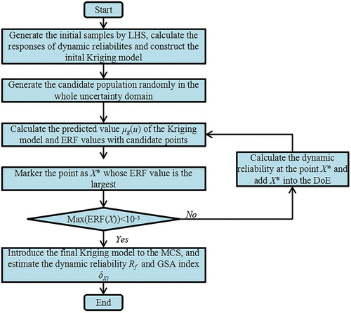
4.3. Solution process of ALK

Step 1. Generate initial samples $X_t=\left(X_{1,t},X_{2,t},\cdots ,X_{n,t}\right)\left(t=1,2,\cdots ,N_x\right)$ randomly by Latin hypercube sampling (LHS) method in the uncertainty domain, calculate the values of dynamic reliabilities and construct the initial Kriging model. Here, $N=12$.

Step 2. Generate a large number of candidate samples to prepare for the selection of ERF. In order to fill the uncertainty domain with candidate samples, the number of candidate points is taken as $N_c={10}^5$.

Step 3. Calculate the predicted value ${\mu }_g\left(X\right)$ of the Kriging model as well as ERF values of candidate points, and mark the point as $X^{\ast }$ whose ERF value is the largest.

Step 4. If the maximum value of ERF satisfies the threshold of convergence condition, then transfer to Step 6. The threshold in this paper is ${10}^{-3}$.

Step 5. If the convergence condition in Step 4 cannot be satisfied, add $X^{\ast }$ to the DoE and calculate the value of dynamic reliability at the point of $X^{\ast }$. Then return to Step 3.

Step 6. Based on the Kriging established finally, introduce it into the Monte Carlo method to solve the dynamic reliability and GSA index of the structure or system.

The solution process flowchart is shown in Figure 1.

Figure 1. The flowchart of the ALK method.

5. Examples

5.1. Simply supported bar

Considering a simply supported bar, a stationary random excitation is applied to the ends of the bar. The $m$, $k$ and $c$ are mass, stiffness and damping of the bar, respectively. This example contains 3 input random variables, i.e. $m$, $k$ and $c$, which obey normal distribution and are independent with each other. The means of them are $15$, $40$ and $0.05$ while the coefficient of variation $\nu$ is the same as 0.05. The random excitation is a stationary random process, whose auto-spectrum is constant $S_{ff}\left(\omega \right)=S_0=1$, setting $\omega =\left[0,10\right]$. The constant $b$ in equation (1) is set as $2$ in this paper. The variable $t$ is set as $100s$.

Considering two conditions: $\nu =0.1$ and $\nu =0.2$. The dynamic reliabilities of bar calculated by MCS method and ALK method are shown in Table 1 while the sample number of matrix $\mathbf{A}$ and $\mathbf{B}$ is $N_1=N_2=1000$. The Figure 2 illustrates the relationship between the sampling frequency and the results in the MCS method. The results in Table 1 demonstrate that the ALK method only needs dozens of performance function evaluation to obtain the dynamic reliability with slight errors while the MCS method need call the performance function tens of thousands of times. The ALK method has extremely high computational efficiency. The curves in Figure 2 further illustrate that the MCS method requires a lot of samples to guarantee the stability of the results. On the contrast, the ALK method just needs 35 iterative simulations to get accurate results. The Figure 3 shows the maximum ERF values of the training points of iteration and the Figure 4 shows the true values of the $R(t{)}_{\mathit{X}}$ of the training points in the ALK method. Both of Figure 3 and 4 indicate that the convergence rate of the ALK method is very high in the iterative history which further demonstrates the efficiency of the ALK method.

Figure 2. The dynamic reliabilities with different sample numbers calculated by MCS method.

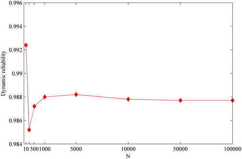
Figure 3. The maximum ERF values at the training points by ALK method in iteration history ($\nu =0.2$).

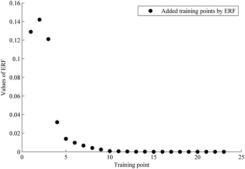
Figure 4. The true values of training points by ALK method in iteration history ($\nu =0.2$).

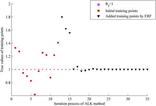
Table 1. The dynamic reliabilities of the bar under two conditions.

	MCS	ALK	Error
$R_t\left(\nu =0.1\right)$	0.9878^(10000)	0.9795^(28)	0.84%
$R_t\left(\nu =0.2\right)$	0.9494^(10000)	0.9458^(35)	0.38%

Note: The numbers in brackets indicate the times of performance function evaluation

The results of moment-independent GSA calculated by ALK and MCS method are shown in Figure 5. It can be seen that the importance ranking of input variables is $m>k>c$ which indicates that $m$ has the largest effect on the dynamic reliability of the bar under stochastic excitation while $c$ has the smallest effect. To guarantee the security of the bar and improve the dynamic reliability, researchers and designers should strictly control the uncertainty of $m$. 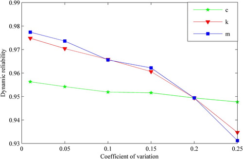In the meanwhile, the importance rankings of variables obtained by ALK method and MCS method are coincident and the GSA index values of input variables are basically coincident. The Figure 6 shows the variation of dynamic reliabilities with different coefficients of variation of random variables. It demonstrates the validity of the results of importance ranking obtained from GSA. With the coefficient of variation increasing, the dynamic reliabilities reduce most caused by the varying of $m$, followed by $k$ and $c$.

Figure 5. The GSA indices of variables of bar by MCS and ALK methods.

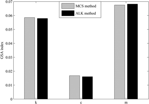
Figure 6. The dynamic reliabilities with different coefficients of variation.

5.2. 16-bar structure

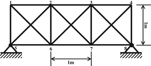
As shown in Figure 7, the dynamic reliability of a 16-bar structure is analyzed in this part. The cross section of each bars is square and the length of side is $a=0.1m$. The length of all of the horizontal and vertical bars is $L$. The Young’ modulus and mass density are $E$ and $\rho$, respectively. There are 3 input random variables, i.e. $L$, $E$ and $\rho$, and the distribution type of them is Gaussian distribution. The mean values of variables are respectively $1.0m$, $300GPa$ and $7800kg/\phantom{7800kg{m}^3}{m}^3$, while the coefficient of variation of variables is taken as 0.05. Load random white noise excitation at the left fixed end. The spectral value is $0.1g^2/\phantom{g^{2}Hz}Hz$ and the effective frequency band is $f\in \left[0,150\right]Hz$. The direction of excitation is the positive direction of y axis. The damping coefficient of structure is 0.02. Calculate the dynamic reliability of the 16-bar structure with MCS method and ALK method, respectively.

Figure 7. The schematic diagram of 16-bar structure.

Considering two conditions: $t=900s$ and $t=1000s$. The dynamic reliabilities of 16-bar structure under two conditions have been listed in Table 2. It can be seen that the dynamic reliabilities are $R_f^{t=900}=0.9410$ and $R_f^{t=1000}=0.9353$ by MCS method. The reliabilities calculated by ALK method just have slight error compared with those obtained by MCS method, but the times of performance function evaluation of ALK method are much less than those of MCS method.

Table 2. The dynamic reliabilities of 16-bar structure with different $t$_.

	MCS	ALK	Error
$R_t\left(t=900\right)$	0.9410^(10000)	0.9444^(35)	0.36%
$R_t\left(t=1000\right)$	0.9353^(10000)	0.9393^(37)	0.43%

Note: The numbers in brackets indicate the times of performance function evaluation

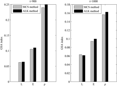
The GSA indices of input variables on the dynamic reliability calculated by MCS and ALK methods are shown in Figure 8. The importance ranking of variables obtained by these two methods is same and it is $\rho >E>L$, which indicates that the variable $\rho$ affects the dynamic reliability of the 16-bar structure most while the variable $L$ affects least. It means that we should focus on the information collection of important variables $\rho$ and $E$ which have large effect on the dynamic output in the dynamic reliability design and optimization of the 16-bar structure. This can reduce the level of uncertainty of structure dynamic reliability furthest. In addition, according to the importance ranking of random variables, the random variables with higher importance degree should be thought about first in the dynamic reliability design of the 16-bar structure to improve the reliability of the structure. Meanwhile, some variables with low importance degree could be ignored to reduce the dimensionality to simplify the analysis process in the dynamic reliability design of the 16-bar structure. On the other hand, comparing the dynamic reliabilities and GSA index values of the 16-bar structure at $t=900s$ and $t=1000s$, it can be seen that both of the reliabilities and GSA indices decrease with the extension of time.

Figure 8. The GSA indices of variables of 16-bar structure by MCS and ALK methods.

5.3. Hydraulic pipe

Consider a hydraulic pipe model as shown in Figure 9 whose material is stainless steel 1Cr18Ni9Ti. The Poisson ratio, elastic modulus, diameter, thickness, fluid density and the internal pressure are ${\nu }_p=0.3$, ${\rho }_P=7800kg/\phantom{7800kg{m}^3}{m}^3$, $E=184GPa$, $d=12mm$, $h=1mm$, ${\rho }_F=1000kg/\phantom{1000kg{m}^3}{m}^3$ and $P=21MPa$. We assume that the axial direction of the long pipe coincides with x axis and the axial direction of vertical pipe coincides with y axis. The supports only restrain the radial displacement of the pipe, i.e. the direction of x axis, while the displacements of axial direction (the direction of y axis) and rotate direction are free. The support stiffness is assumed as $K=0.5E^{7}N/\phantom{Nm}m$. The transfer coefficient of the clamps is $0.5$. The input random variables of hydraulic pipe structure are listed in Table 3, where the $L$ and $H$ indicate the locations of Clamp 1 and Clamp 2, i.e. the $L$ is the length from the fixed end to the Clamp 1 and the $H$ is the length from the curved cube to the Clamp 2.

Figure 9. The schematic diagram of air pipe with random variation excitations.

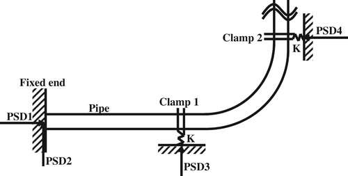
Table 3. The input random variables of air pipe.

Input variables(unit)	Distribution type	Mean	Coefficient of variation
${\rho }_p\left(Kg/\phantom{Kg{m}^3}\right)$	Normal	7800	0.01
$E\left(GPa\right)$	Normal	184	0.01
$L\left(m\right)$	Normal	0.21	0.01
$H\left(m\right)$	Normal	0.042	0.01

In stochastic vibration analysis, base stochastic excitation is transferred through the fixed support and clamps. The base indicates the interfaces jointing with pipe system. The interfaces and pipe are restrained together with fixed support and clamps. The vibration of airframe transfers to pipe structure through fixed support and clamps. Therefore, the stochastic excitations are loaded to these fixed support and clamps.

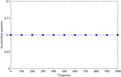
The vibrational white noise spectrum is adopted as the random load, whose frequency range is from 0.1 Hz to 1000 Hz and the spectral value is $0.1$. The excited directions are shown in Figure 9. The frequency-acceleration spectrum of power spectral density (PSD) is shown in Figure 10.

Figure 10. The acceleration spectrum of PSD.

The dynamic reliabilities and GSA indices calculated by MCS and ALK methods are shown in Table 4. The results calculated by ALK method just have slight errors compared with those calculated by MCS method. But the times of performance function evaluation of ALK method is only 67 which is much less than $4\times {10}^4$ calls of performance function of MCS method. It should be noted that the sample number of MCS method is $N_1=N_2=10000$. It fully demonstrates the efficiency and accuracy of ALK method in engineering practice. The Figure 11 shows the GSA indices and the importance ranking of the input random variables, which is $E>{\rho }_p>H>L$. It proves that the uncertainty of $E$ has the largest effect on the dynamic reliability of the hydraulic pipe followed by ${\rho }_p$ while the uncertainty of $L$ has the least effect on the dynamic reliability. So the dynamic reliability of the hydraulic pipe can be strengthened furthest by reducing the uncertainty of $E$, followed by ${\rho }_p$, $H$ and $L$. In the dynamic reliability design and optimization of hydraulic pipe, the variables with high importance degree should be taken into account at first and the variables with low importance degree even nearly to zero, such as the GSA value of $L$, could be neglected to reduce the dimensionality. The importance ranking provides significant guidance and reference for the dynamic reliability design of the hydraulic pipe system.

Figure 11. The GSA indices of variables of air pipe by MCS and ALK methods.

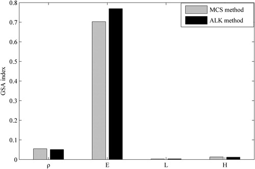
Table 4. The dynamic reliabilities and GSA indices of air pipe.

	$R_f$	${\delta }_{{\rho }_p}$	${\delta }_E$	${\delta }_L$	${\delta }_H$	Times of function evaluation
MCS	0.9692	0.0548	0.703	0.0031	0.0128	40000
ALK	0.9682	0.0511	0.769	0.0032	0.0120	67
Error	0.10%	6.81%	9.41%	5.47%	7.08%

In addition, comparing with the $4\times {10}^4$ calls of performance function of MCS method, the ALK method only selects 67 points to establish the final Kriging model for calculating the dynamic reliability and GSA index, with 12 points to establish the initial Kriging model and 55 points selected by ERF iterative process. The ALK method reduces the computational cost greatly. At the same time, the ALK method has a fine performance on the convergence rate.

6. Conclusion

This paper proposes a dynamic reliability and global sensitivity analysis method of double random vibration system based on the active learning Kriging model. A dynamic reliability analysis model based on the Miner criterion for the double random vibration system is established. Furthermore, a moment-independent GSA index to the dynamic reliability is proposed. Meanwhile, an ALK method is introduced to calculate the dynamic reliability and GSA index of double random vibration problems.

Three examples demonstrate the feasibility, necessity and efficiency of the proposed method. The results demonstrate that the moment-independent GSA index can effectively measure the effect of input random variables on the dynamic reliability of double random vibration system, providing significant guidance and reference for the dynamic reliability design and optimization of double random vibration system. Researchers can mainly consider the input variables with high GSA indices and neglect the input variables with low GSA indices which are even close to zero. It indicates the direction for improving the dynamic reliability of double random vibration system. In the meanwhile, the ALK method introduced in this paper shows high efficiency and great accuracy compared with MCS method, which is essential for the practical application in engineering of the proposed method in this paper.

Acknowledgements

The authors received no financial support for the research, authorship, and/or publication of this article.

Disclosure statement

No potential conflict of interest was reported by the author(s).

References

- Yan Z, Pan X, Lin JH. Double random vibration analysis for coupled Vehicle-Track systems with parameter uncertainties. In: International Conference on vulnerability and risk analysis and management. Liverpool; 2014 July. p. 456–464.
- Sofi A, Romeo E. A unified response surface framework for the interval and stochastic finite element analysis of structures with uncertain parameters. Probab Eng Mech. 2018;54:25–36.
- Schenk CA, Pradlwarter HJ, Schueller GI. On the dynamic stochastic response of FE models. Probab Eng Mech. 2004;19(1-2):161–170.
- Wang W, Zhang YM, Li CY. Dynamic reliability nanlysis of linear guides in positioning precision. Mech Mach Theory. 2017;116:451–464.
- Lu C, Feng YW, Liem RP, et al. Improved Kriging with extremum response surface method for structural dynamic reliability and sensitivity analyses. Aerosp Sci Technol. 2018;76:164–175.
- Babykina G, Brinze NI, Aubry JF. Modeling and simulation of a controlled steam generator in the context of dynamic reliability using a stochastic hybrid automaton. Reliab Eng Syst Saf. 2016;152:115–116.
- Chen JB, Li J. The extreme value distribution and dynamic reliability analysis of nonlinear structures with uncertain parameters. Struct Saf. 2007;29(2):77–93.
- Du WQ, Luo YX, Wang YQ. A time-variant performance measure approach for dynamic reliability based design optimization. Appl Math Model. 2019;76:71–86.
- Gao HF, Zio E, Guo JJ, et al. Dynamic probabilistic-based LCF damage assessment of turbine blades regarding time-varying multi-physical field loads. Eng Fail Anal. 2020;108:104193.
- Hu HQ, Huang Y. A dynamic reliability approach to seismic vulnerability analysis of earth dams. Geomech Eng. 2019;18(6):661–668.
- Yang C, Lu ZX, Yang ZY, et al. Parameter identification for structural dynamics based on interval analysis algorithm. Acta Astronaut. 2018;145:131–140.
- Yang C, Lu ZX, Yang ZY. Robust optimal sensor placement for uncertain structures with interval parameters. IEEE Sens J. 2018;18(5):2031–2041.
- Wu YT, Mohanty SJ. Variable screening and ranking using sampling-based sensitivity measures. Reliab Eng Syst Saf. 2006;91:634–647.
- Lu ZZ, Song J, Song SF, et al. Reliability sensitivity by method of moments. Appl Math Model. 2010;34(10):2860–2871.
- Liu J, Tu LW, Liu GZ, et al. An analytical structural global sensitivity analysis method based on direct integral. Inverse Probl Sci Eng. 2019;27(11):1559–1576.
- Helton JC, Davi FJ. Latin hypercube sampling and the propagation of uncertainty in analysis of complex systems. Reliab Eng Syst Saf. 2003;81(1):23–69.
- Helton JC, Johnson JD, Sallaberry CJ, et al. Survey of sampling-based methods for uncertainty and sensitivity analysis. Reliab Eng Syst Saf. 2006;91(10):1175–1209.
- Wei PF, Lu ZZ, Song JW. A new variance-based global sensitivity analysis technique. Comput Phys Comm. 2013;184:2540–2551.
- Wei PF, Lu ZZ, Song JW. Regional and parametric sensitivity analysis of Sobol’s indices. Reliab Eng Syst Saf. 2015;137:87–100.
- Cui L, Lu ZZ, Zhao X. Moment-independent importance measure of basic random variable and its probability density evolution solution. Sci China Tech Sci. 2010;53(4):1138–1145.
- Borgonovo E, Castaings W, Tarantola S. Moment independent importance measures: new results and analytical test cases. Risk Anal. 2011;31(3):404–428.
- Liu Q, Homma T. A new computational method of a moment-independent uncertainty importance measure. Reliab Eng Syst Saf. 2009;94(7):1205–1211.
- Maschio C, Denis JS. A new methodology for Bayesian history matching using parallel interacting Markov chain Monte Carlo. Inverse Probl Sci Eng. 2018;26(4):498–529.
- Hasofer AM, Lind NC. An exact and invariant first order reliability format. J Eng Mech Div. 1974;100:111–121.
- Zhao YG, Ono T. A general procedure for first/second-order reliability method (FORM/SORM). Struct Saf. 1999;21(2):95–112.
- Meng Z, Zhou HL, Li G, et al. A hybrid sequential approximate programming method for second-order reliability-based design optimization approach. Acta Mech. 2017;228(5):1–14.
- Bichon BJ, Eldred MS, Swiler LP, et al. Efficient global reliability analysis for nonlinear implicit performance functions. AIAA J. 2008;46(10):2459–2468.
- Bichon BJ, Mcfarland JM, Welch WJ. Efficient surrogate models for reliability analysis of systems with multiple failure modes. Reliab Eng Syst Saf. 2011;96(10):1386–1395.
- Echard B, Gayton N, Lemarie M. AK-MCS: An active learning reliability method combining Kriging and Monte Carlo simulation. Struct Saf. 2011;33(2):145–154.
- Yang XF, Liu YS, Zhang YS, et al. An active learning Kriging model for hybrid reliability analysis with both random and interval variables. Struct Multidisc Optim. 2015;51(5):1003–1016.
- Yang XF, Liu YS, Zhang YS, et al. Hybrid reliability analysis with both random and probability-box variables. Acta Mech. 2015;226(5):1341–1357.
- Huang X, Chen J, Zhu H. Assessing small failure probabilities by AK-SS: an active learning method combining Kriging and subset simulation. Struct Saf. 2016;59:86–95.
- Zhang YS, Liu YS, Yang XF. Parametric sensitivity analysis for importance measure on failure probability and its efficient Kriging solution. Math Probl Eng. 2015;2015:1–130.
- Dubourg V, Sudret B. Meta-model-based importance sampling for reliability sensitivity analysis. Struct Saf. 2014;49:27–36.
- Song LK, Bai GC, Fei CW. Dynamic surrogate modeling approach for probabilistic creep-fatigue life evaluation of turbine disks. Aerosp Sci Technol. 2019;95:105439.
- Li Y, Barkey LME, Kang HT. Metal fatigue analysis handbook: practical problem-solving techniques for computer-aided engineering. 2011.
- Li GQ, Cao H, Li QS, et al. Structural dynamic reliability theory and its application. Beijing: Seismological Press, in Chinese; 1993.
- Zhao YG, One T, Idota H. Response uncertainty and time-variant reliability analysis for hysteretic MDF structures. Earthq Eng Struct Dyn. 1999;28:1187–1213.
- Borgonovo E. A new uncertainty importance measure. Reliab Eng Syst Saf. 2007;92(6):771–784.
- Liu QF, Zeng JP, Yang G. MrDIRECT: a multilevel robust DIRECT algorithm for global optimization problems. J Glob Optim. 2015;62(2):205–227.