Effective grain orientation mapping of complex and locally anisotropic media for improved imaging in ultrasonic non-destructive testing

Abstract

Imaging defects in austenitic welds presents a significant challenge for the ultrasonic non-destructive testing community. Due to the heating process during their manufacture, a dendritic structure develops, exhibiting large grains with locally anisotropic properties which cause the ultrasonic waves to scatter and refract. When basic imaging algorithms, which typically make constant wave speed assumptions, are applied to datasets arising from the inspection of these welds, the resulting defect reconstructions are often distorted and difficult to interpret correctly. However, knowledge of the underlying spatially varying material properties allows correction of the expected wave travel times and thus results in more reliable defect reconstructions. In this paper, an approximation to the underlying, locally anisotropic structure of the weld is constructed from ultrasonic time of flight data. A new forward model of wave front propagation in locally anisotropic media is presented and used within the reversible-jump Markov chain Monte Carlo method to invert for the map of effective grain orientations across different regions of the weld. This forward model and estimated map are then used as the basis for an advanced imaging algorithm and the resulting defect reconstructions exhibit a significant improvement across multiple flaw characterization metrics.

Keywords:

• Imaging
• wave propagation
• nondestructive evaluation
• ultrasonics
• Bayesian inverse problems

2010 Mathematics Subject Classifications:

• 00
• 60

1. Introduction

In many countries, infrastructure is ageing and cannot be replaced due to global financial pressures. Industry is therefore presented with the challenging problem of safely maintaining their infrastructure and extending its life span. Ultrasonic non-destructive testing (NDT) involves the transmission of mechanical waves through industrial components to facilitate the detection of interior damage and offers an economically and environmentally desirable solution to this challenge. Networks of ultrasonic transducers, typically arranged in linear arrays, are deployed to carry out these inspections, resulting in large volumes of often noisy data. This data can be acquired using the Full Matrix Capture (FMC) technique [1], where each array element fires sequentially whilst all of the array elements record the reflected data simultaneously, thus maximizing the information extracted from a single array position. Using mathematical algorithms to decipher the resulting data sets, an image of the component's interior can be constructed and, in scenarios where the component is composed of a homogeneous material, defects can be reliably detected and characterized [1,2]. However, when the material exhibits inhomogeneous and/or anisotropic behaviour, its inspection becomes challenging [3–5]: the ultrasonic wave paths are distorted and their expected arrival times (on which many existing imaging algorithms are based) are usually no longer reliable.

One particularly challenging example of this behaviour occurs in austenitic steel welds [6–9]. These welds are popular within heavy industry due to their strength and corrosion resistance. However, due to the heating process during their manufacture, crystals undergo epitaxial growth where their primary axis aligns with the direction of heat flow, creating a locally anisotropic microstructure. When traditional NDT imaging algorithms (which assume a constant, isotropic velocity throughout the medium) are applied to data sets arising from such components, the resulting images typically display poorly characterized and mislocated flaws. Furthermore, with the introduction of additive manufacturing methods and industry's increasing reliance on strong, durable composite materials which are heterogeneous by design, it is becoming increasingly important to address the problem of imaging defects embedded in complex media.

It has already been shown that a priori knowledge of a material's spatially variant properties can be used to construct more accurate and reliable images of embedded defects [3–5]. Although the microstructural maps required for this correction can be obtained experimentally [6,10], such techniques are not considered to be strictly non-destructive and thus cannot be deployed in situ. However, these techniques have provided invaluable insight into the structure and crystallography of these materials, as have the models of wave propagation in complex media presented in [11–14].

The inverse problem of recovering information about the spatially varying material properties of a component from ultrasonic phased array data has yet to be solved satisfactorily, and is attracting increased attention within the NDT community. In recent years, some work has been carried out on the determination of crystallographic orientation in single crystal materials [15] and mapping the velocity field in locally isotropic random media [5]. In the case of locally anisotropic polycrystalline materials (for example, steel welds [4,8,16]), the wave speed through the material is dependent on the angle of incidence of the wave, and so a single map of the velocity field cannot fully represent the complexity of the wave's journey. Thus, grain orientation maps are required, where small regions are assigned a single orientation representing the dominant orientation of the aggregated crystals at that point in the domain. This aggregation process has previously been studied across different length scales: in [9,17] macro regions are considered; in [6,18] grain-size regions are studied and in [19] an intermediate regime of averaging is examined.

In the last 20 years, much work on obtaining these orientation or stiffness maps has been conducted. The Modelling anIsotropy from Notebook of Arc welding (MINA) model was first presented in [19]. Given a small set of welding parameters, it was shown that the MINA model could predict the variation in local anisotropy that is present in a multipass weld. This work was validated against experimental EBSD measurements in [20] and built upon in [8,16], where ultrasonic phased array measurements were used to invert for the key welding parameters in the case where these are not known. Further examination of the orientation maps specific to welds is carried out in [17] where the weld structure is studied using a combination of finite element modelling and metallographic and crystallographic analyses and the elastic constants are also inverted from ultrasonic measurements. A more generally applicable approach is studied in [4] where ultrasonic phased array travel time data is inverted using a Markov chain Monte Carlo approach to reconstruct the orientations map of an austenitic steel weld. Here, the authors initialized the algorithm using an approximation of the weld structure generated using the Ogilvy model of a weld [21].

Building upon this existing body of work, the work presented in this paper presents the reversible-jump Markov chain Monte Carlo (rj-MCMC) method [22] as an alternative means for inverting ultrasonic phased array data to obtain information on the distribution of crystal orientations in polycrystalline materials. The authors have already applied this inversion method to reconstruct the varying velocity field in locally isotropic, random media [5,23,24] and in this paper, the method is extended to map the locally anisotropic grain structure of austenitic steel welds. Similar to the methodology presented in [4], and in contrast to the work carried out in [8,16,17,19,20], this methodology is not weld-specific and may be applied to any environment in which waves propagate through heterogeneous and locally anisotropic media (for example, it may be easily adapted for application by the seismic community where isotropic assumptions are often made in materials known to be anisotropic, negatively impacting the fidelity of the resulting reconstructions). Furthermore, we employ a Bayesian approach rather than a deterministic one, which provides additional information on the reconstructed maps; most notably the standard deviation map which highlights regions that lie at the interface between different macro regions of the materials. Additionally, and unlike the work presented in [4], no a priori assumptions are made on the distribution of crystal orientations within the component here: the initial model arbitrarily assigns orientations drawn from an uninformative uniform distribution to the irregularly partitioned domain, to retain the general nature of the approach and to avoid the inclusion of any bias. The only prior information exploited is the sample's exterior dimensions, the location of the transmitting and receiving array elements and the material's slowness curve (derived from the elastic constants which we assume are known here but which in practice may need to be approximated experimentally and the uncertainty attached to these approximations considered [17,25]). Note we consider only longitudinal waves travelling in the plane transverse to the weld direction as it has been shown from experimental measurements in flat welds that the beam skewing out of the weld is weak and thus we can approximate the weld as transversely isotropic [17,20]. The results presented are complementary to those that have gone before as they offer an alternative approximation to the weld geometry. This is driven by the irregular partitioning of the domain in contrast to the regular square mesh used in the previous studies. Since the rj-MCMC is transdimensional (that is the number of degrees of freedom in partitioning the domain can change) and naturally parsimonious, the resulting reconstructions are often much coarser than those obtained in [4,19], for example, exhibiting macro trends in the distribution of anisotropy and offering an alternative perspective on the weld structure. It is due to this macroscale perspective that we refrain here from using the term microstructure and instead refer to effective orientation maps. This paper also contributes a novel forward model of wave front propagation through the anisotropic medium; the anisotropic multi-stencil fast marching method (AMSFMM). In contrast to Dijkstra's method, which is implemented in [4] and does not converge to the underlying partial differential equation for travel time, it has been shown that the higher order fast marching method (on which the AMSFM is based on) diminishes the grid bias and converges to the underlying geodesic distance when the grid step size tends to zero [26]. Once the orientation map has been constructed (using the rj-MCMC), the AMSFMM is used again in conjunction with the Total Focussing Method (TFM) [1] (from herein we refer to this extension as the TFM+) to correct for fluctuations in the predicted travel times of each wave caused by the anisotropic nature of the material. The success of the approach is quantified via the accuracy of the resulting flaw image and how it compares to that arising from application of the standard TFM algorithm (which assumes a constant wave speed throughout the domain) in terms of defect characterization and positioning.

2. Methodology

2.1. The observed data

Ultrasonic phased array systems have become increasingly popular as tools for flaw detection and characterization within the non-destructive testing industry. They provide improved resolution and coverage by transmitting and receiving ultrasound signals over multiple transducers, which, when fired in predefined sequences, can provide increased control over beam directivity [27]. The capability of these arrays to both transmit and receive ultrasonic signals simultaneously presents us with two alternative experimental set-up options: the pulse-echo set-up, where only one phased array is employed to simultaneously transmit and receive signals, and the pitch-catch arrangement, where two phased arrays are employed, one to transmit and one to receive. In both cases, when the full matrix capture (FMC) technique is employed to collect the data [1] we have N transmitting elements and N receiving elements, and thus $N^2$ so-called A-scans (the collected time-series data). However, for the work presented in this paper, we need only the first time of arrival of the wave, and do not exploit the entirety of the reflected waveform as is the practice in the computationally expensive full waveform inversion techniques [28,29]. Additionally, we consider only a pitch-catch scenario, where two arrays are placed directly opposite each other, on either side of the component (known as through-transmission). This set up simplifies the extraction of the first time of arrival of the signal: in the pulse-echo arrangement, scattering by other artefacts can interfere with the detection of the back wall scattering and an added element of uncertainty is thus introduced. In the pitch-catch scenario, the time of flight is estimated by the first point in time that $A_{s,r}(t)>\epsilon$, where A is the time domain signal transmitted at element s and received at element r, ϵ is some chosen amplitude threshold (${10}^{-6}$Pa here), and $0\le t\le T$ is the time period over which the signal is collected. Of course, in this simulated environment, there is some uncertainty attached to the selection of arrival time threshold ϵ, and this uncertainty would be amplified in the extraction of time of flight data in an experimental scenario. However, the chosen inversion methodology also inverts for the system noise level, a global parameter which aggregates the aleatoric and epistemic uncertainties, thus tempering the impact of uncertainty in the travel time estimations. Once the arrival times have been obtained, they are stored in a time of flight (ToF) matrix $T_0$, where each element $t_{s,r}$ represents the time taken for the wave to travel from transmitting element s to receiving element r. In a homogeneous, globally isotropic medium, the time taken is dependent only on distance and so we obtain symmetric, banded ToF matrices. However, as soon as an element of heterogeneity is introduced, these bands are distorted [5] and it is this distortion that we exploit to obtain information on the material's underlying structure.

2.2. Material parametrization by Voronoi diagrams

To minimize the degrees of freedom within our inverse problem, we reconstruct a lower resolution map of the grain orientation maps than that afforded by electron backscatter diffraction measurements, for example. To this end, groups of crystallites are considered as a single homogeneous grain which is assigned an effective orientation, thus producing a coarsened representation of the material's spatially varying structure. In this paper, we restrict our attention to polycrystalline materials, whose grains are irregularly shaped and cannot be well described by a coarse rectangular grid. Voronoi diagrams have already been used successfully as the basis for finite element (FE) simulations of waves propagating through polycrystalline materials [18,30]. Given an arbitrary set of seeds S (here a set of two-dimensional Cartesian coordinates), a Voronoi tessellation can be generated by first constructing the Delauney triangulation of these points and then taking the perpendicular bisectors of its edges to be the edges of the Voronoi diagram (the Voronoi diagram is the geometric dual of the Delauney triangulation) [31]. Thus, the Voronoi diagram is a set of non-overlapping convex regions or cells where any point within a cell is closer to the seed of that cell than any other seed. These seeds are a discrete set of points $(x_i,y_i)$ for $i=1,\dots ,M$, where M is the number of regions and so the Voronoi diagram describes the partitioning of our spatial domain using $2M$ variables.

To parameterize the weld with a Voronoi diagram, we must assign a third parameter to each cell: its orientation ${\varphi }_i$. In this work, we consider only in plane rotation and so the assigned orientation dictates the rotation of a slowness curve in each cell (as opposed to a slowness surface). Thus, given the incident wave angle, the speed that the wave travels through that cell can be calculated from where the wave vector bisects the rotated slowness curve. The longitudinal group slowness curve (the reciprocal of the group velocity) for a transversely isotropic cubic austenitic weld is obtained by solving the Christoffel equation [12] with a cubic stiffness tensor where $c_{11}=203.6$GPa, $c_{12}=133.5$GPa and $c_{44}=129.8$GPa and the density is $\rho =7874$kg/$m^3$ (these are taken from the weld properties used in [32,33]). Note that the method is not restricted to the examination of cubic materials and a straightforward extension could be realized to consider hexagonal materials. Thus, we have a parametrization with 3M + 1 unknowns (where M is itself an unknown), and $N^2$ equations, describing the known time of arrival between every transmit/receive pair of elements.

2.3. The anisotropic multi-Stencil fast Marching method

Having parametrized the material's structure using Voronoi cells, we now require an efficient forward model which outputs the time of flight matrix $T_m$ for any particular instance of the material model m. To consider the effects of the locally anisotropic grain structure on the wave's path and speed, we have developed a new algorithm based on the fast marching method (FMM) [34], to model the monotonically advancing wave front through the material. In the standard FMM, we let $\tau (x_i,y_j,s)$ denote the shortest time for a wave to travel from the transmitter $s\in \mathrm{\partial }I$, on the boundary of the discretized representation of our image domain $I=x\times y$, to the point $(x_i,y_j)\in I$. The Eikonal equation, $|\mathrm{\nabla }\tau (x_i,y_j,s)|=1/V(x_i,y_j)$, is then solved for $\tau (x_i,y_j,s)$ using an upwind finite difference scheme [34,35], where, $V(x_i,y_j)$ represents the velocity at point $(x_i,y_j)$. 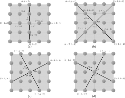Solving this over a regular grid superimposed over a given velocity field, the shortest travel-time between each transmitter s and receiver $r\in \mathrm{\partial }I$ can be calculated and the matrix $T_m$ constructed (note that only the travel time information is modelled and other physical phenomena such as scattering, attenuation and dispersion are ignored). To consider maps of the spatially varying crystal orientation rather than the inhomogeneous velocity field, the algorithm requires some modification. Firstly, in the implementation of the standard FMM, movement of the wave is restricted along the vertical and horizontal edges of a regular rectangular mesh. This limitation means that even if the wave speed at each point on the grid is calculated by taking into account the wave direction and the rotation of the slowness curve at that point, the cell is still treated as locally isotropic due to the symmetries of the slowness curve [36]. To counter this, we first exploit the multi-stencils fast marching method (MSFM) [37]. It is well known that errors accumulate along diagonal trajectories when the fast marching method is employed as it considers only nearest neighbours of each node. The MSFM (in two dimensions) introduces an additional stencil at each node, rotated by ${45}^{\circ }$, allowing next nearest neighbours (neighbouring nodes along the diagonal) to contribute to the shortest time calculations at each point. This significantly improves the error in travel time estimation along the diagonal directions and is sufficient for the study of wave propagation in locally isotropic media [5]. However, due to the additional diagonal axes of symmetry of our slowness curve, to account for local anisotropy, we must extend this principle and examine four stencils (denoted ${\mathcal{S}}_H$, H = 1, 2, 3, 4) on a 25 point finite difference scheme (see Figure 1), allowing movement of the wave along four distinct directions in each quadrant.This requires use of a mixed order scheme, where calculations on ${\mathcal{S}}_1$ and ${\mathcal{S}}_2$ are nominally second order accurate (reverting to a first-order approximation when the travel-times for the second-order approximation are unavailable) and the solutions found on stencils ${\mathcal{S}}_3$ and ${\mathcal{S}}_4$ are only first order accurate and solved on a coarser grid. This mixed order, four stencil approach combined with the assignment of an orientation to each cell rather than wave speed, forms the basis for our anisotropic multi-stencil fast marching method (AMSFMM). Importantly, we propose that the Eikonal equation can be solved locally for each of the four stencils in the same manner as employed by the standard FMM by assigning a velocity at each node that is dependent on the angle of rotation of the stencil along which it is being solved and the assigned crystal orientation at that node. Thus, locally, the solver treats the medium as isotropic but in actual fact the incident wave direction and locally anisotropic crystal orientation have already been accounted for. To begin, we rewrite the Eikonal equation as (1) $|\mathrm{\nabla }\tau (x_i,y_j,s))|=\hat{V}({\varphi }_{i,j},{\mathcal{S}}_H)$(1) where $\hat{V}({\varphi }_{i,j},{\mathcal{S}}_H)$ is the slowness at the point $(x_i,y_j)$ dependent on the crystal orientation ${\varphi }_{i,j}$ assigned to that point and the rotation of the stencil ${\mathcal{S}}_H$ along which the equation is being solved. When evaluating over ${\mathcal{S}}_1$, we adopt the second order forward and backward finite difference approximations of the gradient to approximate Equation (1(1) $|\mathrm{\nabla }\tau (x_i,y_j,s))|=\hat{V}({\varphi }_{i,j},{\mathcal{S}}_H)$(1) ) by (2) $\sum _{v=1}^{2}max{(\frac{3}{2{\mathrm{\Delta }}_v}({\tau }_{i,j}-{\tau }_v),0)}^2=\hat{V}({\varphi }_{i,j},{\mathcal{S}}_H{)}^2$(2) where ${\tau }_{i,j}=\tau (x_i,y_j,s)$, here ${\mathrm{\Delta }}_1={\mathrm{\Delta }}_x$ is the grid side length in the x direction and ${\mathrm{\Delta }}_2={\mathrm{\Delta }}_y$ is the grid side length in the y direction, ${\tau }_1=min(\frac{4{\tau }_{i-1,j}-{\tau }_{i-2,j}}{3},\frac{4{\tau }_{i+1,j}-{\tau }_{i+2,j}}{3})$ and ${\tau }_2=min(\frac{4{\tau }_{i,j-1}-{\tau }_{i,j-2}}{3},\frac{4{\tau }_{i,j+1}-{\tau }_{i,j+2}}{3})$. If the solution (${\tau }_{i,j}^{\ast }$, say) to Equation (2(2) $\sum _{v=1}^{2}max{(\frac{3}{2{\mathrm{\Delta }}_v}({\tau }_{i,j}-{\tau }_v),0)}^2=\hat{V}({\varphi }_{i,j},{\mathcal{S}}_H{)}^2$(2) ) is greater than $max({\tau }_1,{\tau }_2)$, then ${\tau }_{i,j}$ is the solution of the quadratic equation (3) $\sum _{v=1}^2{(\frac{3}{2{\mathrm{\Delta }}_v}({\tau }_{i,j}-{\tau }_v))}^2=\hat{V}({\varphi }_{i,j},{\mathcal{S}}_H{)}^2.$(3) Otherwise, if ${\tau }_1>{\tau }_{i,j}^{\ast }>{\tau }_2$ then ${\tau }_{i,j}={\tau }_2+{\mathrm{\Delta }}_2\hat{V}({\varphi }_{i,j},{\mathcal{S}}_H)$, or if ${\tau }_2>{\tau }_{i,j}^{\ast }>{\tau }_1$ then ${\tau }_{i,j}={\tau }_1+{\mathrm{\Delta }}_1\hat{V}({\varphi }_{i,j},{\mathcal{S}}_H)$. On ${\mathcal{S}}_1$, this is simply the the Higher Accuracy Fast Marching Method [37]. To adopt our multi-stencil approach, we enforce the condition that ${\mathrm{\Delta }}_x={\mathrm{\Delta }}_y$ so that we are operating on a regular square mesh. On stencil ${\mathcal{S}}_2$, we solve Equation (2(2) $\sum _{v=1}^{2}max{(\frac{3}{2{\mathrm{\Delta }}_v}({\tau }_{i,j}-{\tau }_v),0)}^2=\hat{V}({\varphi }_{i,j},{\mathcal{S}}_H{)}^2$(2) ) with ${\tau }_1,{\tau }_2$ and ${\mathrm{\Delta }}_1={\mathrm{\Delta }}_2$ taking the values as listed in Table 1. For stencils ${\mathcal{S}}_3$ and ${\mathcal{S}}_4$, we adopt a first-order finite difference approximation on a coarser grid (see Figure 1). Here, we approximate equation (1(1) $|\mathrm{\nabla }\tau (x_i,y_j,s))|=\hat{V}({\varphi }_{i,j},{\mathcal{S}}_H)$(1) ) by (4) $\sum _{v=1}^{2}max{(\frac{({\tau }_{i,j}-{\tau }_v)}{{\mathrm{\Delta }}_v},0)}^2=\hat{V}({\varphi }_{i,j},{\mathcal{S}}_H{)}^2.$(4) with values for ${\tau }_1,{\tau }_2$ and ${\mathrm{\Delta }}_1={\mathrm{\Delta }}_2$ as listed in Table 1.

Figure 1. Four stencils are used for application of the anisotropic multi-stencil fast marching method (AMSFMM): (a) ${\mathcal{S}}_1$, (b) ${\mathcal{S}}_2$, (c) ${\mathcal{S}}_3$ and (d) ${\mathcal{S}}_4$. Calculations on ${\mathcal{S}}_1$ and ${\mathcal{S}}_2$ are nominally second order accurate with step size ${\mathrm{\Delta }}_x$ and $\sqrt{2}{\mathrm{\Delta }}_x$, respectively, whilst stencils ${\mathcal{S}}_3$ and ${\mathcal{S}}_4$ utilizes only first-order approximations and have step size $\sqrt{5}{\mathrm{\Delta }}_x$ (recall that ${\mathrm{\Delta }}_x={\mathrm{\Delta }}_y$ must hold for application of the AMSFMM).

All FMM inspired methods are based on solving these discrete quadratic equations across the grid in the same direction as the propagation of the wave, where the downwind values of ${\tau }_{i,j}$ are calculated from known upwind values, and satisfy the causality relationship that the arrival times at each point are dependent only on neighbouring points which have a shorter travel time. To model the wave propagation through the grid, the FMM uses a narrow-band approach, where each point in the grid is assigned a status: known, close or far. A point is labelled known once its travel time has been calculated and it cannot be changed. Points which neighbour known points, but which are not known themselves, form the narrowband and are labelled close. Although these points have travel times attached to them, they may still be updated (only known points can be used to calculate and update travel times for close points). Points which lie ahead of the narrowband (far points) are assigned an infinite travel-time and do not inform the travel time calculations at the close points. To initialize the method, all nodes are assigned an infinite travel time and a far status, apart from the root node at the source of the wave, which is assigned a zero travel time and close status. At each step, the close point which has the shortest travel time is assigned known status, and its neighbour's travel times are recalculated. The shape of the narrowband as it progresses through the discretized domain, approximates the evolution of the monotonically advancing wave front. By stepping through the grid in this way, the narrowband of points is propagated through the grid until all of the points are assigned a known staus. In the Anisotropic Multi-Stencil Fast Marching Method (AMSFMM) at each close point $(x_i,y_j)$, we select the known points which are connected to our point by one of our four stencils as depicted in Figure 1. We solve the relevant quadratic equation along each stencil subject to the criteria given by Equations (3(3) $\sum _{v=1}^2{(\frac{3}{2{\mathrm{\Delta }}_v}({\tau }_{i,j}-{\tau }_v))}^2=\hat{V}({\varphi }_{i,j},{\mathcal{S}}_H{)}^2.$(3) )–(4(4) $\sum _{v=1}^{2}max{(\frac{({\tau }_{i,j}-{\tau }_v)}{{\mathrm{\Delta }}_v},0)}^2=\hat{V}({\varphi }_{i,j},{\mathcal{S}}_H{)}^2.$(4) ). Then, the shortest travel time over all of the stencils is selected to update our travel time at $(x_i,y_j)$.

Table 1. List of variables for the finite difference approximation given in equations (2(2) $\sum _{v=1}^{2}max{(\frac{3}{2{\mathrm{\Delta }}_v}({\tau }_{i,j}-{\tau }_v),0)}^2=\hat{V}({\varphi }_{i,j},{\mathcal{S}}_H{)}^2$(2) ) and (4(4) $\sum _{v=1}^{2}max{(\frac{({\tau }_{i,j}-{\tau }_v)}{{\mathrm{\Delta }}_v},0)}^2=\hat{V}({\varphi }_{i,j},{\mathcal{S}}_H{)}^2.$(4) ) for ${\mathcal{S}}_2$, ${\mathcal{S}}_3$, ${\mathcal{S}}_4$.

	${\mathcal{S}}_2$	${\mathcal{S}}_3$	${\mathcal{S}}_4$
${\tau }_1$	$min(\frac{4{\tau }_{i-1,j-1}-{\tau }_{i-2,j-2}}{3},\frac{4{\tau }_{i+1,j+1}-{\tau }_{i+2,j+2}}{3})$	$min({\tau }_{i-2,j+1},{\tau }_{i+2,j-1})$	$min({\tau }_{i+1,j-2},{\tau }_{i-1,j+2})$
${\tau }_2$	$min(\frac{4{\tau }_{i-1,j+1}-{\tau }_{i-2,j+2}}{3},\frac{4{\tau }_{i+1,j-1}-{\tau }_{i+2,j-2}}{3})$	$min({\tau }_{i-1,j-2},{\tau }_{i+1,j+2})$	$min({\tau }_{i-2,j-1},{\tau }_{i+2,j+1})$
${\mathrm{\Delta }}_1={\mathrm{\Delta }}_2$	$\sqrt{2}{\mathrm{\Delta }}_x$	$\sqrt{5}{\mathrm{\Delta }}_x$	$\sqrt{5}{\mathrm{\Delta }}_x$

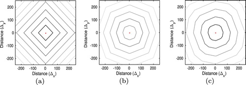
To demonstrate the improvement made by considering four stencils over only two stencils in capturing the anisotropic behaviour of the media, wave propagation through a single anisotropic crystal orientated by ${20}^{\circ }$ was modelled. Since we are considering a single homogeneous medium, evolution of the wave front should follow the shape of the inverse of the slowness curve rotated by ${20}^{\circ }$. Figure 2(a) demonstrates why the standard Higher Accuracy Fast Marching Method cannot be used. By only considering movement in horizontal and vertical directions, we obtain a wave front profile which moves with equal speed along these axes and does not correctly capture the altered symmetries of the slowness curve caused by the ${20}^{\circ }$ rotation of the crystal. By allowing the wave to travel along ${\mathcal{S}}_2$ the situation is improved and the result is shown in Figure 2(b). However, movement along the shorter arms of stencil ${\mathcal{S}}_1$ still dominates and the rotation of the crystal is not captured. By considering the additional stencils ${\mathcal{S}}_3$ and ${\mathcal{S}}_4$, the ${20}^{\circ }$ rotation of the axes of symmetry of the slowness curve is finally captured (see Figure 2(c)) and the wave propagation is slowest in the ${20}^{\circ }$ direction as expected (see [36]).

Figure 2. Contour plots of the travel time field (going from black to white as time increases) modelled by a fast marching based method when (a) stencil ${\mathcal{S}}_1$ is used, (b) both ${\mathcal{S}}_1$ and ${\mathcal{S}}_2$ are used and (c) when ${\mathcal{S}}_1,{\mathcal{S}}_2,{\mathcal{S}}_3$ and ${\mathcal{S}}_4$ are used (AMSFMM). The centre point marks the location of the source.

A more interesting example of the AMSFMM's ability to estimate the travel time field is shown in Figure 3. Here, a randomly generated Voronoi diagram was input into a finite element software package (Onscale [38]). Each Voronoi cell was assigned an orientation ${\varphi }_i$ and, using the elastic constants of austenitic steel, the anisotropic wave propagation through this random, locally anisotropic media was modelled. Thirty-two sources were placed on the top boundary of the domain and a pressure wave (with centre frequency 1.5 MHz) was sent into the material from each source in turn. The average time-variant, normal stress was then measured at 32 points along the bottom edge of the domain to simulate our receiving array [33]. These received waveforms were processed to extract the first times of arrival of the wave front (measured as the time at which the receiver is first subjected to a stress greater than ${10}^{-6}$Pa). These give the solid lines in Figure 3(b) for the case where the pressure wave was activated at transmitters s = 5, 14, 28, as indicated in Figure 3(a) along the top edge of the domain. The same map was then used within the AMSFMM algorithm (with a grid size of ${\mathrm{\Delta }}_x={\mathrm{\Delta }}_y=0.1$ mm which is comparable to the 0.13 mm element size employed within the FE simulation which is ultimately determined by the wavelength of the inspecting wave) to calculate the travel time to each point in the domain. The first times of arrival at each receiver were then interpolated from the grid points at depth 40 mm from the sources. These are plotted by the dashed lines in Figure 3(b) and good agreement between the two approaches is observed: not only are the general trends captured but more local features are also well matched, such as the longer travel times observed when transmitting on element 5 and receiving across the elements located between 7 and 12 mm along the x-axis. This is despite the fact that the times of arrival arising from the FE dataset are estimated at an arbitrarily chosen amplitude threshold (see Section 2.1) and so have an associated error tolerance. In terms of computational expense, for the parameters used in this scenario the AMSFMM implemented in Fortran provided an $\mathcal{O}({10}^2)$ speed up over the FE simulation (although note that this is only an indicative value as this improvement is largely dependent on the hardware and software used).

Figure 3. Plot (a) shows a randomly generated Voronoi tessellation with 100 seeds and a random assignment of orientations. Plot (b) compares the travel times from each of the sources s = 5, 14, 28 (marked by crosses on the top boundary) to all 32 receivers (placed at intervals of 2 mm along the bottom of the domain) through this geometry calculated using the finite element software (Onscale [38] – full line) and the AMSFMM (dashed line).

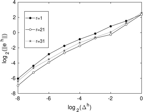
Having demonstrated the ability of the proposed numerical scheme to model the wave travel times through locally anisotropic structures, we present a brief study of its convergence. Using the same material model as presented in Figure 3, the travel times from a single transmitter to each receiver were computed using the AMSFMM on a series of grids with decreasing spacing. As the travel times estimated using the FE simulation are subject to some uncertainty, we compare our computed travel times, $T_0^h$, to a reference solution. $T_0^r$, generated using the AMSFMM computed on a grid with spacing ${\mathrm{\Delta }}_x={\mathrm{\Delta }}_y=1/512$ mm. We denote the absolute error between the estimated travel times and the reference solution by $\Vert e^h\Vert =\Vert T_0^h-T_0^r{\Vert }_2$, where h is the level of discretization (the side lengths are equal to ${\mathrm{\Delta }}^h=2^{1-h}$ mm for h = 1,…,9). Figure 4 plots the convergence of the travel times to the reference solution at three different receivers, r = 1, 21, 31, when the wave is initiated at source s = 12. It can be observed that $\Vert e^h\Vert$ converges linearly at an approximate rate of 1/2, which agrees with the convergence rates observed in [39] for the second-order FMM.

Figure 4. Convergence of the absolute travel time error to the reference solution at three receivers, r = 1, 21, 31 from source s = 12 (see Figure 3(a)). Here ${\mathrm{\Delta }}^h=2^{1-h}$ mm, $h=1,\dots ,9$, $\Vert e^h\Vert =\Vert T_0^h-T_0^r{\Vert }_2$, $T_0^r$ is the reference time of flight vector and $T_0^h$ is the corresponding time of flight vector for each grid size ${\mathrm{\Delta }}^h$.

2.4. A probabilistic framework

The reversible-jump Markov chain Monte Carlo (rj-MCMC) method produces a posterior distribution for transdimensional spaces (where the number of degrees of freedom of the model is not fixed). The posterior probability density function is given by Bayes' rule, $p(m|T_0)\propto p(T_0|m)p(m)$, where $p(m)$ is the a priori probability of the material model m and $p(T_0|m)$ is the likelihood that the observed time of flight data $T_0$ arises from that model. Since minimizing the misfit function is equivalent to maximizing the probability of a Gaussian likelihood function, we can write $p(T_0|m)\propto \exp (-\psi /2)$, where $\psi =\Vert (T_m-T_0)/{\sigma }_n{\Vert }^2$ is the least-squares misfit function between the observed and modelled data, and ${\sigma }_n^2$ is the variance of the noise present in the data which is discussed below. Following the approach taken in [23,40], we represent the prior probability density functions for each model parameter using uniform distributions over predefined ranges, informed by measured experimental parameters. Firstly, we allow the prior on the number of Voronoi cells used to parametrize the material's underlying structure, $p(M)$, to be defined by a discrete uniform distribution given by $p(M)=\{\begin{array}{ll}1/\mathrm{\Delta }M,& \mathrm{if}M\in \mathcal{M}\\ 0,& \mathrm{otherwise},\end{array}$ where $\mathcal{M}=[M_{min},M_{min}+1,\dots ,M_{max}-1,M_{max}]$, $\mathrm{\Delta }M=M_{max}-M_{min}+1$ and the bounds $M_{min},M_{max}\in \mathbb{Z}$ are chosen to reflect the wavelengths present in our system. The distribution that the crystal orientations ${\varphi }_i\in \mathrm{\Phi }$ can be drawn from, can be altered to reflect prior information on their distribution. However, to facilitate generalization to a wide class of applications, and to ensure transparency (as choosing a prior distribution that is close to the known material map would be advantageous to the reconstruction algorithm of course), we assume here that they are uniformly distributed $p({\varphi }_i)=\{\begin{array}{ll}1/\mathrm{\Delta }\varphi ,& \mathrm{if}{\varphi }_{min}\le {\varphi }_i\le {\varphi }_{max}\\ 0,& \mathrm{otherwise}.\end{array}$ By the same reasoning, we assume independence of the neighbouring crystal orientations and so we can write $p(\mathrm{\Phi }|M)=\prod _{i=1}^{M}p({\varphi }_i).$ Here, ${\varphi }_i$ is measured in degrees and $\mathrm{\Delta }\varphi ={\varphi }_{max}-{\varphi }_{min}+1$, where the bounds ${\varphi }_{min}=0$ and ${\varphi }_{max}=90$ are selected to reflect the symmetries of the slowness curve. Assuming that the seed positioning has a uniform probability distribution, and that our M seeds must have M distinct locations (that is the seeds cannot lie on top of each other), we have $p(S|M)={\left[\frac{|I_{\ast }|!}{M!(|I_{\ast }|-M)!}\right]}^{-1}$ where $|I_{\ast }|$ is the cardinality of our computational domain where the discretization is determined by the numerical precision with which the seed co-ordinates are assigned.

Finally, an important consideration to make when employing a transdimensional inversion scheme is the parametrization of the data uncertainty, which encompasses errors in data measurement and omission of complex physical phenomena from the forward model [41]. In this work, we treat the uncertainty as a single unknown which aggregates the aleatoric and epistemic uncertainties accumulated over each raypath. We allow the algorithm to infer the uncertainty level present in the system by drawing values from a uniform distribution over some predefined range, $p({\sigma }_n)=\{\begin{array}{ll}1/\mathrm{\Delta }{\sigma }_n,& \mathrm{if}{\sigma }_n^{min}\le {\sigma }_n\le {\sigma }_n^{max}\\ 0,& \mathrm{otherwise},\end{array}$ where $\mathrm{\Delta }{\sigma }_n={\sigma }_n^{max}-{\sigma }_n^{min}+1$ and we choose ${\sigma }_n^{min}=0.01\mu$s and ${\sigma }_n^{max}=1\mu$s (the average travel-times are around the order of 10μs). The level of uncertainty attributed to the dataset has a direct impact on the complexity of the solution: by restricting the range too much the algorithm will attempt to overfit the data, increasing the complexity of the model in order to minimize the data misfit, whilst permitting larger data uncertainties causes the model space to become large and difficult to search efficiently. The reader is referred to [23] for alternative and more in depth treatment of the noise parameter.

Given that we assume no prior knowledge of the covariance between the model parameters, we choose the partitioning of the spatial domain to be independent of the regional crystal orientation assignment and system noise level. The full a priori probability density function can then be written as a product of the probability density functions of the individual model parameters and so the a priori probability of a given model m is $p(m)=p(M)p(\mathrm{\Phi }|M)p(S|M)p({\sigma }_n)=\frac{M!(|I_{\ast }|-M)!}{\mathrm{\Delta }M(\mathrm{\Delta }\varphi {)}^M|I|!\mathrm{\Delta }{\sigma }_n},$ provided that the model parameters lie within their predefined ranges and is equal to 0 otherwise.

2.5. The reversible-Jump Markov chain Monte Carlo method

The reversible-jump Markov chain Monte Carlo method allows dimensional jumps in the model space which can later be reversed [22]. The process possesses the Markov property so that each perturbation of the model is dependent only on its current state and not on its history. To begin, a parametrization of the material microstructure m is constructed using a Voronoi tessellation. The initial number of cells is chosen arbitrarily and each cell is assigned a crystal orientation ${\varphi }_i$ drawn from a uniform distribution bounded by ${\varphi }_{min}$ and ${\varphi }_{max}$. For each pair of transmit-receive elements, the travel time field is modelled throughout the locally anisotropic geometry using the AMSFMM (see Section 2.3), and the time taken for the wave to propagate to each receiver is estimated. These travel times are compared with the first time of arrival information as extracted from the observed dataset and the posterior $p(m|T_0)$ for the initial model is calculated. The model is then perturbed to create a new model $m^{\prime }$. Large steps through the model space can alter the complexity of the solution towards which the algorithm converges [42], and so to avoid this potential problem the model parameters are perturbed independently to isolate their effects. Each perturbation is made subject to a proposal distribution, which represents the conditional probabilities of proposing a state $m^{\prime }$ given m. In this work, the model can be perturbed in one of five ways: a cell birth, death or move, a system noise change or a cell orientation change. Details of the proposals on the first four of these perturbations can be found in [5]. The perturbation of the orientation ${\varphi }_i$ in cell i is given by ${\varphi }_i^{\prime }={\varphi }_i+X{\sigma }_{\varphi }$ where $X\sim N(0,1)$ is a standard normal deviate with mean 0 and variance 1, and ${\sigma }_{\varphi }$ is the standard deviation of the proposal distribution for orientation. Once a perturbation has been made, the posterior $p(m^{\prime }|T_0)$ is calculated. The probability that a perturbation is accepted is subject to the Metropolis-Hastings criterion (5) $p(\text{accept})=min(1,\frac{p(m^{\prime }|T_0)}{p(m|T_0)}\times \frac{q(m|m^{\prime })}{q(m^{\prime }|m)}),$(5) where $q(m^{\prime }|m)$ is the proposal distribution; that is the probability of moving to model $m^{\prime }$ from m (the ratio of the reverse step $q(m|m^{\prime })$ to the forward step $q(m^{\prime }|m)$ is equal to one if the perturbation is not transdimensional) [42]. If $m^{\prime }$ is rejected, the model is discarded and the original model m is perturbed again. If accepted, the model $m^{\prime }$ replaces the model m and the process begins again.

Poor choices of standard deviations on the proposal distributions for the orientation, noise and geometry perturbations will result in a slow exploration of the model space. In our work, the proposal distributions are tuned until the acceptance rates lie somewhere between 23% and 44%, as declared optimal in [43]. A delayed rejection scheme (where secondary perturbations drawn from proposal distributions with smaller standard deviations are made on the rejection of the initial perturbation) has also been implemented to improve the efficiency of the model space search [44].

To generate a reliable estimate of the posterior, the model must be evaluated iteratively throughout the model space. After the initial sampling period (the burn in period), the Markov chain begins an importance sampling, favouring the higher likelihood regions of the model space. Ideally, the algorithm would be terminated when the Markov chain has converged: that is when the ensemble of models exhibits a density proportional to the posterior probability distribution. However, there exists no reliable method for the detection of convergence as it is effectively the measure of how well our estimate of the distribution represents the underlying, unknown stationary distribution of the Markov chain [45]. In this work, to best assess convergence, the misfit and data noise are monitored throughout the running of the algorithm to ensure that they are converging to values which align with our expectations based on our prior knowledge of the residuals between an observed dataset and a modelled dataset. Once we believe convergence has been achieved, the algorithm is terminated and the Markov chain of accepted models is sampled at an interval of κ, where κ is the relaxation time of the random walk (the number of steps required before we can expect to obtain a model that is considered independent of the last). In deterministic optimization schemes, the model with the smallest misfit (the global minimum) would typically be taken as the solution. Within the Bayesian framework, we consider the posterior distribution as a whole and instead of examining a single model, analyse various moments and characteristics of the distribution. To produce the mean image of the material map, we project the sampled partition models into the spatial domain and average. Given the large number of samples, when the Voronoi tessellations are stacked, the partitions overlap and the resulting regional orientation map is effectively a continuous function of the plane. It is also useful to study the median and maximum a posteriori (MAP) estimators at each point in the spatial domain, particularly if our posterior distribution is skewed or multi-modal. This framework also allows the study of the variance over the domain which can be exploited for uncertainty quantification studies and probability of detection work.

3. Results

3.1. Reconstruction of a synthetic material

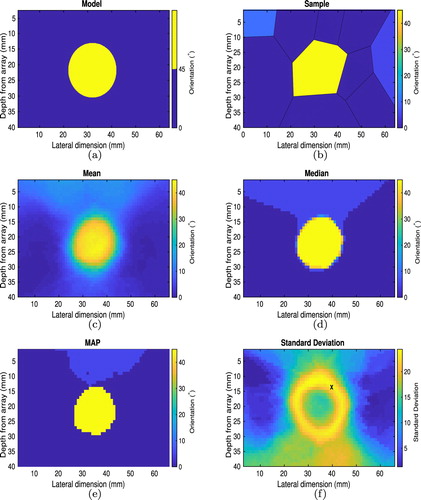
When many grains and orientations are present in a complex sample it can sometimes be difficult to visually assess the likeness of the reconstructed map with the known material geometry, particularly when we are primarily interested in the effective medium which will provide sufficient correction for defect imaging but may not accurately represent the structure well. Thus we will first examine the simplified case of a 20 mm diameter disc with assigned orientation of ${45}^{\circ }$ embedded in a host material with $0^{\circ }$ orientation (see Figure 5(a)), to allow visual comparison between the two. This example demonstrates that although we partition the domain using polygons, we can in fact reconstruct curved boundaries.

Figure 5. Material map reconstructions for a simplistic synthetic geometry. Plot (a) shows the true geometry input to the FE simulation to generate the observed time-of-flight matrx $T_0$. Plot (b) is an arbitrarily selected sample from the posterior distribution. Images (c), (d), (e) and (f) plot the mean, median, maximum a posteriori and standard deviation of the posterior distribution at each point in space, respectively. The observed data arose from a through-transmission phased array inspection of the geometry in (a) with a transmitting array spanning the top of the domain and a recording array spanning the base of the domain.

To construct synthetic data for this example, a phased array inspection (in the through-transmission format) was simulated in the finite element package Onscale [38] where the geometry was meshed with square elements with side lengths of approximately $260\mu$m. Absorbing boundary conditions were employed on the vertical edges of the domain to ensure energy was not reflected back into the domain at these edges (we assume the domain we are imaging forms only a subsection of a larger component). Free boundary conditions were assigned to the top and bottom edges of the domain on which the arrays were placed. A 1.5MHz sinusoidal pulse (giving rise to a wavelength of approximately $\lambda =3.8$ mm) was used to excite the system which consisted of two 32 element phased arrays placed directly opposite each other on either side of the rectangular component. The arrays had a pitch (element spacing) of 2 mm and the depth of the component was 40 mm. It is important to note that the Onscale software models many of the physical phenomena present in the ultrasonic phased array inspection, for example mode conversion and diffraction, and it has previously been validated against experimental data [33]. We treat these aspects of the data as system noise. Coupled with the subjectivity involved in selecting the first time of arrival from the simulated time-domain data, the levels of uncertainty present in the simulated data imitate those present in experimentally collected data and so the addition of synthetic noise is not required here. The resulting time-of-flight matrix $T_0$ then serves as the observed data for the rj-MCMC.

An arbitrary set of seeds S and orientations Φ drawn from uniform distributions were used to construct the initial Voronoi diagram. The rj-MCMC algorithm was run for 50,000 samples and assumed to be stationary after 10,000 samples. These initial 10,000 samples were discarded (the so-caled burn in period) and the remaining models were sampled at an interval of $\kappa =100$; it is these sampled models from which our statistics are drawn. Figure 5(b) depicts an arbitrary sample drawn from the posterior distribution, and it can be observed that the algorithm is sampling from the correct area of the model space (that is it resembles the known geometry). Taking the mean of the posterior distribution for this case, we obtain the map shown in Figure 5(c). We can also study the median of the posterior distribution on orientation at each point in the domain (Figure 5(d)) and the maximum-a-posteriori (MAP - Figure 5(e)). Interestingly, if we study the posterior distribution of a point lying on the high uncertainty loop observed in the standard deviation map (as marked by the cross in Figure 5(f)), a bimodal distribution is observed (data not shown for brevity) which suggests that the problem is poorly constrained on the boundary of the anomaly; the pixels here may lie in either of the two regions as the data are not sufficient to discriminate. This can be viewed as a nonlinear measure of spatial resolution [24] and also explains the midrange values present on the boundary of the anomaly (circa 20° in the mean image (Figure 5(c))).

3.2. Simulated inspection of an austenitic weld

Moving now to a more realistic NDT scenario, FE simulations of the ultrasonic phased array inspection of an austenitic weld were run in the software package Onscale [38] using electron backscatter diffraction (EBSD) measurements taken from an austenitic weld (the macrographic details of this weld structure can be found in [32]). These measurements were processed to provide a coarse map of the weld microstructure, resulting in a simplified representation of the weld microstructure [32,46]. This map was input into the FE model and meshed with elements with dimension equal to $\lambda /15$ (where λ is the smallest wavelength in the system). A 1.5 MHz centre frequency was used and the minimum shear wave speed was assumed to be 3000 m s${}^{-1}$, giving way to a correlation length (between the wavelength and grain structure) of around $\lambda /8$ [47] and an element size of approximately $133\mu$m (this is below the Rayleigh scatterer limit and sufficient to model accurate wave propagation [32]). As before, a through-transmission set up was chosen to allow easy extraction of the first time of arrivals for each transmit-receive pair. This involved two 50 element arrays, with 2 mm pitch, placed directly opposite each other on either side of the weld. The resulting FMC dataset was processed to yield the time of flight matrix and this was taken as the input for the rj-MCMC algorithm.

The rj-MCMC algorithm was run for 1,000,000 samples, and stationarity was assumed after 250,000 samples which were discarded as the burn-in period. The remainder were sampled at a rate of $\kappa =100$ to ensure that the ensemble was constructed from independent samples. It is important to note here that included in the reconstruction domain are areas of the isotropic stainless steel parent material with wave speed 5790m  s${}^{-1}$ (the weld can be imagined as a central V-shaped section of the rectangular domain sandwiched between our two linear arrays). To produce optimal results, an approximation of the V-shaped weld domain was assumed to be known a priori (in practice, the outline of the weld region can often be seen on the surface of the sample and so it is not unrealistic to exploit this information). The rj-MCMC was adapted so that if a Voronoi seed lay outside of the defined weld region (marked by black solid lines in Figure 6(c)), its cell was treated as isotropic (that is independent of incident wave direction) with wave speed 5790m  s${}^{-1}$. Due to the dynamic nature of the material partitioning, these weld outlines could be perturbed by the inversion process to adapt to the time of flight data, allowing flexibility in how the algorithm perceives the properties of areas such as the heat affected zone (HAZ) at the parent-weld interface. Failing to consider the parent material's isotropic nature negatively effected convergence of the method as the model struggled to explain the behaviour of the wave in this region.

Figure 6. Effective orientation maps of the weld geometry reconstructed by the rj-MCMC. Plot (a) depicts the mean of the posterior distribution at each point of the spatial domain. Plots (b)–(d) depict the median, MAP estimator and standard deviation respectively. The observed data arose from the through-transmission phased array inspection of the weld geometry with a transmitting array spanning the top of the domain and a recording array spanning the base of the domain.

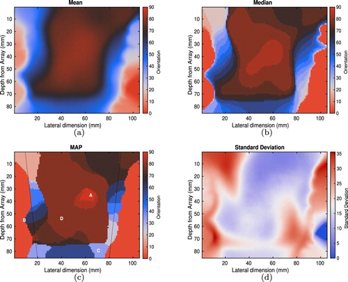
Figures 6(a–d) depict maps of the mean, median, maximum a posteriori (MAP) and standard deviation of the posterior distributions on effective orientation reconstructed by the rj-MCMC at each point within the inspection domain. Note that the isotropic regions which model the parent material are assigned $0^{\circ }$ orientation here for the purposes of visualization, but given that the slowness curve assigned to these regions is circular with a constant velocity value of 5790m  s${}^{-1}$, these orientations could be arbitrarily selected. These isotropic regions can be seen very clearly in both the median and MAP reconstructions (plots (b) and (c), respectively) and it is clear that the dynamic partitioning has caused perturbations to the outline of the weld region as these differ between the two plots. This effect is also manifested in the high standard deviation values in plot (d). 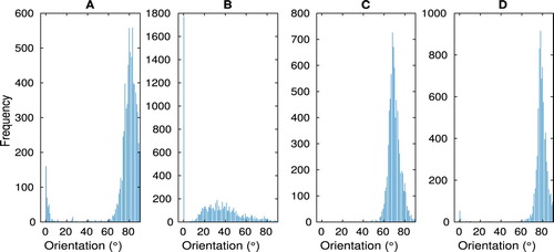Due to the fact that crystals with rotation $0^{\circ }$ behave like crystals with orientation ${90}^{\circ }$ (this is reflected in the cyclic colour scheme), the posterior distribution on orientation at some points is bi-modal and this results in a poorly resolved estimation of the material map by the mean since it averages across multiple modes. Consequently, we claim that the MAP estimator better represents the underlying posterior distributions as it better preserves the discontinuities between regions, and so we will use this as the basis of the TFM+ imaging algorithm in Section 3.2.2. Histograms depicting the posterior distributions of the orientation at four points in the spatial domain (as marked A–D in Figure 6(c)) have been plotted in Figure 7 and this bimodal distribution can be observed in the posterior distributions at point A (and to a much lesser extent at point D). Point B of Figure 6(c) lies on the boundary of the weld region and the algorithm fails to fully resolve whether this lies in the weld region or in the parent region and this manifests in a large number of samples which assign this particular pixel $0^{\circ }$ orientation (as is our practice for points outside the weld domain). This is also reflected in the posterior distribution on material classification at this point (that is whether it is anisotropic or isotropic – these two phase plots are omitted for brevity) which also exhibits a bimodal distribution and hence a high level of uncertainty.

Figure 7. The estimated posterior distributions on orientation at four distinct points in the map (as depicted in Figure 6(c)) generated from the inversion of the simulated ultrasonic array data arising from the inspection of the weld geometry.

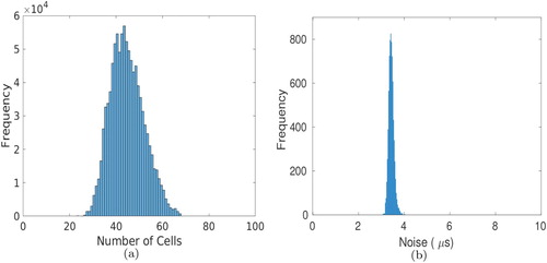
Recall that in this transdimensional approach, the number of cells M which partition the spatial domain, is itself a parameter to be inverted, as is the level of aggregated noise ${\sigma }_n$. The posterior probability density functions $p(M|d_{obs})$ and $p({\sigma }_n|d_{obs})$ are shown in Figure 8(a,b), respectively. Although the structure of the true model is complex, the natural parsimony of the Bayesian approach [42] results in a posterior on the number of cells with a surprisingly low mean of 43 cells. This is likely to be due to the fact that the time of flight data is insufficient to fully constrain the problem and capture the fluctuations on orientation at the microstructural level, resulting in resolution of the anisotropic trends on a macro-scale. The low variance PDF on noise lying within the expected range as shown in Figure 8(b) suggests that for this case it is enough to study the single aggregated noise parameter ${\sigma }_n$ and the more complex noise models as explored in [24] are not required here (potentially due to the enhanced and even coverage afforded by NDE inspections compared to that used within a seismology setting).

Figure 8. The estimated posterior distributions on (a) the number of cells M used to partition the spatial domain and (b) the noise parameter ${\sigma }_n$, from the inversion of the simulated ultrasonic array data arising from the inspection of the weld geometry.

3.2.1. The total focussing method

To account for our reconstructed anisotropic grain map, we employ the AMSFMM to create a new imaging technique; as it is a natural extension of the TFM we denote it TFM+. Treating each transmitting element in turn as a source, a set of N travel-time fields ${\tau }^s(x,y)$, $s=1,\dots N$, through the reconstructed material map are generated using the AMSFMM, providing us with the travel-times to each pixel in the imaging domain from each source. Since source-receiver reciprocity holds, these travel-time fields also represent the time taken for the wave to travel from each pixel back to each receiver. To create an image of our inspection domain, the reflectivity at each pixel is therefore given by (6) $w_{i,j}=\left|\sum _{s=1}^N\sum _{r=1}^N{A}_{s,r}({\tau }^s(x_i,y_j)+{\tau }^r(x_i,y_j))\right|,$(6) where ${\tau }^s(x_i,y_j)$ is the time taken for the wave to travel from source s to the pixel $(x_i,y_j)$ and, similarly, ${\tau }^r(x_i,y_j)$ is the time taken for the wave to travel from the pixel $(x_i,y_j)$ to the receiver r.

3.2.2. Flaw reconstruction results

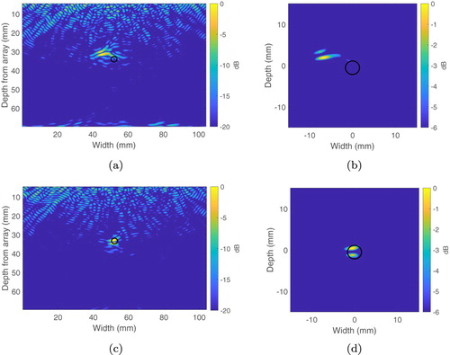
Here, the success of the reconstructed weld map is measured via its use in conjunction with the TFM+ algorithm in application to a one-sided (pulse-echo) inspection dataset in which a 3 mm diameter void is located centrally, 33.8 mm below the centre of the array. The flaw reconstruction displayed in Figure 9(a) arises from application of the standard TFM to the dataset where a constant wave speed of 5790m  s${}^{-1}$ (that of the parent material) is assumed throughout the domain and the plot is normalized with respect to its highest amplitude and plotted over a dynamic range of 20 dB. A $30\times 30$ mm region centred on the known location of the flaw is shown in Figure 9(b) and is plotted over a dynamic range of −6 dB (the measurement threshold). Although the presence of a scatterer is clearly detected, the energy is dispersed and does not lie within the known domain of the flaw as marked by the black disc. The reconstruction of a locally anisotropic grain map of the weld via the rj-MCMC algorithm (we use the MAP estimator – see Figure 6(c)) was used to provide correction to the TFM imaging algorithm via Equation (6(6) $w_{i,j}=\left|\sum _{s=1}^N\sum _{r=1}^N{A}_{s,r}({\tau }^s(x_i,y_j)+{\tau }^r(x_i,y_j))\right|,$(6) ) (TFM+), and the results are shown in Figure 9(c). Image (d) shows the area local to the flaw (again plotted at -6dB) and we observe a significant improvement in the concentration of energy near the known location of the scatterer compared to that shown in Figure 9(b). If we take the highest amplitude point in image (b) as an indication of the flaw location, this is 6.8 mm away from the known centre of the flaw, compared to an error in placement of only 0.6 mm in image (d). Taking the flaw diameter to be the length of the region which lies above the −6dB threshold (along the largest dimension), then the standard TFM gives rise to a measurement of 6.2 mm whilst the TFM+ reconstructs a scatterer with diameter 3.7 mm. It is worth noting that both the median and mean maps shown in Figure 6 gave rise to a similar level of improvement when applied in conjunction with the TFM to this data set. Although the mean map appears to lack sufficient detail, it captures the overall global trend and provides reasonable correction to the waves skewed by the anisotropic behaviour of the material.

Figure 9. Image (a) arises from application of the standard TFM algorithm with a constant wave speed $c_l=5790$ m s${}^{-1}$ (that of the parent material) assumed throughout the domain. Image (b) is a close up of a $30{\text{mm}}^2$ region centred on the known location of the flaw, plotted at the -6dB measurement threshold. Image (c) depicts the results when the material orientation map reconstructed by the rj-MCMC in Figure 6(c) is used in conjunction with the TFM+ imaging algorithm and image (d) is a close up of the $30{\text{mm}}^2$ region centred on the known location of the flaw. The black discs depict the actual size, shape and location of the defect.

4. Conclusions and discussion

A stochastic, transdimensional optimization approach for reconstructing maps of spatially varying crystal orientations in polycrystalline media from ultrasonic array measurements has been put forward in this paper. An efficient forward model for wave propagation within complex, locally anisotropic media was presented and it was shown that this could provide sufficiently good estimates of the travel times of longitudinal waves in this class of materials. It was then demonstrated that use of this model within the rj-MCMC inversion framework could be successfully used to generate an approximation of the material map which in turn could be exploited by a delay and sum style imaging algorithm (here, the TFM). In doing so, improvements were achieved in flaw detection, flaw placement and flaw characterization. In the case of a 3 mm diameter void embedded centrally below the array at a depth of 33.8 mm, a 6.2 mm improvement in flaw placement and a 2.5 mm improvement in flaw measurement was achieved.

It must be noted that in its current form, this methodology does not allow us to draw fair quantitative comparisons between the known material map and the reconstructed map. There exist several reasons behind this. Firstly, the rj-MCMC reconstructs an effective medium, that is a representation of the material which will correct the travel times of the propagating wave but may not accurately represent the microstructure of the weld itself (in fact unphysical artefacts may enter the reconstruction, for example the presence of crystals with 45 degree orientation at the bottom of the weld as in 6). The difference between this effective medium and the underlying microstructure used in the FE simulation can be attributed in part to model simplifications (for example reducing the dimension of the model space by only considering grain orientations which lie between $0^{\circ }$ and ${90}^{\circ }$), and in part to the approximation of the weld as a transversely isotropic solid with the associated simplification of considering crystal rotations in the xz plane only. This heterogeneous effective medium proves to be sufficient for the purposes of demonstrating the methodology in this paper and the resulting flaw image improvement. However, if we want to reconstruct an accurate representation of the crystalline structure itself (perhaps for use at the manufacturing stage to monitor the texture of the weld), a more sophisticated forward model within the inversion framework is required; the Eikonal equation, with its basis in ray theory, only provides a good approximation of wave front propagation in the high-frequency regime, meaning it does not well model velocity variations which occur on a scale smaller than the wavelength [48]. This can be seen in Figure 6, where the reconstructions show variations in crystal orientation on a very coarse scale (much greater than the millimetre order of the wavelength). To refine the resolution of the reconstructed maps, more wave physics (diffraction for example [49]) must be included. Additionally, the array pitch must be reduced to increase the coverage of the domain. Of course, full aperture inspection (where transducers are placed over the entire boundary, encircling the component) would also further constrain the problem and enhance the resolution, however for NDT applications this is not often possible in practice due to restrictions on surface access. In fact, even the through transmission acquisition geometry presented in this paper will rarely be applicable in the field due to limited surface access and the weld cap geometry. Consideration of a pitch catch inspection where both arrays are mounted on wedges on the top surface of the weld is currently underway but a reduced coverage of the weld by the ray paths means that this is a non-trivial extension. Further to these practical constraints, addition of more sources and receivers is computationally demanding.

Another consequence of the coarse resolution of the reconstructions obtained in this work is that we are forced to ignore the sub-wavelength defect properties within the rj-MCMC framework itself. Similar to the approach taken for including the isotropic parent material, it would be possible to allow the Voronoi cells to adopt the material properties of air say, and thus allow the algorithm to invert the location and nature of any embedded flaws. However, since we are interested primarily in sub-wavelength defects, the time of flight data on which the method is applied lacks sufficient sensitivity to their presence: currently, the delay in time of flight caused by a small flaw lies within the noise level of the inversion method. Thus we require the subsequent application of the TFM+ to exploit the full waveform data and successfully resolve the sub-wavelength defects

Data statement

All data presented in this publication can be reproduced using the OnScale finite element model and associated parameters made available at the University of Strathclyde KnowledgeBase at https://doi.org/10.15129/a090b49a-7977-4802-80ae-0a7ddd1053ef

Acknowledgments

The authors would also like to thank the Edinburgh Interferometry Project (EIP) sponsors (Schlumberger Cambridge Research, Equinor and Total) for supporting this research.

Disclosure statement

No potential conflict of interest was reported by the authors.

Additional information

Funding

This work was funded by the Engineering and Physical Sciences Research Council (EPSRC) (grant numbers EP/S001174/1 and EP/P005268/1) with support from EDF, the National Nuclear Laboratory, the National Physical Laboratory, Onscale and Rolls Royce.

References

- Holmes C, Drinkwater BW, Wilcox PD. Post processing of the full matrix of ultrasonic transmit receive array data for non destructive evaluation. NDT E Int. 2005;38(8):701–711.
- Camacho J, Parrilla M, Fritsch C. Phase coherence imaging. IEEE Trans Ultrason Ferroelectr Freq Control. 2009;56(5):958–974.
- Connolly GD, Lowe MJS, Temple JAG, Rokhlin SI. The application of fermat's principle for imaging anisotropic and inhomogeneous media with application to austenitic steel weld inspection. Proc R Soc A Math Phys Engin Sci. 2009;465:3401–3423.
- Zhang J, Hunter A, Drinkwater BW, et al. Monte carlo inversion of ultrasonic array data to map anisotropic weld properties. IEEE Trans Ultrason Ferroelectr Freq Control. 2012;59(11):2487–2497.
- Tant KMM, Galetti E, Curtis A, et al. A transdimensional bayesian approach to ultrasonic travel-time tomography for non-destructive testing. Inverse Probl. 2018;34(9):095002.
- Nageswaran C, Carpentier C, Tse YY. Microstructural quantification, modelling and array ultrasonics to improve the inspection of austenitic welds. Insight-Non-Destruct Test Condition Monitor. 2009;51(12):660–666.
- Ogilvy JA. Computerized ultrasonic ray tracing in austenitic steel. NDT Int. 1985;18(2):67–77.
- Gueudré C, Le Marrec L, Moysan J, et al. Direct model optimisation for data inversion. application to ultrasonic characterisation of heterogeneous welds. NDT E Int. 2009;42(1):47–55.
- Chassignole B, Villard D, Dubuget M, et al. Characterization of austenitic stainless steel welds for ultrasonic NDT. AIP Conf. Proc. 2000;509(1):1325–1332.
- Sharples SD, Clark M, Somekh MG. Spatially resolved acoustic spectroscopy for fast noncontact imaging of material microstructure. Opt Express. 2006;14(22):10435–10440.
- Abrahams ID, Wickham GR. The propagation of elastic waves in a certain class of inhomogeneous anisotropic materials. I. the refraction of a horizontally polarized shear wave source. Proc R Soc A Math Phys Engin Sci. 1992;436:449–478.
- Connolly GD, Lowe MJS, Temple JAG, et al. Correction of ultrasonic array images to improve reflector sizing and location in inhomogeneous materials using a ray-tracing model. J Acoustic Soc Am. 2010;127(5):2802–2812.
- Spies M. Analytical methods for modeling of ultrasonic nondestructive testing of anisotropic media. Ultrasonics. 2004;42(1):213–219.
- Harvey G, Tweedie A, Carpentier C, et al. Finite element analysis of ultrasonic phased array inspections on anisotropic welds. AIP Conf. Proc. 2010;1335:827–834.
- Lane C. The development of a 2D ultrasonic array inspection for single crystal turbine blades. Cham, Switzerland: Springer Science & Business Media; 2013.
- Fan Z, Mark AF, Lowe MJS, et al. Nonintrusive estimation of anisotropic stiffness maps of heterogeneous steel welds for the improvement of ultrasonic array inspection. IEEE Trans Ultrason Ferroelectr Freq Control. 2015;62(8):1530–1543.
- Chassignole B, El Guerjouma R, Ploix MA, et al. Ultrasonic and structural characterization of anisotropic austenitic stainless steel welds: towards a higher reliability in ultrasonic non-destructive testing. NDT E Int. 2010;43(4):273–282.
- Lhuillier PE, Chassignole B, Oudaa M, et al. Investigation of the ultrasonic attenuation in anisotropic weld materials with finite element modeling and grain-scale material description. Ultrasonics. 2017;78:40–50.
- Moysan J, Apfel A, Corneloup G, et al. Modelling the grain orientation of austenitic stainless steel multipass welds to improve ultrasonic assessment of structural integrity. Int J Pressure Vessels Piping. 2003;80(2):77–85.
- Mark AF, Fan Z, Azough F, et al. Investigation of the elastic/crystallographic anisotropy of welds for improved ultrasonic inspections. Mater Charact. 2014;98:47–53.
- Ogilvy JA. Ultrasonic beam profiles and beam propagation in an austenitic weld using a theoretical ray tracing model. Ultrasonics. 1986;24(6):337–347.
- Green PJ. Reversible jump markov chain monte carlo computation and bayesian model determination. Biometrika. 1995;82(4):711–732.
- Galetti E, Curtis A, Baptie B, et al. Transdimensional Love-wave tomography of the British Isles and shear-velocity structure of the East Irish Sea Basin from ambient-noise interferometry. Geophys J Int. 2016;208(1):36–58.
- Galetti E, Curtis A, Meles GA, et al. Uncertainty loops in travel-time tomography from nonlinear wave physics. Phys Rev Lett. 2015;114(14):148501.
- Gueudré C, Mailhé J, Ploix M-A, et al. Influence of the uncertainty of elastic constants on the modelling of ultrasound propagation through multi-pass austenitic welds. impact on non-destructive testing. Int J Pressure Vessels Piping. 2019;171:125–136.
- Popovici AM, Sethian JA. 3-D imaging using higher order fast marching travel times. Geophysics. 2002;67(2):604–609.
- Drinkwater BW, Wilcox PD. Ultrasonic arrays for non-destructive evaluation: a review. NDT E Int. 2006;39(7):525–541.
- Virieux J, Operto S. An overview of full-waveform inversion in exploration geophysics. Geophysics. 2009;74(6):WCC1–WCC26.
- Nguyen LT, Modrak RT. Ultrasonic wavefield inversion and migration in complex heterogeneous structures: 2d numerical imaging and nondestructive testing experiments. Ultrasonics. 2018;82:357–370.
- Van Pamel A, Brett CR, Huthwaite P, et al. Finite element modelling of elastic wave scattering within a polycrystalline material in two and three dimensions. J Acoustic Soc Am. 2015;138:2326–2336.
- Okabe A, Boots B, Sugihara K, et al. Spatial tessellations concepts and applications of Voronoi diagrams. Chichester, England: Wiley; 2009.
- Harvey G, Tweedie A, Carpentier C, et al. Finite element analysis of ultrasonic phased array inspections on anisotropic welds. AIP Conf. Proc., 2010 18–23 Jul; San Diego (CA); Vol. 1335. p. 827–834.
- Dobson J, Tweedie A, Harvey G, et al. Finite element analysis simulations for ultrasonic array nde inspections. In AIP Conf. Proc. AIP Publishing; 2016; Vol. 1706, p. 040005.
- Sethian JA. Fast marching methods. SIAM Rev. 1999;41(2):199–235.
- Rawlinson N, Sambridge M. Wave front evolution in strongly heterogeneous layered media using the fast marching method. Geophys J Int. 2004;156(3):631–647.
- Connolly GD. Modelling of the propagation of ultrasound through austenitic steel welds [PhD thesis]. London: Imperial College London (University of London); 2009.
- Hassouna MS, Farag AA. Multistencils fast marching methods: A highly accurate solution to the eikonal equation on cartesian domains. IEEE Trans Pattern Anal Mach Intell. 2007;29(9):1563–1574.
- OnScale. 770 Marshall Street, Redwood City, CA 94063.
- Rawlinson N, Sambridge M. Multiple reflection and transmission phases in complex layered media using a multistage fast marching method. Geophysics. 2004;69(5):1338–1350.
- Bodin T, Sambridge M, Gallagher K. A self-parametrizing partition model approach to tomographic inverse problems. Inverse Probl. 2009;25(5):055009.
- Bodin T, Sambridge M, Rawlinson N, et al. Transdimensional tomography with unknown data noise. Geophys J Int. 2012;189(3):1536–1556.
- Galetti E, Curtis A. Transdimensional electrical resistivity tomography. J Geophysic Res Solid Earth. 2017.
- Gelman A, Roberts GO, Gilks WR. Efficient Metropolis jumping rules. Bayesian Stat. 1996;5:599–608.
- Green PJ, Mira A. Delayed rejection in reversible jump metropolis–hastings. Biometrika. 2001;88(4):1035–1053.
- Cowles MK, Carlin BP. Markov chain Monte Carlo convergence diagnostics: a comparative review. J Am Stat Assoc. 1996;91(434):883–904.
- Carpentier C, Nageswaran C, Tse YY. Evaluation of a new approach for the inspection of austenitic dissimilar welds using ultrasonic phased array techniques. In Proc 10th ECNDT conference, (ECNDT, Moscow, 2010). 2010; p. 442–444.
- Cunningham LJ, Mulholland AJ, Tant KMM, et al. The detection of flaws in austenitic welds using the decomposition of the time-reversal operator. Proc R Soc A Math Phys Engin Sci. 2016;472(2188):20150500.
- Nolet G. A breviary of seismic tomography. Cambridge: Cambridge University Press; 2008.
- Huthwaite P, Simonetti F. High-resolution imaging without iteration: a fast and robust method for breast ultrasound tomography. J Acoustic Soc Am. 2011;130(3):1721–1734.