Solving generalized inverse eigenvalue problems via L-BFGS-B method

ABSTRACT

The parameterized generalized inverse eigenvalue problems containing multiplicative and additive inverse eigenvalue problems appear in vibrating systems design, structural design, and inverse Sturm–Liouville problems. In this article, by using the Cholesky factorization and the Jacobi method, we propose two efficient algorithms based on Newton's method and the L-BFGS-B method for solving these problems. To demonstrate the effectiveness of the algorithms, we present three numerical examples.

Keywords:

• Inverse eigenvalue problem
• parameterized generalized inverse eigenvalue problems
• Cholesky factorization
• L-BFGS-B method
• Jacobi rotation
• Newton's method

AMS MSC 2010:

• 65F18
• 49M15

1. Introduction

In the eigenvalue problems, the information contains the elements of a matrix or a matrix pencil and the unknowns of these problems include all or some of the eigenvalues. Describing and solving these problems by using some effective methods are found in [1,2]. But in the corresponding inverse problems, the data contains the complete information, or part of the eigenvalues or eigenvectors. In fact, the inverse problems include finding a matrix or matrix pencils according to the given information under spectral and structural constraints [3–6]. The current literature on the inverse eigenvalue problems shows that the creation of the inverse eigenvalue problems are inevitable in practical applications. Inverse eigenvalue problems, according to the application may be seen in different forms. In [3], a set of inverse eigenvalue problems was recognized and categorized according to its specifications. A lot of inverse eigenvalue problems are generalized inverse eigenvalue problems. Since many physical problems can be modelled as generalized inverse eigenvalue problems, many different examples of these problems have appeared. For example, the generalized inverse eigenvalue problem over the Hermitian–Hamiltonian matrices with a submatrix constraint was studied in [7]. In [8], Liu et al. considered the generalized inverse eigenvalue problem for centrohermitian matrices. In [9], the generalized inverse eigenvalue problem for generalized snow-like matrices was investigated. A generalized inverse eigenvalue problem in structural dynamic model updating was studied in [10]. In [11], a generalized inverse eigenvalue problem by the Jacobi matrix was considered. In these problems, a set of eigenvalues and a matrix pencil function that contained unknown parameters are given and the goal is finding unknown parameters under some conditions. Due to their many applications, these problems have always been a concern for researchers [12,13].

To simplify the discussion, we introduce the following notation. The symbols ${\mathcal{H}}_n$ and ${\mathcal{U}}_n$ stand for the sets of all $n\times n$ upper triangular matrices and $n\times n$ lower triangular matrices, respectively. We use A>0 and $A\ge 0$, when the matrix A is a positive definite matrix and positive semi-definite matrix, respectively. The symbol $\Vert .\Vert$ represents the Euclidean norm for vectors and induced norms for matrices. In addition, we denote a matrix pencil pair briefly with the notation $(A,B)$.

The parameterized generalized inverse eigenvalue problem (PGIEP) can be described as follows:

Definition 1.1

Let $A(c)=A(c_1,c_2,\dots ,c_n)$ and $B(c)=B(c_1,c_2,\dots ,c_n)$ be two given $n\times n$ matrices whose entries are analytic functions of parameters $(c_1,c_2,\dots ,c_n)$. Given n real numbers ${\lambda }_1,{\lambda }_2,\dots ,{\lambda }_n$, find $c\in {\mathbb{R}}^n$ such that the generalized eigenvalue problem $A(c)x=\lambda B(c)x$ has the prescribed eigenvalues ${\lambda }_1,{\lambda }_2,\dots ,{\lambda }_n$.

In many practical applications, such as structural design [14–16], the pencil matrix pair $(A(c),B(c))$ is affine that causes the creation of the special cases of the PGIEP. In this paper, we consider the special case of this problem in the form below:

Problem 1.1

As special type of the PGIEP, in this problem, we set (1) $A(c)=A_0+\sum _{i=1}^n{c}_i{A}_i,B(c)=B_0+\sum _{i=1}^n{c}_i{B}_i,$(1) where $A_i,$ $i=0,1,2,\dots ,n,$ are $n\times n$ symmetric matrices, $B_0>0,$ $B_i\ge 0$ for $i=1,2,\dots ,n,$ and the given eigenvalues ${\lambda }_1,{\lambda }_2,\dots ,{\lambda }_n$ are ordered as ${\lambda }_1<{\lambda }_2<\cdots <{\lambda }_n$.

The algebraic inverse eigenvalue problem [17] and the additive inverse eigenvalue problems [18] are two special types of Problem 1.1.

Problem 1.1 is considered as one of the most frequent inverse eigenvalue problems that appears in various areas of mathematical and numerical analysis and engineering applications [19–22]. Actually, Problem 1.1 arises in a variety of practical applications of structural engineering, mechanics, and physics. Some of these applications are as follows [14,23,24]:

• Studying a vibrating string and [25,26];

• Nuclear spectroscopy;

• The educational testing problem;

• The graph partitioning problem;

• Sturm–Liouville problems and preconditioning;

• Factor analysis [27] and the design of control systems [18].

We will now describe several examples arising in various areas of applications.

Application 1.1

[28]

Consider inverse Sturm–Liouville problems as follows: (2) $\begin{array}{rl}-\ddot{u}(x)+p(x)u(x)& =\lambda u(x)\end{array}$(2) (3) $\begin{array}{rl}u(0)& =u(\pi )=0,\end{array}$(3) where the purpose is to determine the density function $p(x)>0$ viewing the eigenvalues $\{{\lambda }_i^{\ast }{\}}_1^{\mathrm{\infty }}$. Using finite differences to solve these problems leads to the inverse eigenvalue problem as follows$:$ $Au+Du={\lambda }_i^{\ast }u,i=1,2,\dots ,n,$ in which the goal is to find the matrix $D=\mathrm{diag}(d_1,d_2,\dots .d_n)=\mathrm{diag}(p(h),p(2h),\dots ,p(nh))>0$. This is a classical example of the parameterized generalized inverse eigenvalue problems.

Application 1.2

It is showed in [29] that a vibrational mass-spring set can be modelled as a system of ordinary differential equations as fallow: $\dot{x}=Ax,$ where the multiplied matrix of this system is a symmetric matrix of physical parameters like $A=\left[\begin{array}{ccccc}{k}_1+k_2& -k_2& & & \\ -k_2& k_2+k_3& -k_3& & \\ & -k_3& k_3+k_4& -k_4& \\ & & \ddots & \ddots & \ddots \\ & & & -k_n& k_n\end{array}\right],$ and $x\in R^n$. It is possible to write A as the following linear combination of physical parameters $A=A(c)=A_0+\sum _{i=1}^n{c}_i{A}_i,$ where $\begin{array}{rl}& c_i=k_i,B_0=I,B_i=0,i=1,2,\dots ,n,\\ & A_0=0,A_1=e_1{e}_1^{\mathrm{T}},A_i=(e_{i-1}-e_i)(e_{i-1}-e_i{)}^{\mathrm{T}},i=2,3,\dots ,n,\end{array}$ when it is assumed that we have the natural frequency of the system as eigenvalues of A, finding the matrix is changed to determining the multipliers $c_i>0,i=1,2,\dots ,n$.

Also Problem 1.1 plays an important role in structure design and applied mechanics [19].

Application 1.3

In many practical applications of structures with l elements and n displacement degrees of freedom, such as, truss structure design, by assuming that $c=(c_1,c_2,\dots ,c_l)$ is a set of design parameters, the global stiffness matrix $A(c)$ and global mass matrix $B(c)$ are defined as: $\begin{array}{rl}A(c)& =c_1{K}_1+c_2{K}_2+\cdots +c_l{K}_l,\\ B(c)& =M_0+c_1{M}_1+c_2{M}_2+\cdots +c_l{M}_l,\end{array}$ where $K_i$ and $M_i$ are the stiffness and mass matrices of the ith element of the structure. In these problems, the goal is to determine $c_i>0,i=1,2,\dots ,l$ such that it is the set $\{{\lambda }_1^{\ast },{\lambda }_2^{\ast },\dots ,{\lambda }_l^{\ast }\}$of the eigenvalues of the generalized eigenvalue problem $A(c)x=\lambda B(c)x$.

On the other hand, various applications of the PGIEP have made it a favourite topic for analysis. Many recent studies have focused on the numerical methods and existence theory for different categories of these problems [3,30,31]. Sufficient and necessary conditions for the solvability of the specific types of the PGIEP were presented in [18,31–36]. In addition, in [37], Dai et al. presented sufficient conditions for guaranteeing the existence of a solution for the parameterized generalized inverse eigenvalue problem. More results in this area can be found in [38,39].

Further more, a review of recent literature on inverse eigenvalue problems shows that there are plenty of results for finding the answer to the PGIEP. In general, different approaches have been used to solve these problems according to their types. These methods can be categorized into three main categories of direct methods, iterative methods and continuous methods [3]. However the similarity of these methods is the confrontation with a nonlinear system of equations or an optimization problem. Since the nonlinear system of equations is simpler in repetitive and continuous methods, these methods have been extensively considered in recent years [3]. Also iterative methods were developed for solving the specific types of the PGIEP [40–42]. Formulations of some of these methods were defined by solving the following nonlinear systems (4) $\begin{array}{rl}F(c)& =\left[\begin{array}{c}{\lambda }_1(c)-{\lambda }_1\\ {\lambda }_2(c)-{\lambda }_2\\ ⋮\\ {\lambda }_n(c)-{\lambda }_n\end{array}\right]=0,\end{array}$(4) (5) $\begin{array}{rl}F(c)& =\left[\begin{array}{c}{\sigma }_{min}(A(c)-{\lambda }_{1}B(c))\\ {\sigma }_{min}(A(c)-{\lambda }_{2}B(c))\\ ⋮\\ {\sigma }_{min}(A(c)-{\lambda }_{n}B(c))\end{array}\right]=0,\end{array}$(5) in which ${\lambda }_1(c),{\lambda }_2(c),\dots ,{\lambda }_n(c)$ are the eigenvalues of the generalized eigenvalue problem $A(c)x=\lambda B(c)x$, the scalers ${\lambda }_1,{\lambda }_2,\dots ,{\lambda }_n$ are the eigenvalues given in the problem and ${\sigma }_{min}(A(c)-{\lambda }_{i}B(c))$ is smallest singular value of the matrix $A(c)-{\lambda }_{i}B(c)$. In the above formulations, the system of nonlinear equations $F(c)=0$ should be solved. In [42], Newton's method for solving the system of nonlinear equations (4(4) $\begin{array}{rl}F(c)& =\left[\begin{array}{c}{\lambda }_1(c)-{\lambda }_1\\ {\lambda }_2(c)-{\lambda }_2\\ ⋮\\ {\lambda }_n(c)-{\lambda }_n\end{array}\right]=0,\end{array}$(4) ) has been presented, by extending the ideas which were developed by Friedland in [34]. This method requires computing the complete solution of the generalized eigenvalue problem $A(c)x=\lambda B(c)x$ in each iteration of Newton's method. Also in [43] Shu and Li introduced Homotopy solution for the system of nonlinear equations (4(4) $\begin{array}{rl}F(c)& =\left[\begin{array}{c}{\lambda }_1(c)-{\lambda }_1\\ {\lambda }_2(c)-{\lambda }_2\\ ⋮\\ {\lambda }_n(c)-{\lambda }_n\end{array}\right]=0,\end{array}$(4) ). In [41], an another form of the formulation has been presented by using a QR-like decomposition as follows: (6) $F(c)=\left[\begin{array}{c}{r}_{nn}^{(1)}(c)\\ r_{nn}^{(2)}(c)\\ ⋮\\ r_{nn}^{(n)}(c))\end{array}\right]=0,$(6) in which $r_{nn}^{(i)}(c)$ is obtained by computing QR-like decomposition of $(A(c)-{\lambda }_{i}B(c))$ for $i=1,2,\dots ,n$ as follows: $(A(c)-{\lambda }_{i}B(c))=Q_i(c)R_i(c),R_i(c)=\left[\begin{array}{cc}{R}_{11}^{(i)}(c)& R_{12}^{(i)}(c)\\ 0& r_{nn}^{(i)}(c)\end{array}\right].$ In addition, Lancaster [44] and Biegler-Konig [45] presented a formulation based on the determinant evaluation for the additive and multiplicative inverse eigenvalue problems, by the following form: (7) $F(c)=\left[\begin{array}{c}\det (A(c)-{\lambda }_{1}I)\\ \det (A(c)-{\lambda }_{2}I)\\ ⋮\\ \det (A(c)-{\lambda }_{n}I)\end{array}\right]=0.$(7) It should be noted that the formulations (4(4) $\begin{array}{rl}F(c)& =\left[\begin{array}{c}{\lambda }_1(c)-{\lambda }_1\\ {\lambda }_2(c)-{\lambda }_2\\ ⋮\\ {\lambda }_n(c)-{\lambda }_n\end{array}\right]=0,\end{array}$(4) )–(7(7) $F(c)=\left[\begin{array}{c}\det (A(c)-{\lambda }_{1}I)\\ \det (A(c)-{\lambda }_{2}I)\\ ⋮\\ \det (A(c)-{\lambda }_{n}I)\end{array}\right]=0.$(7) ) are not computationally attractive. To avoid solving an eigenvalue problem in each iteration and to lower computational complexity, we propose a numerical algorithm based on the Cholesky factorization and the Jacobi method. In this paper, we consider the formulation of both methods for solving the Problem 1.1, assuming the existence of a solution.

This paper is organized as follows. We review some basic definitions and theorems for the Cholesky factorization and the Jacobi method in Section 2. In Section 3, first we consider necessary theories for the Cholesky factorization of a matrix dependent on several parameters and then two new algorithms based on the Cholesky factorization and the Jacobi method is proposed. Finally in Section 4 some numerical experiments are presented.

2. Some definitions and theorems

Before starting, we review some basic definitions and theorems for the Cholesky factorization and the Jacobi method quickly.

The Cholesky factorization is a factorization of a positive-definite matrix into the product of a lower triangular matrix and its conjugate transpose, which is helpful for effective numerical solutions [46]. Actually, positive-definite matrices possess numerous significant properties, specifically they can be represented in the form $A=H{H}^{\mathrm{T}}$ for a non-singular matrix H. The Cholesky factorization is a special type of this factorization, where H is a lower triangular matrix with positive diagonal elements. By a form of Gaussian elimination, we can compute the Cholesky factorization [46]. Balancing $(i,j)$ elements in the equation $A=H{H}^{\mathrm{T}}$ shows $\begin{array}{rl}{a}_{ij}& =\sum _{k=1}^i{h}_{ki}^2,i=j,\\ a_{ij}& =\sum _{k=1}^i{h}_{ki}{h}_{kj},i>j.\end{array}$ These equations can be solved to make a column of the matrix H at a time, according to the following form: $\begin{array}{rl}{h}_{11}& =a_{11}\mathrm{and}\mathrm{for}i=1,2,..n,\\ h_{ii}& ={(a_{ii}-\sum _{k=1}^{i-1}{h}_{ki}^2)}^{1/2},\\ h_{ij}& =\frac{(a_{ii}-\sum _{k=1}^{i-1}{h}_{ik}{h}_{jk})}{h_{ii}},j=1,2,\dots ,n.\end{array}$ There are theorems that show the existence of a Cholesky factorization for symmetric and positive definite matrices. According to one of this theorem if all leading principal minors a matrix $A\in R^{n\times n}$ are non-singular, then there exist a diagonal matrix D and two unit upper triangular matrices L and M so that $A=LD{M}^{\mathrm{T}},$ and if $A\in R^{n\times n}$ be a symmetric and non-singular matrix, then, matrices L and M are equal and we can also write $A=LD{L}^{\mathrm{T}}.$ Jacobi method constructs a sequence of similar matrices by using the orthogonal transformations. Jacobi methods for the symmetric eigenvalue problem attract current attention because they are inherently parallel [47]. This method uses Jacobi rotation matrices for diagonalization of symmetric matrices, by the following theorem:

Theorem 2.1

[46]

Let A be an $n\times n$ real matrix. For each pair of integers $(p,q),1\le p<q\le n,$ there exist a $\theta \in [-\pi /4,\pi /4]$ such that $(p,q)$ element of matrix $G(p,q,\theta {)}^{\mathrm{T}}AG(p,q,\theta )$ is zero, where $G(p,q,\theta )$ is a rotation matrix.

Actually, the idea of Jacobi method is to reduce the quantity $\mathrm{off}(A)=\sqrt{\sum _{i=1}^n\sum _{\begin{array}{c}j=1\\ j\ne i\end{array}}^n{a}_{ij}^2}$ by the above theorem and a sequence of rotation matrices.

3. Main results

In this section, we offer two iterative algorithms based on the Cholesky factorization and the Jacobi method for solving the Problem 1.1.

3.1. Smooth Cholesky factorization

In this subsection, we first review a theorem for the matrix pencil pair $(A,B)$ [48] and then we extend it for pencil of matrix-valued function $(A(c),B(c))$.

Theorem 3.1

Let $(A,B)$ be the matrix pencil pair and matrices A and B be symmetric and positive definite, respectively, then there exist a real nonsingular matrix X such that matrix $X^{\mathrm{T}}AX$ is a real diagonal matrix and $X^{\mathrm{T}}BX=I,$ and eigenvalues of the matrix pencil pair $(A,B)$ equal to the diagonal elements of the matrix $X^{\mathrm{T}}AX$.

Since matrices $A(c)$ and $B(c)$ are matrix-valued functions dependent on several parameters, we present smooth Cholesky factorization for a differentiable matrix-valued function of multiple parameters.

Let $B(c)=(b_{kl}(c))\in {\mathbb{R}}^{n\times n}$ be differentiable matrix defined on F, where F is a connected open subset of ${\mathbb{R}}^n$. Such that (8) $B(c)=B(c^{(0)})+\sum _{i=1}^n\frac{\delta B(c^{(0)})}{\delta c_i}(c_i-c_i^{(0)})+O(\Vert c-c^{(0)}{\Vert }_2),$(8) in which (9) $\frac{\delta B(c^{(0)})}{\delta c_i}=\left({\frac{\delta b_{kl}(c)}{\delta c_i}|}_{c=c^{(0)}}\right)\in {\mathbb{R}}^{n\times n}.$(9) Now, we present an existence for the Cholesky factorization of the matrix $B(c)$. Then we present a smooth form of Theorem 3.1 for pencil of matrix-valued function $(A(c),B(c))$. To this end, we need a preparatory lemma as follows:

Lemma 3.1

If $B(c)\in {\mathbb{R}}^{n\times n}$ is a differentiable matrix-valued function defined on an open connected domain $\mathbf{F}\subseteq {\mathbb{R}}^n,$ then there exists a unit lower-triangular matrix $L(c)$ and an upper-triangular matrix $U(c),$ both unique and differentiable in F, such that $B(c)=L(c)U(c),$ provided that all leading principal minors of $B(c)$ are nonzero for any $c\subseteq \mathbf{F}$. This lemma obtains by using mathematical induction [37].

Also, the Cholesky decomposition has continuity and smoothness properties as explained in the following theorem:

Theorem 3.2

Let $B(c)\in {\mathbb{R}}^{n\times n}$ be a differentiable matrix-valued function on the a connected open subset $\mathbf{F}\subseteq {\mathbb{R}}^n$ such that at a given point $c^{(0)},$ $B(c^{(0)})$ is a matrix full rank. Assume that there exists one permutation matrix ${\mathrm{\Pi }}_r$ such that ${\mathrm{\Pi }}_{r}B(c^0){\mathrm{\Pi }}_r^{\mathrm{T}}$ has a Cholesky factorization ${\mathrm{\Pi }}_{r}B(c^0){\mathrm{\Pi }}_r^{\mathrm{T}}=H_0{H}_0^{\mathrm{T}},$ where $H_0$ is a lower triangular matrix. Then there exists a neighbourhood of $c^{(0)},$ say, $N(c^{(0)}),$ such that for all $c\in N(c^{(0)}),$ the matrix-valued function ${\mathrm{\Pi }}_{r}B(c){\mathrm{\Pi }}_r^{\mathrm{T}}$ has a Cholesky factorization as ${\mathrm{\Pi }}_{r}B(c){\mathrm{\Pi }}_r^{\mathrm{T}}=H(c)H^{\mathrm{T}}(c),\mathrm{for}c\in N(c^{(0)}),$ where $H(c)$ is a lower triangular matrix.

Proof.

From $LD{L}^{\mathrm{T}}$ factorization, there exists a diagonal matrix $D_0$ and an unit lower triangular matrix $L_0$ such that ${\mathrm{\Pi }}_{r}B(c^{(0)}){\mathrm{\Pi }}_r^{\mathrm{T}}=L_0{D}_0{L}_0^{\mathrm{T}}=(L_0)(D_0{L}_0^{\mathrm{T}})=(L_0)(U_0),$ where $U_0$ is an upper triangular matrix. By defining $B_d(c)$ as $B_d(c)=\sum _{k=1}^n\delta \frac{\delta B(c^{(0)})}{\delta c_k}(c_k-c_k^{(0)})+O(\Vert c-c^{(0)}{\Vert }_2),$ we have $B(c)=B(c^{(0)})+B_d(c),$ and $L_0^{-1}{\mathrm{\Pi }}_{r}B(c){\mathrm{\Pi }}_r^{\mathrm{T}}=L_0^{-1}{\mathrm{\Pi }}_{r}B(c^{(0)}){\mathrm{\Pi }}_r^{\mathrm{T}}+L_0^{-1}{\mathrm{\Pi }}_r{B}_d(c){\mathrm{\Pi }}_r^{\mathrm{T}}:=U_0+\tilde{B}(c),$ where $\tilde{B}(c)=L_0^{-1}{\mathrm{\Pi }}_r\sum _{k=1}^n\delta \frac{\delta B(c^{(0)})}{\delta c_k}{\mathrm{\Pi }}_r^{\mathrm{T}}(c_k-c_k^{(0)})+O(\Vert c-c^{(0)}{\Vert }_2),$ Let $\tilde{B}(c)=\left[\begin{array}{cc}{\tilde{B}}_{11}(c)& {\tilde{B}}_{12}(c)\\ {\tilde{B}}_{21}(c)& {\tilde{b}}_{nn}(c)\end{array}\right],U_0=\left[\begin{array}{cc}{U}_{11}& U_{12}\\ 0& u_{nn}\end{array}\right],$ where ${\tilde{B}}_{11}(c)\in C^{(n-1)\times (n-1)}$ and $U_{11}\in {\mathcal{U}}_{n-1}$. For as much as the matrix-valued function $U_{11}+{\tilde{B}}_{11}(c)$ is invertible on a neighbourhood of $c^0$, as $N(c^{(0)})\subseteq C^n$, and all of its leading principal minors are nonzero for any $c\in N(c^{(0)})$, we can define the matrix-valued function, $L_r(c)$, as follows: $L_r(c)=\left[\begin{array}{cc}I& 0\\ {\tilde{B}}_{21}(c)+(U_{11}+{\tilde{B}}_{11}(c){)}^{-1}& 1\end{array}\right].$ Straight computations show that $L_r(c{)}^{-1}{L}_0^{-1}{\mathrm{\Pi }}_{r}B(c){\mathrm{\Pi }}_r^{\mathrm{T}}=\left[\begin{array}{cc}{\tilde{U}}_{11}(c)& {\tilde{U}}_{12}(c)\\ 0& u_{nn}(c)\end{array}\right].$ It follows from Lemma 3.1 that there exist an LU decomposition of the matrix ${\tilde{U}}_{11}(c)$ as follow: ${\tilde{U}}_{11}(c)={\tilde{L}}_l(c){\tilde{U}}_l(c),$ where ${\tilde{L}}_l(c)$and ${\tilde{U}}_l(c)$ are two unit lower-triangular and unit upper-triangular matrix and both unique.

Assuming $L_{\pi }(c)=\left[\begin{array}{cc}{\tilde{L}}_l(c)& 0\\ 0& 1\end{array}\right],U_{\pi }(c)=\left[\begin{array}{cc}{\tilde{U}}_l(c)& {\tilde{L}}_l(c){\tilde{U}}_{12}(c)\\ 0& u_{nn}(c)\end{array}\right],$ let $L(c)=L_0{L}_r(c)L_{\pi }(c)\mathrm{and}U(c)=U_{\pi }(c).$ Then $L(c^{(0)})=L_0$, $U(c^{(0)})=U_0$ and $L(c)U(c)$ is the LU decomposition of ${\mathrm{\Pi }}_{r}B(c){\mathrm{\Pi }}_r^{\mathrm{T}}$, ${\mathrm{\Pi }}_{r}B(c){\mathrm{\Pi }}_r^{\mathrm{T}}=L(c)U(c)\mathrm{for}\mathrm{\forall }c\in N(c^{(0)}).$ We define the matrix-valued function $D(c)$ as $D(c)=diag(u_{11}(c),u_{22}(c),\dots ,u_{nn}(c)),$ where $u_{ii}(c),i=1,2,\dots ,n$ are diagonal entries of $U(c)$, then ${\mathrm{\Pi }}_{r}B(c){\mathrm{\Pi }}_r^{\mathrm{T}}=L(c)U(c)=L(c)D(c)(D(c{)}^{-1}U(c)).$ Finally, by defining $M=(D(c{)}^{-1}U(c)),$ we can obtain ${\mathrm{\Pi }}_{r}B(c){\mathrm{\Pi }}_r^{\mathrm{T}}=L(c)D(c)M^{\mathrm{T}}(c)$ and ${\mathrm{\Pi }}_{r}B(c){\mathrm{\Pi }}_r^{\mathrm{T}}=(L(c)D(c{)}^{(1/2)})(D(c{)}^{(1/2)}{L}^{\mathrm{T}}(c)).$ Let $H(c)=L(c)D^{1/2}(c),$ then ${\mathrm{\Pi }}_{r}B(c){\mathrm{\Pi }}_r^{\mathrm{T}}$ possesses the Cholesky decomposition ${\mathrm{\Pi }}_{r}B(c){\mathrm{\Pi }}_r^{\mathrm{T}}=H(c)H^{\mathrm{T}}(c)\mathrm{for}\mathrm{\forall }c\in N(c^{(0)}).$ Now the proof is complete.

Corollary 3.1

Let $B(c),A(c)\in {\mathbb{R}}^{n\times n}$ be differentiable matrices defined on a connected open subset $\mathbf{F}\subseteq {\mathbb{R}}^n$ such that at a given point, as $c^{(0)}\in \mathbf{F},$ the rank $B(c^{(0)})\ge n-1$. Assume that matrices $A(c^{(0)})$ and $B(c^{(0)})$ are symmetric and positive definite respectively and there exists one lower triangular matrix $H(c^{(0)})$ such that $H(c^{(0)})H^{\mathrm{T}}(c^{(0)})$ has a Cholesky factorization for matrix $B(c^{(0)}),$ then there exists a neighbourhood of $c^{(0)},$ say, $N(c^{(0)}),$ such that for all $c\in N(c^{(0)}),$ there exists a nonsingular matrix-valued function $X(c)$ such that matrix $X^{\mathrm{T}}(c)A(c)X(c)$ is real diagonal matrix and $X(c{)}^{\mathrm{T}}B(c)X(c)=I,$ and eigenvalues of the matrix pencil pair $(A(c),B(c))$ are equal to the diagonal elements of the matrix $X^{\mathrm{T}}(c)A(c)X(c)$.

3.2. Two algorithms based on the smooth Cholesky factorization

In this subsection, we present two algorithms based on the Cholesky factorization for Problem 1.1. At first, we make a system of nonlinear equations which is equivalent to Problem 1.1. For this end, we begin by computing the Cholesky factorization of $B(c),$ with complete pivoting as follows: (10) ${\mathrm{\Pi }}^T(B(c))\mathrm{\Pi }=H(c)H^{\mathrm{T}}(c),$(10) where Π is a permutation matrix and H is a lower triangular matrix. We know that (11) $H^{-1}{\mathrm{\Pi }}^T(A(c))\mathrm{\Pi }{H}^{-T}-\lambda H^{-1}{\mathrm{\Pi }}^T(B(c))\mathrm{\Pi }{H}^{-T}=H^{-1}{\mathrm{\Pi }}^T(A(c))\mathrm{\Pi }{H}^{-T}-\lambda I.$(11) According to the symmetry of $H^{-1}{\mathrm{\Pi }}^T(A(c))\mathrm{\Pi }{H}^{-T}$, we obtain matrix $Q=Q_1{Q}_2\cdots Q_k$, such as (12) $H^{-1}{\mathrm{\Pi }}^T(A(c))\mathrm{\Pi }{H}^{-T}=Q^{\mathrm{T}}{D}_{A}Q,$(12) and by assuming $P=\mathrm{\Pi }{H}^{-T}Q$, we get (13) $P^{\mathrm{T}}A(c)P=D_A,P^{\mathrm{T}}B(c)P=I,$(13) where (14) $D_A=\left[\begin{array}{cccc}{d}_{11}(c)& 0& \dots & 0\\ 0& d_{22}(c)& \dots & 0\\ ⋮& ⋮& \ddots & ⋮\\ 0& 0& \dots & d_{nn}(c)\end{array}\right].$(14) The diagonal elements of $D_A$ are not necessarily in descending order, but this can be achieved by a simple sorting algorithm or use a sorted Jacobi algorithm [49]. So let's assume $d_{11}(c)\le d_{22}(c)\le \cdots \le d_{nn}(c)$. Based on Corollary 3.1, the matrices $(A(c)-\lambda B(c))$ and $D_A-\lambda I$ are similarity matrices and therefor they have equal eigenvalues. As a result, the generalized eigenvalue problem $A(c)x=\lambda B(c)x$ has the eigenvalues ${\lambda }_1,{\lambda }_2,\dots ,{\lambda }_n$ if and only if $d_{ii}(c)-{\lambda }_i=0,i=1,2,\dots ,n.$ Now, we create a system of nonlinear equations for solving Problem 1.1 as following (15) $F(c)=\left[\begin{array}{c}{d}_{11}(c)-{\lambda }_1\\ d_{22}(c)-{\lambda }_2\\ ⋮\\ d_{nn}(c)-{\lambda }_n\end{array}\right]=0.$(15) We use Newton's method to solve the system of the nonlinear equations (15(15) $F(c)=\left[\begin{array}{c}{d}_{11}(c)-{\lambda }_1\\ d_{22}(c)-{\lambda }_2\\ ⋮\\ d_{nn}(c)-{\lambda }_n\end{array}\right]=0.$(15) ). Suppose flow iterate $c^{(k)}$ be sufficiently close to a solution of the nonlinear system (15(15) $F(c)=\left[\begin{array}{c}{d}_{11}(c)-{\lambda }_1\\ d_{22}(c)-{\lambda }_2\\ ⋮\\ d_{nn}(c)-{\lambda }_n\end{array}\right]=0.$(15) ), then one step of Newton's method for the solution of (15(15) $F(c)=\left[\begin{array}{c}{d}_{11}(c)-{\lambda }_1\\ d_{22}(c)-{\lambda }_2\\ ⋮\\ d_{nn}(c)-{\lambda }_n\end{array}\right]=0.$(15) ) has the form (16) $J_F(c^{(k)})(c^{(k+1)}-c^{(k)})=-F(c^{(k)}),$(16) where the Jacobian matrix $J_F(c)$ has the following form: (17) $J_F(c)=\left[\begin{array}{ccc}{\displaystyle \frac{\mathrm{\partial }{d}_{11}(c)}{\mathrm{\partial }{c}_1}}& \dots & {\displaystyle \frac{\mathrm{\partial }{d}_{11}(c)}{\mathrm{\partial }{c}_n}}\\ {\displaystyle \frac{\mathrm{\partial }{d}_{22}(c)}{\mathrm{\partial }{c}_1}}& \dots & {\displaystyle \frac{\mathrm{\partial }{d}_{22}(c)}{\mathrm{\partial }{c}_n}}\\ \dots & & \dots \\ {\displaystyle \frac{\mathrm{\partial }{d}_{nn}(c)}{\mathrm{\partial }{c}_1}}& \dots & {\displaystyle \frac{\mathrm{\partial }{d}_{nn}(c)}{\mathrm{\partial }{c}_n}}\end{array}\right],$(17) in which, using (13(13) $P^{\mathrm{T}}A(c)P=D_A,P^{\mathrm{T}}B(c)P=I,$(13) ) and the results of Theorem 2.1 of [50], Jacobian matrix $J_F(c)$ has elements (18) $\frac{\mathrm{\partial }{d}_{ii}(c)}{\mathrm{\partial }{c}_j}=p_i^{\mathrm{T}}(c)(\frac{\mathrm{\partial }A(c)}{\mathrm{\partial }{c}_j}-d_{ii}(c)\frac{\mathrm{\partial }B(c)}{\mathrm{\partial }{c}_j})p_i(c),i,j=1,2,\dots ,n.$(18) Clearly, from the definition of matrices $A(c)$ and $B(c)$ in (1(1) $A(c)=A_0+\sum _{i=1}^n{c}_i{A}_i,B(c)=B_0+\sum _{i=1}^n{c}_i{B}_i,$(1) ), we obtain (19) $\frac{\mathrm{\partial }{d}_{ii}(c)}{\mathrm{\partial }{c}_j}=p_i^{\mathrm{T}}(c)(A_j-d_{ii}(c)B_j)p_i(c).$(19) Thus this method for solving the Problem 1.1 be summarized as follows:

Algorithm 3.1

The algorithm for finding a solution of Problem 1.1

Input: Given matrices $\{A_i{\}}_{i=0}^n$ and $\{B_i{\}}_{i=0}^n,$ eigenvalues ${\lambda }_1,{\lambda }_2,\dots ,{\lambda }_n$ and initial guess $c^{(0)}\ge 0$

Output: Computed solution $c^{(k+1)}$

For $k=0,1,2,\dots$ until the iteration sequence $\{c^{(k)}{\}}_{k=0}^{\mathrm{\infty }}$ is convergent,

Step 1.	Compute $A(c^{(k)})$ and $B(c^{(k)});$
Step 2.	Compute the Cholesky factorization of $B(c^{(k)})$ with complete pivoting; ${\mathrm{\Pi }}_r(B(c^{(k)}){\mathrm{\Pi }}_r^{\mathrm{T}}=H(c^{(k)})H^{\mathrm{T}}(c^{(k)}),$where $H(c^{(k)})$ is the upper triangular matrix.
Step 3.	Find the rotation matrices $Q_1,Q_2,\dots ,Q_k$ such that $\left(\prod _{l=1}^k{Q}_l^{\mathrm{T}}\right)H^{-1}(c^{(k)}){\mathrm{\Pi }}_r^{\mathrm{T}}A(c^{(k)}){\mathrm{\Pi }}_r{H}^{\mathrm{T}}(c^{(k)})\left(\prod _{l=1}^k{Q}_l\right)=D_A(c^{(k)}),$where $D_A(c^{(k)})$ is a diagonal matrix;
Step 4.	Compute $F(c^{(k)})$ using (15(15) $F(c)=\left[\begin{array}{c}{d}_{11}(c)-{\lambda }_1\\ d_{22}(c)-{\lambda }_2\\ ⋮\\ d_{nn}(c)-{\lambda }_n\end{array}\right]=0.$(15) );
Step 5.	If $\Vert F(c^{(k)}){\Vert }_2=\sqrt{\sum _{i=1}^n\Vert d_{ii}-{\lambda }_i{\Vert }^2}$ is small enough, then stop, otherwise go to next step;
Step 6.	Compute the Jacobian matrix $J_F(c^{(k)})$ using (17(17) $J_F(c)=\left[\begin{array}{ccc}{\displaystyle \frac{\mathrm{\partial }{d}_{11}(c)}{\mathrm{\partial }{c}_1}}& \dots & {\displaystyle \frac{\mathrm{\partial }{d}_{11}(c)}{\mathrm{\partial }{c}_n}}\\ {\displaystyle \frac{\mathrm{\partial }{d}_{22}(c)}{\mathrm{\partial }{c}_1}}& \dots & {\displaystyle \frac{\mathrm{\partial }{d}_{22}(c)}{\mathrm{\partial }{c}_n}}\\ \dots & & \dots \\ {\displaystyle \frac{\mathrm{\partial }{d}_{nn}(c)}{\mathrm{\partial }{c}_1}}& \dots & {\displaystyle \frac{\mathrm{\partial }{d}_{nn}(c)}{\mathrm{\partial }{c}_n}}\end{array}\right],$(17) );
Step 7.	Find $c^{(k+1)}$ by solving linear system (16(16) $J_F(c^{(k)})(c^{(k+1)}-c^{(k)})=-F(c^{(k)}),$(16) );
Step 8.	Go to Step 1.

Let Problem 1.1 have a solution $c^{\ast }$. We conclude that if the eigenvalues ${\lambda }_1(c),{\lambda }_2(c),\dots ,{\lambda }_n(c)$ have the smooth dependence near $c=c^{\ast }$, and the Jacobian at $c^{\ast }$ is non-singularity, the Newton's method given in Algorithm 3.1 converges.

Theorem 3.3

Suppose that the Problem 1.1 has a solution $c^{\ast },$ and ${\lambda }_1,{\lambda }_2,\dots ,{\lambda }_n$ are given and that $\lambda =\lambda (c^{\ast })$. Assume that the Jacobian matrix $J_F(c^{\ast })$ with elements corresponds to Equation (17(17) $J_F(c)=\left[\begin{array}{ccc}{\displaystyle \frac{\mathrm{\partial }{d}_{11}(c)}{\mathrm{\partial }{c}_1}}& \dots & {\displaystyle \frac{\mathrm{\partial }{d}_{11}(c)}{\mathrm{\partial }{c}_n}}\\ {\displaystyle \frac{\mathrm{\partial }{d}_{22}(c)}{\mathrm{\partial }{c}_1}}& \dots & {\displaystyle \frac{\mathrm{\partial }{d}_{22}(c)}{\mathrm{\partial }{c}_n}}\\ \dots & & \dots \\ {\displaystyle \frac{\mathrm{\partial }{d}_{nn}(c)}{\mathrm{\partial }{c}_1}}& \dots & {\displaystyle \frac{\mathrm{\partial }{d}_{nn}(c)}{\mathrm{\partial }{c}_n}}\end{array}\right],$(17) ) is nonsingular, then there is a neighbourhood $N(c^{\ast })$ such that, for all $c^{(0)}\in N(c^{\ast }),$ the Algorithm 3.1 generates a well-defined sequence $c^{(k)}$ for which $c^{(k)}\to c^{\ast },$ and convergence is locally quadratic.

Our numerical experiments with the Algorithm 3.1 illustrate that quadratic convergence indeed obtain in practice, but the strong hypotheses of Theorem 3.3 and the absence of the Cholesky factorization of the matrix $B(c)$ when c<0, suggest there is still some degree of uncertainty about its performance. So, we provide another formulation. In the first step, the formulation leads to a constrained optimization problem, and then we will solve the constrained optimization problem by using an improved BFGS method. Many algorithms are proposed for solving constrained optimization problems. BFGS is the Newton's approximation method for solving several nonlinear optimization problems that was proposed by (Broyden–Fletcher–Goldfarb–Shanno). In addition, Byrd et al proposed a version of the L-BFGS algorithm for the bound-constrained optimization, namely the L-BFGS-B [51].

In L-BFGS-B algorithm the idea of limited memory matrices to approximate the Hessian of the objective function [52] is used. This algorithm does not require second derivatives or knowledge of the structure of the objective function and can therefore be feasible when the Hessian matrix is not practical to compute [53].

Therefore, we create a constrained optimization problem of the form: (20) $\begin{array}{rl}& minh(c),h(c)=\Vert g(c){\Vert }_2^2\end{array}$(20) $\begin{array}{rl}& \text{subject to}{c}_j\ge 0j=1,2,\dots ,n,\end{array}$ where (21) $g(c)=\left[\begin{array}{c}{d}_{11}(c)-{\lambda }_1\\ d_{22}(c)-{\lambda }_2\\ ⋮\\ d_{nn}(c)-{\lambda }_n\end{array}\right].$(21) Allow the running iterate $c^{(k)}$ be enough close to a solution $c^{(\ast )}$ of the nonlinear optimization problem (20(20) $\begin{array}{rl}& minh(c),h(c)=\Vert g(c){\Vert }_2^2\end{array}$(20) ), then from (21(21) $g(c)=\left[\begin{array}{c}{d}_{11}(c)-{\lambda }_1\\ d_{22}(c)-{\lambda }_2\\ ⋮\\ d_{nn}(c)-{\lambda }_n\end{array}\right].$(21) ), (12(12) $H^{-1}{\mathrm{\Pi }}^T(A(c))\mathrm{\Pi }{H}^{-T}=Q^{\mathrm{T}}{D}_{A}Q,$(12) ) and Corollary 3.1, we know that the functions $d_{ii}(c)-{\lambda }_i(i=1,2,\dots ,n)$ are twice continuously differentiable at $c^{(k)}$, and their differentiate with respect to $c_j$ can be expressed as (22) $\frac{\mathrm{\partial }{d}_{ii}(c^{(k)})}{\mathrm{\partial }{c}_j}=p_i^{\mathrm{T}}(A_j-d_{ii}(c^{(k)})B_j)p_i.$(22) Therefore, due to the definition of the function g, its gradient will be as follows (23) $\mathrm{\nabla }h(c)=J(c{)}^{\mathrm{T}}g(c),$(23) where $J_{ij}(c)=\mathrm{\partial }{d}_{ii}(c)/\mathrm{\partial }{c}_j$.

Now, we are going to use L-BFGS-B method to solve the the nonlinear optimization problem (20(20) $\begin{array}{rl}& minh(c),h(c)=\Vert g(c){\Vert }_2^2\end{array}$(20) ) and attain an iteration method for solving Problem 1.1. considering the current iterative $c^{(k)}$ to be at step kth of the L-BFGS-B method, the objective function has to be approximated by a quadratic model at a point $c^{(k)}$ in the following form: (24) $m^k(c)=h(c^{(k)})+\mathrm{\nabla }h(c^{(k)})(c-c^{(k)})+\frac{1}{2}(c-c^{(k)}{)}^{\mathrm{T}}H(c^{(k)})(c-c^{(k)}),$(24) where $H(c^{(k)})$ is the limited memory BFGS matrix which approximates the Hessian matrix at point $c^{(k)}$. Then the algorithm minimizes $m^k$ according to the bounds given [51]. This is done by finding an active set of bounds using the gradient projection method and minimizing $m^k$, treating those bounds as equality constraints.

To do this, first we should find the generalized Cauchy point $c^c$ which is determined as the first local minimizer of $m^k(c(t))$ on the piece-wise linear path $c(t)=P(c^{(k)}-t\mathrm{\nabla }h(c^{(k)}),0),$ where (25) $P(c,0{)}_i=\{\begin{array}{rl}0& \text{if }{c}_i<0\\ c_i& \text{if }{c}_i\ge 0\end{array}.$(25) Then, by assuming that the variables whose value at $c^c$ is at lower or upper bound, the active set $\mathcal{A}(c^c)$ is constituted, the following quadratic problem over the subspace of free variables is considered, (26) $\begin{array}{rl}\min & \{m^k(c):c_i=c_i^c,i\in \mathcal{A}(c^c)\}\\ \text{Subject to}& c_i\ge 0\mathrm{\forall }i\in \mathcal{A}(c^c).\end{array}$(26) In [51], an algorithm is presented for computation of the generalized Cauchy point. Also, three approaches to minimize $m^k$ over the space of free variables have been introduced, including a primal iterative method using the conjugate gradient method, a direct primal method based on the Sherman- Morrison-Woodbury formula and a direct dual method using Lagrange multipliers. Global convergence of the L-BFGS Algorithm is presented in [54], and the analyses similar to those methods is possible for the l-BFGS-B Algorithm [52]. More details of L-BFGS-B algorithm was presented in [54].

By using L-BFGS-B algorithm for solving Problem 1.1, an iteration method based on Cholesky decomposition for solving Problem 1.1 is given as follows:

Algorithm 3.2

The algorithm for finding a solution of Problem 1.1

Input: Given matrices $\{A_i{\}}_{k=0}^n$ and $\{B_i{\}}_{i=0}^n,$ eigenvalues ${\lambda }_1,{\lambda }_2,\dots ,{\lambda }_n$ and initial guess $c^{(0)}\ge 0$

Output: Computed solution $c^{(k+1)}$

For $k=0,1,2,\dots$ until the iteration sequence $\{c^{(k)}{\}}_{k=0}^{\mathrm{\infty }}$ is convergent,

Step 1.	Compute $A(c^{(k)})$ and $B(c^{(k)});$
Step 2.	Compute the Cholesky factorization of $B(c^{(k)}),$ with complete pivoting; ${\mathrm{\Pi }}_r(B(c^{(k)}){\mathrm{\Pi }}_r^{\mathrm{T}}=H(c^{(k)})H^{\mathrm{T}}(c^{(k)}),$where $H(c^{(k)})$ is the upper triangular matrix.
Step 3.	Find the rotation matrices $Q_1,Q_2,\dots ,Q_k$ such that $\left(\prod _{l=1}^k{Q}_l^{\mathrm{T}}\right)H^{-1}(c^{(k)}){\mathrm{\Pi }}_r^{\mathrm{T}}A(c^{(k)}){\mathrm{\Pi }}_r{H}^{\mathrm{T}}(c^{(k)})\left(\prod _{l=1}^k{Q}_l\right)=D_A(c^{(k)}),$where $D_A(c^{(k)})$ is a diagonal matrix;
Step 4.	Compute $g(c^{(k)})$and $J(c^{(k)})$ using (21(21) $g(c)=\left[\begin{array}{c}{d}_{11}(c)-{\lambda }_1\\ d_{22}(c)-{\lambda }_2\\ ⋮\\ d_{nn}(c)-{\lambda }_n\end{array}\right].$(21) ) and (22(22) $\frac{\mathrm{\partial }{d}_{ii}(c^{(k)})}{\mathrm{\partial }{c}_j}=p_i^{\mathrm{T}}(A_j-d_{ii}(c^{(k)})B_j)p_i.$(22) );
Step 5.	Find $\mathrm{\nabla }h(c^{(k)})$ by using (26(26) $\begin{array}{rl}\min & \{m^k(c):c_i=c_i^c,i\in \mathcal{A}(c^c)\}\\ \text{Subject to}& c_i\ge 0\mathrm{\forall }i\in \mathcal{A}(c^c).\end{array}$(26) );
Step 6.	If $\Vert P(c^{(k)}-\mathrm{\nabla }h(c^{(k)}),0)-c^{(k)}{\Vert }_{\mathrm{\infty }}<ϵ$ is satisfied $($where ε is small enough$),$ than stop, otherwise go to next step;
Step 7.	Find $c^{(k+1)}$ by use L-BFGS-B algorithm;
Step 8.	Go to Step 2.

In the next section, we will show demeanor of the Algorithms 3.1 and 3.2 by the numerical examples.

4. Numerical experiments

In this section, we apply three numerical experiments to examine convergence of Algorithms 3.1 and 3.2, and show the effectiveness of these algorithms for iteratively computing a solution of Problem 1.1. Also, all codes are run in MATLAB. In our implementations, the iterations were terminated when the current iterate satisfies $\Vert f(c^{(k)})\Vert \le {10}^{-12}$ for the Algorithm 3.1, and in the Algorithm 3.2, the iterations were stopped when the norm $\Vert g(c^{(k)}){\Vert }_2^2$ was less than ${10}^{-8}$.

Example 4.1

In this example, we have a parameterized inverse eigenvalue problem in which n = 5, $\begin{array}{rl}{A}_0& =\mathrm{diag}(9,11,10,8,14),B_0=\mathrm{diag}(11,13,15,11,10),A_1=B_1,\\ A_2& =\left(\begin{array}{ccccc}0& 2& 0& 0& 0\\ 2& 0& 1& 0& 0\\ 0& 1& 0& 1& 0\\ 0& 0& 1& 0& 1\\ 0& 0& 0& 1& 0\end{array}\right),B_2=\left(\begin{array}{ccccc}0& 1& 0& 0& 0\\ 1& 0& 1& 0& 0\\ 0& 1& 0& -1& 0\\ 0& 0& -1& 0& -1\\ 0& 0& 0& -1& 0\end{array}\right),\\ A_3& =\left(\begin{array}{ccccc}0& 0& 3& 0& 0\\ 0& 0& 0& 2& 0\\ 3& 0& 0& 0& -1\\ 0& 2& 0& 0& 0\\ 0& 0& -1& 0& 0\end{array}\right),A_4=\left(\begin{array}{ccccc}0& 0& 0& 1& 0\\ 0& 0& 0& 0& 1\\ 0& 0& 0& 0& 0\\ 1& 0& 0& 0& 0\\ 0& 1& 0& 0& 0\end{array}\right),\\ B_3& =\left(\begin{array}{ccccc}0& 0& -1& 0& 0\\ 0& 0& 0& -1& 0\\ -1& 0& 0& 0& 1\\ 0& -1& 0& 0& 0\\ 0& 0& 1& 0& 0\end{array}\right),B_4=\left(\begin{array}{ccccc}0& 0& 0& 2& 0\\ 0& 0& 0& 0& 1\\ 0& 0& 0& 0& 0\\ 2& 0& 0& 0& 0\\ 0& 1& 0& 0& 0\end{array}\right),\\ A_5& =\left(\begin{array}{ccccc}0& 0& 0& 0& 1\\ 0& 0& 0& 0& 0\\ 0& 0& 0& 0& 0\\ 0& 0& 0& 0& 0\\ 1& 0& 0& 0& 0\end{array}\right)=B_5,\\ A(c)& =A_0+\sum _{i=1}^5{c}_i{A}_i,B(c)=B_0+\sum _{i=1}^5{c}_i{B}_i.\end{array}$

The eigenvalues are defined to be ${\lambda }^{\ast }=(0.43278721102,0.66366274839,0.94385900467,1.10928454002,1.49235323254{)}^{\mathrm{T}}.$ Algorithm 3.1 is used to find the unknown vector c. This algorithm supposing the starting vectors $c^{(0)}=\{\begin{array}{lr}(1.25,1.15,1.05,0.9,1.05{)}^{\mathrm{T}},& \mathrm{Case}(a),\\ (1.15,1.15,1.05,.075,1.05{)}^{\mathrm{T}},& \mathrm{Case}(b),\\ (1.1,1.2,1.3,1.4,1.5{)}^{\mathrm{T}},& \mathrm{Case}(c),\end{array}$ to the same solution $c^{(\ast )}=(1,1,1,1,1{)}^{\mathrm{T}}$. In addition, we solved this example by using Algorithm 3.2 with assuming these starting vectors and $c^{(0)}=(1,2,3,4,5{)}^{\mathrm{T}}$, we get the similar solution.

Our results show that the linear convergence to the similar solution is also achieved from the starting vector $c^{(0)}=(1,2,3,4,5{)}^{\mathrm{T}}$, and the number of iterations with this starting vector is 24. The numerical results for Algorithms 3.1 and 3.2 are displayed in Tables 1 and 2, respectively. For simplicity, we displayed only every second iterate in Table 2. In Table 1, we also compare the numerical accuracy of Algorithms 3.1 and 4.1 in [37].

Table 1. Numerical results for Example 4.1 by using Algorithm 3.1 and 4.1 in [37].

	Iteration	Algorithm 3.1		Algorithm 4.1 in [37]
Case	k	$\Vert c^{\ast }-c^{(k)}\Vert$	$\Vert f(c^{(k)})\Vert$	$\Vert c^{\ast }-c^{(k)}\Vert$	$\Vert f(c^{(k)})\Vert$
	0	3.162e−01	3.788e−01	3.162e−01	1.950e+00
	1	4.396e−02	7.054e−04	7.509e−01	2.758e−01
(a)	2	2.062e−04	4.327e−06	6.841e−02	3.141e−02
	3	5.502e−09	1.009e−10	4.699e−04	2.279e−04
	4	3.820e−14	3.331e−16	4.566e−08	1.228e−08
	5			4.001e−14	3.279e−15
	0	3.354e−01	4.858e−01	3.354e−01	3.786e−01
	1	6.767e−02	1.171e−03	1.217e+00	3.786e−01
(b)	2	6.945e−04	1.266e−05	1.913e−01	8.461e−0
	3	5.689e−08	1.087e−09	2.582e−06	1.736e−03
	4	1.405e−13	1.037e−15	2.582e−06	7.384e−07
	5			8.760e−13	2.793e−13
	0	7.416e−01	1.583e−01	–	4.544e+00
	1	1.600e+00	1.921e−02	-	8.283e+00
(c)	2	2.207e−03	3.611e−03	–	4.526e+01
	3	5.256e−07	3.632e−05	–	8.582e+00
	4	1.746e−14	1.057e−08	–	9.903e−01
	5	1.746e−14	7.301e−16	–	···

Table 2. Numerical results for Example 4.1 by using the Algorithm 3.2.

Iteration	$c^{(0)}=(1,2,3,4,5{)}^{\mathrm{T}}$
k	$\Vert g(c^{(k)}){\Vert }_2^2$	$\Vert c^{(k+1)}-c^{(k)}\Vert$
0	7.28e+02	2.312e+02
2	6.300e+00	7.713e+00
4	3.001e−01	5.748e−01
6	1.717e−02	01.849e−02
8	5.859-03	3.132e−03
10	1.012e−04	1.849e−03
12	4.126e−05	1.675e−04
14	1.207e−06	1.803e−05
16	8.377e−08	4.693e−06
18	1.902e−09	4.648e−07
20	1.367e−10	5.890e−08
22	2.979e−1	6.156e−09
24	2.354e−12	1.915e−10

Example 4.2

In this example, a parameterized generalized inverse eigenvalue problem is presented which n = 6, $\lambda =(1.46162105,1.5,1.5158215835,3.23414222485,19.2978957724,33.8769603728{)}^{\mathrm{T}}$ and $\begin{array}{rl}{A}_0& =\left(\begin{array}{cccccc}216& 889.2& -135& -245.4& 141.6& 858.12\\ 889.2& 66.3& -483.75& -820.39& 413.12& 1598.29\\ -135& -483.75& 204.375& -2.425& -131.5& -541.325\\ -245.4& -820.39& -2.425& 158.495& -367.365& 693.021\\ 141.6& 413.12& -131.5& -367.365& 209.035& 154.057\\ 858.12& 1598.29& 0& -541.325& 693.021& 316.63\end{array}\right),B_0=I,\\ B_1& =\mathrm{diag}[43,2222995816,43.5245534248,\\ & 43.2978630424,43.6484775005,43.3099531961,43.6635901927],\end{array}$ matrices $A_k$ and $B_k$ for $k=1,2,3,\dots ,6$ are determined $\begin{array}{rl}{A}_k& =u_k{u}_k^{\mathrm{T}},k=1,2,\dots ,6,\\ B_k& =\sum _{j=k}^6{v}_{k-1,j}(e_k-1e_j^{\mathrm{T}}+e_j{e}^{\mathrm{T}}{e}_{k-1}^{\mathrm{T}}),k=1,2,\dots ,6,\end{array}$ where $\begin{array}{rl}{u}_1& =\left(\begin{array}{c}0\\ 12\\ 0\\ 0.5\\ 0\\ 0.2\end{array}\right),u_2=\left(\begin{array}{c}12\\ -1\\ 0.5\\ -0.4\\ 0.2\\ 0.1\end{array}\right),u_3=\left(\begin{array}{c}0\\ 0\\ 12\\ -1\\ 0.5\\ -0.4\end{array}\right),u_4=\left(\begin{array}{c}0\\ 0\\ 0\\ 12\\ 0\\ 0.5\end{array}\right),\\ u_5& =\left(\begin{array}{c}0\\ 0\\ 0\\ 0\\ 12\\ 0.1\end{array}\right),u_6=\left(\begin{array}{c}0\\ 0\\ 0\\ 0\\ 0\\ 12\end{array}\right),\\ v& =(\begin{array}{cccc}0& 0.8467500959& 0.4233750479& 0.3387000384\\ 0.8467500959& 0& 0.2246513095& 2.8755367617\\ 0.4233750479& 0.2246513095& 0& 0.9004508446\\ 0.3387000384& 2.8755367617& 0.9004508446& 0\\ 0.1693500192& 0.0898605238& 0.4502254223& 0.6097095231\\ 0.0846750096& 1.1232565475& 0.3579661145& 6.8750004851\end{array}\\ & \begin{array}{cc}0.1693500192& 0.0846750096\\ 0.0898605238& 1.1232565475\\ 0.4502254223& 0.3579661145\\ 0.6097095231& 6.8750004851\\ 0& 0.6911965633\\ 0.6911965633& 0\end{array}),\end{array}$ Algorithms 3.1 and 3.2, on the assumption that the starting vector $c^{(0)}=(3,15,3,15,1,18{)}^{\mathrm{T}}$, converges to a solution $c^{(\ast )}=(3.311692,14.030946,2.226167,13.539465,0.953318,17.892122{)}^{\mathrm{T}}.$ Table 3 displays the residual for these two algorithms. Also, considering the starting vector $c^{(0)}=(3,13,3,13,3,13{)}^{\mathrm{T}}$, Algorithm 3.2 converges the same solution. We report the obtained results in Table 4 (for convenience, only every second iterate is displayed).

Table 3. Numerical results for Example 4.2 by using Algorithms 3.1 and 3.2.

Iteration	Algorithm 3.1		Algorithm 3.2
k	$\Vert c^{\ast }-c^{(k)}\Vert$	$\Vert f(c^{(k)})\Vert$	$\Vert c^{\ast }-c^{(k)}\Vert$	$\Vert g(c^{(k)}){\Vert }_2^2$
0	1.686e+00	5.179e+00	1.686e+00	26.82e+00
1	5.655e−01	1.790e−01	2.444e−01	8.262e−02
2	1.421e−02	7.031e−03	1.435e−02	7.113e−03
3	6.029e−04	1.631e−04	3.552e−03	1.662e−03
4	1.412e−07	4.242e−08	2.110e−04	6.409e−05
5	1.646e−14	5.691e−15	2.311e−05	6.940e−06
6			4.100e−07	1.596e−07
7			1.006e−07	4.049e−08
8			3.437e−09	1.499e−09
9			3.828e−10	3.242e−11
10			5.386e−13	2.897e−13

Table 4. Numerical results for Example 4.2 by using Algorithm 3.2.

Iteration	$c^{(0)}=(3,13,3,13,3,13{)}^{\mathrm{T}}$
k	$\Vert g(c^{(k)}){\Vert }_2^2$	$\Vert c^{(k+1)}-c^{(k)}\Vert$
0	1.619e+01	5.492e+00
2	6.618e−02	1.900e−01
4	3.413e−02	3.405e−01
6	5.483e−02	3.388e−02
8	1.259e−03	2.387e−02
10	1.374e−04	1.224e−03
12	4.126e−05	8.565e−06
14	5.218e−07	8.362e−09
16	2.610e−10	3.504e−11
18	6.817e−13	1.712e−12

Example 4.3

As the Third example, we consider a 10-bar truss problem and present some computational results to show the usefulness of the Problem 1.1 in structural design. Each bar consists of the following parameters: Young's modulus $E=6.95\times {10}^{1}0\mathrm{N}/{\mathrm{m}}^2$, eight density $P=2650\mathrm{kg}/{\mathrm{m}}^3$, acceleration of gravity $g=9.81\mathrm{m}/{\mathrm{s}}^2$, non-structural mass at all nodes $m_0=425\mathrm{kg}$ and the length $l=10\mathrm{m}$ of horizontal and vertical bars. In this problem, the design variables are the areas of cross section of the bars for which the seventh and the eighth bars are fixed with the values $0.000865{\mathrm{m}}^2$ and $0.000165{\mathrm{m}}^2$. The stiffness and the mass matrices of the structure can be expreseed respectively as, $\begin{array}{rl}A(c)& =A_0+\sum _{i=1}^8{c}_i{A}_i,B(c)=B_0+\sum _{i=1}^8{c}_i{B}_i.\\ A_0& =\frac{E}{L}\left[\begin{array}{cccccccc}0& 0& 0& 0& 0& 0& 0& 0\\ 0& 0& 0& 0& 0& 0& 0& 0\\ 0& 0& 0.000165& 0& 0& 0& -0.000165& 0\\ 0& 0& 0& 0& 0& 0& 0& 0\\ 0& 0& 0& 0& 0& 0& 0& 0\\ 0& 0& 0& 0& 0& 0.000165& 0& -0.000165\\ 0& 0& -0.000165& 0& 0& 0& 0.000165& 0\\ 0& 0& 0& 0& 0& -0.000165& 0& 0.000165\end{array}\right],\\ A_1& =\frac{E}{L}\left[\begin{array}{cccccccc}1& 0& 0& 0& 0& 0& 0& 0\\ 0& 0& 0& 0& 0& 0& 0& 0\\ 0& 0& 0& 0& 0& 0& 0& 0\\ 0& 0& 0& 0& 0& 0& 0& 0\\ 0& 0& 0& 0& 0& 0& 0& 0\\ 0& 0& 0& 0& 0& 0& 0& 0\\ 0& 0& 0& 0& 0& 0& 0& 0\\ 0& 0& 0& 0& 0& 0& 0& 0\end{array}\right],\\ A_2& =\frac{E}{L}\left[\begin{array}{cccccccc}0& 0& 0& 0& 0& 0& 0& 0\\ 0& 1& 0& -1& 0& 0& 0& 0\\ 0& 0& 0& 0& 0& 0& 0& 0\\ 0& -1& 0& 1& 0& 0& 0& 0\\ 0& 0& 0& 0& 0& 0& 0& 0\\ 0& 0& 0& 0& 0& 0& 0& 0\\ 0& 0& 0& 0& 0& 0& 0& 0\\ 0& 0& 0& 0& 0& 0& 0& 0\end{array}\right],\\ A_3& =\frac{E}{L}\left[\begin{array}{cccccccc}0& 0& 0& 0& 0& 0& 0& 0\\ 0& 0& 0& 0& 0& 0& 0& 0\\ 0& 0& 1& 0& 0& 0& 0& 0\\ 0& 0& 0& 0& 0& 0& 0& 0\\ 0& 0& 0& 0& 0& 0& 0& 0\\ 0& 0& 0& 0& 0& 0& 0& 0\\ 0& 0& 0& 0& 0& 0& 0& 0\\ 0& 0& 0& 0& 0& 0& 0& 0\end{array}\right],A_4=\frac{E}{L}\left[\begin{array}{cccccccc}0& 0& 0& 0& 0& 0& 0& 0\\ 0& 0& 0& 0& 0& 0& 0& 0\\ 0& 0& a& a& 0& 0& 0& 0\\ 0& 0& a& a& 0& 0& 0& 0\\ 0& 0& 0& 0& 0& 0& 0& 0\\ 0& 0& 0& 0& 0& 0& 0& 0\\ 0& 0& 0& 0& 0& 0& 0& 0\\ 0& 0& 0& 0& 0& 0& 0& 0\end{array}\right],\\ A_5& =\frac{E}{L}\left[\begin{array}{cccccccc}a& -a& 0& 0& 0& 0& 0& 0\\ -a& a& 0& 0& 0& 0& 0& 0\\ 0& 0& 1& 0& 0& 0& 0& 0\\ 0& 0& 0& 0& 0& 0& 0& 0\\ 0& 0& 0& 0& 0& 0& 0& 0\\ 0& 0& 0& 0& 0& 0& 0& 0\\ 0& 0& 0& 0& 0& 0& 0& 0\\ 0& 0& 0& 0& 0& 0& 0& 0\end{array}\right],\\ A_6& =\frac{E}{L}\left[\begin{array}{cccccccc}1& 0& 0& 0& -1& 0& 0& 0\\ 0& 0& 0& 0& 0& 0& 0& 0\\ 0& 0& 0& 0& 0& 0& 0& 0\\ 0& 0& 0& 0& 0& 0& 0& 0\\ -1& 0& 0& 0& 1& 0& 0& 0\\ 0& 0& 0& 0& 0& 0& 0& 0\\ 0& 0& 0& 0& 0& 0& 0& 0\\ 0& 0& 0& 0& 0& 0& 0& 0\end{array}\right],\\ A_7& =\frac{E}{L}\left[\begin{array}{cccccccc}a& a& 0& 0& 0& 0& -a& -a\\ a& a& 0& 0& 0& 0& -a& -a\\ 0& 0& 0& 0& 0& 0& 0& 0\\ 0& 0& 0& 0& 0& 0& 0& 0\\ 0& 0& 0& 0& 0& 0& 0& 0\\ 0& 0& 0& 0& 0& 0& 0& 0\\ -a& -a& 0& 0& 0& 0& 0& 0\\ -a& -a& 0& 0& 0& 0& 0& 0\end{array}\right],\\ A_8& =\frac{E}{L}\left[\begin{array}{cccccccc}0& 0& 0& 0& 0& 0& 0& 0\\ 0& 0& 0& 0& 0& 0& 0& 0\\ 0& 0& a& -a& -a& a& 0& 0\\ 0& 0& -a& a& -a& -a& 0& 0\\ 0& 0& -a& -a& a& -a& 0& 0\\ 0& 0& a& -a& -a& a& 0& 0\\ 0& 0& 0& 0& 0& 0& 0& 0\\ 0& 0& 0& 0& 0& 0& 0& 0\end{array}\right],\end{array}$ with $a=\frac{1}{2\sqrt{2}},b=pl/6g$ $\begin{array}{rl}{B}_0& =425I_8+b\left[\begin{array}{cccccccc}0& 0& 0& 0& 0& 0& 0& 0\\ 0& 0& 0& 0& 0& 0& 0& 0\\ 0& 0& 0.00033& 0& 0& 0& 0.000165& 0\\ 0& 0& 0& 0& 0& 0& 0& 0\\ 0& 0& 0& 0& 0& 0& 0.00033& 0\\ 0& 0& 0& 0& 0& 0.000173& 0& 0.000865\\ 0& 0& 0.000165& 0& 0& 0& 0.000165& 0\\ 0& 0& 0& 0& 0& 0.000865& 0& 0.000173\end{array}\right],\\ B_1& =b\left[\begin{array}{cccccccc}2& 0& 0& 0& 0& 0& 0& 0\\ 0& 0& 0& 0& 0& 0& 0& 0\\ 0& 0& 0& 0& 0& 0& 0& 0\\ 0& 0& 0& 0& 0& 0& 0& 0\\ 0& 0& 0& 0& 0& 0& 0& 0\\ 0& 0& 0& 0& 0& 0& 0& 0\\ 0& 0& 0& 0& 0& 0& 0& 0\\ 0& 0& 0& 0& 0& 0& 0& 0\end{array}\right],B_2=b\left[\begin{array}{cccccccc}0& 0& 0& 0& 0& 0& 0& 0\\ 0& 2& 0& 1& 0& 0& 0& 0\\ 0& 0& 0& 0& 0& 0& 0& 0\\ 0& 1& 0& 2& 0& 0& 0& 0\\ 0& 0& 0& 0& 0& 0& 0& 0\\ 0& 0& 0& & 0& 0& 0& 0\\ 0& 0& 0& 0& 0& 0& 0& 0\\ 0& 0& 0& 0& 0& 0& 0& 0\end{array}\right],\\ B_3& =b\left[\begin{array}{cccccccc}0& 0& 0& 0& 0& 0& 0& 0\\ 0& 0& 0& 0& 0& 0& 0& 0\\ 0& 0& 2& 0& 0& 0& 0& 0\\ 0& 0& 0& 0& 0& 0& 0& 0\\ 0& 0& 0& 0& 0& 0& 0& 0\\ 0& 0& 0& 0& 0& 0& 0& 0\\ 0& 0& 0& 0& 0& 0& 0& 0\\ 0& 0& 0& 0& 0& 0& 0& 0\end{array}\right],B_4=b\left[\begin{array}{cccccccc}0& 0& 0& 0& 0& 0& 0& 0\\ 0& 0& 0& 0& 0& 0& 0& 0\\ 0& 0& \sqrt{2}& \sqrt{2}& 0& 0& 0& 0\\ 0& 0& \sqrt{2}& \sqrt{2}& 0& 0& 0& 0\\ 0& 0& 0& 0& 0& 0& 0& 0\\ 0& 0& 0& 0& 0& 0& 0& 0\\ 0& 0& 0& 0& 0& 0& 0& 0\\ 0& 0& 0& 0& 0& 0& 0& 0\end{array}\right],\\ B_5& =b\left[\begin{array}{cccccccc}\sqrt{2}& -\sqrt{2}& 0& 0& 0& 0& 0& 0\\ -\sqrt{2}& \sqrt{2}& 0& 0& 0& 0& 0& 0\\ 0& 0& 1& 0& 0& 0& 0& 0\\ 0& 0& 0& 0& 0& 0& 0& 0\\ 0& 0& 0& 0& 0& 0& 0& 0\\ 0& 0& 0& 0& 0& 0& 0& 0\\ 0& 0& 0& 0& 0& 0& 0& 0\\ 0& 0& 0& 0& 0& 0& 0& 0\end{array}\right],\\ B_6& =b\left[\begin{array}{cccccccc}2& 0& 0& 0& 1& 0& 0& 0\\ 0& 0& 0& 0& 0& 0& 0& 0\\ 0& 0& 0& 0& 0& 0& 0& 0\\ 0& 0& 0& 0& 0& 0& 0& 0\\ 1& 0& 0& 0& 2& 0& 0& 0\\ 0& 0& 0& 0& 0& 0& 0& 0\\ 0& 0& 0& 0& 0& 0& 0& 0\\ 0& 0& 0& 0& 0& 0& 0& 0\end{array}\right],\\ B_7& =\sqrt{2}b\left[\begin{array}{cccccccc}a& a& 0& 0& 0& 0& -a& -a\\ a& a& 0& 0& 0& 0& -a& -a\\ 0& 0& 0& 0& 0& 0& 0& 0\\ 0& 0& 0& 0& 0& 0& 0& 0\\ 0& 0& 0& 0& 0& 0& 0& 0\\ 0& 0& 0& 0& 0& 0& 0& 0\\ -a& -a& 0& 0& 0& 0& 0& 0\\ -a& -a& 0& 0& 0& 0& 0& 0\end{array}\right],\\ B_8& =\sqrt{2}b\left[\begin{array}{cccccccc}0& 0& 0& 0& 0& 0& 0& 0\\ 0& 0& 0& 0& 0& 0& 0& 0\\ 0& 0& 1& -1& 0.5& -0.5& 0& 0\\ 0& 0& -1& 1& -0.5& 0.5& 0& 0\\ 0& 0& 0.5& -0.5& 1& -1& 0& 0\\ 0& 0& -0.5& 0.5& -1& 1& 0& 0\\ 0& 0& 0& 0& 0& 0& 0& 0\\ 0& 0& 0& 0& 0& 0& 0& 0\end{array}\right],\end{array}$ We have to determine the areas of cross sections of the bars such that the given eigenvalues of the structure are ${\lambda }_i=(2\pi {\omega }_i)(i=1,2,\dots ,8)$, where ${\omega }_i=5i(i=1,2,\dots ,8)$ are the specified natural frequencies of the structure.

We apply Algorithm 3.1 with the starting vectors $c^{(0)}=\{\begin{array}{lr}{10}^{-3}\times (1.7,0.4,1.7,1.6,0.7,1.1,0.4,1.1{)}^{\mathrm{T}},& \mathrm{Case}(a),\\ {10}^{-3}\times (1.7,0.4,1.6,1.6,0.6,1,0.5,1.3{)}^{\mathrm{T}},& \mathrm{Case}(b),\\ {10}^{-3}\times (2,0.3,1.6,1.7,0.7,0.9,0.6,1.3{)}^{\mathrm{T}},& \mathrm{Case}(c),\end{array}$ both Algorithms 3.1 and 4.1 in [37] correspondingly converge to solutions $c^{(\ast )}=\{\begin{array}{lr}{10}^{-3}\times (1.702,0.420,1.700,1.606,0.702,1.120,0.439,1.115{)}^{\mathrm{T}},& \mathrm{Case}(a),\\ {10}^{-3}\times (1.714,0.385,1.585,1.569,0.732,1.075,0.459,1.289{)}^{\mathrm{T}},& \mathrm{Case}(b),\\ {10}^{-3}\times (1.955,0.264,1,489,1,758,0,664,0,945,0.647,1.286{)}^{\mathrm{T}},& \mathrm{Case}(c).\end{array}$ We demonstrate the results in Table 5. It is known that there may be as many as $n!$ different solutions (see [55]) and, in practice, we may choose the one among them such that it is optimal in a certain sense. Also, we use Algorithm 3.2 with starting vectors parametrized by the first component $c^{(0)}=(c_1^{(0)},0.0003,0.0015,0.0017,0.0007,0.0009,0.0006,0.00136{)}^{\mathrm{T}},$ and our exams and numerical results show that Algorithm 3.2 always converges to the same solution if $0.01\le c_1^{(0)}\le 0.029$. In Table 6, the numerical results for Algorithm 3.2 are shown, for two assumptions $c_1^{(0)}=0.01$ and $c_1^{(0)}=0.02$. However, our implementation showed that the sequence generated by Algorithm 4.1 fails to converge, in these cases and many more.

Table 5. Numerical results for Example 4.3 by using Algorithm 3.1 and 4.1 in [37].

	Iteration	Algorithm 3.1		Algorithm 4.1 in [37]
Case	k	$\Vert c^{\ast }-c^{(k)}\Vert$	$\Vert f(c^{(k)})\Vert$	$\Vert c^{\ast }-c^{(k)}\Vert$	$\Vert f(c^{(k)})\Vert$
	0	5.164e−05	1.267e+03	5.164e−05	1.049e+06
	1	1.997e−05	1.851e+00	4.222e−05	5.378e+04
(a)	2	7.794e−07	4.771e−03	3.420e−06	7.744e+01
	3	2.547e−09	5.339e−08	4.557e−08	1.531e−02
	4	2.955e−14	1.898e−12	8.922e−12	6.446e−08
	0	1.699e−04	2.342e+03	1.699e−04	1.779e+06
	1	1.911e−04	1.387e+02	2.629e−04	3.733e+05
(b)	2	2.668e−05	9.869e+01	7.093e−05	2.489e+04
	3	6.431e−07	1.954e+00	1.457e−05	1.249e+03
	4	1.323e−09	9.511e−04	7.583e−07	3.704e+00
	5	1.236e−15	7.277e−09	1.498e−09	2.348e−05
	6			9.821e−15	8.195e−09
	0	1.589e−04	1.494e+03	1.589e−04	1.034e+06
	1	6.641e−05	6.542e+01	6.501e−05	6.436e+04
(c)	2	3.039e−05	3.612e+01	4.170e−05	3.113e+03
	3	9.405e−07	2.818e+00	1.533e−06	2.119e+00
	4	3.215e−09	2.068e−04	9.139e−09	2.115e−04
	5	4.889e−14	0.786e−08	4.000e−13	1.049e−08

Table 6. Numerical results for Example 4.3 by using Algorithm 3.2.

Iteration	$c_1^{(0)}=0.01$		$c_1^{(0)}=0.02$
k	$\Vert g(c^{(k)}){\Vert }_2^2$	$\Vert c^{(k+1)}-c^{(k)}\Vert$	$\Vert g(c^{(k)}){\Vert }_2^2$	$\Vert c^{(k+1)}-c^{(k)}\Vert$
0	2.715e+05	1.804e−02	1.196e+05	8.045e−03
1	5.363e+03	5.707e−04	3.099e+03	1.698e−03
2	9.375e+02	2.690e−04	8.744e+02	4.201e−04
3	5.117e+01	2.286e−03	1.090e+02	1.788e−04
4	1.234e+00	4.639e−03	6.939e+01	7.311e−05
5	1.218e−01	2.800e−04	7.669e+00	6.438e−06
6	1.002e−02	1.844e−04	3.853e−01	4.692e−08
7	2.397e−03	7.128e−05	6.412e−02	1.061e−09
8	2.090e−04	7.917e−06	1.136e−03	4.236e−10
9	5.071e−05	1.177e−07	7.937e−04	1.376e−11
10	5.071e−05	1.414e−09	2.055e−05	3.003e−12
11	2.251e−07	3.524e−11	9.950e−07	5.274e−13
12	8.072e−09	8.488e−13	5.904e−08	4.563e−14

From the above three examples, we can see that Algorithms 3.1 and 3.2 are feasible for solving Problem 1.1.

But, on the other hand, the potential frailty of the numerical methods to solving optimization problems, such as Problem (20(20) $\begin{array}{rl}& minh(c),h(c)=\Vert g(c){\Vert }_2^2\end{array}$(20) ), is the sensitivity to the initial guess. To eliminate this frailty, we consider a metaheuristic method as follows.

Particle swarm optimizer (PSO) is a stochastic population-based optimization algorithm that is inspired by the social cooperative and competitive behaviour, such as bird flocking and fish schooling. PSO was proposed by Kennedy and Eberhart [56,57] in 1995. Recently, PSO has emerged as a promising algorithm in solving various optimization problems in the field of engineering and science [58–60]. In PSO, a swarm consists of a number of particles, that each particle represents a potential solution of the optimization task. Each particle moves to a new position according to the new velocity and the previous positions of the particle. PSO shows powerful ability to find optimal solutions and is known for low computational complexity, ease of implementation and few parameters to be adjusted.

In summary, in the PSO each particle moves to a new position according to the new velocity and the previous positions of the particle. This is compared with the best position generated by previous particles in the cost function, and the best one is kept. So each particle accelerates in the direction of not only the local best solution but also the global best position. If a particle discovers a new probable solution, other particles will move closer to it to explore the region more completely in the process [61]. In other words, the algorithm is guided by personal experience (pbest), overall experience (gbest) and the present movement of the particles to decide their next positions in the search space.

Let S denote the swarm size (initial population) in PSO and D denote it's dimension. In general, there are three attributes, current position $x_i$, current velocity $v_i$ and past best position $pbes{t}_i$, for particles in the search space to present their features. Each particle in the swarm is iteratively updated according to the aforementioned attributes. Assuming that the function h is the objective function of an optimization problem and the function h need to be minimized, the new velocity of every particle is updated by (27) $v_{i,j}(r+1)=v_{i,j}(r)+{\gamma }_1{\omega }_{1_{i,j}}(r)[pbes{t}_{i,j}(r)-x_{i,j}(r)]+{\gamma }_2{\omega }_{2_{i,j}}(r)[gbes{t}_j(r)-x_{i,j}(r)],$(27) and the new position of a particle is calculated as follows: (28) $x_{i,j}(r+1)=x_{i,j}(r)+v_{i,j}(r+1),$(28) where $v_{i,j}$ is the velocity of jth dimension of the ith particle for $i=1,2,\dots ,S,j=1,2,\dots ,D$, the ${\gamma }_1$ and ${\gamma }_2$ denote the acceleration coefficients, ${\omega }_1$ and ${\omega }_2$ are elements from two uniform random sequences in the range $(0,1)$, and r is the number of generations. The past best position of each particle is updated using $pbes{t}_i(r+1)=\{\begin{array}{rl}pbes{t}_i(r),& \text{if }h(x_i(r+1))\ge h(pbes{t}_i(r))\\ x_i(r+1),& \text{if }h(x_i(r+1))<h(pbes{t}_i(r))\end{array},$ and the global best position gbest found from all particles during the previous three steps is defined as: (29) $gbest(r+1)=\arg \underset{pbes{t}_i}{min}h(pbes{t}_i(r+1)),1\le i\le S.$(29) Here, by presenting an example we show that the PSO method can be used to determine the answer or an initial guess for problem (20(20) $\begin{array}{rl}& minh(c),h(c)=\Vert g(c){\Vert }_2^2\end{array}$(20) ).

Example 4.4

In this example, we have a parameterized inverse eigenvalue problem in which n = 5, $\begin{array}{rl}{A}_0& =\mathrm{diag}(9,11,10,8,14),B_0=\mathrm{diag}(11,13,15,11,10),A_1=B_1,\\ A_2& =\left(\begin{array}{ccccc}0& 2& 0& 0& 0\\ 2& 0& 1& 0& 0\\ 0& 1& 0& 1& 0\\ 0& 0& 1& 0& 1\\ 0& 0& 0& 1& 0\end{array}\right),B_2=\left(\begin{array}{ccccc}0& 1& 0& 0& 0\\ 1& 0& 1& 0& 0\\ 0& 1& 0& -1& 0\\ 0& 0& -1& 0& -1\\ 0& 0& 0& -1& 0\end{array}\right),\\ A_3& =\left(\begin{array}{ccccc}0& 0& 3& 0& 0\\ 0& 0& 0& 2& 0\\ 3& 0& 0& 0& -1\\ 0& 2& 0& 0& 0\\ 0& 0& -1& 0& 0\end{array}\right),B_3=\left(\begin{array}{ccccc}0& 0& -1& 0& 0\\ 0& 0& 0& -1& 0\\ -1& 0& 0& 0& 1\\ 0& -1& 0& 0& 0\\ 0& 0& 1& 0& 0\end{array}\right),\\ A_4& =\left(\begin{array}{ccccc}0& 0& 0& 1& 0\\ 0& 0& 0& 0& 1\\ 0& 0& 0& 0& 0\\ 1& 0& 0& 0& 0\\ 0& 1& 0& 0& 0\end{array}\right),B_4=\left(\begin{array}{ccccc}0& 0& 0& 2& 0\\ 0& 0& 0& 0& 1\\ 0& 0& 0& 0& 0\\ 2& 0& 0& 0& 0\\ 0& 1& 0& 0& 0\end{array}\right),\\ A_5& =B_5=\left(\begin{array}{ccccc}0& 0& 0& 0& 1\\ 0& 0& 0& 0& 0\\ 0& 0& 0& 0& 0\\ 0& 0& 0& 0& 0\\ 1& 0& 0& 0& 0\end{array}\right),\\ A(c)& =A_0+\sum _{i=1}^n{c}_i{A}_i,B(c)=B_0+\sum _{i=1}^n{c}_i{B}_i.\end{array}$ The eigenvalues are given by ${\lambda }^{\ast }=(0.43278721102,0.66366274839,0.94385900467,1.10928454002,1.49235323254{)}^{\mathrm{T}}.$

In this example, PSO method is implemented by using a random initial population with size 100 within the interval $[0,5]$ for 20 times. Results for these implementations are illustrated in Table 7, where k is the number of times the PSO method has been implemented. Also, Figure 1 indicates the results obtained for the objective function.

Figure 1. PSO convergence characteristic for Example 4.4.

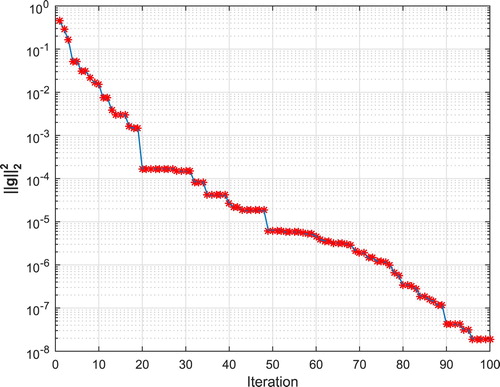
Table 7. Numerical results for Example 4.4 by using PSO method for 20 times.

k	$\Vert g(c){\Vert }_2^2$	the best solution in each run (time)
1	8.1237e−08	(1.0107, 0.9966, 0.9994, 0.9863, 1.0590)
2	5.3555e−08	(0.9940, 1.0031, 1.0005, 1.0113, 0.9546)
3	3.3184e−08	(0.9927, 1.0020, 1.0003, 1.0080, 0.9604)
4	7.8892e−09	(1.0016, 0.9989, 0.9998, 0.9959, 1.0137)
5	1.7133e−09	(0.9982, 1.0005, 1.0000, 1.0000, 0.9916)
6	6.8278e−08	(1.0000, 1.0000, 1.0000, 1.0000, 1.0002)
7	7.7655e−09	(1.0001, 1.0000, 1.0000, 0.9999, 1.0004)
8	3.0710e−04	(1.0001, 1.0000, 1.0000, 0.9998, 1.0006)
9	3.2317e−11	(1.0000, 1.0000, 1.0000, 1.0000, 1.0000)
10	6.5162e−10	(1.0000, 1.0000, 1.0000, 1.0000, 0.9999)
11	7.7656e−09	(1.0001, 1.0000, 1.0000, 0.9999, 1.0004)
12	1.3733e−08	(1.0001, 1.0000, 1.0000, 0.9999, 1.0005)
13	7.7656e−09	(1.0001, 1.0000, 1.0000, 0.9999, 1.0004)
14	7.7656e−09	(1.0001, 1.0000, 1.0000, 0.9999, 1.0004)
15	3.3378e−09	(1.0001, 1.0000, 1.0000, 0.9999, 1.0003)
16	1.9745e−08	(1.0001, 1.0000, 1.0000, 0.9999, 1.0006)
17	3.3378e−09	(1.0001, 1.0000, 1.0000, 0.9999, 1.0003)
18	5.3139e−09	(1.0000, 1.0000, 1.0000, 0.9999, 1.0003)
19	5.3139e−09	(1.0000, 1.0000, 1.0000, 0.9999, 1.0003)
20	7.7656e−09	(1.0001, 1.0000, 1.0000, 0.9999, 1.0004)

This example, demonstrate that the PSO method is very effective to find an initial guess.

5. Conclusions

In this work, two iterative methods were presented based on the Cholesky decomposition and the Jacobi method for solving some problems appeared in vibrating systems design and the design of control systems. In these methods, at first we have applied the Cholesky decomposition and rotation matrices to create a system of nonlinear equations or a constrained optimization problem and then we have solved this created system of nonlinear equations and the constrained optimization problem using Newton's method and the L-BFGS-B method, respectively. Numerical results have demonstrated the convergence of these methods and their effect for solving Problem 1.1. In addition, the second algorithm can be easily applied to parameterized generalized inverse eigenvalue problem with constrained unknown parameters. Both algorithms have used the Jacobi method, which is numerically stable and well-suited for implementation on parallel processors.

Acknowledgements

The authors are deeply grateful to the editor and anonymous referees for helpful comments and suggestions which led to a significant improvement of the original manuscript of this paper.

Disclosure statement

No potential conflict of interest was reported by the authors.

References

- Saad Y. Numerical[Q3] methods for large eigenvalue problems. Vol. 66 of 2nd revised ed. Philadelphia: SIAM; 2011.
- Güttel S, Tisseur F. The nonlinear eigenvalue problem. Acta Numer. 2017;26:1–94.
- Chu MT, Golub GH. Inverse eigenvalue problems. Oxford: Oxford University Press; 2005. (Algorithms and Applications).
- Hajarian M, Abbas H. Least squares solutions of quadratic inverse eigenvalue problem with partially bisymmetric matrices under prescribed submatrix constraints. Comput Math Appl. 2018;76(6):1458–1475.
- Hajarian M. An efficient algorithm based on Lanczos type of BCR to solve constrained quadratic inverse eigenvalue problems. J Comput Appl Math. 2019;346:418–431.
- Hajarian M. BCR algorithm for solving quadratic inverse eigenvalue problems with partially bisymmetric matrices. Asian J Control. 2020;22(2):687–695.
- Cia J, Chen J. Least-squares solutions of generalized inverse eigenvalue problem over Hermitian-Hamiltonian matrices with a submatrix constraint. Comput Appl Math. 2018;37(1):593–603.
- Liu ZY, Tan YX, Tian ZL. Generalized inverse eigenvalue problem for centrohermitian matrices. J Shanghai Univ Eng Ed. 2004;8(4):448–453.
- Gu W, Li Z. Generalized inverse eigenvalue problem for generalized snow-like matrices. Fourth International Conference on Computational and Information Sciences; 2012; Chongqing, China. IEEE. p. 662–664.
- Yuan YX, Dai H. A generalized inverse eigenvalue problem in structural dynamic model updating. J Comput Appl Math. 2009;226(1):42–49.
- Ghanbari K, Parvizpour F. Generalized inverse eigenvalue problem with mixed eigendata. Linear Algebra Appl. 2012;437(8):2056–2063.
- Gladwell GM. Inverse problems in vibration. Appl Mech Rev. 1986;39(7):1013–1018.
- Gigola S, Lebtahi L, Thome N. Inverse eigenvalue problem for normal J-hamiltonian matrices. Appl Math Lett. 2015;48:36–40.
- Chu MT, Golub GH. Structured inverse eigenvalue problems. Acta Numer. 2002;11:1–71.
- Joseph KT. Inverse eigenvalue problem in structural design. Numer Linear Algebra Appl. 1992;30(12):2890–2896.
- Jiang J, Dai H, Yuang Y. A symmetric generalized inverse eigenvalue problem in structural dynamics model updating. Linear Algebra Appl. 2013;439(5):1350–1363.
- Zhang ZZ, Han XL. Solvability conditions for algebra inverse eigenvalue problem over set of anti-Hermitian generalized anti-Hamiltonian matrices. J Cent South Univ Technol. 2005;12(1):294–297.
- Byrnes CI, Wang X. The additive inverse eigenvalue problem for Lie perturbations. SIAM J Matrix Anal Appl. 1993;14(1):113–117.
- Majkut L. Eigenvalue based inverse model of beam for structural modification and diagnostics: examples of using. Lat Am J Solids Struct. 2010;7(4):437–456.
- Cox SJ, Embree M, Hokanson JM. One can hear the composition of a string: experiments with an inverse eigenvalue problem. SIAM Rev. 2012;54(1):157–178.
- Li K, Liu J, Han J, et al. Identification of oil-film coefficients for a rotor-journal bearing system based on equivalent load reconstruction. Tribol Int. 2016;104:285–293.
- Liu J, Meng X, Zhang D, et al. An efficient method to reduce ill-posedness for structural dynamic load identification. Mech Syst Signal Process. 2017;95:273–285.
- Liu J, Sun X, Han X, et al. Dynamic load identification for stochastic structures based on gegenbauer polynomial approximation and regularization method. Mech Syst Signal Process. 2015;56:3–54.
- Bonnet M, Constantinescu A. Inverse problems in elasticity. Inverse Probl. 2005;21(2):R1.
- Barcilon V. On the multiplicity of solutions of the inverse problem for a vibrating beam. SIAM J Appl Math. 1979;37(3):605–613.
- Hasanov A, Baysal O. Identification of an unknown spatial load distribution in a vibrating cantilevered beam from final overdetermination. J Inverse Ill-posed Probl. 2015;23(1):85–102.
- Mulaik SA. Fundamentals of common factor analysis. In: The Wiley Handbook of psychometric testing: a multidisciplinary reference on survey, scale and test development. New Jersey; 2018. p. 209–251.
- Yang Y, Wei G. Inverse scattering problems for Sturm–Liouville operators with spectral parameter dependent on boundary conditions. Math Notes. 2018;103(1–2):59–66.
- Jensen JS. Phononic band gaps and vibrations in one-and two-dimensional mass–spring structures. J Sound Vib. 2003;266(5):1053–1078.
- Li LL. Sufficient conditions for the solvability of algebraic inverse eigenvalue problems. Linear Algebra Appl. 1995;221:117–129.
- Xu SF. On the sufficient conditions for the solvability of algebraic inverse eigenvalue problems. J Comput Math. 1992;10:17–80.
- Biegler-König FW. Suffcient conditions for the solubility of inverse eigenvalue problems. Linear Algebra Appl. 1981;40:89–100.
- Alexander J. The additive inverse eigenvalue problem and topological degree. Proc Amer Math Soc. 1978;70:5–7.
- Friedland S, Nocedal J, Overto ML. The formulation and analysis of numerical methods for inverse eigenvalue problems. SIAM J Numer Anal. 1987;24(3):634–667.
- Xu S. On the necessary conditions for the solvability of algebraic inverse eigenvalue problems. J Comput Math. 1992;10:93–97.
- Ji X. On matrix inverse eigenvalue problems. Inverse Probl. 1998;14(2):275–285.
- Dai H, Bai ZZ, Wei Y. On the solvability condition and numerical algorithm for the parameterized generalized inverse eigenvalue problem. SIAM J Matrix Anal Appl. 2015;36(2):707–726.
- Rojo O, Soto R. New conditions for the additive inverse eigenvalue problem for matrices. Comput Math Appl. 1992;23:41–46.
- Li L. Some sufficient conditions for the solvability of inverse eigenvalue problems. Linear Algebra Appl. 1991;148:225–236.
- Xu SF. A smallest singular value method for solving inverse eigenvalue problems. J Comput Math. 1996;1:23–31.
- Dai H. An algorithm for symmetric generalized inverse eigenvalue problems. Linear Algebra Appl. 1999;296:79–98.
- Dai H, Lancaster P. Newton's method for a generalized inverse eigenvalue problem. Numer Linear Algebra Appl. 1997;4:1–21.
- Shu L, Wang B, Hu JZ. Homotopy solution of the inverse generalized eigenvalue problems in structural dynamics. Appl Math Mech. 2004;25(5):580–586.
- Lancaster P. Algorithms for lambda-matrices. Numer Math. 1964;6(1):388–394.
- Biegler-König FW. A newton iteration process for inverse eigenvalue problems. Numer Math. 1981;37(3):349–354.
- Golub GH, VanLoan CF. Matrix computations. Vol. 3. Baltimore: JHU Press; 2012.
- Yamamoto Y, Lan Z, Kudo S. Convergence analysis of the parallel classical block Jacobi method for the symmetric eigenvalue problem. JSIAM Lett. 2014;6:57–60.
- Johnson C, Horn R. Matrix analysis. Cambridge: Cambridge university press; 1985.
- Xu D, Liu Z, Xu Y, et al. A sorted jacobi algorithm and its parallel implementation. Trans Beijing Inst Technol. 2010;12:1470–1474.
- Ji-guang S. Sensitivity analysis of multiple eigenvalues (i). Int J Comput Math. 1988;1:28–38.
- Byrd RH, Lu P, Nocedal J, et al. A limited memory algorithm for bound constrained optimization. SIAM J Sci Comput. 1995;16(5):1190–1208.
- Keskar N, Wächter A. A limited-memory quasi-newton algorithm for bound-constrained non-smooth optimization. Optim Methods Softw. 2019;34(1):150–171.
- Haarala N, Miettinen K, Mäkelä MM. Globally convergent limited memory bundle method for large-scale nonsmooth optimization. Math Program. 2007;109(1):181–205.
- Mokhtari A, Ribeiro A. Global convergence of online limited memory BFGS. J Mach Learn Res. 2015;16(1):3151–3181.
- Friedland S. Inverse eigenvalue problems. Linear Algebra Appl. 1977;17(1):15–51.
- Kennedy J, Eberhart R. Particle swarm optimization. Proceedings of the IEEE international conference on neural networks. Vol. 4; 1995. IEEE. p. 1942–1948.
- Shi Y, Eberhart R. A modified particle swarm optimizer. 1998 IEEE international conference on evolutionary computation proceedings. IEEE World Congress on Computational Intelligence (Cat. No. 98TH8360); 1998. p. 69–73.
- AlRashidi MR, El-Hawary ME. A survey of particle swarm optimization applications in electric power systems. IEEE Trans Evol Comput. 2008;13(4):913–918.
- Robinson J, Rahmat-Samii Y. Particle swarm optimization in electromagnetics. IEEE Trans Antennas Propag. 2004;52(2):397–407.
- Abousleiman R, Rawashdeh O. Electric vehicle modelling and energy-efficient routing using particle swarm optimisation. IET Intell Transp Syst. 2016;10(2):65–72.
- Gudise VG, Venayagamoorthy GK. Comparison of particle swarm optimization and backpropagation as training algorithms for neural networks. Proceedings of the 2003 IEEE Swarm Intelligence Symposium. SIS'03 (Cat. No. 03EX706); 2003; Indianapolis, USA. p. 110–117.