Reconstruction of unknown storativity and transmissivity functions in 2D groundwater equations

ABSTRACT

The paper deals with the identification from some pumping tests of unknown storativity and transmissivity functions defining a $2D$ confined aquifer. We introduce an appropriate change of variables that transforms the groundwater equation into a diffusion-reaction one wherein the diffusion term is defined by the fraction transmissivity/storativity and the reaction term yields the right hand side of a second-order nonlinear elliptic partial differential equation satisfied by the unknown storativity function. Using time records of the drawdown taken at some measuring wells within the monitored aquifer, we establish identifiability results on the involved unknown variables. We develop an identification approach that starts by determining the two auxiliary diffusion and reaction variables. Afterwards, the developed approach proposes local and global procedures to reconstruct the unknown storativity function. That leads to deduce the sought transmissivity function from the product of the two identified storativity and diffusion functions. Some numerical experiments on a variant of groundwater equations are presented.

Keywords:

• Nonlinear inverse problem
• partial differential equations: $2D$ Groundwater equations
• identification of storativity and transmissivity
• impulse response techniques and optimisation
• $2D$ confined aquifer

2010 Mathematics Subject Classification:

• 65M32

1. Introduction

Managing effectively groundwater resources requires the knowledge of some hydraulic properties defining the nature of the involved aquifers. For instance, among the main required properties we quote the following, see [1,2] Storativity: That is the volume of water released from storage with respect to the change in head (water level) and to the aquifer's surface area. Transmissivity: It represents the aquifer's ability to transmit groundwater throughout its entire saturated thickness. Since those properties affect significantly groundwater movement and storage as well as solute transport, in the literature numerous studies have been devoted to estimate such properties. Those studies are mainly based on the so-called pumping test analysis [1,3–5] which consists of analysing data, measured in some surrounding well tests, that represents the aquifer's response to a hydraulic forcing term introduced through one or multi-pumping wells. In practice, accurate estimations of the hydraulic properties lead to employ more appropriate actions in large spectrum of applications that go from groundwater exploration to waste-disposal evaluation as well as to the determination of efficiency and productivity of a well for groundwater extraction. For example, estimating transmissivity could help well field managers to design more energy-efficient pumping schemes since Sterrett reported in [6] that the energy requirement for pumping is directly proportional to the hydraulic lift. In addition, an accurate estimation of storativity is important for quantifying groundwater availability in order to satisfy drinking water demand, for instance, municipal wells in Colorado extract over 100 million cubic metres of groundwater per year.

In the literature, the identification of aquifers hydraulic properties has been initiated by Theis in [7] who used the so-called type-curve matching method to estimate aquifers parameters. Then, Cooper and Jacob employed in [8] the straight-line method to determine hydraulic properties in groundwater equations. Those techniques, called also graphical approach, are based on matching graphically the recorded data at the pumping tests to the simulations of several analytical models depending on the type of aquifers and the hydraulic conditions. In the last few decades when the use of computer became widely available, we have seen emerging several new approaches extending the graphical approach to solve applications with big data fitting and to estimate wider range of hydraulic properties as well as to explore larger class of aquifers. Those approches employ different techniques to identify the underlined hydraulic properties, for instance, stochastic techniques have been employed in [9] and genetic algorithms in [10] whereas geostatistical inversion of data by using the Bayesian approach have been used in [4,11–13] and probabilistic estiamtions using time series model in [14]. Besides, there is a direct identification approach developed in [15,16] that consists of considering the transient groundwater equation along the streamlines associated to the gradient of the drawdown as a first order ordinary differential equation of the unknown transmissivity whereas the storativity and the drawdown are both supposed to be known. Provided an initial value of the transmissivity is given for each streamline, this approach transforms the identification of the transmissivity into solving a Cauchy problem. However, the knowledge of the streamlines and of an initial transmissivity value for each streamline are difficult to achieve in the implementation of a real case. In [17], the authors introduced the so-called Differential System (DS) method that, given the drawdown for three different flows, solves the Cauchy problem in a way that doesn't require anymore the knowledge of streamlines, an initial transmissivity value is needed in only one point and no a priori knowledge of the storativity is required. Nevertheless, some remarks have been made by Beckie in [11] that the estimation of storativity is a very sensitive problem since it is influenced by the estimated transmissivity. Meier in [1] reported that the estimation of those properties in heterogeneous media depends on the measurement locations.

In the present study, we focus on identifying unknown storativity and transmissivity functions defining a $2D$ confined aquifer using some pumping tests. Based on the analysis and optimisation of the groundwater partial differential equation governing the drawdown in the considered aquifer, we develop an identification approach that uncouples the determination of the unknown storativity function from the identification of the unknown transmissivity. Moreover, the developed approach establishes conditions on the used pumping source as well as on the number and the locations of the employed measuring wells to ensure uniqueness of the involved unknown functions. The paper is organized as follows: Section 2 is devoted to introduce the problem statement and to establish some technical results for later use. In Section 3, we study the identifiability of the occurring unknown functions. Section 4, is reserved to develop the identification approach that leads to determine the unknown storativity and transmissivity functions. Some numerical experiments on a variant of groundwater equations are presented in Section 5.

2. Problem statement and technical results

Let T>0 be a finite final monitoring time and Ω be a bounded and connected open subset of $I{R}^2$ with Lipschitz boundary $\mathrm{\partial }\mathrm{\Omega }$. According to [2,7,8,18,19], it follows that due to the similarity between groundwater flow and heat conduction, the hydraulic head (water level or also called drawdown), denoted here by u, in a confined aquifer Ω subject to an external hydraulic pumping source f is governed by the following system: (1) $\{\begin{array}{ll}L[u](x_1,x_2,t)=f(x_1,x_2,t)& \mathrm{in}\mathrm{\Omega }\times (0,T)\\ u(\cdot ,0)=0& \mathrm{in}\mathrm{\Omega }\\ P\mathrm{\nabla }u\cdot \nu =0& \mathrm{on}\mathrm{\partial }\mathrm{\Omega }\times (0,T)\end{array}$(1) where ν is the unit outward vector normal to $\mathrm{\partial }\mathrm{\Omega }$ and L is the second order linear partial differential operator defined by (2) $L[u](x_1,x_2,t):=S(x_1,x_2){\mathrm{\partial }}_{t}u(x_1,x_2,t)-\mathrm{div}(P(x_1,x_2)\mathrm{\nabla }u(x_1,x_2,t))$(2) In (2(2) $L[u](x_1,x_2,t):=S(x_1,x_2){\mathrm{\partial }}_{t}u(x_1,x_2,t)-\mathrm{div}(P(x_1,x_2)\mathrm{\nabla }u(x_1,x_2,t))$(2) ), S and P designate the storativity and the transmissivity functions defining the nature of the understudy aquifer Ω. In the remainder of this paper, we consider that S and P are two differentiable functions that belong to the following admissible set: (3) $\mathcal{A}:=\{0<P\in W^{1,\mathrm{\infty }}(\mathrm{\Omega }),0<S\in W^{2,\mathrm{\infty }}(\mathrm{\Omega })\mathrm{and}S=S_0,P\mathrm{\nabla }S\cdot \nu =0\mathrm{on}\mathrm{\partial }\mathrm{\Omega }\}$(3) where $0<S_0$ is a constant number. We employ a single pumping well that reaches the aquifer at the point $a\in \mathrm{\Omega }$ through which a forcing function $\ell \in L^2(0,T)$ is pumped. Therefore, the external time-dependent pumping source f involved in (1(1) $\{\begin{array}{ll}L[u](x_1,x_2,t)=f(x_1,x_2,t)& \mathrm{in}\mathrm{\Omega }\times (0,T)\\ u(\cdot ,0)=0& \mathrm{in}\mathrm{\Omega }\\ P\mathrm{\nabla }u\cdot \nu =0& \mathrm{on}\mathrm{\partial }\mathrm{\Omega }\times (0,T)\end{array}$(1) ) is defined by (4) $f(x_1,x_2,t)=\ell (t){\delta }_a(x_1,x_2),\mathrm{for}\mathrm{all}(x_1,x_2,t)\in \mathrm{\Omega }\times (0,T)$(4) where ${\delta }_a$ denotes the Dirac mass at the pumping position a. Thus, given S and P elements of the set $\mathcal{A}$ together with $a\in \mathrm{\Omega }$ and $\ell \in L^2(0,T)$ defining f in (4(4) $f(x_1,x_2,t)=\ell (t){\delta }_a(x_1,x_2),\mathrm{for}\mathrm{all}(x_1,x_2,t)\in \mathrm{\Omega }\times (0,T)$(4) ), the forward problem (1(1) $\{\begin{array}{ll}L[u](x_1,x_2,t)=f(x_1,x_2,t)& \mathrm{in}\mathrm{\Omega }\times (0,T)\\ u(\cdot ,0)=0& \mathrm{in}\mathrm{\Omega }\\ P\mathrm{\nabla }u\cdot \nu =0& \mathrm{on}\mathrm{\partial }\mathrm{\Omega }\times (0,T)\end{array}$(1) )–(4(4) $f(x_1,x_2,t)=\ell (t){\delta }_a(x_1,x_2),\mathrm{for}\mathrm{all}(x_1,x_2,t)\in \mathrm{\Omega }\times (0,T)$(4) ) admits a unique solution u that belongs to the functional space, see [20,21]: (5) $L^2(0,T;L^2(\mathrm{\Omega }))\cap {\mathcal{C}}^0(0,T;{\left(H^1\right)}^{\mathrm{\prime }}(\mathrm{\Omega }))$(5) Moreover, the state u is sufficiently regular in $\mathrm{\Omega }\setminus \{a\}$. Therefore, given the positions of some measuring wells $b^{i=1,\dots ,\overline{I}}\in \mathrm{\Omega }\setminus \{a\}$, we define the observation operator as follows: (6) $M[S,P]:=\{u(b^i,t)\mathrm{in}(0,T),\mathrm{for}i=1,\dots ,\overline{I}\}$(6) Later on in this paper, the number $\overline{I}\in I{N}^{\ast }$ of measuring wells and their positions $b^{i=1,\dots ,\overline{I}}$ with respect to the pumping location $a\in \mathrm{\Omega }$ will be further discussed.

The nonlinear inverse problem with which we are concerned here consists of: Given time records $d_i(t)$ in $(0,T)$ of the state u taken at the measuring wells $b^{i=1,\dots ,\overline{I}}$, determine the two unknown functions S and P of $\mathcal{A}$ occurring in the problem (1(1) $\{\begin{array}{ll}L[u](x_1,x_2,t)=f(x_1,x_2,t)& \mathrm{in}\mathrm{\Omega }\times (0,T)\\ u(\cdot ,0)=0& \mathrm{in}\mathrm{\Omega }\\ P\mathrm{\nabla }u\cdot \nu =0& \mathrm{on}\mathrm{\partial }\mathrm{\Omega }\times (0,T)\end{array}$(1) )–(4(4) $f(x_1,x_2,t)=\ell (t){\delta }_a(x_1,x_2),\mathrm{for}\mathrm{all}(x_1,x_2,t)\in \mathrm{\Omega }\times (0,T)$(4) ) that yield (7) $M[S,P]=\{d_i(t)\mathrm{in}(0,T),\mathrm{for}i=1,\dots ,\overline{I}\}$(7) For later use, to each two differentiable functions S and P of the admissible set $\mathcal{A}$, we associate the intermediate variables ψ, Ψ and ρ defined as follows: (8) $\psi ={\displaystyle \frac{P}{S},\mathrm{\Psi }=\frac{1}{S}\mathrm{\nabla }S\mathrm{and}\rho =\frac{1}{4}\psi \Vert \mathrm{\Psi }{\Vert }_2^2+\frac{1}{2}\mathrm{div}\left(\psi \mathrm{\Psi }\right)}$(8) In (8(8) $\psi ={\displaystyle \frac{P}{S},\mathrm{\Psi }=\frac{1}{S}\mathrm{\nabla }S\mathrm{and}\rho =\frac{1}{4}\psi \Vert \mathrm{\Psi }{\Vert }_2^2+\frac{1}{2}\mathrm{div}\left(\psi \mathrm{\Psi }\right)}$(8) ) and in the remainder of this paper, $\Vert \cdot {\Vert }_2$ denotes the euclidean norm. Assuming the two functions ψ and ρ to be both known, it follows from (8(8) $\psi ={\displaystyle \frac{P}{S},\mathrm{\Psi }=\frac{1}{S}\mathrm{\nabla }S\mathrm{and}\rho =\frac{1}{4}\psi \Vert \mathrm{\Psi }{\Vert }_2^2+\frac{1}{2}\mathrm{div}\left(\psi \mathrm{\Psi }\right)}$(8) ) that the unknown storativity function S solves the following second order nonlinear partial differential equation: (9) $\mathrm{div}\left(\mathrm{\Psi }\right)+\frac{1}{2}\Vert \mathrm{\Psi }{\Vert }_2^2+{\displaystyle \frac{1}{\psi }\mathrm{\nabla }\psi \cdot \mathrm{\Psi }={\displaystyle \frac{2\rho }{\psi }\mathrm{in}\mathrm{\Omega }}}$(9) Besides, using the two auxiliary variables ψ and ρ introduced in (8(8) $\psi ={\displaystyle \frac{P}{S},\mathrm{\Psi }=\frac{1}{S}\mathrm{\nabla }S\mathrm{and}\rho =\frac{1}{4}\psi \Vert \mathrm{\Psi }{\Vert }_2^2+\frac{1}{2}\mathrm{div}\left(\psi \mathrm{\Psi }\right)}$(8) ), we consider the following eigenvalue problem: For all $n\in IN$, find ${\mu }_n$ and ${\xi }_n$ that solve (10) $\{\begin{array}{ll}-\mathrm{div}\left(\psi \mathrm{\nabla }{\xi }_n\right)+\rho {\xi }_n={\mu }_n{\xi }_n& \mathrm{in}\mathrm{\Omega }\\ \psi \mathrm{\nabla }{\xi }_n\cdot \nu =0& \mathrm{on}\mathrm{\partial }\mathrm{\Omega }\end{array}$(10) For the simplicity of notations, in the remainder of this paper, we denote by $\{{\xi }_n\}$ the set of normalized eigenfunctions solutions of (10(10) $\{\begin{array}{ll}-\mathrm{div}\left(\psi \mathrm{\nabla }{\xi }_n\right)+\rho {\xi }_n={\mu }_n{\xi }_n& \mathrm{in}\mathrm{\Omega }\\ \psi \mathrm{\nabla }{\xi }_n\cdot \nu =0& \mathrm{on}\mathrm{\partial }\mathrm{\Omega }\end{array}$(10) ). Since Ω is a bounded open subset of $I{R}^2$ with Lipschitz boundary $\mathrm{\partial }\mathrm{\Omega }$, it is well known that the set $\{{\xi }_n\}$ forms a complete orthonormal family of $L^2(\mathrm{\Omega })$ and their associated eigenvalues $({\mu }_n)$ form an increasing sequence of real numbers that tends to infinity, see [21]. In addition, for later use, we remind the following properties defining the principal eigenpair $({\xi }_0,{\mu }_0)$ of the problem (10(10) $\{\begin{array}{ll}-\mathrm{div}\left(\psi \mathrm{\nabla }{\xi }_n\right)+\rho {\xi }_n={\mu }_n{\xi }_n& \mathrm{in}\mathrm{\Omega }\\ \psi \mathrm{\nabla }{\xi }_n\cdot \nu =0& \mathrm{on}\mathrm{\partial }\mathrm{\Omega }\end{array}$(10) ), see [22,23]:

Remark 2.1

The principal eigenvalue ${\mu }_0$ of the problem (10(10) $\{\begin{array}{ll}-\mathrm{div}\left(\psi \mathrm{\nabla }{\xi }_n\right)+\rho {\xi }_n={\mu }_n{\xi }_n& \mathrm{in}\mathrm{\Omega }\\ \psi \mathrm{\nabla }{\xi }_n\cdot \nu =0& \mathrm{on}\mathrm{\partial }\mathrm{\Omega }\end{array}$(10) ) is of multiplicity one. Thus, it holds ${\mu }_0<{\mu }_n,\mathrm{\forall }n\in I{N}^{\ast }$. Moreover, in the case of ρ is a constant number, the principal eigenpair $({\xi }_0,{\mu }_0)$ of the problem (10(10) $\{\begin{array}{ll}-\mathrm{div}\left(\psi \mathrm{\nabla }{\xi }_n\right)+\rho {\xi }_n={\mu }_n{\xi }_n& \mathrm{in}\mathrm{\Omega }\\ \psi \mathrm{\nabla }{\xi }_n\cdot \nu =0& \mathrm{on}\mathrm{\partial }\mathrm{\Omega }\end{array}$(10) ) is defined by: ${\mu }_0=\rho$ and ${\xi }_0(x_1,x_2)=1/\sqrt{\mathcal{S}(\mathrm{\Omega })}$ for all $(x_1,x_2)\in \mathrm{\Omega }$, where $\mathcal{S}(\mathrm{\Omega })$ denotes the surface area of the domain Ω.

Furthermore, we introduce the following definition of what we will refer to later on in Corollary 3.3 as strategic point within the domain Ω:

Definition 2.2

Let $\{{\zeta }_n\}$ be a complete orthogonal family of continuous functions in $L^2(\mathrm{\Omega })$. We say that $({\hat{x}}_1,{\hat{x}}_2)\in \mathrm{\Omega }$ is strategic with respect to $\{{\zeta }_n\}$ if ${\zeta }_n({\hat{x}}_1,{\hat{x}}_2)\ne 0,\mathrm{\forall }n$.

The notion of strategic position in the sense of Definition 2.2 is well known in the literature. Indeed, this notion has been introduced by El Jai and Pritchard in [24] and used by many other authors, for example, in [25,26]. For later use, to each measuring position $b^i\in \mathrm{\Omega }\setminus \{a\}$ we associate an impulse response $G_{b^i}$ that solves: (11) $\{\begin{array}{ll}-\mathrm{div}\left(\psi \mathrm{\nabla }{G}_{b^i}\right)+\rho G_{b^i}={\displaystyle {\delta }_{b^i}(x_1,x_2)}& \mathrm{in}\mathrm{\Omega }\\ \psi \mathrm{\nabla }{G}_{b^i}\cdot \nu =0& \mathrm{on}\mathrm{\partial }\mathrm{\Omega }\end{array}$(11) Let $G_a$ be the solution of the system (11(11) $\{\begin{array}{ll}-\mathrm{div}\left(\psi \mathrm{\nabla }{G}_{b^i}\right)+\rho G_{b^i}={\displaystyle {\delta }_{b^i}(x_1,x_2)}& \mathrm{in}\mathrm{\Omega }\\ \psi \mathrm{\nabla }{G}_{b^i}\cdot \nu =0& \mathrm{on}\mathrm{\partial }\mathrm{\Omega }\end{array}$(11) ) with a instead of $b^i$. From multiplying the first equation in (11(11) $\{\begin{array}{ll}-\mathrm{div}\left(\psi \mathrm{\nabla }{G}_{b^i}\right)+\rho G_{b^i}={\displaystyle {\delta }_{b^i}(x_1,x_2)}& \mathrm{in}\mathrm{\Omega }\\ \psi \mathrm{\nabla }{G}_{b^i}\cdot \nu =0& \mathrm{on}\mathrm{\partial }\mathrm{\Omega }\end{array}$(11) ) by $G_a$ and integrating by parts over Ω using Green's formula, we obtain (12) $\begin{array}{rl}{G}_a(b^i)& =⟨-\mathrm{div}\left(\psi \mathrm{\nabla }{G}_{b^i}\right),G_a⟩+⟨\rho G_{b^i},G_a{⟩}_{L^2(\mathrm{\Omega })}\\ & =⟨-\mathrm{div}\left(\psi \mathrm{\nabla }{G}_a\right),G_{b^i}⟩+⟨\rho G_a,G_{b^i}{⟩}_{L^2(\mathrm{\Omega })}\\ & =G_{b^i}(a)\end{array}$(12) where $⟨,⟩$ represents the product in the distribution sense. The result in (12(12) $\begin{array}{rl}{G}_a(b^i)& =⟨-\mathrm{div}\left(\psi \mathrm{\nabla }{G}_{b^i}\right),G_a⟩+⟨\rho G_{b^i},G_a{⟩}_{L^2(\mathrm{\Omega })}\\ & =⟨-\mathrm{div}\left(\psi \mathrm{\nabla }{G}_a\right),G_{b^i}⟩+⟨\rho G_a,G_{b^i}{⟩}_{L^2(\mathrm{\Omega })}\\ & =G_{b^i}(a)\end{array}$(12) ) yields a symmetric property of the impulse response solution of the system (11(11) $\{\begin{array}{ll}-\mathrm{div}\left(\psi \mathrm{\nabla }{G}_{b^i}\right)+\rho G_{b^i}={\displaystyle {\delta }_{b^i}(x_1,x_2)}& \mathrm{in}\mathrm{\Omega }\\ \psi \mathrm{\nabla }{G}_{b^i}\cdot \nu =0& \mathrm{on}\mathrm{\partial }\mathrm{\Omega }\end{array}$(11) ). Moreover, using the complete orthonormal family $\{{\xi }_n\}$, the solution of (11(11) $\{\begin{array}{ll}-\mathrm{div}\left(\psi \mathrm{\nabla }{G}_{b^i}\right)+\rho G_{b^i}={\displaystyle {\delta }_{b^i}(x_1,x_2)}& \mathrm{in}\mathrm{\Omega }\\ \psi \mathrm{\nabla }{G}_{b^i}\cdot \nu =0& \mathrm{on}\mathrm{\partial }\mathrm{\Omega }\end{array}$(11) ) is given by (13) $G_{b^i}(x_1,x_2)={\displaystyle \sum _{n\ge 0}\frac{{\xi }_n(b^i)}{{\mu }_n}{\xi }_n(x_1,x_2),\mathrm{\forall }(x_1,x_2)\in \mathrm{\Omega }}$(13) Besides, as the function S fulfils 0<S in Ω, we employ the following change of variables: $U(x_1,x_2,t)=\sqrt{S(x_1,x_2)}u(x_1,x_2,t)$ in $\mathrm{\Omega }\times (0,T)$. That leads to $\mathrm{\nabla }u=S^{1/2}((1/S)\mathrm{\nabla }U-(U/2S^2)\mathrm{\nabla }S)$. Afterwards, using the intermediate variables ψ, Ψ and ρ introduced in (8(8) $\psi ={\displaystyle \frac{P}{S},\mathrm{\Psi }=\frac{1}{S}\mathrm{\nabla }S\mathrm{and}\rho =\frac{1}{4}\psi \Vert \mathrm{\Psi }{\Vert }_2^2+\frac{1}{2}\mathrm{div}\left(\psi \mathrm{\Psi }\right)}$(8) ), we get (14) $\begin{array}{rl}\mathrm{div}\left(P\mathrm{\nabla }u\right)& =\mathrm{div}\left(S^{1/2}[\psi \mathrm{\nabla }U-{\displaystyle \frac{1}{2}\psi \mathrm{\Psi }U}]\right)\\ & =S^{1/2}(\mathrm{div}\left(\psi \mathrm{\nabla }U\right)-[\frac{1}{4}\psi \Vert \mathrm{\Psi }{\Vert }_2^2+\frac{1}{2}\mathrm{div}\left(\psi \mathrm{\Psi }\right)]U)\\ & =S^{1/2}(\mathrm{div}\left(\psi \mathrm{\nabla }U\right)-\rho U)\end{array}$(14) Since in view of (3(3) $\mathcal{A}:=\{0<P\in W^{1,\mathrm{\infty }}(\mathrm{\Omega }),0<S\in W^{2,\mathrm{\infty }}(\mathrm{\Omega })\mathrm{and}S=S_0,P\mathrm{\nabla }S\cdot \nu =0\mathrm{on}\mathrm{\partial }\mathrm{\Omega }\}$(3) ) we have $P\mathrm{\nabla }S\cdot \nu =0$ on $\mathrm{\partial }\mathrm{\Omega }$, it follows that $P\mathrm{\nabla }u\cdot \nu =S^{1/2}\psi \mathrm{\nabla }U\cdot \nu$ on $\mathrm{\partial }\mathrm{\Omega }$. Hence, the problem (1(1) $\{\begin{array}{ll}L[u](x_1,x_2,t)=f(x_1,x_2,t)& \mathrm{in}\mathrm{\Omega }\times (0,T)\\ u(\cdot ,0)=0& \mathrm{in}\mathrm{\Omega }\\ P\mathrm{\nabla }u\cdot \nu =0& \mathrm{on}\mathrm{\partial }\mathrm{\Omega }\times (0,T)\end{array}$(1) )–(2(2) $L[u](x_1,x_2,t):=S(x_1,x_2){\mathrm{\partial }}_{t}u(x_1,x_2,t)-\mathrm{div}(P(x_1,x_2)\mathrm{\nabla }u(x_1,x_2,t))$(2) ) is equivalent to the following system: (15) $\{\begin{array}{ll}{\mathrm{\partial }}_{t}U-\mathrm{div}\left(\psi \mathrm{\nabla }U\right)+\rho U=S^{-1/2}f& \mathrm{in}\mathrm{\Omega }\times (0,T)\\ U(\cdot ,0)=0& \mathrm{in}\mathrm{\Omega }\\ \psi \mathrm{\nabla }U\cdot \nu =0& \mathrm{on}\mathrm{\partial }\mathrm{\Omega }\times (0,T)\end{array}$(15) Furthermore, as the set of normalized eigenfunctions $\{{\xi }_n\}$ solutions of the eigenvalue problem (10(10) $\{\begin{array}{ll}-\mathrm{div}\left(\psi \mathrm{\nabla }{\xi }_n\right)+\rho {\xi }_n={\mu }_n{\xi }_n& \mathrm{in}\mathrm{\Omega }\\ \psi \mathrm{\nabla }{\xi }_n\cdot \nu =0& \mathrm{on}\mathrm{\partial }\mathrm{\Omega }\end{array}$(10) ) forms a complete orthonormal family of $L^2(\mathrm{\Omega })$, the solution U of the system (15(15) $\{\begin{array}{ll}{\mathrm{\partial }}_{t}U-\mathrm{div}\left(\psi \mathrm{\nabla }U\right)+\rho U=S^{-1/2}f& \mathrm{in}\mathrm{\Omega }\times (0,T)\\ U(\cdot ,0)=0& \mathrm{in}\mathrm{\Omega }\\ \psi \mathrm{\nabla }U\cdot \nu =0& \mathrm{on}\mathrm{\partial }\mathrm{\Omega }\times (0,T)\end{array}$(15) ) using the pumping source f given in (4(4) $f(x_1,x_2,t)=\ell (t){\delta }_a(x_1,x_2),\mathrm{for}\mathrm{all}(x_1,x_2,t)\in \mathrm{\Omega }\times (0,T)$(4) ), can be written under the form (16) $U(x_1,x_2,t)={\displaystyle \sum _{n\ge 0}{e}_n(t){\xi }_n(x_1,x_2),\mathrm{where}\{\begin{array}{ll}{e}_n^{\mathrm{\prime }}(t)+{\mu }_n{e}_n(t)={\displaystyle \frac{{\xi }_n(a)}{\sqrt{S(a)}}}\ell (t)& \mathrm{in}(0,T)\\ e_n(0)=0& \end{array}}$(16) Therefore, from (16(16) $U(x_1,x_2,t)={\displaystyle \sum _{n\ge 0}{e}_n(t){\xi }_n(x_1,x_2),\mathrm{where}\{\begin{array}{ll}{e}_n^{\mathrm{\prime }}(t)+{\mu }_n{e}_n(t)={\displaystyle \frac{{\xi }_n(a)}{\sqrt{S(a)}}}\ell (t)& \mathrm{in}(0,T)\\ e_n(0)=0& \end{array}}$(16) ), it follows that: For all $(x_1,x_2,t)\in \mathrm{\Omega }\times (0,T)$, (17) $U(x_1,x_2,t)=\frac{1}{\sqrt{S(a)}}{\displaystyle \sum _{n\ge 0}{\xi }_n(a){\xi }_n(x_1,x_2){\int }_0^t\ell (\eta )e^{-{\mu }_n(t-\eta )}\mathrm{d}\eta }$(17) Then, for later use, we establish the following technical result that leads to express the value of the unknown storativity function S at the employed measuring wells $b^i\in \mathrm{\Omega }\setminus \{a\}$ in terms of its value at the used pumping well $a\in \mathrm{\Omega }$:

Lemma 2.3

Let $a\in \mathrm{\Omega },$ $\ell \in L^2(0,T)$ and $f(x_1,x_2,t)=\ell (t){\delta }_a(x_1,x_2)$ be the source employed in the system (1(1) $\{\begin{array}{ll}L[u](x_1,x_2,t)=f(x_1,x_2,t)& \mathrm{in}\mathrm{\Omega }\times (0,T)\\ u(\cdot ,0)=0& \mathrm{in}\mathrm{\Omega }\\ P\mathrm{\nabla }u\cdot \nu =0& \mathrm{on}\mathrm{\partial }\mathrm{\Omega }\times (0,T)\end{array}$(1) ). For all $b^i\in \mathrm{\Omega }\setminus \{a\}$ wherein the state u solution of the problem (1(1) $\{\begin{array}{ll}L[u](x_1,x_2,t)=f(x_1,x_2,t)& \mathrm{in}\mathrm{\Omega }\times (0,T)\\ u(\cdot ,0)=0& \mathrm{in}\mathrm{\Omega }\\ P\mathrm{\nabla }u\cdot \nu =0& \mathrm{on}\mathrm{\partial }\mathrm{\Omega }\times (0,T)\end{array}$(1) )–(3(3) $\mathcal{A}:=\{0<P\in W^{1,\mathrm{\infty }}(\mathrm{\Omega }),0<S\in W^{2,\mathrm{\infty }}(\mathrm{\Omega })\mathrm{and}S=S_0,P\mathrm{\nabla }S\cdot \nu =0\mathrm{on}\mathrm{\partial }\mathrm{\Omega }\}$(3) ) yields ${\int }_0^{T}u(b^i,t)\mathrm{d}t\ne 0,$ the unknown function S occurring in (1(1) $\{\begin{array}{ll}L[u](x_1,x_2,t)=f(x_1,x_2,t)& \mathrm{in}\mathrm{\Omega }\times (0,T)\\ u(\cdot ,0)=0& \mathrm{in}\mathrm{\Omega }\\ P\mathrm{\nabla }u\cdot \nu =0& \mathrm{on}\mathrm{\partial }\mathrm{\Omega }\times (0,T)\end{array}$(1) )–(3(3) $\mathcal{A}:=\{0<P\in W^{1,\mathrm{\infty }}(\mathrm{\Omega }),0<S\in W^{2,\mathrm{\infty }}(\mathrm{\Omega })\mathrm{and}S=S_0,P\mathrm{\nabla }S\cdot \nu =0\mathrm{on}\mathrm{\partial }\mathrm{\Omega }\}$(3) ) is subject to: (18) ${\displaystyle \sqrt{S(b^i)}={\displaystyle \frac{1}{\sqrt{S(a)}}{B}^i}}$(18) where the coefficient $B^i$ is given by (19) $B^i={\displaystyle \frac{{\displaystyle \sum _{n\ge 0}\frac{{\xi }_n(a){\xi }_n(b^i)}{{\mu }_n}{\displaystyle {\int }_0^T\ell (t)(1-e^{-{\mu }_n(T-t)})\mathrm{d}t}}}{{\displaystyle {\int }_0^{T}u(b^i,t)\mathrm{d}t}}}$(19) In (19(19) $B^i={\displaystyle \frac{{\displaystyle \sum _{n\ge 0}\frac{{\xi }_n(a){\xi }_n(b^i)}{{\mu }_n}{\displaystyle {\int }_0^T\ell (t)(1-e^{-{\mu }_n(T-t)})\mathrm{d}t}}}{{\displaystyle {\int }_0^{T}u(b^i,t)\mathrm{d}t}}}$(19) ), $({\xi }_n,{\mu }_n)$ are the eigenpairs solutions of the eigenvalue problem (10(10) $\{\begin{array}{ll}-\mathrm{div}\left(\psi \mathrm{\nabla }{\xi }_n\right)+\rho {\xi }_n={\mu }_n{\xi }_n& \mathrm{in}\mathrm{\Omega }\\ \psi \mathrm{\nabla }{\xi }_n\cdot \nu =0& \mathrm{on}\mathrm{\partial }\mathrm{\Omega }\end{array}$(10) ).

Proof.

Let $b^i\in \mathrm{\Omega }\setminus \{a\}$ and $G_{b^i}$ be the solution of the system (11(11) $\{\begin{array}{ll}-\mathrm{div}\left(\psi \mathrm{\nabla }{G}_{b^i}\right)+\rho G_{b^i}={\displaystyle {\delta }_{b^i}(x_1,x_2)}& \mathrm{in}\mathrm{\Omega }\\ \psi \mathrm{\nabla }{G}_{b^i}\cdot \nu =0& \mathrm{on}\mathrm{\partial }\mathrm{\Omega }\end{array}$(11) ). From multiplying the first equation of this system by U the solution of the problem (15(15) $\{\begin{array}{ll}{\mathrm{\partial }}_{t}U-\mathrm{div}\left(\psi \mathrm{\nabla }U\right)+\rho U=S^{-1/2}f& \mathrm{in}\mathrm{\Omega }\times (0,T)\\ U(\cdot ,0)=0& \mathrm{in}\mathrm{\Omega }\\ \psi \mathrm{\nabla }U\cdot \nu =0& \mathrm{on}\mathrm{\partial }\mathrm{\Omega }\times (0,T)\end{array}$(15) ), where f is given in (4(4) $f(x_1,x_2,t)=\ell (t){\delta }_a(x_1,x_2),\mathrm{for}\mathrm{all}(x_1,x_2,t)\in \mathrm{\Omega }\times (0,T)$(4) ), and integrating by parts over Ω using Green's formula, we get: For all $t\in (0,T)$, (20) $\begin{array}{rl}U(b^i,t)& ={\displaystyle ⟨-\mathrm{div}(\psi \mathrm{\nabla }U),G_{b^i}⟩+⟨\rho U,G_{b^i}{⟩}_{L^2(\mathrm{\Omega })}}\\ & ={\displaystyle \frac{G_{b^i}(a)}{\sqrt{S(a)}}\ell (t)-\frac{\mathrm{d}}{\mathrm{d}t}⟨U,G_{b^i}{⟩}_{L^2(\mathrm{\Omega })}}\end{array}$(20) where $⟨,⟩$ is the product in the distribution sense. Since $U(b^i,t)=\sqrt{S(b^i)}u(b^i,t)$, for all $t\in (0,T)$ and $U(\cdot ,0)=0$ in Ω, it follows from integrating (20(20) $\begin{array}{rl}U(b^i,t)& ={\displaystyle ⟨-\mathrm{div}(\psi \mathrm{\nabla }U),G_{b^i}⟩+⟨\rho U,G_{b^i}{⟩}_{L^2(\mathrm{\Omega })}}\\ & ={\displaystyle \frac{G_{b^i}(a)}{\sqrt{S(a)}}\ell (t)-\frac{\mathrm{d}}{\mathrm{d}t}⟨U,G_{b^i}{⟩}_{L^2(\mathrm{\Omega })}}\end{array}$(20) ) over $(0,T)$ that (21) $\sqrt{S(b^i)}={\displaystyle \frac{{\displaystyle \frac{G_{b^i}(a)}{\sqrt{S(a)}}{\displaystyle {\int }_0^T\ell (t)dt-⟨U(\cdot ,T),G_{b^i}{⟩}_{L^2(\mathrm{\Omega })}}}}{{\displaystyle {\int }_0^{T}u(b^i,t)\mathrm{d}t}}}$(21) Besides, as the set $\{{\xi }_n\}$ forms a complete orthonormal family of $L^2(\mathrm{\Omega })$ then, from using the result in (17(17) $U(x_1,x_2,t)=\frac{1}{\sqrt{S(a)}}{\displaystyle \sum _{n\ge 0}{\xi }_n(a){\xi }_n(x_1,x_2){\int }_0^t\ell (\eta )e^{-{\mu }_n(t-\eta )}\mathrm{d}\eta }$(17) ) to compute $U(\cdot ,T)$ and replacing the impulse response $G_{b^i}$ by its value given in (13(13) $G_{b^i}(x_1,x_2)={\displaystyle \sum _{n\ge 0}\frac{{\xi }_n(b^i)}{{\mu }_n}{\xi }_n(x_1,x_2),\mathrm{\forall }(x_1,x_2)\in \mathrm{\Omega }}$(13) ), we obtain (22) $\begin{array}{rl}⟨U(\cdot ,T),G_{b^i}{⟩}_{L^2(\mathrm{\Omega })}& ={\displaystyle \frac{1}{\sqrt{S(a)}}{⟨{\displaystyle \sum _{n\ge 0}{\xi }_n(a){\displaystyle {\int }_0^T\ell (t)e^{-{\mu }_n(T-t)}\mathrm{d}t{\xi }_n,{\displaystyle \sum _{k\ge 0}\frac{{\xi }_k(b^i)}{{\mu }_k}{\xi }_k}}}⟩}_{L^2(\mathrm{\Omega })}}\\ & ={\displaystyle \frac{1}{\sqrt{S(a)}}{\displaystyle \sum _{n\ge 0}\frac{{\xi }_n(a){\xi }_n(b^i)}{{\mu }_n}{\displaystyle {\int }_0^T\ell (t)e^{-{\mu }_n(T-t)}\mathrm{d}t}}}\end{array}$(22) Afterwards, substituting in (21(21) $\sqrt{S(b^i)}={\displaystyle \frac{{\displaystyle \frac{G_{b^i}(a)}{\sqrt{S(a)}}{\displaystyle {\int }_0^T\ell (t)dt-⟨U(\cdot ,T),G_{b^i}{⟩}_{L^2(\mathrm{\Omega })}}}}{{\displaystyle {\int }_0^{T}u(b^i,t)\mathrm{d}t}}}$(21) ) the terms $⟨U(\cdot ,T),G_{b^i}{⟩}_{L^2(\mathrm{\Omega })}$ by its value obtained in (22(22) $\begin{array}{rl}⟨U(\cdot ,T),G_{b^i}{⟩}_{L^2(\mathrm{\Omega })}& ={\displaystyle \frac{1}{\sqrt{S(a)}}{⟨{\displaystyle \sum _{n\ge 0}{\xi }_n(a){\displaystyle {\int }_0^T\ell (t)e^{-{\mu }_n(T-t)}\mathrm{d}t{\xi }_n,{\displaystyle \sum _{k\ge 0}\frac{{\xi }_k(b^i)}{{\mu }_k}{\xi }_k}}}⟩}_{L^2(\mathrm{\Omega })}}\\ & ={\displaystyle \frac{1}{\sqrt{S(a)}}{\displaystyle \sum _{n\ge 0}\frac{{\xi }_n(a){\xi }_n(b^i)}{{\mu }_n}{\displaystyle {\int }_0^T\ell (t)e^{-{\mu }_n(T-t)}\mathrm{d}t}}}\end{array}$(22) ) and $G_{b^i}(a)$ by its value deduced from (13(13) $G_{b^i}(x_1,x_2)={\displaystyle \sum _{n\ge 0}\frac{{\xi }_n(b^i)}{{\mu }_n}{\xi }_n(x_1,x_2),\mathrm{\forall }(x_1,x_2)\in \mathrm{\Omega }}$(13) ) leads to the result announced in (18(18) ${\displaystyle \sqrt{S(b^i)}={\displaystyle \frac{1}{\sqrt{S(a)}}{B}^i}}$(18) )–(19(19) $B^i={\displaystyle \frac{{\displaystyle \sum _{n\ge 0}\frac{{\xi }_n(a){\xi }_n(b^i)}{{\mu }_n}{\displaystyle {\int }_0^T\ell (t)(1-e^{-{\mu }_n(T-t)})\mathrm{d}t}}}{{\displaystyle {\int }_0^{T}u(b^i,t)\mathrm{d}t}}}$(19) ).

Since $u(x_1,x_2,t)=U(x_1,x_2,t)/\sqrt{S(x_1,x_2)}$ for all $(x_1,x_2,t)\in \mathrm{\Omega }\times (0,T)$, it follows from (17(17) $U(x_1,x_2,t)=\frac{1}{\sqrt{S(a)}}{\displaystyle \sum _{n\ge 0}{\xi }_n(a){\xi }_n(x_1,x_2){\int }_0^t\ell (\eta )e^{-{\mu }_n(t-\eta )}\mathrm{d}\eta }$(17) ) that: For all measuring well $b^i\in \mathrm{\Omega }\setminus \{a\}$ wherein Lemma 2.3 applies, the state u solution of the problem (1(1) $\{\begin{array}{ll}L[u](x_1,x_2,t)=f(x_1,x_2,t)& \mathrm{in}\mathrm{\Omega }\times (0,T)\\ u(\cdot ,0)=0& \mathrm{in}\mathrm{\Omega }\\ P\mathrm{\nabla }u\cdot \nu =0& \mathrm{on}\mathrm{\partial }\mathrm{\Omega }\times (0,T)\end{array}$(1) )–(4(4) $f(x_1,x_2,t)=\ell (t){\delta }_a(x_1,x_2),\mathrm{for}\mathrm{all}(x_1,x_2,t)\in \mathrm{\Omega }\times (0,T)$(4) ) taken at $b^i$ is given by (23) $u(b^i,t)={\displaystyle \frac{1}{B^i}\sum _{n\ge 0}{\xi }_n(a){\xi }_n(b^i){\displaystyle {\int }_0^t\ell (\eta )e^{-{\mu }_n(t-\eta )}\mathrm{d}\eta ,\mathrm{\forall }t\in (0,T)}}$(23) where $B^i$ is the coefficient in (19(19) $B^i={\displaystyle \frac{{\displaystyle \sum _{n\ge 0}\frac{{\xi }_n(a){\xi }_n(b^i)}{{\mu }_n}{\displaystyle {\int }_0^T\ell (t)(1-e^{-{\mu }_n(T-t)})\mathrm{d}t}}}{{\displaystyle {\int }_0^{T}u(b^i,t)\mathrm{d}t}}}$(19) ) and $({\xi }_n,{\mu }_n)$ are the eigenpairs solutions of the problem (10(10) $\{\begin{array}{ll}-\mathrm{div}\left(\psi \mathrm{\nabla }{\xi }_n\right)+\rho {\xi }_n={\mu }_n{\xi }_n& \mathrm{in}\mathrm{\Omega }\\ \psi \mathrm{\nabla }{\xi }_n\cdot \nu =0& \mathrm{on}\mathrm{\partial }\mathrm{\Omega }\end{array}$(10) ). Therefore, given time records $d_i(t)$ in $(0,T)$ of the state u solution of the system (1(1) $\{\begin{array}{ll}L[u](x_1,x_2,t)=f(x_1,x_2,t)& \mathrm{in}\mathrm{\Omega }\times (0,T)\\ u(\cdot ,0)=0& \mathrm{in}\mathrm{\Omega }\\ P\mathrm{\nabla }u\cdot \nu =0& \mathrm{on}\mathrm{\partial }\mathrm{\Omega }\times (0,T)\end{array}$(1) )–(4(4) $f(x_1,x_2,t)=\ell (t){\delta }_a(x_1,x_2),\mathrm{for}\mathrm{all}(x_1,x_2,t)\in \mathrm{\Omega }\times (0,T)$(4) ) at such a measuring well $b^i\in \mathrm{\Omega }\setminus \{a\}$, we can determine the two auxiliary variables ψ and ρ occurring in the problem (10(10) $\{\begin{array}{ll}-\mathrm{div}\left(\psi \mathrm{\nabla }{\xi }_n\right)+\rho {\xi }_n={\mu }_n{\xi }_n& \mathrm{in}\mathrm{\Omega }\\ \psi \mathrm{\nabla }{\xi }_n\cdot \nu =0& \mathrm{on}\mathrm{\partial }\mathrm{\Omega }\end{array}$(10) ) that lead $u(b^i,\cdot )$ in (23(23) $u(b^i,t)={\displaystyle \frac{1}{B^i}\sum _{n\ge 0}{\xi }_n(a){\xi }_n(b^i){\displaystyle {\int }_0^t\ell (\eta )e^{-{\mu }_n(t-\eta )}\mathrm{d}\eta ,\mathrm{\forall }t\in (0,T)}}$(23) ) to match the measurements $d_i(\cdot )$. Moreover, since $({\mu }_n)$ is an increasing sequence that tends to $+\mathrm{\infty }$, one could truncate the series in (23(23) $u(b^i,t)={\displaystyle \frac{1}{B^i}\sum _{n\ge 0}{\xi }_n(a){\xi }_n(b^i){\displaystyle {\int }_0^t\ell (\eta )e^{-{\mu }_n(t-\eta )}\mathrm{d}\eta ,\mathrm{\forall }t\in (0,T)}}$(23) ) using a sufficiently large number $N\in I{N}^{\ast }$ of first terms and solve: (24) ${\displaystyle \underset{\psi ,\rho }{min}{\displaystyle \sum _{i=1}^I{\mathcal{R}}_i^N(\psi ,\rho )\text{subject to:}\psi >0\mathrm{in}\mathrm{\Omega }}}$(24) where I is the number of measuring wells $b^i$ wherein Lemma 2.3 applies and (25) ${\mathcal{R}}_i^N(\psi ,\rho )=\frac{1}{2}{\Vert {\displaystyle \frac{1}{B^i}\sum _{n=0}^N{\xi }_n(a){\xi }_n(b^i){\displaystyle {\int }_0^t\ell (\eta )e^{-{\mu }_n(t-\eta )}\mathrm{d}\eta -d_i(t)}}\Vert }_{L^2(0,T)}^2$(25) Then, using the solutions ψ and ρ of the minimisation problem (24(24) ${\displaystyle \underset{\psi ,\rho }{min}{\displaystyle \sum _{i=1}^I{\mathcal{R}}_i^N(\psi ,\rho )\text{subject to:}\psi >0\mathrm{in}\mathrm{\Omega }}}$(24) )–(25(25) ${\mathcal{R}}_i^N(\psi ,\rho )=\frac{1}{2}{\Vert {\displaystyle \frac{1}{B^i}\sum _{n=0}^N{\xi }_n(a){\xi }_n(b^i){\displaystyle {\int }_0^t\ell (\eta )e^{-{\mu }_n(t-\eta )}\mathrm{d}\eta -d_i(t)}}\Vert }_{L^2(0,T)}^2$(25) ), it follows that the two unknown functions S and P occurring in the system (1(1) $\{\begin{array}{ll}L[u](x_1,x_2,t)=f(x_1,x_2,t)& \mathrm{in}\mathrm{\Omega }\times (0,T)\\ u(\cdot ,0)=0& \mathrm{in}\mathrm{\Omega }\\ P\mathrm{\nabla }u\cdot \nu =0& \mathrm{on}\mathrm{\partial }\mathrm{\Omega }\times (0,T)\end{array}$(1) )–(4(4) $f(x_1,x_2,t)=\ell (t){\delta }_a(x_1,x_2),\mathrm{for}\mathrm{all}(x_1,x_2,t)\in \mathrm{\Omega }\times (0,T)$(4) ) are subject to (8(8) $\psi ={\displaystyle \frac{P}{S},\mathrm{\Psi }=\frac{1}{S}\mathrm{\nabla }S\mathrm{and}\rho =\frac{1}{4}\psi \Vert \mathrm{\Psi }{\Vert }_2^2+\frac{1}{2}\mathrm{div}\left(\psi \mathrm{\Psi }\right)}$(8) )–(9(9) $\mathrm{div}\left(\mathrm{\Psi }\right)+\frac{1}{2}\Vert \mathrm{\Psi }{\Vert }_2^2+{\displaystyle \frac{1}{\psi }\mathrm{\nabla }\psi \cdot \mathrm{\Psi }={\displaystyle \frac{2\rho }{\psi }\mathrm{in}\mathrm{\Omega }}}$(9) ). In addition, according to (18(18) ${\displaystyle \sqrt{S(b^i)}={\displaystyle \frac{1}{\sqrt{S(a)}}{B}^i}}$(18) ), the unknown function S is also subject to: (26) $S(a)S(b^i)={\left(B^i\right)}^2,\mathrm{for}i=1,\dots ,I$(26) where $B^i$ is the coefficient in (19(19) $B^i={\displaystyle \frac{{\displaystyle \sum _{n\ge 0}\frac{{\xi }_n(a){\xi }_n(b^i)}{{\mu }_n}{\displaystyle {\int }_0^T\ell (t)(1-e^{-{\mu }_n(T-t)})\mathrm{d}t}}}{{\displaystyle {\int }_0^{T}u(b^i,t)\mathrm{d}t}}}$(19) ) computed from the solutions ψ and ρ of (24(24) ${\displaystyle \underset{\psi ,\rho }{min}{\displaystyle \sum _{i=1}^I{\mathcal{R}}_i^N(\psi ,\rho )\text{subject to:}\psi >0\mathrm{in}\mathrm{\Omega }}}$(24) )–(25(25) ${\mathcal{R}}_i^N(\psi ,\rho )=\frac{1}{2}{\Vert {\displaystyle \frac{1}{B^i}\sum _{n=0}^N{\xi }_n(a){\xi }_n(b^i){\displaystyle {\int }_0^t\ell (\eta )e^{-{\mu }_n(t-\eta )}\mathrm{d}\eta -d_i(t)}}\Vert }_{L^2(0,T)}^2$(25) ).

Remark 2.4

The identification approach developed in this paper consists of determining the two auxiliary variables ψ and ρ from solving the minimisation problem (24(24) ${\displaystyle \underset{\psi ,\rho }{min}{\displaystyle \sum _{i=1}^I{\mathcal{R}}_i^N(\psi ,\rho )\text{subject to:}\psi >0\mathrm{in}\mathrm{\Omega }}}$(24) )–(25(25) ${\mathcal{R}}_i^N(\psi ,\rho )=\frac{1}{2}{\Vert {\displaystyle \frac{1}{B^i}\sum _{n=0}^N{\xi }_n(a){\xi }_n(b^i){\displaystyle {\int }_0^t\ell (\eta )e^{-{\mu }_n(t-\eta )}\mathrm{d}\eta -d_i(t)}}\Vert }_{L^2(0,T)}^2$(25) ) and then, deducing the unknown functions S and P subject to (8(8) $\psi ={\displaystyle \frac{P}{S},\mathrm{\Psi }=\frac{1}{S}\mathrm{\nabla }S\mathrm{and}\rho =\frac{1}{4}\psi \Vert \mathrm{\Psi }{\Vert }_2^2+\frac{1}{2}\mathrm{div}\left(\psi \mathrm{\Psi }\right)}$(8) )–(9(9) $\mathrm{div}\left(\mathrm{\Psi }\right)+\frac{1}{2}\Vert \mathrm{\Psi }{\Vert }_2^2+{\displaystyle \frac{1}{\psi }\mathrm{\nabla }\psi \cdot \mathrm{\Psi }={\displaystyle \frac{2\rho }{\psi }\mathrm{in}\mathrm{\Omega }}}$(9) ) and (26(26) $S(a)S(b^i)={\left(B^i\right)}^2,\mathrm{for}i=1,\dots ,I$(26) ). Among the main advantages of the developed approach, we have: (1) In terms of optimisation cost, the minimisation of the problem (24(24) ${\displaystyle \underset{\psi ,\rho }{min}{\displaystyle \sum _{i=1}^I{\mathcal{R}}_i^N(\psi ,\rho )\text{subject to:}\psi >0\mathrm{in}\mathrm{\Omega }}}$(24) )–(25(25) ${\mathcal{R}}_i^N(\psi ,\rho )=\frac{1}{2}{\Vert {\displaystyle \frac{1}{B^i}\sum _{n=0}^N{\xi }_n(a){\xi }_n(b^i){\displaystyle {\int }_0^t\ell (\eta )e^{-{\mu }_n(t-\eta )}\mathrm{d}\eta -d_i(t)}}\Vert }_{L^2(0,T)}^2$(25) ) does not require solving any time-dependent partial differential equation. Moreover, for example, in the case of ψ, ρ are two constant numbers and Ω is of a classic geometry shape, the eigenpairs $({\xi }_n,{\mu }_n)$ solutions of (10(10) $\{\begin{array}{ll}-\mathrm{div}\left(\psi \mathrm{\nabla }{\xi }_n\right)+\rho {\xi }_n={\mu }_n{\xi }_n& \mathrm{in}\mathrm{\Omega }\\ \psi \mathrm{\nabla }{\xi }_n\cdot \nu =0& \mathrm{on}\mathrm{\partial }\mathrm{\Omega }\end{array}$(10) ) can be given explicitly. (2) In terms of stability, we identify diffusion and reaction variables that are associated with even derivative orders of the corresponding state ${\xi }_n$.

In the sequel, from the observation operator $M[S,P]$ introduced in (6(6) $M[S,P]:=\{u(b^i,t)\mathrm{in}(0,T),\mathrm{for}i=1,\dots ,\overline{I}\}$(6) ), we establish identifiability results on the involved unknown variables and develop an identification method that leads to determine the unknowns S and P occurring in the problem (1(1) $\{\begin{array}{ll}L[u](x_1,x_2,t)=f(x_1,x_2,t)& \mathrm{in}\mathrm{\Omega }\times (0,T)\\ u(\cdot ,0)=0& \mathrm{in}\mathrm{\Omega }\\ P\mathrm{\nabla }u\cdot \nu =0& \mathrm{on}\mathrm{\partial }\mathrm{\Omega }\times (0,T)\end{array}$(1) )–(4(4) $f(x_1,x_2,t)=\ell (t){\delta }_a(x_1,x_2),\mathrm{for}\mathrm{all}(x_1,x_2,t)\in \mathrm{\Omega }\times (0,T)$(4) ).

3. Identifiability

We start this section by establishing that under some regularity assumptions, the knowledge of the two auxiliary variables ψ and ρ along with a constant number $B^i$ fulfiling one equation of (26(26) $S(a)S(b^i)={\left(B^i\right)}^2,\mathrm{for}i=1,\dots ,I$(26) ) determines in a unique manner the unknown function S subject to (9(9) $\mathrm{div}\left(\mathrm{\Psi }\right)+\frac{1}{2}\Vert \mathrm{\Psi }{\Vert }_2^2+{\displaystyle \frac{1}{\psi }\mathrm{\nabla }\psi \cdot \mathrm{\Psi }={\displaystyle \frac{2\rho }{\psi }\mathrm{in}\mathrm{\Omega }}}$(9) ). Afterwards, the second unknown function P is then deduced from S and ψ as in (8(8) $\psi ={\displaystyle \frac{P}{S},\mathrm{\Psi }=\frac{1}{S}\mathrm{\nabla }S\mathrm{and}\rho =\frac{1}{4}\psi \Vert \mathrm{\Psi }{\Vert }_2^2+\frac{1}{2}\mathrm{div}\left(\psi \mathrm{\Psi }\right)}$(8) ).

Theorem 3.1

Let $a\in \mathrm{\Omega }$ and $b^i\in \mathrm{\Omega }\setminus \{a\}$. Given a constant number $B^i$ and two functions ψ and ρ such that (27) ${\Vert \frac{1}{\psi }\mathrm{\nabla }\psi \Vert }_2\in L^{\mathrm{\infty }}(\mathrm{\Omega })and\frac{\rho }{\psi }\in L^{\gamma }(\mathrm{\Omega }),forsome\gamma >1$(27) there exists a unique function S of the form $S=S_0{e}^{-G}$ in Ω that solves the equation (9(9) $\mathrm{div}\left(\mathrm{\Psi }\right)+\frac{1}{2}\Vert \mathrm{\Psi }{\Vert }_2^2+{\displaystyle \frac{1}{\psi }\mathrm{\nabla }\psi \cdot \mathrm{\Psi }={\displaystyle \frac{2\rho }{\psi }\mathrm{in}\mathrm{\Omega }}}$(9) ), yields $S(a)S(b^i)=(B^i{)}^2$ and satisfies the boundary condition $S=S_0$ on $\mathrm{\partial }\mathrm{\Omega },$ where $0<S_0$ is a constant number and the function $G\in H_0^1(\mathrm{\Omega })\cap L^{\mathrm{\infty }}(\mathrm{\Omega })$.

Proof.

For k = 1, 2, let $S^{(k)}=S_0^{(k)}{e}^{-G^{(k)}}$ in Ω be a solution of the equation (9(9) $\mathrm{div}\left(\mathrm{\Psi }\right)+\frac{1}{2}\Vert \mathrm{\Psi }{\Vert }_2^2+{\displaystyle \frac{1}{\psi }\mathrm{\nabla }\psi \cdot \mathrm{\Psi }={\displaystyle \frac{2\rho }{\psi }\mathrm{in}\mathrm{\Omega }}}$(9) ) that satisfies $S^{(k)}=S_0^{(k)}$ on $\mathrm{\partial }\mathrm{\Omega }$, where $0<S_0^{(k)}$ is a constant number. That implies the variable ${\mathrm{\Psi }}^{(k)}=(1/S^{(k)})\mathrm{\nabla }{S}^{(k)}$ is given by ${\mathrm{\Psi }}^{(k)}=-\mathrm{\nabla }{G}^{(k)}$ in Ω. Afterwards, in view of (9(9) $\mathrm{div}\left(\mathrm{\Psi }\right)+\frac{1}{2}\Vert \mathrm{\Psi }{\Vert }_2^2+{\displaystyle \frac{1}{\psi }\mathrm{\nabla }\psi \cdot \mathrm{\Psi }={\displaystyle \frac{2\rho }{\psi }\mathrm{in}\mathrm{\Omega }}}$(9) ), it follows that the two functions $G^{(k=1,2)}$ solve the following system: (28) $\{\begin{array}{ll}-\mathrm{\Delta }{G}^{(k)}+{\displaystyle \frac{1}{2}}{\Vert \mathrm{\nabla }{G}^{(k)}\Vert }_2^2-{\displaystyle \frac{1}{\psi }\mathrm{\nabla }\psi \cdot \mathrm{\nabla }{G}^{(k)}=2{\displaystyle \frac{\rho }{\psi }}}& \mathrm{in}\mathrm{\Omega }\\ G^{(k)}=0& \mathrm{on}\mathrm{\partial }\mathrm{\Omega }\end{array}$(28) Moreover, from referring to Theorem 2.2 in [27], it comes that the problem (28(28) $\{\begin{array}{ll}-\mathrm{\Delta }{G}^{(k)}+{\displaystyle \frac{1}{2}}{\Vert \mathrm{\nabla }{G}^{(k)}\Vert }_2^2-{\displaystyle \frac{1}{\psi }\mathrm{\nabla }\psi \cdot \mathrm{\nabla }{G}^{(k)}=2{\displaystyle \frac{\rho }{\psi }}}& \mathrm{in}\mathrm{\Omega }\\ G^{(k)}=0& \mathrm{on}\mathrm{\partial }\mathrm{\Omega }\end{array}$(28) ) admits at most one solution which belongs to $H_0^1(\mathrm{\Omega })\cap L^{\mathrm{\infty }}(\mathrm{\Omega })$. That leads to $G^{(2)}=G^{(1)}$ in Ω. Furthermore, since the two functions $S^{(1)}$ and $S^{(2)}$ fulfil $S^{(1)}(a)S^{(1)}(b^i)=(B^i{)}^2=S^{(2)}(a)S^{(2)}(b^i)$, it follows that $S_0^{(2)}=S_0^{(1)}$. Therefore, we obtain $S^{(2)}=S^{(1)}$ in Ω.

Besides, regarding the determination of the two auxiliary variables ψ and ρ as well as of the constant numbers $S(a)S(b^i)$ at the employed measuring wells $b^i\in \mathrm{\Omega }\setminus \{a\}$, we start by proving that in the case of ψ and ρ are two constant numbers, the observation operator $M[S,P]$ introduced in (6(6) $M[S,P]:=\{u(b^i,t)\mathrm{in}(0,T),\mathrm{for}i=1,\dots ,\overline{I}\}$(6) ) yields identifiability of those unknowns.

Theorem 3.2

Let $\ell \in L^2(0,T)$ be such that $\ell (t)\ne 0$ a.e. in $(0,T),$ $a\in \mathrm{\Omega }$, $I\in I{N}^{\ast }$ and $b^i\in \mathrm{\Omega }\setminus \{a\},$ for $i=1,\dots ,I$. Provided ψ and ρ occurring in (8(8) $\psi ={\displaystyle \frac{P}{S},\mathrm{\Psi }=\frac{1}{S}\mathrm{\nabla }S\mathrm{and}\rho =\frac{1}{4}\psi \Vert \mathrm{\Psi }{\Vert }_2^2+\frac{1}{2}\mathrm{div}\left(\psi \mathrm{\Psi }\right)}$(8) )–(9(9) $\mathrm{div}\left(\mathrm{\Psi }\right)+\frac{1}{2}\Vert \mathrm{\Psi }{\Vert }_2^2+{\displaystyle \frac{1}{\psi }\mathrm{\nabla }\psi \cdot \mathrm{\Psi }={\displaystyle \frac{2\rho }{\psi }\mathrm{in}\mathrm{\Omega }}}$(9) ) are two constant numbers and the second eigenpair $({\xi }_1,{\mu }_1)$ of the eigenvalue problem (10(10) $\{\begin{array}{ll}-\mathrm{div}\left(\psi \mathrm{\nabla }{\xi }_n\right)+\rho {\xi }_n={\mu }_n{\xi }_n& \mathrm{in}\mathrm{\Omega }\\ \psi \mathrm{\nabla }{\xi }_n\cdot \nu =0& \mathrm{on}\mathrm{\partial }\mathrm{\Omega }\end{array}$(10) ) satisfies

1. The eigenvalue ${\mu }_1$ is of multiplicity equal to 1.

2. There exists $i_0\in \{1,\dots ,I\}$ such that ${\xi }_1(a){\xi }_1(b^{i_0})\ne 0$.

the observation operator $M[S,P]$ determines uniquely ψ, ρ and $S(a)S(b^i),$ for $i=1,\dots ,I$.

Proof.

For k = 1, 2, let $S^{(k)}$ and $P^{(k)}$ be elements of the admissible set (3(3) $\mathcal{A}:=\{0<P\in W^{1,\mathrm{\infty }}(\mathrm{\Omega }),0<S\in W^{2,\mathrm{\infty }}(\mathrm{\Omega })\mathrm{and}S=S_0,P\mathrm{\nabla }S\cdot \nu =0\mathrm{on}\mathrm{\partial }\mathrm{\Omega }\}$(3) ) such that ${\psi }^{(k)}$ and ${\rho }^{(k)}$ defined in (8(8) $\psi ={\displaystyle \frac{P}{S},\mathrm{\Psi }=\frac{1}{S}\mathrm{\nabla }S\mathrm{and}\rho =\frac{1}{4}\psi \Vert \mathrm{\Psi }{\Vert }_2^2+\frac{1}{2}\mathrm{div}\left(\psi \mathrm{\Psi }\right)}$(8) ) from $S^{(k)}$, $P^{(k)}$ instead of S, P are two constant numbers. We denote by $u^{(k)}$ the solution of the system (1(1) $\{\begin{array}{ll}L[u](x_1,x_2,t)=f(x_1,x_2,t)& \mathrm{in}\mathrm{\Omega }\times (0,T)\\ u(\cdot ,0)=0& \mathrm{in}\mathrm{\Omega }\\ P\mathrm{\nabla }u\cdot \nu =0& \mathrm{on}\mathrm{\partial }\mathrm{\Omega }\times (0,T)\end{array}$(1) )–(4(4) $f(x_1,x_2,t)=\ell (t){\delta }_a(x_1,x_2),\mathrm{for}\mathrm{all}(x_1,x_2,t)\in \mathrm{\Omega }\times (0,T)$(4) ) with $S^{(k)}$, $P^{(k)}$ instead of S, P and by $({\xi }_n,{\mu }_n^{(k)})$ the eigenpairs of the problem (10(10) $\{\begin{array}{ll}-\mathrm{div}\left(\psi \mathrm{\nabla }{\xi }_n\right)+\rho {\xi }_n={\mu }_n{\xi }_n& \mathrm{in}\mathrm{\Omega }\\ \psi \mathrm{\nabla }{\xi }_n\cdot \nu =0& \mathrm{on}\mathrm{\partial }\mathrm{\Omega }\end{array}$(10) ) with ${\psi }^{(k)}$, ${\rho }^{(k)}$ instead of ψ, ρ. Since $({\mu }_n^{(k)})$ is an increasing sequence that tends to $+\mathrm{\infty }$, the series in (17(17) $U(x_1,x_2,t)=\frac{1}{\sqrt{S(a)}}{\displaystyle \sum _{n\ge 0}{\xi }_n(a){\xi }_n(x_1,x_2){\int }_0^t\ell (\eta )e^{-{\mu }_n(t-\eta )}\mathrm{d}\eta }$(17) ) defining $U^{(k)}=\sqrt{S^{(k)}}{u}^{(k)}$ converges uniformly in $]\tau ,+\mathrm{\infty }[,\mathrm{\forall }\tau >0$. Therefore, $u^{(k)}$ can be written under the form (29) $u^{(k)}(x_1,x_2,t)={\displaystyle {\int }_0^t\ell (\eta ){\mathrm{\Phi }}^{(k)}(x_1,x_2,t-\eta )\mathrm{d}\eta ,\mathrm{\forall }(x_1,x_2,t)\in \mathrm{\Omega }\times (0,T)}$(29) The kernel ${\mathrm{\Phi }}^{(k)}$ in (29(29) $u^{(k)}(x_1,x_2,t)={\displaystyle {\int }_0^t\ell (\eta ){\mathrm{\Phi }}^{(k)}(x_1,x_2,t-\eta )\mathrm{d}\eta ,\mathrm{\forall }(x_1,x_2,t)\in \mathrm{\Omega }\times (0,T)}$(29) ) is defined in $\mathrm{\Omega }\times (0,T)$ by (30) ${\mathrm{\Phi }}^{(k)}(x_1,x_2,t)={\displaystyle \sum _{n\ge 0}{\xi }_n^{(k)}(a){\xi }_n^{(k)}(x_1,x_2)e^{-{\mu }_n^{(k)}t},\mathrm{where}{\xi }_n^{(k)}(x_1,x_2)={\displaystyle \frac{{\xi }_n(x_1,x_2)}{\sqrt{S^{(k)}(x_1,x_2)}}}}$(30) Let $M[S^{(k)},P^{(k)}]$ be the observation operator in (6(6) $M[S,P]:=\{u(b^i,t)\mathrm{in}(0,T),\mathrm{for}i=1,\dots ,\overline{I}\}$(6) ) defined from recording in $(0,T)$ the state $u^{(k)}$ at $b^{i=1,\dots ,I}$. Then, $M[S^{(2)},P^{(2)}]=M[S^{(1)},P^{(1)}]$ implies that: For $i=1,\dots ,I$, (31) $u^{(2)}(b^i,t)=u^{(1)}(b^i,t),\mathrm{\forall }t\in (0,T)$(31) Afterwards, according to (29(29) $u^{(k)}(x_1,x_2,t)={\displaystyle {\int }_0^t\ell (\eta ){\mathrm{\Phi }}^{(k)}(x_1,x_2,t-\eta )\mathrm{d}\eta ,\mathrm{\forall }(x_1,x_2,t)\in \mathrm{\Omega }\times (0,T)}$(29) )–(30(30) ${\mathrm{\Phi }}^{(k)}(x_1,x_2,t)={\displaystyle \sum _{n\ge 0}{\xi }_n^{(k)}(a){\xi }_n^{(k)}(x_1,x_2)e^{-{\mu }_n^{(k)}t},\mathrm{where}{\xi }_n^{(k)}(x_1,x_2)={\displaystyle \frac{{\xi }_n(x_1,x_2)}{\sqrt{S^{(k)}(x_1,x_2)}}}}$(30) ), the assertion (31(31) $u^{(2)}(b^i,t)=u^{(1)}(b^i,t),\mathrm{\forall }t\in (0,T)$(31) ) yields: For $i=1,\dots ,I$ (32) ${\displaystyle {\int }_0^t\ell (\eta )({\mathrm{\Phi }}^{(2)}(b^i,t-\eta )-{\mathrm{\Phi }}^{(1)}(b^i,t-\eta ))\mathrm{d}\eta =0,;\mathrm{\forall }t\in (0,T)}$(32) Since $\ell (t)\ne 0$ a.e. in $(0,T)$ and using Titchmarsh's Theorem on convolution of $L^1$ functions [28], it follows from (32(32) ${\displaystyle {\int }_0^t\ell (\eta )({\mathrm{\Phi }}^{(2)}(b^i,t-\eta )-{\mathrm{\Phi }}^{(1)}(b^i,t-\eta ))\mathrm{d}\eta =0,;\mathrm{\forall }t\in (0,T)}$(32) ) that ${\mathrm{\Phi }}^{(2)}(b^i,t)-{\mathrm{\Phi }}^{(1)}(b^i,t)=0$ a.e. in $(0,T)$. Hence, in view of (30(30) ${\mathrm{\Phi }}^{(k)}(x_1,x_2,t)={\displaystyle \sum _{n\ge 0}{\xi }_n^{(k)}(a){\xi }_n^{(k)}(x_1,x_2)e^{-{\mu }_n^{(k)}t},\mathrm{where}{\xi }_n^{(k)}(x_1,x_2)={\displaystyle \frac{{\xi }_n(x_1,x_2)}{\sqrt{S^{(k)}(x_1,x_2)}}}}$(30) ), that leads to: For $i=1,\dots ,I$ (33) ${\displaystyle \sum _{n\ge 0}({\xi }_n^{(2)}(a){\xi }_n^{(2)}(b^i)e^{-{\mu }_n^{(2)}t}-{\xi }_n^{(1)}(a){\xi }_n^{(1)}(b^i)e^{-{\mu }_n^{(1)}t})=0,\text{a.e. in}(0,T)}$(33) Moreover, since $({\mu }_n^{(k=1,2)})$ are both increasing sequences of real numbers that tend to infinity then, the series in (33(33) ${\displaystyle \sum _{n\ge 0}({\xi }_n^{(2)}(a){\xi }_n^{(2)}(b^i)e^{-{\mu }_n^{(2)}t}-{\xi }_n^{(1)}(a){\xi }_n^{(1)}(b^i)e^{-{\mu }_n^{(1)}t})=0,\text{a.e. in}(0,T)}$(33) ) converges uniformly in $]\tau ,+\mathrm{\infty }[$, for all $\tau >0$. Thus, this series defines a real-valued analytic function of $t\in ]0,+\mathrm{\infty }[$. Therefore, in view of (33(33) ${\displaystyle \sum _{n\ge 0}({\xi }_n^{(2)}(a){\xi }_n^{(2)}(b^i)e^{-{\mu }_n^{(2)}t}-{\xi }_n^{(1)}(a){\xi }_n^{(1)}(b^i)e^{-{\mu }_n^{(1)}t})=0,\text{a.e. in}(0,T)}$(33) ) and by analytic extension, we get: For $i=1,\dots ,I$ (34) $\begin{array}{rl}& e^{-{\mu }_0^{(2)}t}({\xi }_0^{(2)}(a){\xi }_0^{(2)}(b^i)-{\xi }_0^{(1)}(a){\xi }_0^{(1)}(b^i)e^{-({\mu }_0^{(1)}-{\mu }_0^{(2)})t})\\ & +e^{-{\mu }_0^{(2)}t}{\displaystyle \sum _{n\ge 1}({\xi }_n^{(2)}(a){\xi }_n^{(2)}(b^i)e^{-({\mu }_n^{(2)}-{\mu }_0^{(2)})t}}\\ & -{\xi }_n^{(1)}(a){\xi }_n^{(1)}(b^i)e^{-({\mu }_n^{(1)}-{\mu }_0^{(2)})t})=0,\mathrm{\forall }t>0\end{array}$(34) To end the proof, we proceed in the two following steps:

• Step 1. From Remark 2.1, it follows that the principal eigenvalue of the problem (10(10) $\{\begin{array}{ll}-\mathrm{div}\left(\psi \mathrm{\nabla }{\xi }_n\right)+\rho {\xi }_n={\mu }_n{\xi }_n& \mathrm{in}\mathrm{\Omega }\\ \psi \mathrm{\nabla }{\xi }_n\cdot \nu =0& \mathrm{on}\mathrm{\partial }\mathrm{\Omega }\end{array}$(10) ) is unique i.e. ${\mu }_0^{(1)}<{\mu }_n^{(1)}$ and ${\mu }_0^{(2)}<{\mu }_n^{(2)}$, for all $n\in I{N}^{\ast }$. Suppose that ${\mu }_0^{(1)}\ne {\mu }_0^{(2)}$. Say, for example, it holds ${\mu }_0^{(1)}>{\mu }_0^{(2)}$ which implies that ${\mu }_n^{(1)}>{\mu }_0^{(2)},\mathrm{\forall }n\in I{N}^{\ast }$ (If ${\mu }_0^{(1)}<{\mu }_0^{(2)}$, we put in (34(34) $\begin{array}{rl}& e^{-{\mu }_0^{(2)}t}({\xi }_0^{(2)}(a){\xi }_0^{(2)}(b^i)-{\xi }_0^{(1)}(a){\xi }_0^{(1)}(b^i)e^{-({\mu }_0^{(1)}-{\mu }_0^{(2)})t})\\ & +e^{-{\mu }_0^{(2)}t}{\displaystyle \sum _{n\ge 1}({\xi }_n^{(2)}(a){\xi }_n^{(2)}(b^i)e^{-({\mu }_n^{(2)}-{\mu }_0^{(2)})t}}\\ & -{\xi }_n^{(1)}(a){\xi }_n^{(1)}(b^i)e^{-({\mu }_n^{(1)}-{\mu }_0^{(2)})t})=0,\mathrm{\forall }t>0\end{array}$(34) ) rather $e^{-{\mu }_0^{(1)}t}$ in factor). In (34(34) $\begin{array}{rl}& e^{-{\mu }_0^{(2)}t}({\xi }_0^{(2)}(a){\xi }_0^{(2)}(b^i)-{\xi }_0^{(1)}(a){\xi }_0^{(1)}(b^i)e^{-({\mu }_0^{(1)}-{\mu }_0^{(2)})t})\\ & +e^{-{\mu }_0^{(2)}t}{\displaystyle \sum _{n\ge 1}({\xi }_n^{(2)}(a){\xi }_n^{(2)}(b^i)e^{-({\mu }_n^{(2)}-{\mu }_0^{(2)})t}}\\ & -{\xi }_n^{(1)}(a){\xi }_n^{(1)}(b^i)e^{-({\mu }_n^{(1)}-{\mu }_0^{(2)})t})=0,\mathrm{\forall }t>0\end{array}$(34) ), from cancelling out $e^{-{\mu }_0^{(2)}t}$ and setting the limit when t tends to $+\mathrm{\infty }$, we obtain ${\xi }_0^{(2)}(a){\xi }_0^{(2)}(b^i)=0$. That is absurd since in Ω, $S^{(2)}>0$ and ${\xi }_0=1/\sqrt{\mathcal{S}(\mathrm{\Omega })}$. Hence, we have ${\mu }_0^{(1)}={\mu }_0^{(2)}$. Afterwards, by setting in (34(34) $\begin{array}{rl}& e^{-{\mu }_0^{(2)}t}({\xi }_0^{(2)}(a){\xi }_0^{(2)}(b^i)-{\xi }_0^{(1)}(a){\xi }_0^{(1)}(b^i)e^{-({\mu }_0^{(1)}-{\mu }_0^{(2)})t})\\ & +e^{-{\mu }_0^{(2)}t}{\displaystyle \sum _{n\ge 1}({\xi }_n^{(2)}(a){\xi }_n^{(2)}(b^i)e^{-({\mu }_n^{(2)}-{\mu }_0^{(2)})t}}\\ & -{\xi }_n^{(1)}(a){\xi }_n^{(1)}(b^i)e^{-({\mu }_n^{(1)}-{\mu }_0^{(2)})t})=0,\mathrm{\forall }t>0\end{array}$(34) ) ${\mu }_0^{(1)}={\mu }_0^{(2)}$, cancelling out $e^{-{\mu }_0^{(2)}t}$ and reevaluating the limit when t tends to $+\mathrm{\infty }$, we find (35) $\{\begin{array}{ll}{\mu }_0^{(2)}={\mu }_0^{(1)}\iff {\rho }^{(2)}={\rho }^{(1)}& \\ {\xi }_0^{(2)}(a){\xi }_0^{(2)}(b^i)={\xi }_0^{(1)}(a){\xi }_0^{(1)}(b^i)\iff S^{(2)}(a)S^{(2)}(b^i)\\ =S^{(1)}(a)S^{(1)}(b^i),\mathrm{for}i=1,\dots ,I\end{array}$(35) The two equivalence results in (35(35) $\{\begin{array}{ll}{\mu }_0^{(2)}={\mu }_0^{(1)}\iff {\rho }^{(2)}={\rho }^{(1)}& \\ {\xi }_0^{(2)}(a){\xi }_0^{(2)}(b^i)={\xi }_0^{(1)}(a){\xi }_0^{(1)}(b^i)\iff S^{(2)}(a)S^{(2)}(b^i)\\ =S^{(1)}(a)S^{(1)}(b^i),\mathrm{for}i=1,\dots ,I\end{array}$(35) ) are obtained from Remark 2.1.

• Step 2. In view of (35(35) $\{\begin{array}{ll}{\mu }_0^{(2)}={\mu }_0^{(1)}\iff {\rho }^{(2)}={\rho }^{(1)}& \\ {\xi }_0^{(2)}(a){\xi }_0^{(2)}(b^i)={\xi }_0^{(1)}(a){\xi }_0^{(1)}(b^i)\iff S^{(2)}(a)S^{(2)}(b^i)\\ =S^{(1)}(a)S^{(1)}(b^i),\mathrm{for}i=1,\dots ,I\end{array}$(35) ), the term for n = 0 in (33(33) ${\displaystyle \sum _{n\ge 0}({\xi }_n^{(2)}(a){\xi }_n^{(2)}(b^i)e^{-{\mu }_n^{(2)}t}-{\xi }_n^{(1)}(a){\xi }_n^{(1)}(b^i)e^{-{\mu }_n^{(1)}t})=0,\text{a.e. in}(0,T)}$(33) ) vanishes. Since for k = 1, 2, the eigenpair $({\xi }_1,{\mu }_1^{(k)})$ fulfils the two conditions of Theorem 3.2 then, by repeating the same techniques of Step 1 applied on the equation (34(34) $\begin{array}{rl}& e^{-{\mu }_0^{(2)}t}({\xi }_0^{(2)}(a){\xi }_0^{(2)}(b^i)-{\xi }_0^{(1)}(a){\xi }_0^{(1)}(b^i)e^{-({\mu }_0^{(1)}-{\mu }_0^{(2)})t})\\ & +e^{-{\mu }_0^{(2)}t}{\displaystyle \sum _{n\ge 1}({\xi }_n^{(2)}(a){\xi }_n^{(2)}(b^i)e^{-({\mu }_n^{(2)}-{\mu }_0^{(2)})t}}\\ & -{\xi }_n^{(1)}(a){\xi }_n^{(1)}(b^i)e^{-({\mu }_n^{(1)}-{\mu }_0^{(2)})t})=0,\mathrm{\forall }t>0\end{array}$(34) ) for n = 1 instead of n = 0 and $i=i_0$, we obtain ${\mu }_1^{(2)}={\mu }_1^{(1)}$. Thus, because $({\mu }_1^{(2)}-{\rho }^{(2)})/{\psi }^{(2)}=({\mu }_1^{(1)}-{\rho }^{(1)})/{\psi }^{(1)}$, it follows that ${\psi }^{(2)}={\psi }^{(1)}$.

In addition, for the case of ψ occurring in (8(8) $\psi ={\displaystyle \frac{P}{S},\mathrm{\Psi }=\frac{1}{S}\mathrm{\nabla }S\mathrm{and}\rho =\frac{1}{4}\psi \Vert \mathrm{\Psi }{\Vert }_2^2+\frac{1}{2}\mathrm{div}\left(\psi \mathrm{\Psi }\right)}$(8) ) is not a constant number, we establish the following Corollary obtained from extending the two assumptions of Theorem 3.2 to hold for all eigenpairs $({\xi }_n,{\mu }_n)$ of the eigenvalue problem (10(10) $\{\begin{array}{ll}-\mathrm{div}\left(\psi \mathrm{\nabla }{\xi }_n\right)+\rho {\xi }_n={\mu }_n{\xi }_n& \mathrm{in}\mathrm{\Omega }\\ \psi \mathrm{\nabla }{\xi }_n\cdot \nu =0& \mathrm{on}\mathrm{\partial }\mathrm{\Omega }\end{array}$(10) ):

Corollary 3.3

Let $\ell \in L^2(0,T)$ be such that $\ell (t)\ne 0$ a.e. in $(0,T),$ $a\in \mathrm{\Omega },$ $I\in I{N}^{\ast }$ and $b^i\in \mathrm{\Omega }\setminus \{a\},$ for $i=1,\dots ,I$. If in (8(8) $\psi ={\displaystyle \frac{P}{S},\mathrm{\Psi }=\frac{1}{S}\mathrm{\nabla }S\mathrm{and}\rho =\frac{1}{4}\psi \Vert \mathrm{\Psi }{\Vert }_2^2+\frac{1}{2}\mathrm{div}\left(\psi \mathrm{\Psi }\right)}$(8) ) ρ is a constant number whereas ψ is a function of the space variables then, provided the eigenpairs $({\xi }_n,{\mu }_n)$ of the problem (10(10) $\{\begin{array}{ll}-\mathrm{div}\left(\psi \mathrm{\nabla }{\xi }_n\right)+\rho {\xi }_n={\mu }_n{\xi }_n& \mathrm{in}\mathrm{\Omega }\\ \psi \mathrm{\nabla }{\xi }_n\cdot \nu =0& \mathrm{on}\mathrm{\partial }\mathrm{\Omega }\end{array}$(10) ) fulfil:

1. All the eigenvalues ${\mu }_n$ are of multiplicity equal to 1.

2. a and at least one $b^{i_0},$ where $i_0\in \{1,\dots ,I\}$ are strategic points with respect to $\{{\xi }_n\}$.

the observation operator $M[S,P]$ introduced in (6(6) $M[S,P]:=\{u(b^i,t)\mathrm{in}(0,T),\mathrm{for}i=1,\dots ,\overline{I}\}$(6) ) yields uniqueness of ρ, of $S(a)S(b^i)$ for $i=1,\dots ,I$ as well as for all $n\in IN$ of ${\mu }_n$ and of ${\xi }_n(a){\xi }_n(b^i),$ for $i=1,\dots ,I$.

Proof.

The proof of this corollary is based on the techniques used to prove Theorem 3.2. Indeed, from replacing ${\xi }_n^k$ in the proof of Theorem 3.2 by ${\overline{\xi }}_n^k={\xi }_n^k/\sqrt{S^k}$, where $\{{\xi }_n^k\}$ are the eigenfunctions of the problem (10(10) $\{\begin{array}{ll}-\mathrm{div}\left(\psi \mathrm{\nabla }{\xi }_n\right)+\rho {\xi }_n={\mu }_n{\xi }_n& \mathrm{in}\mathrm{\Omega }\\ \psi \mathrm{\nabla }{\xi }_n\cdot \nu =0& \mathrm{on}\mathrm{\partial }\mathrm{\Omega }\end{array}$(10) ) with ${\psi }^{(k)}$ and ${\rho }^{(k)}$ instead of ψ and ρ, we get:

• Since ${\rho }^{(k=1,2)}$ is a constant number, it follows from applying Step 1 that ${\rho }^{(2)}={\rho }^{(1)}$ and $S^{(2)}(a)S^{(2)}(b^i)=S^{(1)}(a)S^{(1)}(b^i)$, for $i=1,\dots ,I$.

• Because a and $b^{i_0}$ are both strategic with respect to $\{{\xi }_n^{(k)}\}$, it holds ${\overline{\xi }}_n^{(k)}(a){\overline{\xi }}_n^{(k)}(b^{i_0})\ne 0$, for all $n\in IN$. Hence, iterating the same process in Step 2 for all $n_0\in I{N}^{\ast }$ leads for each $n=n_0$ to: From the equation (34(34) $\begin{array}{rl}& e^{-{\mu }_0^{(2)}t}({\xi }_0^{(2)}(a){\xi }_0^{(2)}(b^i)-{\xi }_0^{(1)}(a){\xi }_0^{(1)}(b^i)e^{-({\mu }_0^{(1)}-{\mu }_0^{(2)})t})\\ & +e^{-{\mu }_0^{(2)}t}{\displaystyle \sum _{n\ge 1}({\xi }_n^{(2)}(a){\xi }_n^{(2)}(b^i)e^{-({\mu }_n^{(2)}-{\mu }_0^{(2)})t}}\\ & -{\xi }_n^{(1)}(a){\xi }_n^{(1)}(b^i)e^{-({\mu }_n^{(1)}-{\mu }_0^{(2)})t})=0,\mathrm{\forall }t>0\end{array}$(34) ) taken at $n=n_0$ and $i=i_0$, we obtain ${\mu }_{n_0}^{(2)}={\mu }_{n_0}^{(1)}$. Afterwards, for $i=1,\dots ,I$, from setting in (34(34) $\begin{array}{rl}& e^{-{\mu }_0^{(2)}t}({\xi }_0^{(2)}(a){\xi }_0^{(2)}(b^i)-{\xi }_0^{(1)}(a){\xi }_0^{(1)}(b^i)e^{-({\mu }_0^{(1)}-{\mu }_0^{(2)})t})\\ & +e^{-{\mu }_0^{(2)}t}{\displaystyle \sum _{n\ge 1}({\xi }_n^{(2)}(a){\xi }_n^{(2)}(b^i)e^{-({\mu }_n^{(2)}-{\mu }_0^{(2)})t}}\\ & -{\xi }_n^{(1)}(a){\xi }_n^{(1)}(b^i)e^{-({\mu }_n^{(1)}-{\mu }_0^{(2)})t})=0,\mathrm{\forall }t>0\end{array}$(34) ) ${\mu }_{n_0}^{(2)}={\mu }_{n_0}^{(1)}={\mu }_{n_0}$, cancelling out $e^{-{\mu }_{n_0}t}$ and reevaluating the limit when t tends to $+\mathrm{\infty }$, we get ${\overline{\xi }}_{n_0}^{(2)}(a){\overline{\xi }}_{n_0}^{(2)}(b^i)={\overline{\xi }}_{n_0}^{(1)}(a){\overline{\xi }}_{n_0}^{(1)}(b^i)$. Since $S^{(2)}(a)S^{(2)}(b^i)=S^{(1)}(a)S^{(1)}(b^i)$, it follows that ${\xi }_{n_0}^{(2)}(a){\xi }_{n_0}^{(2)}(b^i)={\xi }_{n_0}^{(1)}(a){\xi }_{n_0}^{(1)}(b^i)$.

Corollary 3.3 indicates that, under the announced assumptions, using a sufficiently large number I of measuring wells that leads to uniquely determine each ${\xi }_n$ from the knowledge of ${\xi }_n(a){\xi }_n(b^i)$, for $i=1,\dots ,I$ would yield identifiability also of the function ψ.

Remark 3.4

As far as the multiplicity of the eigenvalues associated to the problem (10(10) $\{\begin{array}{ll}-\mathrm{div}\left(\psi \mathrm{\nabla }{\xi }_n\right)+\rho {\xi }_n={\mu }_n{\xi }_n& \mathrm{in}\mathrm{\Omega }\\ \psi \mathrm{\nabla }{\xi }_n\cdot \nu =0& \mathrm{on}\mathrm{\partial }\mathrm{\Omega }\end{array}$(10) ) is concerned, we establish later on in Proposition 5.1 that for the case of ψ, ρ are two constant numbers and Ω is a rectangular domain i.e. $\mathrm{\Omega }=(0,L_1)\times (0,L_2)$, we can select $L_1$ and $L_2$ in a way that ensures multiplicity one for all of the eigenvalues.

4. Identification method

In the first part of this section, assuming to be known the two auxiliary variables ψ and ρ solutions of the minimisation problem (24(24) ${\displaystyle \underset{\psi ,\rho }{min}{\displaystyle \sum _{i=1}^I{\mathcal{R}}_i^N(\psi ,\rho )\text{subject to:}\psi >0\mathrm{in}\mathrm{\Omega }}}$(24) )–(25(25) ${\mathcal{R}}_i^N(\psi ,\rho )=\frac{1}{2}{\Vert {\displaystyle \frac{1}{B^i}\sum _{n=0}^N{\xi }_n(a){\xi }_n(b^i){\displaystyle {\int }_0^t\ell (\eta )e^{-{\mu }_n(t-\eta )}\mathrm{d}\eta -d_i(t)}}\Vert }_{L^2(0,T)}^2$(25) ) which leads to compute the coefficients $B^{i=1,\dots ,I}$ involved in (26(26) $S(a)S(b^i)={\left(B^i\right)}^2,\mathrm{for}i=1,\dots ,I$(26) ), we focus on identifying the unknown storativity function S occurring in the problem (1(1) $\{\begin{array}{ll}L[u](x_1,x_2,t)=f(x_1,x_2,t)& \mathrm{in}\mathrm{\Omega }\times (0,T)\\ u(\cdot ,0)=0& \mathrm{in}\mathrm{\Omega }\\ P\mathrm{\nabla }u\cdot \nu =0& \mathrm{on}\mathrm{\partial }\mathrm{\Omega }\times (0,T)\end{array}$(1) )–(4(4) $f(x_1,x_2,t)=\ell (t){\delta }_a(x_1,x_2),\mathrm{for}\mathrm{all}(x_1,x_2,t)\in \mathrm{\Omega }\times (0,T)$(4) ). Since the sought function S is subject to (8(8) $\psi ={\displaystyle \frac{P}{S},\mathrm{\Psi }=\frac{1}{S}\mathrm{\nabla }S\mathrm{and}\rho =\frac{1}{4}\psi \Vert \mathrm{\Psi }{\Vert }_2^2+\frac{1}{2}\mathrm{div}\left(\psi \mathrm{\Psi }\right)}$(8) )–(9(9) $\mathrm{div}\left(\mathrm{\Psi }\right)+\frac{1}{2}\Vert \mathrm{\Psi }{\Vert }_2^2+{\displaystyle \frac{1}{\psi }\mathrm{\nabla }\psi \cdot \mathrm{\Psi }={\displaystyle \frac{2\rho }{\psi }\mathrm{in}\mathrm{\Omega }}}$(9) ) and (26(26) $S(a)S(b^i)={\left(B^i\right)}^2,\mathrm{for}i=1,\dots ,I$(26) ), we develop the two following local and global determination procedures:

4.1. Local determination of S

This first way of determining the unknown function S is based on the assumption $\mathrm{div}(\psi \mathrm{\Psi })=0$ in Ω. In fact, from dividing the equations defining the problem (1(1) $\{\begin{array}{ll}L[u](x_1,x_2,t)=f(x_1,x_2,t)& \mathrm{in}\mathrm{\Omega }\times (0,T)\\ u(\cdot ,0)=0& \mathrm{in}\mathrm{\Omega }\\ P\mathrm{\nabla }u\cdot \nu =0& \mathrm{on}\mathrm{\partial }\mathrm{\Omega }\times (0,T)\end{array}$(1) )–(4(4) $f(x_1,x_2,t)=\ell (t){\delta }_a(x_1,x_2),\mathrm{for}\mathrm{all}(x_1,x_2,t)\in \mathrm{\Omega }\times (0,T)$(4) ) by the function S, it follows that the state u solves also the system: (36) $\{\begin{array}{ll}{\mathrm{\partial }}_{t}u-\mathrm{div}\left(\psi \mathrm{\nabla }u\right)-\psi \mathrm{\Psi }\mathrm{\nabla }u={\displaystyle \frac{\ell (t)}{S(a)}{\delta }_a(x_1,x_2)}& \mathrm{in}\mathrm{\Omega }\times (0,T)\\ u(\cdot ,0)=0& \mathrm{in}\mathrm{\Omega }\\ \psi \mathrm{\nabla }u\cdot \nu =0& \mathrm{on}\mathrm{\partial }\mathrm{\Omega }\times (0,T)\end{array}$(36) where the vector field $\psi \mathrm{\Psi }$ stands for the advection term. Therefore, the sense of the assumption $\mathrm{div}(\psi \mathrm{\Psi })=0$ in Ω follows from the fact that water is an incompressible fluid. Hence, in all open subset $\omega \subseteq \mathrm{\Omega }$ wherein $\rho \ge 0$, the considered assumption reduces the last equation in (8(8) $\psi ={\displaystyle \frac{P}{S},\mathrm{\Psi }=\frac{1}{S}\mathrm{\nabla }S\mathrm{and}\rho =\frac{1}{4}\psi \Vert \mathrm{\Psi }{\Vert }_2^2+\frac{1}{2}\mathrm{div}\left(\psi \mathrm{\Psi }\right)}$(8) ) satisfied by the unknown function S into the following one: (37) ${\displaystyle \frac{{\Vert \mathrm{\nabla }S\Vert }_2}{S}=2\sqrt{{\displaystyle \frac{\rho }{\psi }}}\mathrm{in}\omega }$(37) Afterwards, (37(37) ${\displaystyle \frac{{\Vert \mathrm{\nabla }S\Vert }_2}{S}=2\sqrt{{\displaystyle \frac{\rho }{\psi }}}\mathrm{in}\omega }$(37) ) could provide some additional information on the local distribution within Ω of the unknown function S. Therefore, we establish a local determination procedure of the function S that combines the information on its distribution obtained from (37(37) ${\displaystyle \frac{{\Vert \mathrm{\nabla }S\Vert }_2}{S}=2\sqrt{{\displaystyle \frac{\rho }{\psi }}}\mathrm{in}\omega }$(37) ) with the knowledge in (26(26) $S(a)S(b^i)={\left(B^i\right)}^2,\mathrm{for}i=1,\dots ,I$(26) ) of $S(a)S(b^i)$, for $i=1,\dots ,I$ to proceed as follows:

Algorithm: Local determination of S

1.

Find an open subset ${\omega }_0\subseteq \mathrm{\Omega }$ that contains a measuring well $b^{i_0}$, the pumping well a and within $\rho =0$. It follows from (37(37) ${\displaystyle \frac{{\Vert \mathrm{\nabla }S\Vert }_2}{S}=2\sqrt{{\displaystyle \frac{\rho }{\psi }}}\mathrm{in}\omega }$(37) ) that $\mathrm{\nabla }S=\overrightarrow{0}$ in ${\omega }_0$. Since $S(a)S(b^{i_0})=(B^{i_0}{)}^2$, we get $S(x_1,x_2)=B^{i_0}$ in ${\omega }_0$ and thus, $S(a)=B^{i_0}$. Furthermore, from dividing the known products $S(a)S(b^i)$ in (26(26) $S(a)S(b^i)={\left(B^i\right)}^2,\mathrm{for}i=1,\dots ,I$(26) ) by $S(a)$, we obtain $S(b^i)=(B^i{)}^2/B^{i_0}$, for $i=1,\dots ,I$.

2.

For all open subset $\omega \subseteq \mathrm{\Omega }$ containing a measuring well $b^i=(b_1^i,b_2^i)$ wherein $\rho \ge 0$ and the function $\rho /\psi$ fulfils the following condition: (38) $\mathrm{curl}\left(\sqrt{2\frac{\rho }{\psi }}V\right)=\overrightarrow{0}\mathrm{in}\omega ,whereV=\left(\begin{array}{c}1\\ 1\end{array}\right)$(38) the storativity function S defined from (39) ${\displaystyle \frac{1}{S}\mathrm{\nabla }S=\sqrt{2\frac{\rho }{\psi }}V\mathrm{in}\omega }$(39) which is given by (40) $S(x_1,x_2)=S(b^i){\displaystyle \exp \left({\displaystyle {\int }_{b_1^i}^{x_1}{\displaystyle \sqrt{2\frac{\rho (\eta ,x_2)}{\psi (\eta ,x_2)}}\mathrm{d}\eta +{\int }_{b_2^i}^{x_2}{\displaystyle \sqrt{2\frac{\rho (b_1^i,\zeta )}{\psi (b_1^i,\zeta )}}d\zeta }}}\right)\mathrm{in}\omega }$(40) solves the equation (37(37) ${\displaystyle \frac{{\Vert \mathrm{\nabla }S\Vert }_2}{S}=2\sqrt{{\displaystyle \frac{\rho }{\psi }}}\mathrm{in}\omega }$(37) ) in ω, where $\exp$ stands for the exponential function. Therefore, in particular, from (40(40) $S(x_1,x_2)=S(b^i){\displaystyle \exp \left({\displaystyle {\int }_{b_1^i}^{x_1}{\displaystyle \sqrt{2\frac{\rho (\eta ,x_2)}{\psi (\eta ,x_2)}}\mathrm{d}\eta +{\int }_{b_2^i}^{x_2}{\displaystyle \sqrt{2\frac{\rho (b_1^i,\zeta )}{\psi (b_1^i,\zeta )}}d\zeta }}}\right)\mathrm{in}\omega }$(40) ) it follows that (41) $\begin{array}{ll}\bullet \rho =0\mathrm{in}\omega ⟹S(x_1,x_2)=S(b^i)& \mathrm{in}\omega \\ \bullet \mathrm{\nabla }\left({\displaystyle \frac{\rho }{\psi }}\right)=\overrightarrow{0}\mathrm{in}\omega ⟹S(x_1,x_2)\\ =S(b^i)\exp \left(\sqrt{2{\displaystyle \frac{\rho }{\psi }}}(x_1-b_1^i+x_2-b_2^i)\right)& \mathrm{in}\omega \end{array}$(41) However, if (38(38) $\mathrm{curl}\left(\sqrt{2\frac{\rho }{\psi }}V\right)=\overrightarrow{0}\mathrm{in}\omega ,whereV=\left(\begin{array}{c}1\\ 1\end{array}\right)$(38) ) doesn't apply in $\omega \subseteq \mathrm{\Omega }$ then, in view of (26(26) $S(a)S(b^i)={\left(B^i\right)}^2,\mathrm{for}i=1,\dots ,I$(26) ) and (37(37) ${\displaystyle \frac{{\Vert \mathrm{\nabla }S\Vert }_2}{S}=2\sqrt{{\displaystyle \frac{\rho }{\psi }}}\mathrm{in}\omega }$(37) ), we determine the unknown function S from solving the following minimisation problem: (42) ${\displaystyle \underset{S>0}{min}{\displaystyle \frac{1}{2}{\Vert {\displaystyle \frac{{\Vert \mathrm{\nabla }S\Vert }_2^2}{S^2}-4{\displaystyle \frac{\rho }{\psi }}}\Vert }_{L^2(\omega )}^2\text{subject to:}S(a)S(b^i)={\left(B^i\right)}^2,\text{for all}{b}^i\in \omega }}$(42)

Remark 4.1

The existence of a subset ${\omega }_0$ fulfiling 1. could be ensured by setting a measuring well $b^{i_0}$ as close as possible of the pumping position a in order to get these two positions lying in a small region ${\omega }_0$ of Ω where the storativity S remains constant.

4.2. Global determination of S

For the global determination of the unknown function S in Ω, we develop two options:

• Option 1. The first option consists of solving the equation (9(9) $\mathrm{div}\left(\mathrm{\Psi }\right)+\frac{1}{2}\Vert \mathrm{\Psi }{\Vert }_2^2+{\displaystyle \frac{1}{\psi }\mathrm{\nabla }\psi \cdot \mathrm{\Psi }={\displaystyle \frac{2\rho }{\psi }\mathrm{in}\mathrm{\Omega }}}$(9) ) satisfied by the unknown function S. In view of Theorem 3.1, from searching for the function S under the form $S=S_0{e}^{-G}$ in Ω that fulfils $S=S_0$ on $\mathrm{\partial }\mathrm{\Omega }$, where $0<S_0$ is a constant number, it follows from (9(9) $\mathrm{div}\left(\mathrm{\Psi }\right)+\frac{1}{2}\Vert \mathrm{\Psi }{\Vert }_2^2+{\displaystyle \frac{1}{\psi }\mathrm{\nabla }\psi \cdot \mathrm{\Psi }={\displaystyle \frac{2\rho }{\psi }\mathrm{in}\mathrm{\Omega }}}$(9) ) that the unknown function G solves the following system: (43) $\{\begin{array}{ll}-\mathrm{\Delta }G+{\displaystyle \frac{1}{2}}{\Vert \mathrm{\nabla }G\Vert }_2^2-{\displaystyle \frac{1}{\psi }}\mathrm{\nabla }\psi \cdot \mathrm{\nabla }G=2{\displaystyle \frac{\rho }{\psi }}& \mathrm{in}\mathrm{\Omega }\\ G=0& \mathrm{on}\mathrm{\partial }\mathrm{\Omega }\end{array}$(43) Thus, using the already determined ψ and ρ solutions of the minimisation problem (24(24) ${\displaystyle \underset{\psi ,\rho }{min}{\displaystyle \sum _{i=1}^I{\mathcal{R}}_i^N(\psi ,\rho )\text{subject to:}\psi >0\mathrm{in}\mathrm{\Omega }}}$(24) )–(25(25) ${\mathcal{R}}_i^N(\psi ,\rho )=\frac{1}{2}{\Vert {\displaystyle \frac{1}{B^i}\sum _{n=0}^N{\xi }_n(a){\xi }_n(b^i){\displaystyle {\int }_0^t\ell (\eta )e^{-{\mu }_n(t-\eta )}\mathrm{d}\eta -d_i(t)}}\Vert }_{L^2(0,T)}^2$(25) ), we compute the function G that solves the system (43(43) $\{\begin{array}{ll}-\mathrm{\Delta }G+{\displaystyle \frac{1}{2}}{\Vert \mathrm{\nabla }G\Vert }_2^2-{\displaystyle \frac{1}{\psi }}\mathrm{\nabla }\psi \cdot \mathrm{\nabla }G=2{\displaystyle \frac{\rho }{\psi }}& \mathrm{in}\mathrm{\Omega }\\ G=0& \mathrm{on}\mathrm{\partial }\mathrm{\Omega }\end{array}$(43) ). Afterwards, using a measuring well $b^i\in \mathrm{\Omega }\setminus \{a\}$ wherein Lemma 2.3 applies, we obtain from (26(26) $S(a)S(b^i)={\left(B^i\right)}^2,\mathrm{for}i=1,\dots ,I$(26) ) that (44) $S=S_0{e}^{-G}\mathrm{in}\mathrm{\Omega }\mathrm{where}{S}_0={\displaystyle \sqrt{{\left(B^i\right)}^2{e}^{G(a)+G(b^i)}}}$(44) Although solving the second order nonlinear elliptic equation in (43(43) $\{\begin{array}{ll}-\mathrm{\Delta }G+{\displaystyle \frac{1}{2}}{\Vert \mathrm{\nabla }G\Vert }_2^2-{\displaystyle \frac{1}{\psi }}\mathrm{\nabla }\psi \cdot \mathrm{\nabla }G=2{\displaystyle \frac{\rho }{\psi }}& \mathrm{in}\mathrm{\Omega }\\ G=0& \mathrm{on}\mathrm{\partial }\mathrm{\Omega }\end{array}$(43) ) could require caution due to the occurring quadratic gradient term [27,29], this first option is expected to provide an accurate reconstruction of the unknown function S in Ω.

• Option 2. The second option uses interpolation techniques based on the knowledge of $S(a)S(b^i)$, for $i=1\dots ,I$ given in (26(26) $S(a)S(b^i)={\left(B^i\right)}^2,\mathrm{for}i=1,\dots ,I$(26) ) to determine an approximation within the interior of the domain Ω of the unknown function S. To this end, we consider that in the inetrior of Ω the sought S is of the form $S=e^g$, where g is a real polynomial subject to: (45) $g(a)+g(b^i)=2\ln (B^i),\mathrm{for}i=1,\dots ,I$(45) Therefore, (45(45) $g(a)+g(b^i)=2\ln (B^i),\mathrm{for}i=1,\dots ,I$(45) ) yields a system of I linear equations on the $N_g\in I{N}^{\ast }$ unknown coefficients defining the sought polynomial g. Provided $I\ge N_g$ and the measuring positions $b^{i=1,\dots ,I}$ are set in $\mathrm{\Omega }\setminus \{a\}$ such that $N_g$ equations of (45(45) $g(a)+g(b^i)=2\ln (B^i),\mathrm{for}i=1,\dots ,I$(45) ) are linearly independent, the unknown polynomial g is uniquely determined from (45(45) $g(a)+g(b^i)=2\ln (B^i),\mathrm{for}i=1,\dots ,I$(45) ). For example, in the case of $I\ge N_g=3$ and thus, g is a real polynomial of degree 1 i.e. $g(x_1,x_2)=g_1{x}_1+g_2{x}_2+g_0$, it follows from (45(45) $g(a)+g(b^i)=2\ln (B^i),\mathrm{for}i=1,\dots ,I$(45) ) that the unknown coefficients $g_0$, $g_1$ and $g_2$ are subject to: (46) $\left(\begin{array}{ccc}{a}_1+b_1^1& a_2+b_2^1& 2\\ a_1+b_1^2& a_2+b_2^2& 2\\ a_1+b_1^3& a_2+b_2^3& 2\end{array}\right)\left(\begin{array}{c}{g}_1\\ g_2\\ g_0\end{array}\right)=2\left(\begin{array}{c}\ln (B^1)\\ \ln (B^2)\\ \ln (B^3)\end{array}\right)$(46) where $b^i=(b_1^i,b_2^i)$, for i = 1, 2, 3. Furthermore, the determinant of the $3\times 3$ matrix involved in the linear system (46(46) $\left(\begin{array}{ccc}{a}_1+b_1^1& a_2+b_2^1& 2\\ a_1+b_1^2& a_2+b_2^2& 2\\ a_1+b_1^3& a_2+b_2^3& 2\end{array}\right)\left(\begin{array}{c}{g}_1\\ g_2\\ g_0\end{array}\right)=2\left(\begin{array}{c}\ln (B^1)\\ \ln (B^2)\\ \ln (B^3)\end{array}\right)$(46) ) is given by: $b_2^3(b_1^2-b_1^1)+b_1^3(b_2^1-b_2^2)+b_1^1{b}_2^2-b_2^1{b}_1^2$. Hence, selecting the positions of the measuring wells $b^{i=1,2,3}$ such that the determinant is non-null leads to uniquely determine the unknown coefficients $g_0$, $g_1$ and $g_2$ defining the polynomial g. It results that the global determination of the unknown function S in Ω can be done using one of the two following options:

Algorithm: Global determination of S

• Begin

  • Option 1. Determine the unknown function S from solving (43(43) $\{\begin{array}{ll}-\mathrm{\Delta }G+{\displaystyle \frac{1}{2}}{\Vert \mathrm{\nabla }G\Vert }_2^2-{\displaystyle \frac{1}{\psi }}\mathrm{\nabla }\psi \cdot \mathrm{\nabla }G=2{\displaystyle \frac{\rho }{\psi }}& \mathrm{in}\mathrm{\Omega }\\ G=0& \mathrm{on}\mathrm{\partial }\mathrm{\Omega }\end{array}$(43) )–(44(44) $S=S_0{e}^{-G}\mathrm{in}\mathrm{\Omega }\mathrm{where}{S}_0={\displaystyle \sqrt{{\left(B^i\right)}^2{e}^{G(a)+G(b^i)}}}$(44) ).

  • Option 2. Let g be a desired polynomial defined by $N_g\in I{N}^{\ast }$ unknown coefficients.

    		1.	Set the measuring wells within the domain $\mathrm{\Omega }\setminus \{a\}$ such that: (i) Their number $I\ge N_g$. (ii) Their positions yield: $N_g$ equations of (45(45) $g(a)+g(b^i)=2\ln (B^i),\mathrm{for}i=1,\dots ,I$(45) ) are linearly independent.
    		2.	Determine g from solving $N_g$ linearly independent equations of (45(45) $g(a)+g(b^i)=2\ln (B^i),\mathrm{for}i=1,\dots ,I$(45) ).
    		3.	Set the unknown function S in the interior of Ω to $S=e^g$.

  End

Although solving the system (43(43) $\{\begin{array}{ll}-\mathrm{\Delta }G+{\displaystyle \frac{1}{2}}{\Vert \mathrm{\nabla }G\Vert }_2^2-{\displaystyle \frac{1}{\psi }}\mathrm{\nabla }\psi \cdot \mathrm{\nabla }G=2{\displaystyle \frac{\rho }{\psi }}& \mathrm{in}\mathrm{\Omega }\\ G=0& \mathrm{on}\mathrm{\partial }\mathrm{\Omega }\end{array}$(43) ) could require some additional numerical efforts due to the involved quadratic gradient term, the first option is expected to provide accurate reconstruction of the unknown function S in Ω. Nevertheless, using well selected number and positions of the employed measuring wells, the second option leads for likely less numerical efforts to an approximation of the unknown storativity function i.e. $S\approx e^g$ in the interior of Ω, where g is a real polynomial of degree up to the user.

4.3. Identification procedure

In this subsection, we summarize the main steps defining the developed identification method for reconstructing the two unknown functions S and P occurring in the problem (1(1) $\{\begin{array}{ll}L[u](x_1,x_2,t)=f(x_1,x_2,t)& \mathrm{in}\mathrm{\Omega }\times (0,T)\\ u(\cdot ,0)=0& \mathrm{in}\mathrm{\Omega }\\ P\mathrm{\nabla }u\cdot \nu =0& \mathrm{on}\mathrm{\partial }\mathrm{\Omega }\times (0,T)\end{array}$(1) )–(4(4) $f(x_1,x_2,t)=\ell (t){\delta }_a(x_1,x_2),\mathrm{for}\mathrm{all}(x_1,x_2,t)\in \mathrm{\Omega }\times (0,T)$(4) ) from the observation operator $M[S,P]$ introduced in (6(6) $M[S,P]:=\{u(b^i,t)\mathrm{in}(0,T),\mathrm{for}i=1,\dots ,\overline{I}\}$(6) ). Indeed, based on the minimisation problem (24(24) ${\displaystyle \underset{\psi ,\rho }{min}{\displaystyle \sum _{i=1}^I{\mathcal{R}}_i^N(\psi ,\rho )\text{subject to:}\psi >0\mathrm{in}\mathrm{\Omega }}}$(24) )–(25(25) ${\mathcal{R}}_i^N(\psi ,\rho )=\frac{1}{2}{\Vert {\displaystyle \frac{1}{B^i}\sum _{n=0}^N{\xi }_n(a){\xi }_n(b^i){\displaystyle {\int }_0^t\ell (\eta )e^{-{\mu }_n(t-\eta )}\mathrm{d}\eta -d_i(t)}}\Vert }_{L^2(0,T)}^2$(25) ), the assertions (8(8) $\psi ={\displaystyle \frac{P}{S},\mathrm{\Psi }=\frac{1}{S}\mathrm{\nabla }S\mathrm{and}\rho =\frac{1}{4}\psi \Vert \mathrm{\Psi }{\Vert }_2^2+\frac{1}{2}\mathrm{div}\left(\psi \mathrm{\Psi }\right)}$(8) )–(9(9) $\mathrm{div}\left(\mathrm{\Psi }\right)+\frac{1}{2}\Vert \mathrm{\Psi }{\Vert }_2^2+{\displaystyle \frac{1}{\psi }\mathrm{\nabla }\psi \cdot \mathrm{\Psi }={\displaystyle \frac{2\rho }{\psi }\mathrm{in}\mathrm{\Omega }}}$(9) ) and (26(26) $S(a)S(b^i)={\left(B^i\right)}^2,\mathrm{for}i=1,\dots ,I$(26) ) satisfied by the unknown functions S, P and the established Local-Global determination of S, the developed identification method proceeds in the three following steps:

Algorithm: Reconstruction of S and P

∙Step 1.	Select a pumping source f in (4(4) $f(x_1,x_2,t)=\ell (t){\delta }_a(x_1,x_2),\mathrm{for}\mathrm{all}(x_1,x_2,t)\in \mathrm{\Omega }\times (0,T)$(4) ) and measuring wells $b^{i=1,\dots ,I}$ such that: Lemma 2.3 and Theorem 3.2 apply. Remark 4.1 applies, if we opt for using Local Determination of S. The number I of measuring wells and their positions $b^{i=1,\dots ,I}$ fulfil Option 2. of Global Determination Algorithm, if we opt for this way of determining S.
∙Step 2.	Determine ψ and ρ from solving the minimisation problem (24(24) ${\displaystyle \underset{\psi ,\rho }{min}{\displaystyle \sum _{i=1}^I{\mathcal{R}}_i^N(\psi ,\rho )\text{subject to:}\psi >0\mathrm{in}\mathrm{\Omega }}}$(24) )–(25(25) ${\mathcal{R}}_i^N(\psi ,\rho )=\frac{1}{2}{\Vert {\displaystyle \frac{1}{B^i}\sum _{n=0}^N{\xi }_n(a){\xi }_n(b^i){\displaystyle {\int }_0^t\ell (\eta )e^{-{\mu }_n(t-\eta )}\mathrm{d}\eta -d_i(t)}}\Vert }_{L^2(0,T)}^2$(25) ).
∙Step 3.	Identification of the two unknown functions S and P: ∘ Determine the unknown function S using Local or Global Determination Algorithm. ∘ In view of (8(8) $\psi ={\displaystyle \frac{P}{S},\mathrm{\Psi }=\frac{1}{S}\mathrm{\nabla }S\mathrm{and}\rho =\frac{1}{4}\psi \Vert \mathrm{\Psi }{\Vert }_2^2+\frac{1}{2}\mathrm{div}\left(\psi \mathrm{\Psi }\right)}$(8) ), deduce the unknown function P from $P=S\psi$ in Ω.

5. Numerical experiments

We apply the developed identification method to the case of a rectangular aquifer represented by the domain $\mathrm{\Omega }:=(0,L_1)\times (0,L_2)$, where $0<L_2\le L_1$. This aquifer is characterized by two unknown functions storativity S and transmissivity P whose auxiliary variables $0<\psi$ and ρ defined in (8(8) $\psi ={\displaystyle \frac{P}{S},\mathrm{\Psi }=\frac{1}{S}\mathrm{\nabla }S\mathrm{and}\rho =\frac{1}{4}\psi \Vert \mathrm{\Psi }{\Vert }_2^2+\frac{1}{2}\mathrm{div}\left(\psi \mathrm{\Psi }\right)}$(8) ) are two unknown constant numbers.

For numerical purposes, we derive the non-dimensional version of the results established in this paper. To this end, for all $(x_1,x_2,t)\in \mathrm{\Omega }\times (0,T)$, we associate the variables: (47) $x={\displaystyle \frac{x_1}{L_1},y={\displaystyle \frac{x_2}{L_2}\mathrm{and}s={\displaystyle \frac{t}{T}}}}$(47) That reduces the domain of study from $\mathrm{\Omega }\times (0,T)$ into the unit cube $(0,1{)}^3$. Moreover, let $\overline{u}(x,y,s)=u(x{L}_1,y{L}_2,sT)=u(x_1,x_2,t)$, $\overline{S}(x,y)=S(x{L}_1,y{L}_2)=S(x_1,x_2)$ and $\overline{P}(x,y)=P(x{L}_1,y{L}_2)=P(x_1,x_2)$, for all $(x,y,s)\in (0,1{)}^3$. Thus, u solves the problem (1(1) $\{\begin{array}{ll}L[u](x_1,x_2,t)=f(x_1,x_2,t)& \mathrm{in}\mathrm{\Omega }\times (0,T)\\ u(\cdot ,0)=0& \mathrm{in}\mathrm{\Omega }\\ P\mathrm{\nabla }u\cdot \nu =0& \mathrm{on}\mathrm{\partial }\mathrm{\Omega }\times (0,T)\end{array}$(1) )–(4(4) $f(x_1,x_2,t)=\ell (t){\delta }_a(x_1,x_2),\mathrm{for}\mathrm{all}(x_1,x_2,t)\in \mathrm{\Omega }\times (0,T)$(4) ) is equivalent to say that $\overline{u}$ satisfies the following system: (48) $\{\begin{array}{ll}\overline{S}{\mathrm{\partial }}_s\overline{u}-\mathrm{div}\left(D\overline{P}\mathrm{\nabla }\overline{u}\right)=T\overline{\ell }(s){\delta }_{\overline{a}}(x,y)& \mathrm{in}{(0,1)}^3\\ \overline{u}(x,y,0)=0& \mathrm{in}{(0,1)}^2\\ \overline{P}\mathrm{\nabla }\overline{u}\cdot \nu =0& \mathrm{on}\mathrm{\partial }\left({(0,1)}^2\right)\times (0,1)\end{array}$(48) where $\overline{\ell }(s)=\ell (sT)=\ell (t)$, ${\delta }_{\overline{a}}$ is the dirac mass at $\overline{a}=(a_1/L_1,a_2/L_2)\in (0,1{)}^2$ and D is the diagonal $2\times 2$ matrix defined by (49) $D=T\mathrm{diag}(1/L_1^2,1/L_2^2)$(49) Afterwards, it follows that $\overline{U}(x,y,s)=\sqrt{\overline{S}(x,y)}\overline{u}(x,y,s)$ solves (50) $\{\begin{array}{ll}{\mathrm{\partial }}_s\overline{U}-\mathrm{div}\left(D\overline{\psi }\mathrm{\nabla }\overline{U}\right)+\overline{\rho }\overline{U}={\displaystyle \frac{T\overline{\ell }(s)}{\sqrt{\overline{S}(\overline{a})}}{\delta }_{\overline{a}}(x,y)}& \mathrm{in}{(0,1)}^3\\ \overline{U}(x,y,0)=0& \mathrm{in}{(0,1)}^2\\ \overline{\psi }\mathrm{\nabla }\overline{U}\cdot \nu =0& \mathrm{on}\mathrm{\partial }\left({(0,1)}^2\right)\times (0,1)\end{array}$(50) where $\overline{\psi }=\overline{P}/\overline{S}$, $\overline{\mathrm{\Psi }}=(1/\overline{S})\mathrm{\nabla }\overline{S}$ and (51) $\begin{array}{rl}\overline{\rho }& ={\displaystyle \frac{1}{2}}\mathrm{div}\left(D\overline{\psi }\overline{\mathrm{\Psi }}\right)+{\displaystyle \frac{1}{4}}\overline{\psi }\overline{\mathrm{\Psi }}D\overline{\mathrm{\Psi }}\\ & =T\rho \end{array}$(51) Then, the associated eigenvalue problem is given by (52) $\{\begin{array}{ll}-\mathrm{div}\left(D\overline{\psi }\mathrm{\nabla }{\xi }_n\right)+\overline{\rho }{\xi }_n={\mu }_n{\xi }_n& \mathrm{in}{(0,1)}^2\\ \overline{\psi }\mathrm{\nabla }{\xi }_n\cdot \nu =0& \mathrm{on}\mathrm{\partial }\left({(0,1)}^2\right)\end{array}$(52) Since in the case of our numerical experiments $\overline{\psi }$ and $\overline{\rho }$ are two constant numbers, it follows that the eigenfunctions $\{{\xi }_{nm}\}$ and eigenvalues $({\mu }_{nm})$ solutions of the eigenvalue problem (52(52) $\{\begin{array}{ll}-\mathrm{div}\left(D\overline{\psi }\mathrm{\nabla }{\xi }_n\right)+\overline{\rho }{\xi }_n={\mu }_n{\xi }_n& \mathrm{in}{(0,1)}^2\\ \overline{\psi }\mathrm{\nabla }{\xi }_n\cdot \nu =0& \mathrm{on}\mathrm{\partial }\left({(0,1)}^2\right)\end{array}$(52) ) are such that: For all $(x,y)\in (0,1{)}^2$, (53) ${\xi }_{nm}(x,y)=c_{nm}\cos \left(n\pi x\right)\cos \left(m\pi y\right)\mathrm{and}{\mu }_{nm}=T\overline{\psi }({\left(\frac{n\pi }{L_1}\right)}^2+{\left(\frac{m\pi }{L_2}\right)}^2)+\overline{\rho }$(53) where $(n,m)\in I{N}^2$ and $c_{nm}$ are the following normalizing coefficients: (54) $c_{nm}=\{\begin{array}{ll}1& \mathrm{if}n=m=0\\ \sqrt{2}& \mathrm{if}nm=0\mathrm{and}n+m>0\\ 2& \mathrm{if}nm\ne 0\end{array}$(54) Then, we prove the following result on the multiplicity of the eigenvalues in (53(53) ${\xi }_{nm}(x,y)=c_{nm}\cos \left(n\pi x\right)\cos \left(m\pi y\right)\mathrm{and}{\mu }_{nm}=T\overline{\psi }({\left(\frac{n\pi }{L_1}\right)}^2+{\left(\frac{m\pi }{L_2}\right)}^2)+\overline{\rho }$(53) ):

Proposition 5.1

Provided $L_1$ and $L_2$ defining the rectangular domain $\mathrm{\Omega }=(0,L_1)\times (0,L_2)$ are such that $L_2^2/L_1^2\in IR\setminus \mathbb{Q},$ all eigenvalues ${\mu }_{nm}$ in (53(53) ${\xi }_{nm}(x,y)=c_{nm}\cos \left(n\pi x\right)\cos \left(m\pi y\right)\mathrm{and}{\mu }_{nm}=T\overline{\psi }({\left(\frac{n\pi }{L_1}\right)}^2+{\left(\frac{m\pi }{L_2}\right)}^2)+\overline{\rho }$(53) ) are of multiplicity one.

Proof.

Let $(n_1,m_1)\in I{N}^2$ and $(n_2,m_2)\in I{N}^2$. To establish the proof, we distinguish the two following cases: From (53(53) ${\xi }_{nm}(x,y)=c_{nm}\cos \left(n\pi x\right)\cos \left(m\pi y\right)\mathrm{and}{\mu }_{nm}=T\overline{\psi }({\left(\frac{n\pi }{L_1}\right)}^2+{\left(\frac{m\pi }{L_2}\right)}^2)+\overline{\rho }$(53) ), we get

• If $n_1=n_2$ or $m_1=m_2$ then, (55) ${\mu }_{n_1{m}_1}={\mu }_{n_2{m}_2}⟹n_1=n_2\mathrm{and}{m}_1=m_2$(55)

• If $n_1\ne n_2$ and $m_1\ne m_2$ then, (56) ${\mu }_{n_1{m}_1}={\mu }_{n_2{m}_2}⟹{\displaystyle \frac{L_2^2}{L_1^2}={\displaystyle \frac{m_2^2-m_1^2}{n_1^2-n_2^2}\in \mathbb{Q}}}$(56)

By contrapositive of (56(56) ${\mu }_{n_1{m}_1}={\mu }_{n_2{m}_2}⟹{\displaystyle \frac{L_2^2}{L_1^2}={\displaystyle \frac{m_2^2-m_1^2}{n_1^2-n_2^2}\in \mathbb{Q}}}$(56) ), it follows that if $L_1$ and $L_2$ are such that $L_2^2/L_1^2\in IR\setminus \mathbb{Q}$ then, ${\mu }_{n_1{m}_1}\ne {\mu }_{n_2{m}_2}$. That leads to the result announced in Proposition 5.1.

Besides, to generate synthetic measurements, we use: For all $(x,y)\in (0,1{)}^2$, (57) $\overline{S}(x,y)=e^{-{\gamma }_1{L}_{1}x-{\gamma }_2{L}_{2}y-{\gamma }_0}\mathrm{and}\overline{P}(x,y)=\overline{\psi }\overline{S}(x,y)$(57) In (57(57) $\overline{S}(x,y)=e^{-{\gamma }_1{L}_{1}x-{\gamma }_2{L}_{2}y-{\gamma }_0}\mathrm{and}\overline{P}(x,y)=\overline{\psi }\overline{S}(x,y)$(57) ), the coefficients ${\gamma }_0$, ${\gamma }_1$, ${\gamma }_2$ and $0<\overline{\psi }$ are four real numbers. Therefore, the variable $\overline{\mathrm{\Psi }}=-({\gamma }_1{L}_1,{\gamma }_2{L}_2{)}^{\mathrm{\top }}$ which, according to (51(51) $\begin{array}{rl}\overline{\rho }& ={\displaystyle \frac{1}{2}}\mathrm{div}\left(D\overline{\psi }\overline{\mathrm{\Psi }}\right)+{\displaystyle \frac{1}{4}}\overline{\psi }\overline{\mathrm{\Psi }}D\overline{\mathrm{\Psi }}\\ & =T\rho \end{array}$(51) ), implies that (58) $\overline{\rho }={\displaystyle \frac{T\overline{\psi }}{4}({\gamma }_1^2+{\gamma }_2^2)⟹\overline{\rho }=T\rho }$(58) The implication in (58(58) $\overline{\rho }={\displaystyle \frac{T\overline{\psi }}{4}({\gamma }_1^2+{\gamma }_2^2)⟹\overline{\rho }=T\rho }$(58) ) is obtained since $\overline{\psi }=\psi$ and $\mathrm{\Psi }=-({\gamma }_1,{\gamma }_2{)}^{\mathrm{\top }}$. Given the pumping position $\overline{a}=({\overline{a}}_1,{\overline{a}}_2)\in (0,1{)}^2$, we use the following definition of the dirac mass: (59) ${\delta }_{\overline{a}}(x,y)=\frac{L_1{L}_2}{\pi }{\displaystyle \underset{\eta ⟶0^{+}}{lim}{\displaystyle \frac{1}{\eta }{e}^{-((L_1^2(x-{\overline{a}}_1{)}^2+L_2^2(y-{\overline{a}}_2{)}^2)/\eta )}}}$(59) Afterwards, we determine ${\overline{U}}_F(x,y,s)={\displaystyle \frac{L_1{L}_2}{4\pi \overline{\psi }Ts}\mathcal{H}(s)e^{-((L_1^2(x-{\overline{a}}_1{)}^2+L_2^2(y-{\overline{a}}_2{)}^2)/4\overline{\psi }Ts)-\overline{\rho }s}}$ that solves (60) ${\mathrm{\partial }}_s{\overline{U}}_F-\overline{\psi }\mathrm{div}\left(D\mathrm{\nabla }{\overline{U}}_F\right)+\overline{\rho }{\overline{U}}_F={\delta }_0(s){\delta }_{\overline{a}}(x,y)\mathrm{in}I{R}^2\times IR$(60) where ${\delta }_0(s)$ is the dirac mass at s = 0 and $\mathcal{H}$ is the Heaviside function [21]. Hence, the solution $\overline{U}$ of the system (50(50) $\{\begin{array}{ll}{\mathrm{\partial }}_s\overline{U}-\mathrm{div}\left(D\overline{\psi }\mathrm{\nabla }\overline{U}\right)+\overline{\rho }\overline{U}={\displaystyle \frac{T\overline{\ell }(s)}{\sqrt{\overline{S}(\overline{a})}}{\delta }_{\overline{a}}(x,y)}& \mathrm{in}{(0,1)}^3\\ \overline{U}(x,y,0)=0& \mathrm{in}{(0,1)}^2\\ \overline{\psi }\mathrm{\nabla }\overline{U}\cdot \nu =0& \mathrm{on}\mathrm{\partial }\left({(0,1)}^2\right)\times (0,1)\end{array}$(50) ), where $\overline{\psi }>0$ and $\overline{\rho }$ are two real numbers, is given by (61) $\begin{array}{rl}\overline{U}(x,y,s)& =\frac{\mathcal{H}(s)T\overline{\ell }(s)}{\sqrt{\overline{S}(\overline{a})}}{\star }_s{\overline{U}}_F(x,y,s)+{\overline{U}}_0(x,y,s),\mathrm{\forall }(x,y,s)\in {(0,1)}^3\\ & ={\displaystyle \frac{L_1{L}_2}{4\pi \overline{\psi }\sqrt{\overline{S}(\overline{a})}}{\int }_0^s\overline{\ell }(s-\eta )\frac{1}{\eta }{e}^{-((L_1^2(x-{\overline{a}}_1{)}^2+L_2^2(y-{\overline{a}}_2{)}^2)/4\overline{\psi }T\eta )-\overline{\rho }\eta }\mathrm{d}\eta +{\overline{U}}_0(x,y,s)}\end{array}$(61) where ${\star }_s$ represents the convolution product with respect to the variable s and ${\overline{U}}_0$ solves (62) $\{\begin{array}{ll}{\mathrm{\partial }}_s{\overline{U}}_0-\overline{\psi }\mathrm{div}\left(D\mathrm{\nabla }{\overline{U}}_0\right)+\overline{\rho }{\overline{U}}_0=0& \mathrm{in}{(0,1)}^3\\ {\overline{U}}_0(x,y,0)=0& \mathrm{in}{(0,1)}^2\\ \mathrm{\nabla }{\overline{U}}_0\cdot \nu =-{\displaystyle \frac{\mathcal{H}(s)T\overline{\ell }(s)}{\sqrt{\overline{S}(\overline{a})}}}{\star }_s\mathrm{\nabla }{\overline{U}}_F\cdot \nu & \mathrm{on}\mathrm{\partial }\left({(0,1)}^2\right)\end{array}$(62) We employ the source forcing function $\overline{\ell }(s)={\ell }_0\sin (k\pi s),\mathrm{\forall }s\in (0,1)$, where the coefficients ${\ell }_0\in I{R}^{\ast }$ and $k\in I{N}^{\ast }$. Furthermore, to compute the non-dimensional version of the residuals ${\mathcal{R}}_i^N$ in (25(25) ${\mathcal{R}}_i^N(\psi ,\rho )=\frac{1}{2}{\Vert {\displaystyle \frac{1}{B^i}\sum _{n=0}^N{\xi }_n(a){\xi }_n(b^i){\displaystyle {\int }_0^t\ell (\eta )e^{-{\mu }_n(t-\eta )}\mathrm{d}\eta -d_i(t)}}\Vert }_{L^2(0,T)}^2$(25) ) and their partial derivatives with respect to the optimisation variables $\overline{\psi }$ and $\overline{\rho }$, we verify that: For all $s\in (0,1]$, (63) ${\int }_0^s\ell (\eta )e^{-{\mu }_{nm}(s-\eta )}\mathrm{d}\eta =\frac{{\ell }_0}{{\mu }_{nm}^2+{\left(k\pi \right)}^2}({\mu }_{nm}\sin \left(k\pi s\right)+k\pi [e^{-{\mu }_{nm}s}-\cos \left(k\pi s\right)])$(63) Then, for all $X\in \{\overline{\psi },\overline{\rho }\}$, it follows from (63(63) ${\int }_0^s\ell (\eta )e^{-{\mu }_{nm}(s-\eta )}\mathrm{d}\eta =\frac{{\ell }_0}{{\mu }_{nm}^2+{\left(k\pi \right)}^2}({\mu }_{nm}\sin \left(k\pi s\right)+k\pi [e^{-{\mu }_{nm}s}-\cos \left(k\pi s\right)])$(63) ) that (64) ${\mathrm{\partial }}_X\left({\displaystyle {\int }_0^s\ell (\eta )e^{-{\mu }_{nm}(s-\eta )}\mathrm{d}\eta }\right)={\displaystyle \frac{{\ell }_0{\mathrm{\partial }}_X{\mu }_{nm}}{{({\mu }_{nm}^2+{\left(k\pi \right)}^2)}^2}{Q}_n^k(s),\mathrm{\forall }s\in (0,1]}$(64) where (65) $\begin{array}{rl}{Q}_n^k(s)& =({\left(k\pi \right)}^2-{\mu }_{nm}^2)\sin \left(k\pi s\right)\\ & +k\pi (2{\mu }_{nm}\cos \left(k\pi s\right)-(2{\mu }_{nm}+[{\mu }_{nm}^2+{\left(k\pi \right)}^2]s)e^{-{\mu }_{nm}s})\end{array}$(65) Moreover, we have (66) $\begin{array}{rl}& {\displaystyle {\int }_0^1\ell (\eta )(1-e^{-{\mu }_{nm}(1-\eta )})\mathrm{d}\eta }\\ & ={\ell }_0\left({\displaystyle \frac{1}{k\pi }(1-(-1{)}^k)-\frac{k\pi }{{\mu }_{nm}^2+{\left(k\pi \right)}^2}(e^{-{\mu }_{nm}}-(-1{)}^k)}\right)\end{array}$(66) Hence, in view of (23(23) $u(b^i,t)={\displaystyle \frac{1}{B^i}\sum _{n\ge 0}{\xi }_n(a){\xi }_n(b^i){\displaystyle {\int }_0^t\ell (\eta )e^{-{\mu }_n(t-\eta )}\mathrm{d}\eta ,\mathrm{\forall }t\in (0,T)}}$(23) ) and provided $U(\cdot ,T)$ doesn't vanish a.e. in Ω, we get (67) $\begin{array}{rl}& {\mathrm{\partial }}_X\left({\displaystyle \frac{1}{{\mu }_{nm}}{\displaystyle {\int }_0^1\ell (\eta )(1-e^{-{\mu }_{nm}(1-\eta )})\mathrm{d}\eta }}\right)\\ & =-{\displaystyle \frac{{\mathrm{\partial }}_X{\mu }_{nm}}{{\mu }_{nm}^2}({\int }_0^1\ell (\eta )(1-e^{-{\mu }_{nm}(1-\eta )})\mathrm{d}\eta +{\displaystyle \frac{{\ell }_0{\mu }_{nm}}{{({\mu }_{nm}^2+{\left(k\pi \right)}^2)}^2}{Q}_n^k(1)})}\end{array}$(67) We solved numerically the problem (62(62) $\{\begin{array}{ll}{\mathrm{\partial }}_s{\overline{U}}_0-\overline{\psi }\mathrm{div}\left(D\mathrm{\nabla }{\overline{U}}_0\right)+\overline{\rho }{\overline{U}}_0=0& \mathrm{in}{(0,1)}^3\\ {\overline{U}}_0(x,y,0)=0& \mathrm{in}{(0,1)}^2\\ \mathrm{\nabla }{\overline{U}}_0\cdot \nu =-{\displaystyle \frac{\mathcal{H}(s)T\overline{\ell }(s)}{\sqrt{\overline{S}(\overline{a})}}}{\star }_s\mathrm{\nabla }{\overline{U}}_F\cdot \nu & \mathrm{on}\mathrm{\partial }\left({(0,1)}^2\right)\end{array}$(62) ) using the five-point finite difference Crank-Nicolson scheme and generated state time records ${\overline{d}}_i(s)$, for all $s\in (0,1)$ and $i=1,\dots ,I$ from (61(61) $\begin{array}{rl}\overline{U}(x,y,s)& =\frac{\mathcal{H}(s)T\overline{\ell }(s)}{\sqrt{\overline{S}(\overline{a})}}{\star }_s{\overline{U}}_F(x,y,s)+{\overline{U}}_0(x,y,s),\mathrm{\forall }(x,y,s)\in {(0,1)}^3\\ & ={\displaystyle \frac{L_1{L}_2}{4\pi \overline{\psi }\sqrt{\overline{S}(\overline{a})}}{\int }_0^s\overline{\ell }(s-\eta )\frac{1}{\eta }{e}^{-((L_1^2(x-{\overline{a}}_1{)}^2+L_2^2(y-{\overline{a}}_2{)}^2)/4\overline{\psi }T\eta )-\overline{\rho }\eta }\mathrm{d}\eta +{\overline{U}}_0(x,y,s)}\end{array}$(61) ) such that ${\overline{d}}_i(s)=\overline{U}({\overline{b}}^i,s)/\sqrt{\overline{S}({\overline{b}}^i)}$, where ${\overline{b}}^i=(b_1^i/L_1,b_2^i/L_2)$. Then, we solved the non-dimensional version of the minimisation problem (24(24) ${\displaystyle \underset{\psi ,\rho }{min}{\displaystyle \sum _{i=1}^I{\mathcal{R}}_i^N(\psi ,\rho )\text{subject to:}\psi >0\mathrm{in}\mathrm{\Omega }}}$(24) )–(25(25) ${\mathcal{R}}_i^N(\psi ,\rho )=\frac{1}{2}{\Vert {\displaystyle \frac{1}{B^i}\sum _{n=0}^N{\xi }_n(a){\xi }_n(b^i){\displaystyle {\int }_0^t\ell (\eta )e^{-{\mu }_n(t-\eta )}\mathrm{d}\eta -d_i(t)}}\Vert }_{L^2(0,T)}^2$(25) ) using the BFGS quasi-Newton method combined with Wolfe line search. In the sequel, we start by presenting the numerical results obtained from solving the non-dimensional minimisation problem.

• Part 1: Identification of the auxiliary variables $\overline{\psi }$ and $\overline{\rho }$

We carried out numerical experiments using a pumping well located at $\overline{a}=(0.5,0.5)$ in the non-dimensional domain $(0,1{)}^2$ and of forcing function $\overline{\ell }(s)={\ell }_0\sin (k\pi s)$ for all $s\in (0,1)$, where ${\ell }_0=1$ and k = 4. We used the first N = M = 5 eigenpairs of (52(52) $\{\begin{array}{ll}-\mathrm{div}\left(D\overline{\psi }\mathrm{\nabla }{\xi }_n\right)+\overline{\rho }{\xi }_n={\mu }_n{\xi }_n& \mathrm{in}{(0,1)}^2\\ \overline{\psi }\mathrm{\nabla }{\xi }_n\cdot \nu =0& \mathrm{on}\mathrm{\partial }\left({(0,1)}^2\right)\end{array}$(52) )-(54(54) $c_{nm}=\{\begin{array}{ll}1& \mathrm{if}n=m=0\\ \sqrt{2}& \mathrm{if}nm=0\mathrm{and}n+m>0\\ 2& \mathrm{if}nm\ne 0\end{array}$(54) ) and a total number $N_t=60$ of measurements taken regularly i.e. with the uniform time step $\mathrm{\Delta }t=T/N_t$ during the monitoring time T, at each of the following measuring wells:

We initialized the two optimisation variables to ${\overline{\psi }}_{j_0}=1$ and ${\overline{\rho }}_{j_0}={10}^{-6}$. Then, we solved the non-dimensional minimisation problem using measurements, taken at the I first measuring wells of Table 1, generated from the storativity function $\overline{S}$ introduced in (57(57) $\overline{S}(x,y)=e^{-{\gamma }_1{L}_{1}x-{\gamma }_2{L}_{2}y-{\gamma }_0}\mathrm{and}\overline{P}(x,y)=\overline{\psi }\overline{S}(x,y)$(57) ) and different values of $\overline{\psi }$. Given $\overline{S}$, $\overline{\psi }$ and T, the variable $\overline{\rho }$ is determined from (58(58) $\overline{\rho }={\displaystyle \frac{T\overline{\psi }}{4}({\gamma }_1^2+{\gamma }_2^2)⟹\overline{\rho }=T\rho }$(58) ). The obtained numerical results are presented in the following table:

Table 1. Positions of the measuring wells in the non-dimensional domain $(0,1{)}^2$.

Measuring wells	${\overline{b}}^1$	${\overline{b}}^2$	${\overline{b}}^3$	${\overline{b}}^4$	${\overline{b}}^5$	${\overline{b}}^6$
Position in $(0,1{)}^2$	$(0.4,0.6)$	$(0.6,0.4)$	$(0.5,0.2)$	$(0.6,0.6)$	$(0.4,0.4)$	$(0.5,0.8)$

The analysis of the numerical results in Table 2 shows that the developed identification method leads to identify the two auxiliary variables $\overline{\psi }$ and $\overline{\rho }$ with accuracy. This latest seems to be improved by adding more measuring wells in the case where the sought $\overline{\psi }$ is far away from the initial iterate ${\overline{\psi }}_{j_0}=1$. Besides, we carried out numerical experiments by considering a constant storativity function i.e. $\overline{S}(x,y)=e^{-{\gamma }_0}$, for all $(x,y)\in (0,1{)}^2$ which implies that $\overline{\rho }=0$. The obtained results are regrouped in the following table (Table 3):

Table 2. Measurements with: $L_2=100m,L_1=\sqrt{\pi }{L}_2$, ${\gamma }_1={\gamma }_2={10}^{-2}$, ${\gamma }_0=5$, T = 1800s.

	$\overline{\psi }=46$	$\overline{\psi }=73$	$\overline{\psi }=92$	$\overline{\psi }=120$
Measurements done with	$\overline{\rho }=4.14$	$\overline{\rho }=6.57$	$\overline{\rho }=8.28$	$\overline{\rho }=10.80$
Identification with I = 3	${\overline{\psi }}_j=45,97$	${\overline{\psi }}_j=72.82$	${\overline{\psi }}_j=91.58$	${\overline{\psi }}_j=118.97$
	${\overline{\rho }}_j=4.137$	${\overline{\rho }}_j=6.563$	${\overline{\rho }}_j=8.268$	${\overline{\rho }}_j=10.778$
Identification with I = 6	${\overline{\psi }}_j=45.98$	${\overline{\psi }}_j=72.96$	${\overline{\psi }}_j=91.88$	${\overline{\psi }}_j=119.69$
	${\overline{\rho }}_j=4.138$	${\overline{\rho }}_j=6.564$	${\overline{\rho }}_j=8.270$	${\overline{\rho }}_j=10.780$

Table 3. Measurements with: $L_2=100m,L_1=\sqrt{\pi }{L}_2$, ${\gamma }_1={\gamma }_2=0$, ${\gamma }_0=5$ and T = 2400s.

Measurements done with	$\overline{\psi }=24$	$\overline{\psi }=81$	$\overline{\psi }=137$
Identification with I = 3	${\overline{\psi }}_j=23,98$	${\overline{\psi }}_j=80.97$	${\overline{\psi }}_j=136.91$
	${\overline{\rho }}_j=-5.68\times {10}^{-5}$	${\overline{\rho }}_j=-6.891\times {10}^{-6}$	${\overline{\rho }}_j=-2.58\times {10}^{-6}$

In the case of a constant storativity function, we were able to identify $\overline{\psi }$ and $\overline{\rho }=0$ only by increasing the final monitoring time T. Indeed, starting from $T=2400\mathrm{s}$ the developed identification method determines with accuracy the variable $\overline{\psi }$ whereas $\overline{\rho }=0$ is obtained with an opposite sign and relatively small values. In addition, we carried out numerical experiments in the case of a wider domain Ω. Thus, we considered the domain $\mathrm{\Omega }=(0,L_1)\times (0,L_2)$, where $L_2=100m$ and $L_1={\pi }^2{L}_2$. We generated measurements using $\overline{\psi }=137$ and the storativity function $\overline{S}$ in (57(57) $\overline{S}(x,y)=e^{-{\gamma }_1{L}_{1}x-{\gamma }_2{L}_{2}y-{\gamma }_0}\mathrm{and}\overline{P}(x,y)=\overline{\psi }\overline{S}(x,y)$(57) ) with ${\gamma }_1={\gamma }_2={10}^{-2}$ and ${\gamma }_0=5$. For these experiments, we employed two different final monitoring times and studied the behaviour of the relative errors on the identified ${\overline{\psi }}_j$ i.e. $|\overline{\psi }-{\overline{\psi }}_j|/\overline{\psi }$ and on ${\overline{\rho }}_j$ i.e. 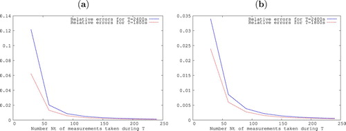$|\overline{\rho }-{\overline{\rho }}_j|/\overline{\rho }$ with respect to the used total number $N_t$ of measurements taken during the considered monitoring time at each of the measuring wells in Table 1. The results obtained using I = 6 are given by:

The behaviour of the relative errors presented in Figure 1 shows that the identified results are improved by increasing the total number $N_t$ of measurements taken in each used measuring well during the monitoring time T. The difference between each two curves in Figure 1 observed for relatively small number $N_t$ of measurements is due to the numerical method used to approximate the integrals with respect to the time defining the cost function. In our experiments, we used the trapezoidal rule whose the approximation error depends on the time step size $\mathrm{\Delta }t=T/N_t$.

Figure 1. (a) Relative errors on $\overline{\psi }$. (b) Relative errors on $\overline{\rho }$.

• Part2: Identification of the storativity function S

As far as the identification of the storativity function is concerned, we apply Option 2. of Global Determination Algorithm developed in Section 4 to identify the function $\overline{S}$ in (57(57) $\overline{S}(x,y)=e^{-{\gamma }_1{L}_{1}x-{\gamma }_2{L}_{2}y-{\gamma }_0}\mathrm{and}\overline{P}(x,y)=\overline{\psi }\overline{S}(x,y)$(57) ) that generated the used measurements i.e. $\overline{S}(x,y)=e^{-{\gamma }_1{L}_{1}x-{\gamma }_2{L}_{2}y-{\gamma }_0}$ in $(0,1{)}^2$. We carried out numerical experiments on identifying $\overline{S}$ for different values of the coefficients ${\gamma }_0,{\gamma }_1$ and ${\gamma }_2$. The obtained results are presented in the following two tables: We give for each experiment $(\mathbf{E})$ the values of ${\gamma }_0,{\gamma }_1$, ${\gamma }_2$ used to generate the measurements, the associated coefficients $B^{i=1,\dots ,I}$ computed from (19(19) $B^i={\displaystyle \frac{{\displaystyle \sum _{n\ge 0}\frac{{\xi }_n(a){\xi }_n(b^i)}{{\mu }_n}{\displaystyle {\int }_0^T\ell (t)(1-e^{-{\mu }_n(T-t)})\mathrm{d}t}}}{{\displaystyle {\int }_0^{T}u(b^i,t)\mathrm{d}t}}}$(19) ) and the identified storativity ${\overline{S}}_{ident}(x,y)=e^{g(x,y)}$.

For each of the two experiments $({\mathbf{E}}_{1,2})$ presented in Table 4, the computed coefficients $B^{i=1,\dots ,I}$ have about the same value. Thus, in view of Option 2. of Global Determination Algorithm, let $N_g=1$ i.e. $g(x,y)=g_0$ in Ω. It follows that setting $g_0=\ln (B^1)$ satisfies with respect to a certain tolerance all equations in (45(45) $g(a)+g(b^i)=2\ln (B^i),\mathrm{for}i=1,\dots ,I$(45) ). Therefore, we set the identified storativity function to ${\overline{S}}_{ident}(x,y)=e^{g_0}=B^1$. Moreover, using the results given in Table 4, we determine $g_0$ for the experiment $({\mathbf{E}}_1)$ from $g_0=\ln (6.67\times {10}^{-3})=-5.01$ and for $({\mathbf{E}}_2)$ from $g_0=\ln (4.41\times {10}^{-5})=-10.03$.

Table 4. Constant storativity: $L_2=100m$, $L_1=\sqrt{\pi }{L}_2$, T = 2400s, I = 6 and $\overline{\psi }=71$.

Measurements with		$B^1$	$B^2$	$B^3$	$B^4$	$B^5$	$B^6$	${\overline{S}}_{ident}(x,y)=e^{g_0}$
$({\mathbf{E}}_1):$	${\gamma }_1=0$	${10}^{-3}\times (6.67$	6.68	$6.67$	6.68	$6.68$	$6.69)$	$g_0=-5.01$
	${\gamma }_2=0$
	${\gamma }_0=5$
$({\mathbf{E}}_2):$	${\gamma }_1=0$	${10}^{-5}\times (4.41$	$4.43$	$4.43$	$4.46$	$4.43$	$4.44)$	$g_0=-10.03$
	${\gamma }_2=0$
	${\gamma }_2=0$

The numerical results obtained for the identification of non-constant storativity are:

Since the coefficients $B^{i=1,\dots ,I}$ associated to each of the two experiments $({\mathbf{E}}_{3,4})$ presented in Table 5 don't have the same value, it follows that a polynomial g with $N_g=1$ cann't satisfy all the equations in (45(45) $g(a)+g(b^i)=2\ln (B^i),\mathrm{for}i=1,\dots ,I$(45) ). However, as the positions of the three measuring wells $b^1,b^2$ and $b^3$ are such that the $3\times 3$ matrix of the linear system (46(46) $\left(\begin{array}{ccc}{a}_1+b_1^1& a_2+b_2^1& 2\\ a_1+b_1^2& a_2+b_2^2& 2\\ a_1+b_1^3& a_2+b_2^3& 2\end{array}\right)\left(\begin{array}{c}{g}_1\\ g_2\\ g_0\end{array}\right)=2\left(\begin{array}{c}\ln (B^1)\\ \ln (B^2)\\ \ln (B^3)\end{array}\right)$(46) ) is invertible, we set $N_g=3$ i.e. $g(x,y)=g_1{L}_{1}x+g_2{L}_{2}y+g_0$. The coefficients $g_0,g_1$ and $g_2$ presented in Table 5 have been determined from solving for each experiment the linear system in (46(46) $\left(\begin{array}{ccc}{a}_1+b_1^1& a_2+b_2^1& 2\\ a_1+b_1^2& a_2+b_2^2& 2\\ a_1+b_1^3& a_2+b_2^3& 2\end{array}\right)\left(\begin{array}{c}{g}_1\\ g_2\\ g_0\end{array}\right)=2\left(\begin{array}{c}\ln (B^1)\\ \ln (B^2)\\ \ln (B^3)\end{array}\right)$(46) ).

Table 5. Varying storativity: $L_2=100m$, $L_1=\sqrt{\pi }{L}_2$, T = 1800s, I = 6 and $\overline{\psi }=71$.

Measurements with		$B^1$	$B^2$	$B^3$	$B^4$	$B^5$	$B^6$	${\overline{S}}_{ident}(x,y)=e^{g(x,y)}$
$({\mathbf{E}}_3):$	${\gamma }_1=0.03$	${10}^{-4}\times (10.17$	8.32	10.72	7.53	11.24	$7.94)$	$g_1=-3.02\times {10}^{-2}$
	${\gamma }_2=0.01$							$g_2=-1.01\times {10}^{-2}$
	${\gamma }_0=5$							$g_0=-4.97$
$({\mathbf{E}}_4):$	${\gamma }_1=0$	${10}^{-4}\times (4.51$	7.44	12.66	4.51	7.44	$2.82)$	$g_1=-2.10\times {10}^{-3}$
	${\gamma }_2=0.05$							$g_2=-5.21\times {10}^{-2}$
	${\gamma }_0=5$							$g_0=-4.74$

6. Conclusion

We developed an identification approach that leads to reconstruct unknown storativity and transmissivity functions occurring in $2D$ groundwater equations. Using an appropriate change of variables, we transformed the groundwater equation into a diffusion-reaction one wherein the diffusion term is the fraction transmissivity/storativity and the reaction coefficient yields the right hand side of a second order nonlinear elliptic partial differential equation satisfied by the unknown storativity function. Under some conditions on the used pumping source as well as on the number and the locations of the employed measuring wells, the developed approach starts by identifying the introduced diffusion and reaction variables. Then, it proposes local and global determination procedures for reconstructing the unknown storativity function. The unknown transmissivity is then deduced from the product of the already determined storativity and fraction transmissivity/storativity functions. The numerical results carried out in this paper show that the developed approach determines accurately the used storativity and fraction functions.

Disclosure statement

No potential conflict of interest was reported by the authors.

References

- Meier PM, Carrera J, Sanchez-Villa X. A numerical study on the relationship between transmissivity and specific capacity in heterogeneous aquifers. Groundwater. 1999;37(4):611–617. doi: 10.1111/j.1745-6584.1999.tb01149.x
- Todd DK. Groundwater hydrology. 2nd ed. New-York: John Wiley; 2004.
- Bulter J. Pumping tests for aquifer evaluation, time for change? Groundwater. 2009;46:615–617.
- Hoeksema RJ, Kitanidis PK. An application of the geostatistical approach to the inverse problem in two-dimensional groundwater modeling. Water Resour Res. 1984;20:1003–1020. doi: 10.1029/WR020i007p01003
- Yeh TJ, Lee C. Time to change the way we collect and analyze data for aquifer characterization. Groundwater. 2007;45:116–118. doi: 10.1111/j.1745-6584.2006.00292.x
- Sterrett RJ. Groundwater and wells. 3rd ed. New Brighton, Minnesota: Johnson Screens; 2007.
- Theis CV. The relation between the lowering of the piezometric surface and the rate and duration of discharge of a well using groundwater storage. Am Geophys Union Trans. 1935;16:519–524. doi: 10.1029/TR016i002p00519
- Cooper HH, Jacob CE. A generalized graphical method for evaluating formation constants and summarizing well-field history. Am Geophys Union Trans. 1946;27(4):526–534. doi: 10.1029/TR027i004p00526
- Jim Yeh TC. Stochastic modelling of groundwater flow and solute transport in aquifers. Hydrlog Process. 1992;6:369–395. doi: 10.1002/hyp.3360060402
- Abdel-Aziz H, Abdel-Gawad A, El-Hadi HA. Parameter estimation of pumping test data using genetic algorithm. In: Thirteenth International Water Technology Conference, IWTC 13; Hurghada-Egypt. 2009.
- Beckie R, Harvey CF. What does a slug test measure: an investigation of instrument response and the effects of heterogeneity. Water Resour Res. 2002;38(12):1–14. doi: 10.1029/2001WR001072
- Castagna M, Bellin A. A Bayesianapproach for inversion of hydraulic tomographic data. Water Resour Res. 2009;45:W04410. doi:10.1029/2008WR007078
- Cleveland TG. Type-curve matching using a computer spreadsheet. Groundwater. 1996;34(3):554–562. doi: 10.1111/j.1745-6584.1996.tb02038.x
- Shapoori V, Peterson TJ, Western AW, et al. Estimating aquifer properties using groundwater hydrograph modelling. Hydrol Process. 2015;29(26):5424–5437. doi:10.1002/hyp.10583
- Nelson RW. In-place measurement of permeability in heterogeneous media: experimental and computational considerations. J Geophys Res. 1960;66:2469–2478. doi: 10.1029/JZ066i008p02469
- Richter GR. An inverse problem for the steady state diffusion equation. SIAM J Math Anal. 1981;41:210–221. doi: 10.1137/0141016
- Rogelio VG, Mauro G, Giansilvio P, et al. The differential system method for the identification of transmissivity and storativity. Transport Porous Media. 1997;26:339–371. doi: 10.1023/A:1006568818150
- Anderson MP, Woessner WW. Applied groundwater modeling. San Diego, CA: Academic Press, Inc.; 1992.
- Bear J. Hydraulics of groundwater. New York: McGraw-Hill; 1979.
- Lions JL. Pointwise control for distributed systems in control and estimation in distributed parameters systems, Edited by Banks H.T. SIAM. 1992.
- Schwartz L. Théorie des distributions. Paris: Hermann; 1966.
- Berestycki H, Hamel F, Nadirashvili N. Elliptic eigenvalue problems with large drift and applications to nonlinear propagation phenomena. Commun Math Phys. 2005;253:451–480. doi: 10.1007/s00220-004-1201-9
- Chen XF, Lou Y. Principal eigenvalue and eigenfunction of an elliptic operator with large advection and its application to a competition model. Indiana Univ Math J. 2008;57:627–658. doi: 10.1512/iumj.2008.57.3204
- El Jai A, Pritchard G. Capteurs et Actionneurs dans l'Analyse des systèmes distribués (RMA 3). Paris: Masson; 1986.
- El Badia A, Ha Duong T. On an inverse source problem for the heat equation: application to a pollution detection problem. J Inverse Ill-Posed Probl. 2002;10:585–599. doi: 10.1515/jiip.2002.10.6.585
- Hamdi A. Detection and identification of multiple unknown time-dependent point sources occurring in 1D evolutionj transport equations. Inverse Probl Sci Eng. 2016;25(4):532–554. doi: 10.1080/17415977.2016.1172224
- Barles G, Blanc A-P, Georgelin C, et al. Remarks on the maximum principle for nonlinear elliptic PDEs with quadratic growth conditions. Ann Scuola Norm Sup Pisa Cl Sci. 1999;28(4):381–404.
- Titchmarsh EC. Introducton to the theory of Fourier integrals. Oxford: Oxford University Press; 1939.
- Alarcon S, Garcia-Mellian J, Quaas A. Keller-Osserman type conditions for some elliptic problems with gradient terms. J Differ Equ. 2012;252(2):886–914. doi: 10.1016/j.jde.2011.09.033