On the Kohn–Vogelius formulation for solving an inverse source problem

Abstract

An inverse source problem related to the Poisson equation is the main concern of this work. Specifically, we deal with the reconstruction of a mass distribution in a geometrical domain from a partial boundary measurement of the associated potential. The considered problem is motivated by various applications such as the identification of geological anomalies underneath the Earth's surface. The proposed approach is based on the Kohn–Vogelius formulation and the topological derivative method. An explicit second-order sensitivity related to circular shaped anomalies is calculated for different examples of the Kohn–Vogelius type functional. Then, the optimal location and size of the unknown support of the mass distribution are characterized as the solution to a minimization problem. The resulting reconstruction procedure is non-iterative and robust with respect to noisy data. Finally, we produce numerical results from four different examples of the Kohn–Vogelius type functional. The results first demonstrate the method and then compare the robustness of each functional in solving the inverse source problem.

Keywords:

• Inverse source problem
• Kohn–Vogelius formulation
• topological derivative method

2010 Mathematics Subject Classifications:

• 49M15
• 31A25
• 35C20
• 35A15

1. Introduction

In this paper, we consider the reconstruction of a mass density distribution with support within a geometrical domain from a boundary measurement of the associated potential. This type of inverse problem has been studied by many authors [1–4]. Isakov [3] proved the identifiability of anomalies with star-shaped or convex in one direction supports. Then, El-Badia and Ha-Duong [1] established the uniqueness in determining multiply-connected ball-shaped anomalies from a single Cauchy data, while Hettlich and Rundell [2] considered a Newton-type iterative method to reconstruct the shape of the anomaly. Liu [4] proposed an iterative approach based on the shape derivative. They applied the gradient descent algorithm (GDA) and trust-region-reflective algorithm (TRA) to detect the location, size, and shape of the source. In the context of gravimetry, Canelas et al. [5] solved this reconstruction problem in the two-dimensional case from complete boundary measurements. They proposed a method which relies on the minimization of a Kohn–Vogelius type functional by using the topological derivative method. In [6], the same authors extend the ideas presented in [5] to cover the two and three spatial dimensions cases with incomplete (partial) boundary measurements.

To reconstruct the location, size, shape and number of the mass density distributions in the geometrical domain, we follow the ideas presented in [6]. The proposed approach is based on the Kohn–Vogelius formulation [7] and the topological derivative method [8]. More precisely, we reconstruct the support ${\omega }^{\ast }\subset \mathrm{\Omega }$ of a source-term, where $\mathrm{\Omega }\subset {\mathbb{R}}^2$, with boundary $\mathrm{\partial }\mathrm{\Omega }$, from a partial boundary measurement of the associated potential on the boundary ${\mathrm{\Gamma }}_M\subset \mathrm{\partial }\mathrm{\Omega }$, but without using the Newtonian potential to complement the unavailable information about the hidden boundary as presented in [6].

The Kohn–Vogelius shape functional measures the misfit between the solutions of two auxiliary problems containing information about the boundary measurements. It is a self regularization technique that rephrases the inverse problem as an optimization problem where the support of the anomalies is the unknown variable. The minimum of the Kohn–Vogelius objective functional is reached when the unknown support coincides with the actual one. The topology optimization problem consists of minimizing the variation of the Kohn–Vogelius type functional with respect to a class of mass distributions defined by a finite number of ball-shaped trial anomalies.

An asymptotic expansion of the Kohn–Vogelius functional with respect to the circular perturbations is computed using the topological derivative method. The second-order topological gradient is applied in the context of the proposed source reconstruction problem. In particular, four different versions of the Kohn–Vogelius shape functional are considered: the $L^2({\mathrm{\Gamma }}_M)$-norm, $L^2(\mathrm{\Omega })$-norm, $H^1(\mathrm{\Omega })$-seminorm and $H^1(\mathrm{\Omega })$-norm of the error function. The main idea of this type of functional was first introduced by Wexler et al. [9] where a procedure to detect the unknown impedance from boundary measurements was proposed. Then, Kohn and Vogelius [7] suggested a modification of Wexler's procedure to make it an alternating direction one by proposing a new misfit gap-cost functional. Since then, this formulation has been used to solve various inverse problems [6,10,11]. Variants of this type of inverse problem have applications in various fields such as gravimetry, where the goal is to determine the Earth's density distribution from measurements of the gravity and its derivatives on the surface of the Earth [3].

By uniqueness of the auxiliary forward problems, all objective functions are equivalent in theory. From the practical point of view, however, their effectiveness may depend on the modelling uncertainties (noisy data) and discretization strategies. The main concern of this paper is to compare the four metrics in different scenarios, which represents the main originality of the current article in comparison to Canelas et al. [6]. The findings reported here are useful not only for readers interested in the topological derivative method but also for anyone dealing with the inverse source problem and related reconstruction problems.

The paper is organized as follows. In Section 2 the inverse problem to be considered is rewritten in the form of a topology optimization problem, which consists of minimizing a Kohn–Vogelius shape functional with respect to a set of ball-shaped anomalies. To solve this inverse problem the concept of second-order topological derivative is introduced in Section 3. The resulting Newton-type method is presented in Section 4, together with the associated reconstruction algorithm. In Section 5, we present numerical examples that demonstrate the effectiveness of the devised reconstruction algorithm and compare the distance functions proposed. Finally, in Section 6 there are concluding remarks.

2. Inverse source problem

Consider determining a source term $f^{\ast }$ for the following elliptic problem: (1) $\{\begin{array}{ll}-\mathrm{\Delta }u=f^{\ast }& \mathrm{in}\mathrm{\Omega },\\ {\mathrm{\partial }}_{\nu }u=0& \mathrm{on}{\mathrm{\Gamma }}_M,\\ u=0& \mathrm{on}{\mathrm{\Gamma }}_0:=\mathrm{\partial }\mathrm{\Omega }\mathrm{\setminus }\overline{{\mathrm{\Gamma }}_M},\end{array}$(1) from the given boundary data: $u=u^{\ast }\text{on}{\mathrm{\Gamma }}_M,$ where $\mathrm{\Omega }\subset {\mathbb{R}}^2$ is an open and bounded domain with a Lipschitz boundary $\mathrm{\partial }\mathrm{\Omega }$, and ${\mathrm{\Gamma }}_M$ is an open subset of $\mathrm{\partial }\mathrm{\Omega }$ with a non-void interior (with respect to the boundary topology). In addition, ${\mathrm{\partial }}_{\nu }u=\mathrm{\nabla }u\cdot \nu$ and ν is the unit outward normal vector to $\mathrm{\partial }\mathrm{\Omega }$.

The major difficulty with this inverse problem is that the general source terms are unidentifiable due to the nature of the boundary data. To handle this question of uniqueness, a priori assumptions on the class of sources to be detected are made. Hence, the source term $f^{\ast }$ is modelled as a discontinuous source, namely, $f^{\ast }={\chi }_{{\omega }^{\ast }}$ where ${\chi }_{{\omega }^{\ast }}$ is the characteristic function of the unknown sub-domain ${\omega }^{\ast }\subset \mathrm{\Omega }$, that have to be recovered from partial boundary measurement of the associated potential on ${\mathrm{\Gamma }}_M$.

The inverse problem to be solved consists in finding ${\chi }_{{\omega }^{\ast }}\in \mathcal{A}(\mathrm{\Omega })$ such that the boundary value problem (1(1) $\{\begin{array}{ll}-\mathrm{\Delta }u=f^{\ast }& \mathrm{in}\mathrm{\Omega },\\ {\mathrm{\partial }}_{\nu }u=0& \mathrm{on}{\mathrm{\Gamma }}_M,\\ u=0& \mathrm{on}{\mathrm{\Gamma }}_0:=\mathrm{\partial }\mathrm{\Omega }\mathrm{\setminus }\overline{{\mathrm{\Gamma }}_M},\end{array}$(1) ) is satisfied. The set of admissible solutions $\mathcal{A}(\mathrm{\Omega })$ is given by characteristic functions of the form: (2) $\mathcal{A}(\mathrm{\Omega })=\{{\chi }_{\omega }:\mathrm{\Omega }\mapsto \mathbb{R}|{\chi }_{\omega }=1\mathrm{in}\omega \mathrm{and}{\chi }_{\omega }=0\mathrm{in}\mathrm{\Omega }\setminus \omega \},$(2) where $\omega \subset \mathrm{\Omega }$ is a Lebesgue measurable set. However, the difficulty is that the inverse problem (1(1) $\{\begin{array}{ll}-\mathrm{\Delta }u=f^{\ast }& \mathrm{in}\mathrm{\Omega },\\ {\mathrm{\partial }}_{\nu }u=0& \mathrm{on}{\mathrm{\Gamma }}_M,\\ u=0& \mathrm{on}{\mathrm{\Gamma }}_0:=\mathrm{\partial }\mathrm{\Omega }\mathrm{\setminus }\overline{{\mathrm{\Gamma }}_M},\end{array}$(1) ) is an over-determined boundary value problem and there is a lack of stability in the sense of Hadamard. In order to deal with the over-determined problem, (1(1) $\{\begin{array}{ll}-\mathrm{\Delta }u=f^{\ast }& \mathrm{in}\mathrm{\Omega },\\ {\mathrm{\partial }}_{\nu }u=0& \mathrm{on}{\mathrm{\Gamma }}_M,\\ u=0& \mathrm{on}{\mathrm{\Gamma }}_0:=\mathrm{\partial }\mathrm{\Omega }\mathrm{\setminus }\overline{{\mathrm{\Gamma }}_M},\end{array}$(1) ) is separated into two well posed problems: given ${\chi }_{\omega }\in \mathcal{A}(\mathrm{\Omega })$, find $u^D$ and $u^N$ such that (3) $\{\begin{array}{ll}-\mathrm{\Delta }{u}^D={\chi }_{\omega }& \mathrm{in}\mathrm{\Omega }\\ u^D=u^{\ast }& \mathrm{on}{\mathrm{\Gamma }}_M\\ u^D=0& \mathrm{on}{\mathrm{\Gamma }}_0\end{array}\mathrm{and}\{\begin{array}{ll}-\mathrm{\Delta }{u}^N={\chi }_{\omega }& \mathrm{in}\mathrm{\Omega }\\ {\mathrm{\partial }}_{\nu }{u}^N=0& \mathrm{on}{\mathrm{\Gamma }}_M\\ u^N=0\mathrm{on}& {\mathrm{\Gamma }}_0\end{array}.$(3) These problems assume that the medium is big enough that the potential decays to zero on the portion of the boundary that is not measured (${\mathrm{\Gamma }}_0=\mathrm{\partial }\mathrm{\Omega }\setminus {\mathrm{\Gamma }}_M$). The solution to (1(1) $\{\begin{array}{ll}-\mathrm{\Delta }u=f^{\ast }& \mathrm{in}\mathrm{\Omega },\\ {\mathrm{\partial }}_{\nu }u=0& \mathrm{on}{\mathrm{\Gamma }}_M,\\ u=0& \mathrm{on}{\mathrm{\Gamma }}_0:=\mathrm{\partial }\mathrm{\Omega }\mathrm{\setminus }\overline{{\mathrm{\Gamma }}_M},\end{array}$(1) ), due to the uniqueness of the traces of $u^D$ and $u^N$ on ${\mathrm{\Gamma }}_M$, is: (4) $\mathrm{If}{\chi }_{\omega }={\chi }_{{\omega }^{\ast }}\Rightarrow u^D=u^N.$(4) Then, we find the solution by formulating the inverse problem as a topology optimization problem which minimizes the difference between $u^D$ and $u^N$: (5) $\underset{{\chi }_w\in \mathcal{A}(\mathrm{\Omega })}{\mathrm{Minimize}}\rho (u^D-u^N)$(5) where $\rho (u^D-u^N)$ represents the distance between $u^D$ and $u^N$ in some appropriated norm. To measure this distance we will consider different examples of the Kohn–Vogelius type functional, such as the $L^2({\mathrm{\Gamma }}_M)$-norm, $L^2(\mathrm{\Omega })$-norm, $H^1(\mathrm{\Omega })$-seminorm, and $H^1(\mathrm{\Omega })$-norm. Note that in this context, ω can be interpreted as an initial guess for the true anomaly ${\omega }^{\ast }$. Since ω is arbitrary, we will assume later trivial initial guess given by $\omega =\varnothing$.

Since the inverse source problem (1(1) $\{\begin{array}{ll}-\mathrm{\Delta }u=f^{\ast }& \mathrm{in}\mathrm{\Omega },\\ {\mathrm{\partial }}_{\nu }u=0& \mathrm{on}{\mathrm{\Gamma }}_M,\\ u=0& \mathrm{on}{\mathrm{\Gamma }}_0:=\mathrm{\partial }\mathrm{\Omega }\mathrm{\setminus }\overline{{\mathrm{\Gamma }}_M},\end{array}$(1) ) is rewritten as a topology optimization problem (5(5) $\underset{{\chi }_w\in \mathcal{A}(\mathrm{\Omega })}{\mathrm{Minimize}}\rho (u^D-u^N)$(5) ), we seek to solve the optimization problem by using the topological derivative method which is described in the next section.

3. Topological sensitivity analysis

The topological derivative measures the sensitivity of a given shape function with respect to infinitesimal geometry perturbations such as the creation of inclusions, cracks, cavities, inhomogeneities, or source-terms. Theoretically, the topological sensitivity concept is the first term of the asymptotic expansion of such shape functions with respect to the small parameter that measures the size of the introduced perturbation. This idea was first developed by Schumacher [12] under the name of bubble method in the context of compliance minimization in linear elasticity, followed by Sokołowski and Żochowski [13] and Céa et al. [14]. Since then, this concept has been successfully applied to many relevant scientific and engineering problems such as inverse problems [15–20], topology optimization [21–24], image processing [25–28], damage [29,30] and fracture [31,32] evolution modelling, and many other applications.

To present the basic idea of this method, we consider an open and bounded domain $\mathrm{\Omega }\subset {\mathbb{R}}^d$ $(d\in \{2,3\})$ and a non-smooth perturbation confined in a small set ${\omega }_{\epsilon ,z}$ of size $\epsilon >0$ centred at an arbitrary point z of Ω such that ${\omega }_{\epsilon ,z}⋐\mathrm{\Omega }$. To be more precise, in this context ${\omega }_{\epsilon ,z}$ represents the topological perturbed counterpart of the initial guess ω. We introduce a characteristic function $x\mapsto \chi (x),x\in \mathrm{\Omega }$, associated with the unperturbed domain, namely $\chi ={\mathbb{1}}_{\mathrm{\Omega }}$. Similarly, we define a characteristic function $x\mapsto {\chi }_{\epsilon }(z,x),x\in \mathrm{\Omega }$, associated to the topologically perturbed domain. In the case of a perforation, for instance, ${\chi }_{\epsilon }(z)={\mathbb{1}}_{\mathrm{\Omega }}-{\mathbb{1}}_{{\omega }_{\epsilon ,z}}$ and the perturbed domain is given by ${\mathrm{\Omega }}_{\epsilon ,z}=\mathrm{\Omega }\mathrm{\setminus }\overline{{\omega }_{\epsilon ,z}}$. Then, for a given shape functional $\mathcal{G}({\chi }_{\epsilon }(z))$ associated with the topologically perturbed domain, the topological sensitivity analysis method would provide an asymptotic expansion of $\mathcal{G}({\chi }_{\epsilon }(z))$ of the form: (6) $\mathcal{G}({\chi }_{\epsilon }(z))=\mathcal{G}(\chi )+f_1(\epsilon )\mathcal{T}(z)+o(f_1(\epsilon )),$(6) where:

• $\mathcal{G}(\chi )$ is the shape functional associated with the unperturbed domain;

• $\epsilon \mapsto f_1(\epsilon )$ is a scalar positive function such that $f_1(\epsilon )\to 0$ when $\epsilon \to 0$;

• the function $z\mapsto \mathcal{T}(z)$ is called the first-order ‘topological derivative’ or ‘topological sensitivity’ of the shape functional $\mathcal{G}$ at z and plays the role of leading term of the variation $\mathcal{G}({\chi }_{\epsilon }(z))-\mathcal{G}(\chi )$. Mathematically, we express it as: $\mathcal{T}(z):=\underset{\epsilon \to 0}{lim}\frac{\mathcal{G}({\chi }_{\epsilon }(z))-\mathcal{G}(\chi )}{f_1(\epsilon )}.$

We can define the second-order topological derivative of the shape functional $\mathcal{G}$ at z by expanding the remainder term $o(f_1(\epsilon ))$ in (6(6) $\mathcal{G}({\chi }_{\epsilon }(z))=\mathcal{G}(\chi )+f_1(\epsilon )\mathcal{T}(z)+o(f_1(\epsilon )),$(6) ). Therefore, an asymptotic expansion of the functional $\mathcal{G}$ at z can be in the following form: (7) $\mathcal{G}({\chi }_{\epsilon }(z))=\mathcal{G}(\chi )+f_1(\epsilon )\mathcal{T}(z)+f_2(\epsilon ){\mathcal{T}}^2(z)+o(f_2(\epsilon )),$(7) where:

• $\epsilon \mapsto f_2(\epsilon )$ is a scalar positive function such that $f_2(\epsilon )=o(f_1(\epsilon ))$ and $f_2(\epsilon )\to 0$ when $\epsilon \to 0$;

• ${\mathcal{T}}^2(z)$ denotes the second-order topological derivative of the shape function $\mathcal{G}$ at z, which can be defined as ${\mathcal{T}}^2(z):=\underset{\epsilon \to 0}{lim}\frac{\mathcal{G}({\chi }_{\epsilon }(z))-\mathcal{G}(\chi )-f_1(\epsilon )\mathcal{T}(z)}{f_2(\epsilon )}.$

In this paper, the problem is perturbed by introducing balls in order to determine the sensitivities. Consider n ball-shaped anomalies, with radii and centres $\epsilon =({\epsilon }_1,\dots ,{\epsilon }_n)$ and $\xi =(z_1,\dots ,z_n)$ respectively. This results in the characteristic function: (8) ${\chi }_{{\omega }_{\epsilon }}={\chi }_{\omega }+\sum _{i=1}^n{\chi }_{{\mathcal{B}}_{{\epsilon }_i}(z_i)}$(8) where ${\mathcal{B}}_{{\epsilon }_i}(z_i)$ denotes a ball of radius ${\epsilon }_i$ and centre $z_i$ in Ω, for $i=1,\dots ,n$. We assume that ${\mathcal{B}}_{{\epsilon }_i}(z_i)⋐\mathrm{\Omega }$ such that ${\mathcal{B}}_{{\epsilon }_i}(z_i)\cap {\mathcal{B}}_{{\epsilon }_j}(z_j)=\mathrm{\varnothing }$ for $i\ne j$. Therefore, given ${\chi }_{{\omega }_{\epsilon }}\in \mathcal{A}(\mathrm{\Omega })$, the perturbed counterparts of problems (3(3) $\{\begin{array}{ll}-\mathrm{\Delta }{u}^D={\chi }_{\omega }& \mathrm{in}\mathrm{\Omega }\\ u^D=u^{\ast }& \mathrm{on}{\mathrm{\Gamma }}_M\\ u^D=0& \mathrm{on}{\mathrm{\Gamma }}_0\end{array}\mathrm{and}\{\begin{array}{ll}-\mathrm{\Delta }{u}^N={\chi }_{\omega }& \mathrm{in}\mathrm{\Omega }\\ {\mathrm{\partial }}_{\nu }{u}^N=0& \mathrm{on}{\mathrm{\Gamma }}_M\\ u^N=0\mathrm{on}& {\mathrm{\Gamma }}_0\end{array}.$(3) ) are: find $u_{\epsilon }^D$ and $u_{\epsilon }^N$ such that (9) $\{\begin{array}{ll}-\mathrm{\Delta }{u}_{\epsilon }^D={\chi }_{{\omega }_{\epsilon }}& \mathrm{in}\mathrm{\Omega }\\ u_{\epsilon }^D=u^{\ast }& \mathrm{on}{\mathrm{\Gamma }}_M\\ u_{\epsilon }^D=0& \mathrm{on}{\mathrm{\Gamma }}_0\end{array}\mathrm{and}\{\begin{array}{ll}-\mathrm{\Delta }{u}_{\epsilon }^N={\chi }_{{\omega }_{\epsilon }}& \mathrm{in}\mathrm{\Omega }\\ {\mathrm{\partial }}_{\nu }{u}_{\epsilon }^N=0& \mathrm{on}{\mathrm{\Gamma }}_M\\ u_{\epsilon }^N=0& \mathrm{on}{\mathrm{\Gamma }}_0\end{array}$(9)

3.1. Asymptotic analysis of the solution

Let us introduce the following ansätze for the solutions to the perturbed problems (9(9) $\{\begin{array}{ll}-\mathrm{\Delta }{u}_{\epsilon }^D={\chi }_{{\omega }_{\epsilon }}& \mathrm{in}\mathrm{\Omega }\\ u_{\epsilon }^D=u^{\ast }& \mathrm{on}{\mathrm{\Gamma }}_M\\ u_{\epsilon }^D=0& \mathrm{on}{\mathrm{\Gamma }}_0\end{array}\mathrm{and}\{\begin{array}{ll}-\mathrm{\Delta }{u}_{\epsilon }^N={\chi }_{{\omega }_{\epsilon }}& \mathrm{in}\mathrm{\Omega }\\ {\mathrm{\partial }}_{\nu }{u}_{\epsilon }^N=0& \mathrm{on}{\mathrm{\Gamma }}_M\\ u_{\epsilon }^N=0& \mathrm{on}{\mathrm{\Gamma }}_0\end{array}$(9) ): (10) $\begin{array}{rl}{u}_{\epsilon }^D(x)& =u^D(x)+\sum _{i=1}^n\pi {\epsilon }_i^2{v}_{{\epsilon }_i}^D(x)\end{array}$(10) (11) $\begin{array}{rl}{u}_{\epsilon }^N(x)& =u^N(x)+\sum _{i=1}^n\pi {\epsilon }_i^2{v}_{{\epsilon }_i}^N(x)\end{array}$(11) where $v_{{\epsilon }_i}^D$ and $v_{{\epsilon }_i}^N$ are the solutions of the following auxiliary boundary value problems for $i=1,\dots ,n$: find $v_{{\epsilon }_i}^D$ and $v_{{\epsilon }_i}^N$ such that (12) $\{\begin{array}{ll}-\mathrm{\Delta }{v}_{{\epsilon }_i}^D={\displaystyle \frac{1}{\pi {\epsilon }_i^2}}{\chi }_{{\mathcal{B}}_{{\epsilon }_i}(z_i)}& \mathrm{in}\mathrm{\Omega }\\ v_{{\epsilon }_i}^D=0& \mathrm{on}{\mathrm{\Gamma }}_M\\ v_{{\epsilon }_i}^D=0& \mathrm{on}{\mathrm{\Gamma }}_0\end{array}\mathrm{and}\{\begin{array}{ll}-\mathrm{\Delta }{v}_{{\epsilon }_i}^N={\displaystyle \frac{1}{\pi {\epsilon }_i^2}}{\chi }_{{\mathcal{B}}_{{\epsilon }_i}(z_i)}& \mathrm{in}\mathrm{\Omega }\\ {\mathrm{\partial }}_{\nu }{v}_{{\epsilon }_i}^N=0& \mathrm{on}{\mathrm{\Gamma }}_M\\ v_{{\epsilon }_i}^N=0& \mathrm{on}{\mathrm{\Gamma }}_0\end{array}$(12) Since $v_{{\epsilon }_i}^D$ and $v_{{\epsilon }_i}^N$ depend on ${\epsilon }_i$ in the ball ${\mathcal{B}}_{{\epsilon }_i}(z_i)$, separate them into two parts: (13) $\begin{array}{rl}{v}_{{\epsilon }_i}^D(x)& =p_{{\epsilon }_i}(x)+q_i^D(x)\end{array}$(13) (14) $\begin{array}{rl}{v}_{{\epsilon }_i}^N(x)& =p_{{\epsilon }_i}(x)+q_i^N(x)\end{array}$(14) where $p_{{\epsilon }_i}$ is solution of the following boundary value problem defined in a big ball ${\mathcal{B}}_R(z_i)\supset \mathrm{\Omega }$ of radius R and centre at $z_i$: find $p_{{\epsilon }_i}$ such that (15) $\{\begin{array}{ll}-\mathrm{\Delta }{p}_{{\epsilon }_i}={\displaystyle \frac{1}{\pi {\epsilon }_i^2}}{\chi }_{{\mathcal{B}}_{{\epsilon }_i}(z_i)}& \mathrm{in}{\mathcal{B}}_R(z_i)\\ p_{{\epsilon }_i}={\displaystyle \frac{1}{2\pi }}\ln R& \mathrm{on}\mathrm{\partial }{\mathcal{B}}_R(z_i)\end{array}$(15) The above boundary value problem admits the explicit solution, namely: (16) $p_{{\epsilon }_i}(x)=\{\begin{array}{ll}-{\displaystyle \frac{1}{4\pi }}({\displaystyle \frac{\Vert x-z_i{\Vert }^2}{{\epsilon }_i^2}}+2\ln {\epsilon }_i-1)& x\in {\mathcal{B}}_{{\epsilon }_i}(z_i)\\ -{\displaystyle \frac{1}{2\pi }}\ln \Vert x-z_i\Vert & x\in {\mathcal{B}}_R(z_i)\setminus {\mathcal{B}}_{{\epsilon }_i}(z_i)\end{array}$(16) Finally, $q_i^D$ and $q_i^N$ must compensate for the discrepancies left by $p_{{\epsilon }_i}$ on $\mathrm{\partial }\mathrm{\Omega }$. In particular, they are the solutions to the following boundary value problems: find $q_i^D$ and $q_i^N$ such that (17) $\begin{array}{rl}& \{\begin{array}{ll}-\mathrm{\Delta }{q}_i^D=0& \mathrm{in}\mathrm{\Omega }\\ q_i^D={\displaystyle \frac{1}{2\pi }}\ln \Vert x-z_i\Vert & \mathrm{on}\mathrm{\partial }\mathrm{\Omega }\end{array}\end{array}$(17) (18) $\begin{array}{rl}& \{\begin{array}{ll}-\mathrm{\Delta }{q}_i^N=0& \mathrm{in}\mathrm{\Omega }\\ {\mathrm{\partial }}_{\nu }{q}_i^N={\displaystyle \frac{1}{2\pi }}{\displaystyle \frac{x-z_i}{\Vert x-z_i{\Vert }^2}}\cdot \nu & \mathrm{on}{\mathrm{\Gamma }}_M\\ q_i^N={\displaystyle \frac{1}{2\pi }}\ln \Vert x-z_i\Vert & \mathrm{on}{\mathrm{\Gamma }}_0\end{array}\end{array}$(18) Therefore, the difference between $u_{\epsilon }^D$ and $u_{\epsilon }^N$ is simply given by (19) $u_{\epsilon }^D-u_{\epsilon }^N=u^D-u^N+\sum _{i=1}^n\pi {\epsilon }_i^2{h}_i,$(19) with $h_i=q_i^D-q_i^N$. The following result justifies the ansätze (10(10) $\begin{array}{rl}{u}_{\epsilon }^D(x)& =u^D(x)+\sum _{i=1}^n\pi {\epsilon }_i^2{v}_{{\epsilon }_i}^D(x)\end{array}$(10) ) and (11(11) $\begin{array}{rl}{u}_{\epsilon }^N(x)& =u^N(x)+\sum _{i=1}^n\pi {\epsilon }_i^2{v}_{{\epsilon }_i}^N(x)\end{array}$(11) ):

Lemma 3.1

Let us consider the expansion (19(19) $u_{\epsilon }^D-u_{\epsilon }^N=u^D-u^N+\sum _{i=1}^n\pi {\epsilon }_i^2{h}_i,$(19) ), then the following estimate holds true (20) $\Vert w_{\epsilon }-w{\Vert }_{H^1(\mathrm{\Omega })}\le C|\epsilon {|}^2,$(20) where $w_{\epsilon }:=u_{\epsilon }^D-u_{\epsilon }^N,$ $w:=u^D-u^N,$ $|\epsilon |={\epsilon }_1+\cdots +{\epsilon }_n$ and C is a constant independent of the small parameters ${\epsilon }_i,$ for $i=1,\dots ,n$.

Proof.

By taking into account the triangular inequality in expansion (19(19) $u_{\epsilon }^D-u_{\epsilon }^N=u^D-u^N+\sum _{i=1}^n\pi {\epsilon }_i^2{h}_i,$(19) ), we have (21) $\Vert (u_{\epsilon }^D-u_{\epsilon }^N)-(u^D-u^N){\Vert }_{H^1(\mathrm{\Omega })}\le C_1\sum _{i=1}^n{\epsilon }_i^2\Vert h_i{\Vert }_{H^1(\mathrm{\Omega })},$(21) which leads to the result provided that each $h_i$ is independent of ${\epsilon }_i$, for $i=1,\dots ,n$.

3.2. Asymptotic analysis of the distance function

In this section, we want to find a better approximation ${\omega }_{\epsilon }$ than the initial guess ω to the target ${\omega }^{\ast }$. Therefore, let us propose an expansion of the form: (22) ${\mathrm{\Psi }}_n(\alpha ,\xi )=\alpha \cdot d(\xi )+\frac{1}{2}H(\xi )\alpha \cdot \alpha ,$(22) where ${\mathrm{\Psi }}_n(\alpha ,\xi )=\rho (u_{\epsilon }^D-u_{\epsilon }^N)-\rho (u^D-u^N)$ and vector $\alpha =({\alpha }_1,\dots {\alpha }_n)$, with ${\alpha }_i=\pi {\epsilon }_i^2$, remembering that n is the number of anomalies to be reconstructed, ξ are their locations and α their sizes (areas). Note that the number of anomalies n to be reconstructed is arbitrary. However, since we are interested in comparing different distance functions, for the sake of simplicity we assume that n is given. Finally, vector d and matrix H, with entries (23) $d(\xi )=\left(\begin{array}{c}{d}_1\\ d_2\\ ⋮\\ d_n\end{array}\right)\mathrm{and}H(\xi )=\left(\begin{array}{cccc}{H}_{11}& H_{12}& \cdots & H_{1n}\\ H_{21}& H_{22}& \cdots & H_{2n}\\ ⋮& ⋮& \ddots & ⋮\\ H_{n1}& H_{n2}& \cdots & H_{nn}\end{array}\right),$(23) will be defined according to each distance function.

3.2.1. $L^2({\mathrm{\Gamma }}_M)$-norm

Consider $\rho (u^D-u^N)={\mathcal{J}}_1(u^D,u^N)$, with (24) ${\mathcal{J}}_1(u^D,u^N):={\int }_{{\mathrm{\Gamma }}_M}|u^D-u^N{|}^2.$(24) The associated topological asymptotic expansion is: (25) $\begin{array}{rl}{\mathcal{J}}_1(u_{\epsilon }^D,u_{\epsilon }^N)& ={\int }_{{\mathrm{\Gamma }}_M}|u_{\epsilon }^D-u_{\epsilon }^N{|}^2\\ & ={\mathcal{J}}_1(u^D,u^N)+2\sum _{i=1}^n\pi {\epsilon }_i^2{\int }_{{\mathrm{\Gamma }}_M}(u^D-u^N)h_i+\sum _{i,j=1}^n\pi {\epsilon }_i^2\pi {\epsilon }_j^2{\int }_{{\mathrm{\Gamma }}_M}{h}_i{h}_j\end{array}$(25) such that the entries of the vector d and matrix H are: (26) $d_i=2{\int }_{{\mathrm{\Gamma }}_M}(u^D-u^N)h_i\mathrm{and}{H}_{ij}=2{\int }_{{\mathrm{\Gamma }}_M}{h}_i{h}_j$(26)

3.2.2. $L^2(\mathrm{\Omega })$-norm

Consider $\rho (u^D-u^N)={\mathcal{J}}_2(u^D,u^N)$, with (27) ${\mathcal{J}}_2(u^D,u^N):={\int }_{\mathrm{\Omega }}|u^D-u^N{|}^2.$(27) The associated topological asymptotic expansion is: (28) $\begin{array}{rl}{\mathcal{J}}_2(u_{\epsilon }^D,u_{\epsilon }^N)& ={\int }_{\mathrm{\Omega }}|u_{\epsilon }^D-u_{\epsilon }^N{|}^2\\ & ={\mathcal{J}}_2(u^D,u^N)+2\sum _{i=1}^n\pi {\epsilon }_i^2{\int }_{\mathrm{\Omega }}(u^D-u^N)h_i+\sum _{i,j=1}^n\pi {\epsilon }_i^2\pi {\epsilon }_j^2{\int }_{\mathrm{\Omega }}{h}_i{h}_j\end{array}$(28) such that the entries of the vector d and matrix H are: (29) $d_i=2{\int }_{\mathrm{\Omega }}(u^D-u^N)h_i\mathrm{and}{H}_{ij}=2{\int }_{\mathrm{\Omega }}{h}_i{h}_j$(29)

3.2.3. $H^1(\mathrm{\Omega })$-seminorm

Consider $\rho (u^D-u^N)={\mathcal{J}}_3(u^D,u^N)$, with (30) ${\mathcal{J}}_3(u^D,u^N):={\int }_{\mathrm{\Omega }}\Vert \mathrm{\nabla }(u^D-u^N){\Vert }^2.$(30) Its associated topological asymptotic expansion is: (31) $\begin{array}{rl}{\mathcal{J}}_3(u_{\epsilon }^D,u_{\epsilon }^N)& ={\int }_{\mathrm{\Omega }}\Vert \mathrm{\nabla }(u_{\epsilon }^D-u_{\epsilon }^N){\Vert }^2\\ & ={\mathcal{J}}_3(u^D,u^N)+2\sum _{i=1}^n\pi {\epsilon }_i^2{\int }_{\mathrm{\Omega }}\mathrm{\nabla }(u^D-u^N)\cdot \mathrm{\nabla }{h}_i\\ & +\sum _{i,j=1}^n\pi {\epsilon }_i^2\pi {\epsilon }_j^2{\int }_{\mathrm{\Omega }}\mathrm{\nabla }{h}_i\cdot \mathrm{\nabla }{h}_j\end{array}$(31) such that the entries of the vector d and matrix H are: (32) $d_i=2{\int }_{\mathrm{\Omega }}\mathrm{\nabla }(u^D-u^N)\cdot \mathrm{\nabla }{h}_i\mathrm{and}{H}_{ij}=2{\int }_{\mathrm{\Omega }}\mathrm{\nabla }{h}_i\cdot \mathrm{\nabla }{h}_j$(32)

3.2.4. $H^1(\mathrm{\Omega })$-norm

Consider $\rho (u^D-u^N)={\mathcal{J}}_2(u^D,u^N)+{\mathcal{J}}_3(u^D,u^N)$, with (33) ${\mathcal{J}}_2(u^D,u^N)+{\mathcal{J}}_3(u^D,u^N)={\int }_{\mathrm{\Omega }}|u^D-u^N{|}^2+{\int }_{\mathrm{\Omega }}\Vert \mathrm{\nabla }(u^D-u^N){\Vert }^2.$(33) Its associated topological asymptotic expansion is: (34) $\begin{array}{rl}& {\mathcal{J}}_2(u_{\epsilon }^D,u_{\epsilon }^N)+{\mathcal{J}}_3(u_{\epsilon }^D,u_{\epsilon }^N)\\ & ={\mathcal{J}}_2(u^D,u^N)+{\mathcal{J}}_3(u^D,u^N)+2\sum _{i=1}^n\pi {\epsilon }_i^2{\int }_{\mathrm{\Omega }}(u^D-u^N)h_i+\sum _{i,j=1}^n\pi {\epsilon }_i^2\pi {\epsilon }_j^2{\int }_{\mathrm{\Omega }}{h}_i{h}_j\\ & +2\sum _{i=1}^n\pi {\epsilon }_i^2{\int }_{\mathrm{\Omega }}\mathrm{\nabla }(u^D-u^N)\cdot \mathrm{\nabla }{h}_i+\sum _{i,j=1}^n\pi {\epsilon }_i^2\pi {\epsilon }_j^2{\int }_{\mathrm{\Omega }}\mathrm{\nabla }{h}_i\cdot \mathrm{\nabla }{h}_j\end{array}$(34) such that the entries of the vector d and matrix H are: (35) $\begin{array}{rl}{d}_i& =2{\int }_{\mathrm{\Omega }}((u^D-u^N)h_i+\mathrm{\nabla }(u^D-u^N)\cdot \mathrm{\nabla }{h}_i)\end{array}$(35) (36) $\begin{array}{rl}{H}_{ij}& =2{\int }_{\mathrm{\Omega }}(h_i{h}_j+\mathrm{\nabla }{h}_i\cdot \mathrm{\nabla }{h}_j)\end{array}$(36)

Remark 3.2

Since we are dealing with topological perturbation given by circular anomalies, the resulting expansions (25(25) $\begin{array}{rl}{\mathcal{J}}_1(u_{\epsilon }^D,u_{\epsilon }^N)& ={\int }_{{\mathrm{\Gamma }}_M}|u_{\epsilon }^D-u_{\epsilon }^N{|}^2\\ & ={\mathcal{J}}_1(u^D,u^N)+2\sum _{i=1}^n\pi {\epsilon }_i^2{\int }_{{\mathrm{\Gamma }}_M}(u^D-u^N)h_i+\sum _{i,j=1}^n\pi {\epsilon }_i^2\pi {\epsilon }_j^2{\int }_{{\mathrm{\Gamma }}_M}{h}_i{h}_j\end{array}$(25) ), (28(28) $\begin{array}{rl}{\mathcal{J}}_2(u_{\epsilon }^D,u_{\epsilon }^N)& ={\int }_{\mathrm{\Omega }}|u_{\epsilon }^D-u_{\epsilon }^N{|}^2\\ & ={\mathcal{J}}_2(u^D,u^N)+2\sum _{i=1}^n\pi {\epsilon }_i^2{\int }_{\mathrm{\Omega }}(u^D-u^N)h_i+\sum _{i,j=1}^n\pi {\epsilon }_i^2\pi {\epsilon }_j^2{\int }_{\mathrm{\Omega }}{h}_i{h}_j\end{array}$(28) ), (31(31) $\begin{array}{rl}{\mathcal{J}}_3(u_{\epsilon }^D,u_{\epsilon }^N)& ={\int }_{\mathrm{\Omega }}\Vert \mathrm{\nabla }(u_{\epsilon }^D-u_{\epsilon }^N){\Vert }^2\\ & ={\mathcal{J}}_3(u^D,u^N)+2\sum _{i=1}^n\pi {\epsilon }_i^2{\int }_{\mathrm{\Omega }}\mathrm{\nabla }(u^D-u^N)\cdot \mathrm{\nabla }{h}_i\\ & +\sum _{i,j=1}^n\pi {\epsilon }_i^2\pi {\epsilon }_j^2{\int }_{\mathrm{\Omega }}\mathrm{\nabla }{h}_i\cdot \mathrm{\nabla }{h}_j\end{array}$(31) ) and (34(34) $\begin{array}{rl}& {\mathcal{J}}_2(u_{\epsilon }^D,u_{\epsilon }^N)+{\mathcal{J}}_3(u_{\epsilon }^D,u_{\epsilon }^N)\\ & ={\mathcal{J}}_2(u^D,u^N)+{\mathcal{J}}_3(u^D,u^N)+2\sum _{i=1}^n\pi {\epsilon }_i^2{\int }_{\mathrm{\Omega }}(u^D-u^N)h_i+\sum _{i,j=1}^n\pi {\epsilon }_i^2\pi {\epsilon }_j^2{\int }_{\mathrm{\Omega }}{h}_i{h}_j\\ & +2\sum _{i=1}^n\pi {\epsilon }_i^2{\int }_{\mathrm{\Omega }}\mathrm{\nabla }(u^D-u^N)\cdot \mathrm{\nabla }{h}_i+\sum _{i,j=1}^n\pi {\epsilon }_i^2\pi {\epsilon }_j^2{\int }_{\mathrm{\Omega }}\mathrm{\nabla }{h}_i\cdot \mathrm{\nabla }{h}_j\end{array}$(34) ) fit the ansatz (22(22) ${\mathrm{\Psi }}_n(\alpha ,\xi )=\alpha \cdot d(\xi )+\frac{1}{2}H(\xi )\alpha \cdot \alpha ,$(22) ), which is exact up to order $|\alpha {|}^2$. For arbitrary-shaped anomalies, the analysis becomes more involved and non-trivial remainder terms should appear, which would have to be estimated in an appropriate norm.

4. Reconstruction algorithm

Given the general function of form (22(22) ${\mathrm{\Psi }}_n(\alpha ,\xi )=\alpha \cdot d(\xi )+\frac{1}{2}H(\xi )\alpha \cdot \alpha ,$(22) ), the minimum is found when: (37) $⟨D_{\alpha }{\mathrm{\Psi }}_n(\alpha ,\xi ),\beta ⟩=0\mathrm{\forall }\beta \in {\mathbb{R}}^n$(37) Furthermore, given $H_{ij}$ is symmetric positive definite, the minimum of the function with respect to α is the global minimum. In particular, (38) $(H(\xi )\alpha +d(\xi ))\cdot \beta =0\mathrm{\forall }\beta \Rightarrow H(\xi )\alpha =-d(\xi )$(38) provided that $H=H^{\mathrm{\top }}$. Therefore, (39) $\alpha =\alpha (\xi )=-H(\xi {)}^{-1}d(\xi ),$(39) such that the quantity α, solving (39(39) $\alpha =\alpha (\xi )=-H(\xi {)}^{-1}d(\xi ),$(39) ), becomes a function of the locations ξ. Replacing the solution of (39(39) $\alpha =\alpha (\xi )=-H(\xi {)}^{-1}d(\xi ),$(39) ) into ${\mathrm{\Psi }}_n(\alpha ,\xi )$, defined by (22(22) ${\mathrm{\Psi }}_n(\alpha ,\xi )=\alpha \cdot d(\xi )+\frac{1}{2}H(\xi )\alpha \cdot \alpha ,$(22) ), the optimal locations ${\xi }^{\star }$ can be obtained from a combinatorial search over the domain Ω. These locations are the solutions to the following minimization problem: (40) ${\xi }^{\star }=\underset{\xi \in X}{\mathrm{argmin}}\{{\mathrm{\Psi }}_n(\alpha (\xi ),\xi )=\frac{1}{2}\alpha (\xi )\cdot d(\xi )\},$(40) where the set of admissible locations of anomalies X is defined as (41) $X=\{x_i\in \mathrm{\Omega }:i=1,\dots ,m\mathrm{and}n\le m<\mathrm{\infty }\}.$(41) Then, the optimal sizes are given by ${\alpha }^{\star }=\alpha ({\xi }^{\star })$.

To summarize, we have introduced a second-order topology optimization algorithm which is able to find the optimal sizes ${\alpha }^{\star }$ of the hidden anomalies and their locations ${\xi }^{\star }$ for a given number n of trial balls. The inputs to the algorithm are:

• the vector d and the matrix H, whose entries are given by $f(i):=d_i$ and $A(i,j):=H_{ij}$, respectively;

• the $m=\mathrm{card}(X)$ points at which the system (39(39) $\alpha =\alpha (\xi )=-H(\xi {)}^{-1}d(\xi ),$(39) ) is solved;

• the number n of anomalies to be reconstructed.

The algorithm returns the optimal sizes ${\alpha }^{\star }$ and locations ${\xi }^{\star }$. The above procedure is written in pseudo-code format as shown in Algorithm 1. In the algorithm, Π maps the vector of nodal indices $\mathcal{I}=(i_1,i_2,\dots ,i_n)$ to the corresponding vector of nodal coordinates ξ. For further applications of this algorithm we refer to [5,6,33–36], which can be combined with well-established and more computationally sophisticated iterative methods [37–41].

5. Numerical results

In this section, the described algorithm is implemented to first establish its validity in solving the inverse problem we are dealing with. Then, it compares the distance functions (error norms) proposed. Each example is two-dimensional and in a semi-circular domain with a radius of 1 that is discretized with 33,280 three-node finite elements. The measured portion of the boundary is the top of the semi-circle. Each example also has a grid of points, which is a subset of the mesh's nodes, which will be the candidate points for each ball's centre, over which the optimization problem (40(40) ${\xi }^{\star }=\underset{\xi \in X}{\mathrm{argmin}}\{{\mathrm{\Psi }}_n(\alpha (\xi ),\xi )=\frac{1}{2}\alpha (\xi )\cdot d(\xi )\},$(40) ) is solved. Finally, as already mentioned, we assume trivial initial guess, namely $\omega =\varnothing$.

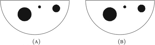
5.1. Example 1: Three balls, on-grid, no noise

In this initial example, we consider three balls of varying sizes. The centre points of the balls are within the set of 1093 grid points and there is no noise corrupting the boundary measurement generated from the solution, as shown in Figure 1(a). To solve this inverse problem the $L^2({\mathrm{\Gamma }}_M)$-norm is employed as the distance function. The method proposed finds three balls with the correct centre-points and radii with $2.7\times {10}^{-4}$%, $1.9\times {10}^{-4}$%, and $1.1\times {10}^{-4}$% error as shown in Figure 1(b). This demonstrates that in the ideal case, non-corrupted measurements and the centre points within the given set, the found balls match the target.

Figure 1. Example 1: Three balls, on-grid, no noise. (A) Target. (B) Result.

5.2. Example 2: One rectangle, on-grid, no noise

In this example we consider one 0.4 wide and 0.2 high rectangle which will be reconstructed as one and two balls. The centroid of the rectangle is within the set of 1093 grid points and there is no noise corrupting the boundary measurement generated from the solution, as shown in Figure 2. To solve this inverse problem all four error norms are employed as the distance function. The equivalent radius of the rectangle is defined as the radius of a circle with the same area. The method proposed first reconstructs the rectangular anomaly as one ball as shown in Figure 3. The resulting difference in centroid location and equivalent radius are listed in Table 1. This demonstrates that in the case that the target is not the assumed shape the equivalent centroid and area are reconstructed exactly for the $L^2(\mathrm{\Omega })$-norm, and close to this for the other error norms. Then the method reconstructs the rectangular anomaly as two balls as shown in Figure 3 and the error in compound centroid and equivalent radius is listed in Table 2. In this case the equivalent centroid and area are almost exactly reconstructed. The small error and lack of symmetry is likely due to the non-conforming mesh. However, it has shown in further examples that this method does not reconstruct more complex shapes well. It often fails with shapes such as an L-shaped anomaly.

Figure 2. Example 2: Rectangular target, no noise, on grid.

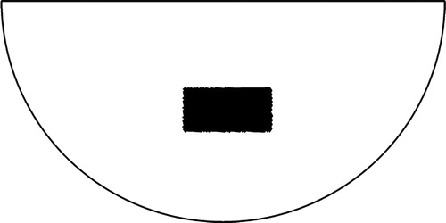
Figure 3. Example 2: Reconstruction of one rectangular target, no noise, on grid. (A) One ball. (B) Two balls.

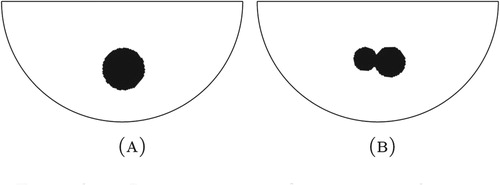
Table 1. Example 2: Error in constructing one rectangular target from one ball, no noise, on grid.

Distance function	$L^2({\mathrm{\Gamma }}_M)$-norm	$L^2(\mathrm{\Omega })$-norm	$H^1(\mathrm{\Omega })$-seminorm	$H^1(\mathrm{\Omega })$-norm
% Error in equivalent radius	9.0136	0.8125	9.0398	9.0361
Distance from rectangle's centroid to ball's centre	$6.94\times {10}^{-2}$	$1.03\times {10}^{-5}$	$6.94\times {10}^{-2}$	$6.94\times {10}^{-2}$

Table 2. Example 2: Error in constructing one rectangular target from two balls, no noise, on grid.

Distance function	$L^2({\mathrm{\Gamma }}_M)$-norm	$L^2(\mathrm{\Omega })$-norm	$H^1(\mathrm{\Omega })$-seminorm	$H^1(\mathrm{\Omega })$-norm
% Error in equivalent radius	0.1787	0.1783	0.1798	0.1797
Distance from rectangles' compound centroid to ball's centre	$4.13\times {10}^{-3}$	$4.11\times {10}^{-3}$	$4.16\times {10}^{-3}$	$4.16\times {10}^{-3}$

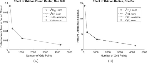
5.3. Example 3: One ball, no noise, with varying grid densities

In this example consider one ball with a radius of 0.1 where the centre point is not within the set of grid points, with no noise corrupting the boundary measurement, as shown in Figure 4. Here we consider grids with 79, 287, 1093, and 4665 points and all four distance functions. Based on the error in found centre and radius plotted in Figure 5, it is clear that as the grid is refined, regardless of distance function, the method converges towards a more accurate solution. Therefore, regardless of grid density or distance function, the found centre point is the closest to the true one. Also, it is shown that any error in centre point is compensated for by the radius of the ball.

Figure 4. Example 3: Target for one ball, no noise.

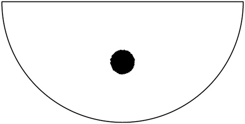
Figure 5. Example 3: Result for one ball, no noise, with varying grid densities.

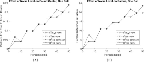
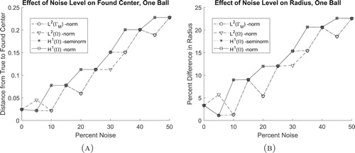
5.4. Example 4: One ball, on-grid, with varying levels of noise

In this example consider one ball where the centre point is within the set of 1093 grid points. Normally distributed random numbers, seeded with a value of one, are generated to act as noise. A varying per cent of this noise is then used to corrupt the target, which induces a corrupted boundary measurement. In particular, the target source $f^{\ast }$ is replaced by (42) $f_{\mu }^{\ast }(x)=f^{\ast }(x)+\mu \tau (x),$(42) where $\tau :\mathrm{\Omega }\mapsto \mathbb{R}$ is a random variable taking values in $(0,1)$ and μ corresponds to the noise level, as shown in Figure 6. Note that in this context, noisy data can be interpreted as modelling uncertainties. For each level of boundary measurement corruption, the error in found centre and radius is calculated for each distance function, as shown in Figure 7. These graphs demonstrate that, at larger percentages of noise, the $L^2$-norms tend to be more accurate. This is most likely due to the finite element integration.

Figure 6. Example 4: Target for one ball corrupted with varying levels of noise μ. (A) $\mu =5\mathrm{\%}$. (B) $\mu =10\mathrm{\%}$. (C) $\mu =15\mathrm{\%}$. (D) $\mu =20\mathrm{\%}$. (E) $\mu =25\mathrm{\%}$. (F) $\mu =30\mathrm{\%}$. (G) $\mu =35\mathrm{\%}$. (H) $\mu =40\mathrm{\%}$. (I) $\mu =45\mathrm{\%}$. (J) $\mu =50\mathrm{\%}$.

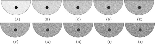
Figure 7. Example 4: Result for one ball, on-grid, with varying levels of noise.

5.5. Example 5: One ball, off-grid, with varying levels of noise

This experiment is the same as Example 4, except the centre point of the ball is not within the set of grid points. From Figure 8, similar to Example 3, it is shown that the inverse problem solution tends to be more resistant to noise when the $L^2$-norms are used as the distance functions. This difference seems to be more significant when the centre point is not contained within the set of grid points.

Figure 8. Example 5: Result for one ball, off-grid, with varying levels of noise.

6. Conclusions

In this paper, we consider the inverse source problem from a partial boundary measurement of the associated potential. This inverse problem is nonlinear and ill-posed [42]. The physical motivation of this problem comes from gravimetry such as the reconstruction of the mass density distribution of small regions of Earth, located close to its surface. Following the approach introduced in [6], we have proposed a non-iterative reconstruction method to detect the salient features of the hidden anomalies, such as the location, the size, the shape and the number, but without using the Newtonian potential to complement the unavailable information about the hidden boundary. In this setting, the inverse problem becomes more difficult to be solved, so that non-ball shaped anomalies are hard to reconstruct. The proposed approach is based on the Kohn–Vogelius formulation and the topological derivative method. The inverse source problem has been reformulated as a topology optimization problem. A second-order topological sensitivity is derived for different error norms. In particular, four examples of the Kohn–Vogelius functional are considered, namely $L^2({\mathrm{\Gamma }}_M)$-norm, $L^2(\mathrm{\Omega })$-norm, $H^1(\mathrm{\Omega })$-seminorm and $H^1(\mathrm{\Omega })$-norm of the error function. The second-order topological sensitivity has been used to devise a fast Newton-type reconstruction algorithm based on a simple optimization step. Finally, we have presented an extensive set of numerical experiments. First, the validity of the method is demonstrated and then the robustness of four different cost functions are compared. It is shown that although in theory the cost functions are identical, due to the discretization technique the $L^2$-norms tend to be more robust with respect to noise.

Acknowledgments

This research was partly supported by CNPq (Brazilian Research Council), CAPES (Brazilian Higher Education Staff Training Agency) and FAPERJ (Research Foundation of the State of Rio de Janeiro). The support is gratefully acknowledged.

Disclosure statement

No potential conflict of interest was reported by the author(s).

Additional information

Funding

This research was partly supported by CNPq (Brazilian Research Council), CAPES (Brazilian Higher Education Staff Training Agency) and FAPERJ (Research Foundation of the State of Rio de Janeiro).

References

- El Badia A, Ha-Duong T. An inverse source problem in potential analysis. Inverse Probl. 2000;16(3):651–663.
- Hettlich F, Rundell W. Iterative methods for the reconstruction of an inverse potential problem. Problems¡/DIFdel¿Inverse Probl. 1996;12(3):251.
- Isakov V. Inverse problems for partial differential equations. New York: Springer; 2006. (Applied Mathematical Sciences; 127).
- Liu J-C. An inverse source problem of the poisson equation with cauchy data. Electron J Differ Eq. 2017;2017(119):1–19.
- Canelas A, Laurain A, Novotny AA. A new reconstruction method for the inverse potential problem. J Comput Phys. 2014;268:417–431.
- Canelas A, Laurain A, Novotny AA. A new reconstruction method for the inverse source problem from partial boundary measurements. Inverse Probl. 2015;31(7):075009.
- Kohn R, Vogelius M. Relaxation of a variational method for impedance computed tomography. Commun Pure Appl Math. 1987;40(6):745–777.
- Novotny AA, Sokołowski J. Topological derivatives in shape optimization. Berlin: Springer-Verlag; 2013. (Interaction of Mechanics and Mathematics).
- Wexler A, Fry B, Neuman MR. Impedance-computed tomography algorithm and system. Appl Opt. 1985;24(23):3985–3992.
- Ben Abda A, Hassine M, Jaoua M, et al. Topological sensitivity analysis for the location of small cavities in stokes flow. SIAM J Control Optim. 2009;48:2871–2900.
- Hrizi M, Hassine M, Malek R. A new reconstruction method for a parabolic inverse source problem. Appl Anal. 2019;98(15):2723–2750.
- Schumacher A. Topologieoptimierung von Bauteilstrukturen unter Verwendung von Lochpositionierungskriterien [PhD thesis]. Forschungszentrum für Multidisziplinäre Analysen und Angewandte Strukturoptimierung. Institut für Mechanik und Regelungstechnik; 1996.
- Sokołowski J, Żochowski A. On the topological derivative in shape optimization. SIAM J Control Optim. 1999;37(4):1251–1272.
- Céa J, Garreau S, Guillaume Ph, et al. The shape and topological optimizations connection. Comput Methods Appl Mech Eng. 2000;188(4):713–726.
- Amstutz S, Horchani I, Masmoudi M. Crack detection by the topological gradient method. Control Cybernet. 2005;34(1):81–101.
- Bonnet M. Higher-order topological sensitivity for 2-D potential problems. Int J Solids Struct. 2009;46(11–12):2275–2292.
- Canelas A, Novotny AA, Roche JR. A new method for inverse electromagnetic casting problems based on the topological derivative. J Comput Phys. 2011;230:3570–3588.
- Caubet F, Dambrine M. Localization of small obstacles in stokes flow. Inverse Probl. 2012;28(10):1–31.
- Rocha de Faria J, Lesnic D. Topological derivative for the inverse conductivity problem: a Bayesian approach. J Sci Comput. 2015;63(1):256–278.
- Feijóo GR. A new method in inverse scattering based on the topological derivative. Inverse Probl. 2004;20(6):1819–1840.
- Allaire G, de Gournay F, Jouve F, et al. Structural optimization using topological and shape sensitivity via a level set method. Control Cybernet. 2005;34(1):59–80.
- Amstutz S, Andrä H. A new algorithm for topology optimization using a level-set method. J Comput Phys. 2006;216(2):573–588.
- Amstutz S, Novotny AA, de Souza Neto EA. Topological derivative-based topology optimization of structures subject to Drucker-Prager stress constraints. Comput Methods Appl Mech Eng. 2012;233–236:123–136.
- Garreau S, Guillaume Ph, Masmoudi M. The topological asymptotic for PDE systems: the elasticity case. SIAM J Control Optim. 2001;39(6):1756–1778.
- Auroux D, Masmoudi M, Belaid L. Image restoration and classification by topological asymptotic expansion. In: Taroco E, de Souza Neto EA, Novotny AA, editors. Variational formulations in mechanics: theory and applications. Barcelona: CIMNE; 2007. p. 23–42..
- Belaid LJ, Jaoua M, Masmoudi M, et al. Application of the topological gradient to image restoration and edge detection. Eng Anal Bound Elem. 2008;32(11):891–899.
- Hintermüller M. Fast level set based algorithms using shape and topological sensitivity. Control Cybernet. 2005;34(1):305–324.
- Hintermüller M, Laurain A. Multiphase image segmentation and modulation recovery based on shape and topological sensitivity. J Math Imaging Vis. 2009;35:1–22.
- Allaire G, Jouve F, Van Goethem N. Damage and fracture evolution in brittle materials by shape optimization methods. J Comput Phys. 2011;230(12):5010–5044.
- Xavier M, Fancello EA, Farias JMC, et al. Topological derivative-based fracture modelling in brittle materials: a phenomenological approach. Eng Fract Mech. 2017;179:13–27.
- Ammari H, Kang H, Lee H, et al. Boundary perturbations due to the presence of small linear cracks in an elastic body. J Elast. 2013;113:75–91.
- Van Goethem N, Novotny AA. Crack nucleation sensitivity analysis. Math Methods Appl Sci. 2010;33(16):1978–1994.
- Fernandez L, Novotny AA, Prakash R. Noniterative reconstruction method for an inverse potential problem modeled by a modified Helmholtz equation. Numer Funct Anal Optim. 2018;39(9):937–966. doi:10.1080/01630563.2018.1432645
- Ferreira AD, Novotny AA. A new non-iterative reconstruction method for the electrical impedance tomography problem. Inverse Probl. 2017;33(3):035005.
- Machado TJ, Angelo JS, Novotny AA. A new one-shot pointwise source reconstruction method. Math Methods Appl Sci. 2017;40(15):1367–1381.
- Rocha SS, Novotny AA. Obstacles reconstruction from partial boundary measurements based on the topological derivative concept. Struct Multidiscipl Optim. 2017;55(6):2131–2141.
- Baumeister J, Leitão A. Topics in inverse problems. Rio de Janeiro: IMPA Mathematical Publications; 2005.
- Burger M. A level set method for inverse problems. Inverse Probl. 2001;17:1327–1356.
- Hintermüller M, Laurain A. Electrical impedance tomography: from topology to shape. Control Cybernet. 2008;37(4):913–933.
- Isakov V, Leung S, Qian J. A fast local level set method for inverse gravimetry. Commun Comput Phys. 2011;10(4):1044–1070.
- Tricarico P. Global gravity inversion of bodies with arbitrary shape. Geophys J Int. 2013;195(1):260–275.
- Isakov V. Inverse source problems. Providence (RI): American Mathematical Society; 1990.