A reduced-order modelling for real-time identification of damages in multi-layered composite materials

Abstract

This work is focused on the detection of interlayer damages in multi-layer composite materials, which use the inverse analysis approach based on the reduced-order models (ROMs). Direct problems including heat conduction through the solid and heat radiation to the space are solved by finite element method (FEM), and the solutions of transient nonlinear analysis are collected to build the snapshot data matrix. The Proper Orthogonal Decomposition (POD) method coupled with two surrogate models are utilized to construct a low dimensional model which can be used to rebuild physical fields. By minimizing the discrepancy of measured and simulated temperatures using ROMs, the optimal parameter values related to damages can be estimated efficiently. Results prove that an excellent estimation on the position of damages can be obtained in the multi-layer materials. The computational efficiency and solution accuracy of two ROMs are compared, which proves that the POD-Kriging method has faster convergence speed than the POD-RBF method, with the same fitness value. Moreover, noise analysis validates that two ROMs have similar stability, whereas the POD-Kriging method is easier to achieve convergence in this type of problems.

KEYWORDS:

• Damage detection
• reduced-order model
• nonlinear heat transfer inverse problem
• multi-layer materials
• Proper Orthogonal Decomposition

SUBJECT CLASSIFICATION CODE:

• 65L09

1. Introduction

Multi-layer materials are essential for practical applications. Therefore, it is critically important to detect cracks or other flaws in real time that can limit the service lifetime of these structures. Cracks were tested by non-destructive testing techniques such as ultrasonic methods, magnetic field methods and eddy-current methods [1–3]. However, these methods have some higher requirements or restrictions for the test environment, such as ultrasonic methods require high temperature probes and coupling agent; as for magnetic field methods, it is just feasible for ferromagnetic materials and magnetic powder will be degaussed in high temperature environment; in terms of eddy-current methods, it is only for surface or near surface inspection. Therefore, motivated by accurately detect the global damage of complex structures, the numerical methods for direct or inverse problems have been developed [4–6].

As a type of inverse problems, inverse heat conduction problems (IHCPs), exist in aerospace field such as the measurement of boundary conditions for reentry flight vehicle [6] or a scramjet combustor [7], designing of thermal protection systems[8] and other engineering fields [9,10]. However, inverse problems are generally ill-posed, and thus, each new problem can include challenges relating to existence, uniqueness, and stability. The traditional way for solving inverse problems is to cast the inverse problem as an optimization problem. The results are obtained by repeating the global search and iteration, thus, it requires a lot of computing resources and very time-consuming. Several different techniques in references [11,12] could solve optimization problems and have been used in multilayered materials [13]. The techniques could be roughly divided into two categories, stochastic methods and gradient-based methods [14]. Compared with the gradient methods, the stochastic algorithm avoids local optimum to some extent. Genetic Algorithm (GA), one of the stochastic global optimal algorithms, was developed by reference to the natural selection and genetic evolution mechanism of living beings [15]. Individuals are created by three stochastic operations: selection, crossover and mutation. Thus, in order to improve computational efficiency while maintaining the excellent characteristics of random algorithms, the model reduction strategy is introduced into the calculation of inverse problem [16,17].

Reduced-order model (ROM), in particular the Proper Orthogonal Decomposition (POD) [18], combined with surrogate models [19] (e.g. Radial Basis Functions and Kriging interpolation), is an emerging technology that has been applied to different nondestructive material characterization problems, decreasing computational costs, and improving the inversion accuracy. The excellent feature of POD – utilizing a group of low-dimension characteristic bases to approximate the full-order models and guaranteeing the accuracy at the same time – makes it possible to reconstruct the physics field which then be applied into the parameters-identification problems [20–22]. One of the earliest groups of researchers who applied ROM to inverse problems was Ostrowski et al. [23,24]. They developed a ROM inverse approach to estimate the unknown heat conductivities and convective heat transfer coefficients in structures using POD combined with RBF. Since then, this kind of technique has been widely implemented in different fields, from material characterization, fluid flow, heat transfer and damage detection, among other fields [25–27].

To our best knowledge, few scholars compared differences between the two surrogate models combined with POD method in multi-layer materials, and few researchers applied this kind of method to the inversion of the high temperature multi-layer materials damage in the thermal protection system (TPS). Heat transfer through a multilayer medium during reentry into the atmosphere would involve combined modes of heat transfer: solid heat conduction, natural convection, and radiation interchange. In the present work, solid heat conduction and radiation interchange were considered, and natural convection was regarded as a type of boundary conditions which were imposed on the inside of the thermal protection layers. Based on the previous research in our team related to the inverse problem [7,14,28] and model reduction method [29–31], the purpose of this investigation is combining these two techniques to establish an more effective ROM for damage identification in multi-layer materials under high temperature environment.

The rest of this paper is organized as follows. Section 2 introduces the two-dimensional transient nonlinear heat conduction and radiation problem; the technical details of two ROMs (the POD technique and the surrogate model) are provided; In Section 3, the implementation of the proposed damage detection methodology are presented, including two numerical examples: a simple 2D steady heat conduction problem and a nonlinear transient heat conduction and radiation problem for a typical multilayer TPS. Results and noise analysis are also discussed in this section, in which the performance and accuracy are validated by comparing the results of the two ROMs. Finally, some conclusions are drawn in Section 4.

2. Fundamentals of two reduced-order models

2.1. Two-dimensional (2D) transient nonlinear heat conduction with a radiation boundary condition

The transient nonlinear heat conduction in each layer of composite material is modelled by using partial differential equations as follows: (1) $\rho C_p(T)\frac{\mathrm{\partial }T(x,y,t)}{\mathrm{\partial }t}=\frac{\mathrm{\partial }}{\mathrm{\partial }x}\left(k(T)\frac{\mathrm{\partial }T(x,y,t)}{\mathrm{\partial }x}\right)+\frac{\mathrm{\partial }}{\mathrm{\partial }y}\left(k(T)\frac{\mathrm{\partial }T(x,y,t)}{\mathrm{\partial }y}\right)$(1) where, T is the temperature; t is the time; C_p and k are the temperature-dependent specific heat and thermal conductivity, respectively; $\rho$ is the density. The associated initial condition is: (2) $T(x,y,t)|{}_{t=0}=T_0$(2) and boundary conditions are (3) $\begin{array}{rl}T|{}_{{\mathrm{\Gamma }}_1}& =T_a\end{array}$(3) (4) $\begin{array}{rl}-k(T)\frac{\mathrm{\partial }T(x,y,t)}{\mathrm{\partial }n}|{}_{{\mathrm{\Gamma }}_2}& =q_a(x,y,t)-\epsilon (T)B_o(T^4-{T_e}^4)\end{array}$(4) (5) $\begin{array}{rl}-k(T)\frac{\mathrm{\partial }T(x,y,t)}{\mathrm{\partial }n}|{}_{{\mathrm{\Gamma }}_3}& =h^{\ast }(T-T_e)\end{array}$(5)

in which, t=0 and T₀ are the initial time and temperature, respectively; T_a and $T_e$ are the applied and environment temperature; $B_o$ is the Boltzmann constant; $\epsilon$ is the emissivity of the external wall; q_a is the applied heat flux and h* is the heat convection coefficient; n is the unit outward normal to the boundary; .. represents the boundary of model, $\mathrm{\Gamma }={\mathrm{\Gamma }}_1\cup {\mathrm{\Gamma }}_2\cup {\mathrm{\Gamma }}_3$. Equation (1) subject to Equations (2)–(5) can be solved by means of the finite element method combined with specific problems and the detailed model description is introduced in the next part.

2.2. Proper Orthogonal Decomposition

Temperature field sets corresponding to different parameters are constructed by solving several direct nonlinear transient heat conduction problems. Each set of parameters corresponds to a snapshot (u) [32] proposed by Sirovich, and these snapshots are gathered in a rectangular N by L matrix $S=\{u_1,u_2,\dots ,u_L\}$ as a trained database which is a set of temperature fields containing N degrees of freedom for the L group of parameters $p=(p_1,p_2,\dots ,p_L)$. In the database, temperatures of boundary nodes are picked as input data. It is worth mentioning that the snapshot matrix S can be obtained either from a numerical model or from experiments. In this study, the solutions of direct problems have been obtained by numerical method and solved using the finite element method (FEM) by APDL codes. Subsequently, the trained database S will be used as the basis to build a ROM.

The essence of POD is to find a set of orthogonal vectors (bases) (6) $\mathrm{\Phi }=\{{\phi }_1,{\phi }_2,\dots ,{\phi }_L\}$(6)

Then, the response values of any nodes on the geometric model can be expressed as their linear combination. The mathematical statement of optimality is that the error norm for projection of each snapshot onto basis is equivalent to a constrained maximum problem, and this problem could also be considered as a largest eigenvalue problem, which can be written as: (7) $S{S}^{T}u=\lambda u$(7)

Considering matrix $S\in R^{N\times L}$, since $N>>L$, the dimension of matrix $S{S}^T$ is much larger than matrix $S^{T}S$, but their non-zero eigenvalues are exactly the same. Therefore, the correlation matrix $A$ is given by the following equation: (8) $A=S^{T}S$(8)

By solving the eigenvalues $\lambda$ and eigenvectors ${\psi }_i$ of $A$ (9) $A{\psi }_i={\lambda }_i{\psi }_{i}i=1,2,\dots ,L$(9) the eigenvectors ${\phi }_i$ of matrix $S{S}^T$ can be obtained by equation (10) ${\phi }_i=\frac{1}{\sqrt{{\lambda }_i}}S{\psi }_{i}i=1,2,\dots ,L$(10) Also, a group of POD bases are obtained. Therefore, the response values of any node on the geometric model could be expressed as: (11) $u(x,p,t)=\sum _{i=1}^L{\phi }_i(x){\alpha }_i(p,t)\text{ or }S=\mathrm{\Phi }\alpha$(11) where ${\alpha }_i$ represents the coefficients of POD bases correspond to parameters, called amplitude matrix. The linear relationship between snapshot matrix under different parameters and POD bases is established. Strictly, Equation (11) only applies to snapshots used to build the bases. However, since the snapshot matrix can reflect a specific physical field, in reality, the relationship between this particular physical field and other parameters can be utilized to construct an arbitrary snapshot matrix. Therefore, different physical fields correspond to different coefficients when the bases are known and $\alpha$ could be expressed as: (12) $\alpha ={\mathrm{\Phi }}^{T}S$(12)

Using POD bases to reduce the scale of the model can be achieved by truncating the number of bases. The eigenvalues corresponding to the bases need to be arranged in descending order. If the unknown quantity to be solved is the velocity, then the i-th eigenvalue can measure the kinetic energy reflected by the i-th POD bases [33]. As the number of bases increases, energy will drop rapidly. Choosing the first K bases that reflect the main energy can approximate the overall energy. Then ratio of the energy of a subspace to the energy of a full-order space is: (13) $I(K)=\frac{{\sum }_{i=1}^K{\lambda }_i}{{\sum }_{i=1}^L{\lambda }_i}$(13)

Full-order system could be projected to a lower-dimensional space using truncating POD bases because the ratio is close to 1. After truncating, the Equations (11) and (12) could be written as follows: (14) $\hat{\alpha }={\hat{\mathrm{\Phi }}}^{T}S$(14)

2.3. Surrogate model

The purpose of surrogate model is to establish the relationship between input and output data by training the model with samples and to give the best unbiased estimate of the output variables. Meanwhile, surrogate models aim to determine a continuous function (f) of a set of design variables from a limited amount of available data (f). In this work, surrogate model is not used to directly predict the unknown quantities but the coefficients of POD bases, for the purpose of avoiding the direct solution of a large number of unknowns but small scale coefficients, and then using POD for reduced-order analysis. Therefore, the relationship between unknown parameters and the whole physical field can be built. Identifying one parameter only needs L surrogate models if there are L POD bases. For parameters space $p=(p_1,p_2,\dots ,p_L)$, there are two different methods presented in this work.

2.3.1. POD-RBF based modelling

In POD-RBF [23,24] based surrogate model, the interpolation functions are defined as a series of functions using the Euclidean distance between unknown points and known points as their independent variables, called radial basis function. The amplitude matrix of ROM is constructed as follows: (15) ${\hat{\alpha }}_i(p)=B{f}_i(p)i=1,2,\dots ,L$(15) where, B is the coefficients matrix, and the f_i(p) is i-th interpolation function, usually the radial basis function being chosen. The common radial basis function can be found in the Ref [34].

In this work, the multiquadratic function is chosen as interpolation function, which is (16) $f_{ij}(p)=f({||p^j-p^i||}_2)=\sqrt{{||p^j-p^i||}_2+c^2}$(16) where $f_{ij}(p)$ are the factors of matrix $F(p)$; c is a user-defined smoothing factor to balance the relationship between ‘better interpolation' and ‘singularity'. It has proved that the flatness of the global shape function is important to increase the accuracy of the interpolation [35]. For multiquadratic RBF, as c goes to infinity, the shape function becomes flatter, and the approximation error goes to zero [35]. However, as c gets bigger, the matrix $F(p)$ will become singular. Taking these two aspects into consideration, the parameter c was chosen to be constant value 7. pⁱ and p^j correspond to the parameter vector of the i-th and j-th snapshot respectively. Therefore, equation (15) can be written in a matrix form as (17) $\hat{\alpha }(p)=\mathrm{B}F(p)$(17)

Combined with Equation (15), and then given a parameter space, a low-dimensional response space is obtained, that is (18) $\mathrm{B}=\hat{\alpha }(p)F(p{)}^{-1}{O}_1(p^{\mathrm{\prime }})=\hat{\mathrm{\Phi }}Bf(p^{\mathrm{\prime }})$(18) where O₁ represents the ROM1, $f(p^{\mathrm{\prime }})$ is a L-dimensional column vector whose value is related to the unknown point p’ and the known parameter space p.

2.3.2. POD-Kriging based modelling

The Kriging method showed a high performance in accuracy and robustness when adopted to obtain surrogates for different systems. To build an approximation for coefficients $\hat{\alpha }(p)$ of POD, the attractive features of Kriging are utilized as it offers a probabilistic framework. Unlike traditional Kriging, which estimates a single function as a target, the coefficients for each parameter need to be estimated, that is, a separate function for each interpolation vector have to be build. Therefore, L surrogate models are needed, which means the next process will be repeated L times. The Kriging model establishes a functional relationship of the following forms between input and output [36], (19) $\hat{\alpha }(p)=y^T(p)\beta +z(p)$(19) where,$y_i(p)(i=1,2,\dots ,L)$ are the regression functions. $\beta =\{{\beta }_1,{\beta }_2,\dots ,{\beta }_L{\}}^T$ $i,j=1,2,\dots ,L$ are the corresponding regression coefficients, and function $z(p)$ is a random process which has zero mean, a variance ${\sigma }_{}^2$, and a non-zero covariance: (20) $Var[z(p)]={\sigma }_z^2\text{ and }Cov[Z(p_i),Z(p_j)]={\sigma }_z^2[R_{ij}(\theta ,p_i,p_j)]$(20) where $Z=[z_1,z_2,\dots ,z_L{]}^T$, p_i and p_j represent any two points in the sample set. R is the correlation model with parameters $\theta$ and representing the space location between p_i and p_j. Meanwhile, R is a symmetric matrix and its diagonal element are 1. There is several choices for R such as Cubic spline, linear, Guassian or Spherical etc. The Gaussian correlation function is chosen in this work. Another correlational vector. $r(p)$ is introduced and it is a vector of correlations between design sites and untried point p’, as follows (21) $r(\theta ,p^{\mathrm{\prime }})=[R(\theta ,p_1,p^{\mathrm{\prime }}),R(\theta ,p_2,p^{\mathrm{\prime }}),\dots ,R(\theta ,p_L,p^{\mathrm{\prime }}){]}^T$(21) And the predictor can be found (22) $\begin{array}{rl}\hat{\alpha }(p^{\mathrm{\prime }})& =(r(p)-Yd{)}^T{R}^{-1}\alpha \end{array}$(22) (23) $\begin{array}{rl}{O}_2(p^{\mathrm{\prime }})& =\hat{\mathrm{\Phi }}\cdot \hat{\alpha }(p^{\mathrm{\prime }})\end{array}$(23) where $Y=[y_1,y_2,\dots ,y_L{]}^T$, $d=(Y^T{R}^{-1}Y{)}^{-1}(Y^T{R}^{-1}r-y)$ and $O_2(p^{\mathrm{\prime }})$ is the ROM2, a response space. Three unknown parameters,$\beta$, $\theta$ and ${\sigma }^2$, are undetermined currently. Normally, parameters are determined in order to choose correlation and regression functions. However, in practical terms, these two models need to be selected first, and then Kriging parameters can be determined via the provided statistical inference technique [37]. Therefore, an open software program called DACE [36] is used to obtain the parameters. Other than this, the correlation model and constant regression functions are built in this Matlab toolbox.

Using these two different methods to establish the relationship between arbitrary parameters in the parameter space and the physical field, this low-dimensional model is used to quickly reconstruct the original model, which lays the foundation for the subsequent damage identification.

2.4. Application of the genetic algorithm

The traditional way to solve inverse problems is using optimization algorithms. However, it could be impractical sometimes, because it requires solving the direct problem many times, with very high computational cost. Moreover, reduced-order models can be applied to directly utilize the relationship between the parameter space and the response space to quickly and accurately evaluate the optimal values during the inversion process.

During the process of parameters inversion, the optimization algorithm is one of the main technologies. In order to find optimal solutions, intelligent algorithms always show a big advantage since they avoid local optimum by global searching and the GA is used in this work. As a kind of random algorithms, GA also has the characteristics of global search, which greatly increases the calculation time as the whole model is required to analyze many times. Normally, long computational time for global searching gives a rise to the limit of GA, but since the ROMs are used to reduce the scale of calculation, the process is based on the ROMs and time for every single recalculation will be shortened. Therefore, the computational time is no longer the problem.

According to Section 2.3, the two ROMs can be constructed and referred as ROM 1 and ROM 2. The response values O₁ and O₂ are calculated from the trained POD model of the field Equations (18) and (23), respectively. 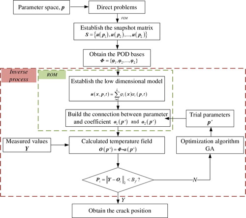The measured temperatures Y_i (i = 1,2, … ,m) as mentioned above can be utilized to generate the objective function that is built by the differences between measurements and calculated values, and the objective function is formed as: (24) ${\mathrm{P}}_i={\left|Y-O_i^{}\right|}_{2}j=1,2$(24) ${\mathrm{P}}_i$, the minimum value of the objective function, is sought, and the nonlinear least square problem can be solved by optimization algorithms. For clarity, the flow chart for the entire solution process is shown as Figure 1.

Figure 1. Flow chart of the reduced order inversion process.

3. Numerical examples

In this section, two numerical examples are calculated to verify the feasibility of the inverse crack identification methodology. The first example is a simple 2D steady heat conduction problem with two materials. The second example is a complicated practical problem, a thermal protection system with six layers, which is a nonlinear transient heat conduction with a radiation boundary condition. By identifying the position of the crack in these two different model and comparing the efficiency and accuracy using two ROMs, some conclusions are drawn. Additionally, this identification process is implemented by Matlab code, on a PC with Intel i7-4790 CPU of 3.60 GHz and RAM of 16GB.

3.1. Two materials cracked rectangular plate

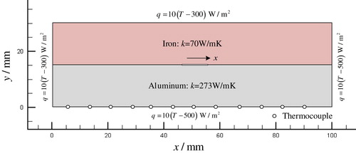
The first example is a 100 mm×30 mm 2D rectangular plate made of two materials, aluminum and iron (Figure 2), which is modelled by ANSYS software and APDL code. The entire plate is in a thermal environment and a crack (length of 5mm and thickness of 0.02mm) is assumed appears between two materials. Based in the fact that the parameters of the crack, i.e. position, changes the heat transfer behaviour, the variation of the temperature distribution is used to predict the crack parameters. The measured data in Equation (24) is detected by 19 thermocouples placed on the edge of the plate. The thermal environment of this model is as follows. The upper and left borders of the plate are convective boundary condition: $q=10(T-300)$ W/m²; the right and bottom borders of the plate are also the convective boundary condition: $q=10(T-500)$ W/m². In order to simulate flaws, contact resistance s_c which is a very small thermal conductivity for this heat conduction problem, is introduced at the location where the crack occur. At the interface between layers, thin layer with thickness of 0.02mm is reserved in advance. We assume that all cracks only occur in within the thin layer, interface thin layer is constructed and meshed. Therefore, when the position of the crack changes, there is no need to re-mesh and only the change of the element thermal conductivity to s_c which is close to zero at the corresponding location is needed. In this numerical example s_c = 1e-25. Finally, the model is meshed to 1680 quadrilateral elements and 1763 nodes.

Figure 2. Two materials cracked rectangular plate.

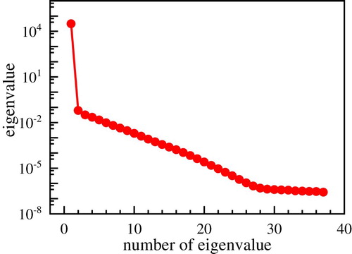
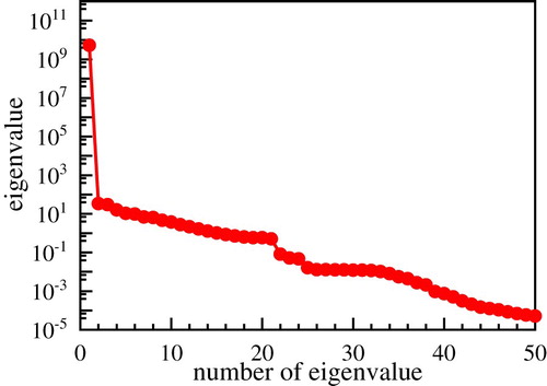
The crack can occur anywhere between the two materials. Therefore, we assume that the central position of the crack is changed from (c_x, c_y) = (5,15) to (95,15), and only the c_x coordinate should be identified. The range of the parameter is from 5 to 95 with uniform interval of 2.5. Direct problems are solved by commercial software ANSYS, which are used to generate the snapshot matrix S with a total of 37 snapshots. After building a database, the POD bases can be generated using Matlab codes, and their eigenvalues are shown in Figure 3. The values of eigenvalues sharply decrease with the increasing mode number, which means the first few bases contain the most energy of the system. Therefore, a truncated POD bases $\hat{\mathrm{\Phi }}$ consisting of 30 modes are established and these bases contain more than 99.99% energy of system.

Figure 3. The eigenvalues of POD basis.

The optimization algorithm GA is used to minimize the least square function for m=19 thermocouples and the parameters of GA are listed in the Table 1. The maximum number of generations is set to 5000, but if the fitness value satisfies B_f (a number close to zero), it is unnecessary to complete all the iterations.

Table 1. Parameters for GA.

Parameters	Values
Population size	20
Chromosome size	18
Cross rate	0.6
Mutate rate	0.8
Whether the elite choice	Yes

Two ROMs are used to reconstruct the temperature field according to the Equations (18) and (23), and the inversion process is to repeat this operation. Results are shown in Figure 4 plotting that the crack position converge to fitness values. For the ROM1, after 26 generations, the fitness value is obtained and for the ROM2, convergence is achieved after 19 steps. Correspondingly, the time spent are 0.27s and 0.15s for these two model, respectively. Table 2 shows the detailed values of estimated data and errors for two ROMs. From the convergence curve and results table, the performance of two ROMs is perfect. It should be noted that the ROM2 has a faster convergence speed and higher precision.

Figure 4. Evolution of the objective function.

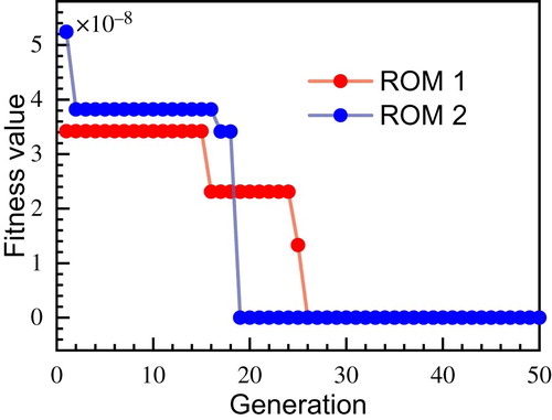
Table 2. Results of two ROMs for different sets of parameters.

	Estimated (mm)	Errors (%)	Time (s)	Generation	Bf
ROM1	50.3325	0.67	0.27	26	1.1e-8
ROM2	50.2199	0.44	0.15	19	1.1e-8

3.2. Multi-layered thermal protection system

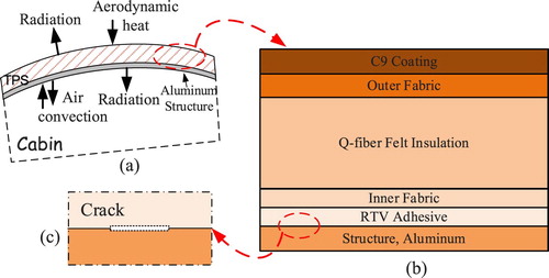
Thermal protection systems of aircrafts are built to protect its structures and onboard equipment from high temperature, especially during the atmospheric reentry phase. A typical multi-layer thermal protection structure, named Advanced Flexible Reusable Surface Insulation (AFRSI), has been applied on the U.S Space Shuttle orbiter [38] and used in place of white tiles in low-temperature areas for a long time and successfully flown on seven consecutive flights of the Space Shuttle Orbiter OV-099 [39] and performed well during the ascent and reentry. This TPS is selected as the validation object to test the reduced-order inversion algorithm presented not only because it represents a typical multi-layer TPS and can be easily transplanted to others, but also because it has the potential to be applied in the future, such as Space-Liner 7 [40]. Figure 5 shows the schematic diagram of the TPS structure. The TPS attached to the aluminum structure with RTV adhesive [41,42] is composed of an outer fabric with C9 coating, Q-fiber felt insulation, and an inner fabric layer. If there is a crack appeared between the layers, as shown in Figure 5(c), we hope to detect and locate delamination immediately without damaging the structure.

Figure 5. Cabin and its thermal protection system: (a) Cabin and the thermal environment; (b) multilayer TPS; (c) a crack between layers.

A 30 mm × 12.928mm 2D multi-layer plate model is constructed. The dimensions and boundary conditions are shown in Figure 6. For simulating this real-world problem, we reference some literatures to define the more realistic thermal environment [42,43], and the boundary conditions are as follows: the initial temperature is set as T₀ = 310K and the inner edge is assumed convective heat transfer and radiation boundary conditions: the cabin ambient temperature is a constant value of $T_e$ = 310K; heat transfer coefficient is assumed to be h* = 11.34 W/m²K and we suppose that TPS inner structure has a constant emissivity of ${\epsilon }_{in}$ = 0.6 (Temperature on the wall of the cabin(aluminum structure) being opposite to the TPS should be higher than that in the cabin). The aerodynamic heat flux history [42] on the outer surface along the trajectory is as shown in Figure 7. The radiation to the outer space is taken into account and the time-dependent emissivity is shown as Table A10 in the appendix. Other necessary temperature-dependent parameters, such as conductivity k(T), specific heat C_p(T) and density $\rho$ are also listed in the appendix, which are referenced from Ref. [41]. All the other boundaries are adiabatic. In order to verify the correctness of the model established and the rationality of boundary conditions imposed, the problem without cracks is solved by FEM and the temperature distribution at the central node in the outer surface is compared with that in Ref. [43], which is shown in Figure 8. As shown in Figure 8, the results are reasonable and the error is within 6.5%. Therefore, the model established is appropriate and realistic.

Figure 6. Computational model of multilayer TPS.

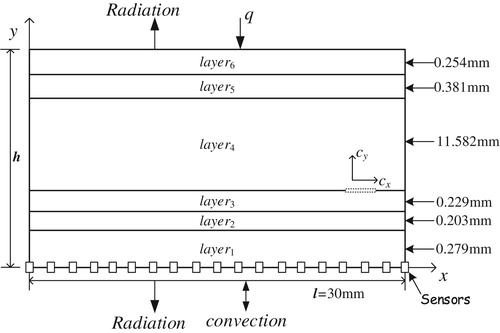
Figure 7. Heat flux history along the trajectory on X-34 windward.

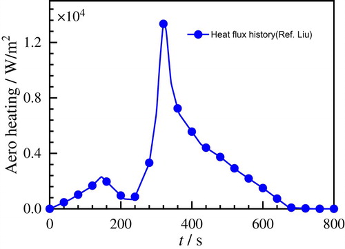
Figure 8. Outer surface temperature comparison of the present calculation results with those in Ref. [43].

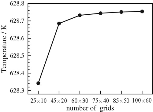
Assuming that a crack with a length of 1.2mm and a thickness of 0.04mm appears between layers, its coordinates are c_x and c_y which are also the parameters expected to be simultaneously identified. Temperature measurements at some accessible positions are necessary for the crack detecting. m thermocouples are placed at the inner surface of the thermal protection layers as shown in Figure 6, where the temperatures are easy to measure. Prior to detailed numerical investigation, a careful check for grid independence is carried out to ensure the accuracy and validity of the numerical method. When the calculation result does not change with the increase of the number of grids, the result is treated as a grid-independent solution. Six sets of computational meshes are checked: 25 × 10, 45 × 20, 60 × 30, 75 × 40, 85 × 50, 100 × 60 and the calculation results are shown in Figure 9. The results prove that the mesh set of 85 × 50 in vertical and horizontal directions, respectively, satisfies grid independence. Therefore, the model has 4250 quadratic elements and 4386 nodes.

Figure 9. Results with different meshes.

3.2.1. ROM for damage identification

Direct problems corresponding to different locations of crack are solved using FEM. APDL program codes are developed for automatic acquiring these direct problems results such as modelling and output of inner boundary temperature field. For the parameter space, c_x is changed from 6 to 24 with uniform interval of 1.2, and c_y={0.25233, 0.45533, 0.68433, 12.266, 12.647} are y-coordinate on the interface between the two materials. A total of 80 snapshots form a database and it takes the time of 21 minutes and 30 seconds. The eigenvalues are shown in Figure 10 and 50 POD modes are selected. The parameters of GA are listed in Table 1.

Figure 10. The eigenvalues of POD basis.

3.2.2. Results and discussion

After repeated calculations, the computing time of the full-order model is about 15s for one calculation (mainly depending on the time of meshing), while the time using the ROM will be only 0.01s in each calculation without re-meshing or model re-building. Furthermore, if the same number of iterations are needed during the inversion, the full-order model will take hundreds or even thousands of times more computational time than the ROM, which will make the detection non-real-time. As a result, use of ROM makes real time monitoring possible.

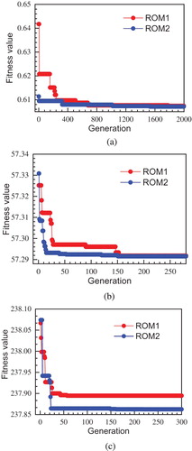
There are two groups of parameters as samples to verify that the inverse algorithm will be identified: (c_x, c_y)={(12.6, 0.68433), (8.4, 12.266)}, recorded as G1, G2, respectively. By identifying two groups of parameters which represent different locations of cracks between different layers, the accuracy and efficiency of two ROMs are compared. In the first case, between the inner fabric layer and the Q-fiber felt insulation layer, a crack located near the outer surface of the aircraft is identified, with the parameter (c_x, c_y) = (12.6, 0.68433). Results are illustrated in Table 3. ROM1 reaches convergence after 2411 generations, whereas ROM2 only needs 820 steps. Figure 11(a) shows the evolutionary process for fitness values, illustrating that ROM2 to ROM1 achieves a fast convergence value. As for the precisions of two parameters, c_x is within 0.5% (ROM1 is 0.46% and ROM2 is 0.38%); c_y is within 1% (ROM1 and ROM2 are both 0.67%). Both of two parameters can be detected very accurately, but in comparison, ROM2 has a faster recognition speed.

Figure 11. Evolution of the objective function for different group of parameters.

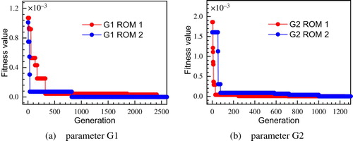
Table 3. Results of two ROMs for different sets of parameters.

	p	Estimated (mm)	Errors (%)	Time (s)	Generation	Bf
ROM1	cx	12.6275	0.46	8.76	2411	2e-5
	cy	0.6889	0.67
	cx	8.2544	1.73	5.33	1244	4e-5
	cy	12.2661	0.058
ROM2	cx	12.5519	0.38	1.91	820	2e-5
	cy	0.6889	0.67
	cx	8.4305	0.36	2.39	1001	4e-5
	cy	12.2589	0.058

A similar conclusion can be drawn from the second example. When the crack appears between the outer fabric layer and the Q-fiber felt insulation layer, the errors of the two models are 1.73%, 0.36% for c_x and both are 0.058% for c_y. In addition, the time spent are different, which are 5.33s and 2.39s for ROM1 and ROM2, respectively. It also proves that the ROM2 is easier to achieve convergence and the convergence curve is shown in Figure 11(b). These two examples illustrate POD method combined with surrogate models satisfies the accuracy requirements in the detection of multi-layer material damage and the POD-Kriging method is more efficient in this problem.

3.2.3. Noise analysis

In the above analysis, the temperature measurements are accurate and error-free. However, in actual measurement, random error is inevitable. Therefore, in order to study the stability of the ROM for crack identification in multi-layer materials with the presence of noise, an error term [28,44] is added to the exact temperature to account for the random measurement error. As shown in (25) (25) $T(c_x,c_y)=T(c_x,c_y{)}_{exact}(1+\zeta \eta /2.576)$(25) where $\eta$ is a normal distributed random variable, which is between −1 and 1. $\zeta$ is a measurement error at 99% confidence. The value of 2.576 occurs because 99% of a normal distributed population is between −2.576 and +2.576 standard deviation of the mean [44]. Parameter group G2 is used as an example to demonstrate the error effects on this model and 0.1%, 1%, 2% errors are now added into the exact temperatures. Simulated error values are shown in Figure 12. Then, the optimal algorithm GA is used to minimize the objective function, of which parameters are presented in Table 1. Similar to the previous error-free example, 18 thermocouples are located on the inside of the TPS but some errors are added in the measurement data. The results of identification are shown in Figure 13, which include the detected coordinates of a crack using different ROMs under various measurement errors. It appears that 0.1% noise has a little influence on the parameter c_x but c_y for both of ROM1 and ROM2. 1% noise has an influence on the parameter c_x and no significant effect on the parameter c_y. The slightly effect on parameter c_y can be eliminated since the structure of the material is known in advance and it is still possible to predict where the crack appears. The approximation error increases with the noise level, and when the noise level gets to 2%, both two parameters are affected. Furthermore, the evolutions of the objective function through GA are shown in Figure 14 with 0.1%, 1% and 2% errors, respectively. The iterative process is very fast and convergence could be obtained within 10s. It must be underlined that the ROM2 still shows a faster convergence rate compared to ROM1 even though there is some noise in the measured data. Even within a limited number of iterations, ROM2 will converge to a better value than ROM1 and this phenomenon will be more obvious when the noise becomes larger.

Figure 12. Measurement errors for different noise.

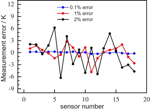
Figure 13. Estimated coordinates for different measurement errors using the two ROMs.

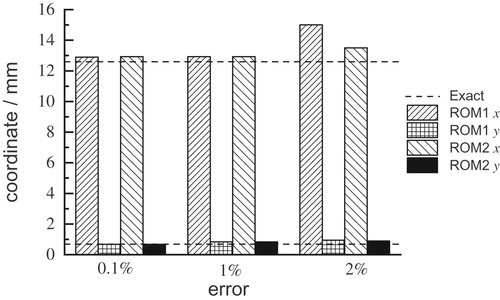
Figure 14. Evolution of the objective function with 0.1%, 1% and 2% error.

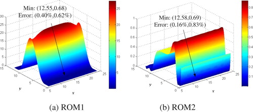
Furthermore, we calculated the values of objective function in the whole parameter space using the traversal method (c_x is from 6 to 24, c_y is from 0.2 to 12.9 and both of them with interval of 0.01. Even if the interval is not too small, it is still very costly) to find out the possible optimal value. Figure 15 shows the distribution of objective function values of ROM1 and ROM2. Even though these distribution do not cover every point in the parameter space, some meaningful conclusions can still be drawn. The minimum value of Equation (24) is marked on the figures: for ROM1 the optimal value is (12.55, 0.68) and for ROM2 is (12.58, 0.69); the errors for ROMs are (0.40%, 0.62%) and (0.16%, 0.83%), respectively. The errors are within 1%, but there are many similar points as shown in the figures. These similarities will affect the inversion accuracy with noise to some extent. Therefore, when the amplitude of noise is large (about 3% or more), this method definitely has a certain measurement error tolerance but it is limited and difficult to obtain a credible optimal value.

Figure 15. The distribution of objective function values using different ROMs.

4. Conclusions

In this work, a reduced-order model strategy is proposed by placing several thermocouples on the edge of the multi-layer material and applying numerical methods to identify the position of interlayer damage. By utilizing the powerful feature of POD model (the ability to represent the main characteristics of the original system solution using relatively few degrees of freedom) combined with two surrogate methods, RBF and Kriging methods, different reduced-order models are constructed to detect the parameters efficiently. Results show that the proposed techniques have the ability to accurately inverse the crack locations with a small computational cost and own a certain measurement error tolerance. In addition, the comparison between two ROMs illustrates that the POD-Kriging model is more efficient and has a faster convergence speed while maintaining accuracy in this problem. Moreover, it should be noted that although this method has a certain measurement error tolerance, we find that there are many similar points near the optimal value by roughly traversing the parameter space. In addition, GA has a certain randomness, which brings great difficulties to the detection of noise-involved problems. In this case, the similarity may be avoided by changing the objective function, narrowing the parameter range and averaging multiple computations.

Acknowledgements

The authors gratefully acknowledge the financial support for this research provided by the National Natural Science Foundation of China (Grant Nos. 11672061, 11972216, 11602129).

Disclosure statement

No potential conflict of interest was reported by the author(s).

Additional information

Funding

The work was financially supported by National Natural Science Foundation of China [grant numbers 11672061, 11972216, 11602129].

Appendix. Material properties

Table A1. Physical properties of different materials appearing in this paper.

	Aluminum	RTV	AB312	Q-fiber felt insulation	C9 coating
Density $\rho$ (kg/m^3)	2803.5	1409.8	985.13	96.12	2002.5
Conductivity k (W/mK)	200	Table A3	Table A5	Table A7	1.25
Specific heat $C_p$ (J/(kg.K))	Table A2	Table A4	Table A6	Table A8	Table A9
Emissivity $\epsilon$	–	–	–	–	Table A10

Table A2. Temperature (K)-dependent specific heat, $C_p$ (J/(kg.K)) for aluminum.

T	88	255	367	421	476
Cp	740.62	816.56	904.86	938.41	975.50

Table A3. Temperature (K)-dependent conductivity, k (W/mK) for RTV.

T	48	107	168	289	407	468
k	0.403	0.433	0.425	0.347	0.282	0.253

Table A4. Temperature (K)-dependent specific heat, $C_p$(J/(kg.K)) for RTV.

T	177	200	226	255	310	367	476	554
Cp	1143.27	1130.91	1088.52	1109.71	1192.72	1256.29	1424.06	1424.06

Table A5. Temperature (K)-dependent conductivity, k (W/mK) for AB312.

T	404	527	766	1006	1245
k	0.06258	0.09139	0.12318	0.16788	0.23344

Table A6. Temperature (K)-dependent specific heat, $C_p$ (J/(kg.K)) for AB312.

T	479	588	700	921	1142	1366	1478
Cp	844.81	933.11	987.86	1051.43	1092.05	1130.91	1152.10

Table A7. Temperature (K)-dependent conductivity, k (W/mK) for Q-fiber.

T	168	318	405	466	616	766	916	1064
k	0.033	0.052	0.063	0.071	0.091	0.114	0.138	0.165

Table A8. Temperature-dependent specific heat, $C_p$ (J/(kg.K)) for Q-fiber.

T	389	500	611	722	833	944	1167
Cp	845.82	975.63	1055.18	1117.99	1147.30	1172.43	1189.18

Table A9. Temperature (K)-dependent specific heat, $C_p$ (J/(kg.K)) for C9.

T	256	394	533	672	811	950	1089	1172	1367
Cp	741.1	887.7	1021.7	1130.6	1159.9	1126.4	1180.8	1235.2	1285.5

Table A10. Temperature (K)-dependent emissivity, $\epsilon$ for C9 coating on AFRSI.

T	256	394	533	672	811	950	1089	1228	1367
$\epsilon$	0.87	0.84	0.81	0.71	0.66	0.59	0.54	0.47	0.45

References

- Kumar S, Mahto DG. Recent trends in industrial and other engineering applications of non destructive testing: a review. Soc Sci Electr Publ. 2016;157(12):1055–1065.
- Soleimanpour R, Ng CT. Locating delaminations in laminated composite beams using nonlinear guided waves. Eng Struct. 2017;131:207–219.
- Banks HT, Joyner ML, Wincheski B, et al. Real time computational algorithms for eddy-current-based damage detection. Inverse Probl. 2001;18(3):795.
- Zhou SY, Cheng XW, Peng MJ, et al. Analysis of fracture problems of airport pavement by improved element-free Galerkin method(in Chinese). Acta Phys Sin. 2017;66(12):34–41.
- Benaissa B, Hocine NA, Belaidi I, et al. Crack identification using model reduction based on proper orthogonal decomposition coupled with radial basis functions. Struct Multidiscip 2016;54(2):265–274.
- Qian WQ, He KF, Zhou Y. Estimation of surface heat flux for ablation and charring of thermal protection material. Heat Mass Transfer. 2016;52(7):1–7.
- Cui M, Mei J, Zhang BW, et al. Inverse identification of boundary conditions in a scramjet combustor with a regenerative cooling system. Appl Therm Eng. 2018;134:555–563.
- Kumar S, Mahulikar SP. Design of thermal protection system for reusable hypersonic vehicle using inverse approach. J Spacecraft Rockets. 2017;54(2):1–11.
- Reddy SR, Dulikravich GS. Simultaneous determination of spatially varying thermal conductivity and specific heat using boundary temperature measurements. Inverse Probl Sci En. 2019;27(11):1635–1649.
- Zhuo LJ, Lesnic D, Meng SH. Reconstruction of the heat transfer coefficient at the interface of a bi-material. Inverse Probl Sci En. 2020;28(3):374–401.
- Beck JV, Blackwell B, Clair CR. Inverse heat conduction: Ill-posed problems. New York: Wiley; 1985.
- Ozisik MN, Orlande HRB. Inverse Heat Transfer: Fundamentals and Applications. New York: Taylor & Francis; 2000.
- Mishra AK, Chakraborty S. Determination of layerwise material properties of composite plates using mixed numerical-experimental technique. Inverse Probl Sci En. 2019;27(10):1468–1497.
- Cui M, Zhao Y, Xu B, et al. Inverse analysis for simultaneously estimating multi-parameters of temperature-dependent thermal conductivities of an Inconel in a reusable metallic thermal protection system. Appl Therm Eng. 2017;125:480–488.
- Holland JH. Adaptation in natural and artificial system. New York: MIT Press; 1992.
- Sumith S, Sangam K, Kannan K, et al. Prediction of nonlinear viscoelastic behaviour of simulative soil for deep-sea sediment using a thermodynamically compatible model. Inverse Probl Sci En. 2020;28(6):777–795.
- Alexandrino PDSL, Gomes GF, Cunha SS. A robust optimization for damage detection using multiobjective genetic algorithm, neural network and fuzzy decision making. Inverse Probl Sci En. 2020;28(1):21–46.
- Lumley JL. Coherent structures in turbulence. In: RE Meyer, London: Academic Press; 1981. p. 215–242.
- Queipo NV, Haftka RT, Wei S, et al. Surrogate-based analysis and optimization. Prog Aerosp Sci. 2005;41(1):1–28.
- Winton C, Pettway J, Kelley CT, et al. Application of proper orthogonal decomposition (POD) to inverse problems in saturated groundwater flow. Adv Water Resour. 2011;34(12):1519–1526.
- Brigham JC, Aquino W. Inverse viscoelastic material characterization using POD reduced-order modeling in acoustic–structure interaction. Comput Method Appl. 2009;198(9–12):893–903.
- Hoang KC, Khoo BC, Liu GR, et al. Rapid identification of material properties of the interface tissue in dental implant systems using reduced basis method. Inverse Probl Sci En. 2013;21(8):1310–1334.
- Ostrowski Z, Białecki RA, Kassab AJ. Solving inverse heat conduction problems using trained POD-RBF network inverse method. Inverse Probl Sci En. 2008;16(1):39–54.
- Ostrowski Z, Białecki RA, Kassab AJ. Estimation of constant thermal conductivity by use of proper orthogonal decomposition. Comput Mech. 2005;37(1):52–59.
- Bolzon G, Talassi M. An effective inverse analysis tool for parameter identification of anisotropic material models. Int J Mech Sci. 2013;77(4):130–144.
- Gunes H, Cadirci S. Modeling and inverse design of convective heat transfer in a grooved channel using proper orthogonal decomposition. ASME Imece. 2009: 519–526.
- Rogers CA, Kassab AJ, Divo EA, et al. An inverse POD-RBF network approach to parameter estimation in mechanics. Inverse Probl Sci En. 2012;20(5):749–767.
- Cui M, Zhao Y, Xu BB, et al. A new approach for determining damping factors in Levenberg-Marquardt algorithm for solving an inverse heat conduction problem. Int J Heat Mass Tran. 2017;107:747–754.
- Liang Y, Zheng BJ, Gao XW, et al. Reduced order model analysis method via proper orthogonal decomposition for nonlinear transient heat conduction problems (in Chinese). Sci China-Phys Mech Astron. 2018;48:124603.
- Gao XW, Hu JX, Huang SZ. A proper orthogonal decomposition analysis method for multimedia heat conduction problems. J Heat Trans ASME. 2016;138(7):71301–71311.
- Hu JX, Zheng BJ, Gao XW. Reduced order model analysis method via proper orthogonal decomposition for transient heat conduction (in Chinese). Sci China Phys Mech Astron. 2015;45:14602.
- Sirovich L. Turbulence and the dynamics of coherent structures part I: coherent structures. Q Appl Math. 1986;45(3):561–571.
- Lumley L. Turbulence, coherent structures, dynamical systems, and symmetry. London: Cambridge University Press; 1998.
- Hamim SU, Singh RP. Taguchi-based design of experiments in training POD-RBF surrogate model for inverse material modelling using nanoindentation. Inverse Probl Sci En. 2016;25(3):363–381.
- Baxter BJC. The asymptotic cardinal function of the multiquadratic φ(r) = (r2 + c2)12as c→∞. Comput Math Appl. 1992;24(12):1–6.
- Report T. DACE - A Matlab Kriging Toolbox, Version 2.0, Technical Report.
- Mirzazadeh R, Eftekhar SA, Mariani S. Mechanical characterization of polysilicon MEMS: a hybrid TMCMC/POD-Kriging approach. Sensors Basel. 2018;18(4):1243.
- Mui D, Clancy HM. Development of a protective ceramic coating for shuttle orbiter advanced flexible reusable surface insulation (AFRSI). Vol. 63. Westerville: AMER CERAMIC SOC; 1984. p. 1478–1478.
- Sawko PM, Goldstein HE. Performance of uncoated AFRSI blankets during multiple space shuttle flights. Nasa Sti/recon Technical Report 1992, 92;1992.
- Bauer C, Garbers N, Sippel M. The SpaceLiner 7 – vehicle and rescue capsule. Nagoya; 2013.
- Myers DE, Martin JCJ, Blosser ML. Parametric weight comparison of advanced metallic, ceramic tile, and ceramic blanket thermal protection systems, NASA Langley Technical Report Server; 2000.
- Zhu XW, Zhao JQ, Zhu L, et al. Impact of cabin environment on thermal protection system of crew hypersonic vehicle. Acta Astronaut. 2016;122:287–293.
- Liu DD, Chen PC, Tang L, et al. Integrated hypersonic aerothermoelastic methodology for transatmospheric vehicle (TAV) thermal protection system (TPS) structural design and optimization, AFRL-VA-WP-TR-2002-3047; 2002.
- Liu LH, Tan HP, Yu QZ. Inverse radiation problem of sources and emissivities in one-dimensional semitransparent media. Int J Heat Mass Tran. 2001;44(1):63–72.