Recovering a time-dependent potential function in a time fractional diffusion equation by using a nonlinear condition

Abstract

In this paper, we deal with a nonlinear inverse problem for recovering a time-dependent potential term in a time fractional diffusion equation from an additional measurement in the form of integral over the space domain. By using the fixed point theorem, the existence, uniqueness, regularity and stability of the direct problem are proved. The uniqueness of the inverse problem is proved by the property of Caputo fractional derivative. Numerically, we employ the Levenberg–Marquardt method to find the approximate potential function. Some different type examples are presented to show the feasibility and efficiency of the proposed method.

Keywords:

• Fractional diffusion equation
• inverse problem time-dependent potential term
• uniqueness
• Levenberg–Marquardt method
• numerical example.

2010 Mathematics Subject Classification:

• Inverse Problems

1. Introduction

Let Ω be a bounded domain in ${\mathbb{R}}^d$ with sufficiently smooth boundary $\mathrm{\partial }\mathrm{\Omega }.$ Suppose $d\le 3$, consider the following time-fractional diffusion problem (1) $\begin{array}{ll}{\mathrm{\partial }}_{0+}^{\alpha }u(x,t)-\mathrm{\Delta }u(x,t)+m(t)n(x,t)u(x,t)=f(x,t),& x\in \mathrm{\Omega },0<t\le T,\\ u(x,0)=0,& x\in \mathrm{\Omega },\\ u(x,t)=0,& x\in \mathrm{\partial }\mathrm{\Omega },0<t\le T,\end{array}$(1) where ${\mathrm{\partial }}_{0+}^{\alpha }u(x,t)$ for $0<\alpha <1$ denotes the Caputo fractional left-sided derivative of order α with respect to t ${\mathrm{\partial }}_{0+}^{\alpha }u(x,t)=\frac{1}{\mathrm{\Gamma }(1-\alpha )}{\int }_0^t(t-s{)}^{-\alpha }\frac{\mathrm{\partial }u}{\mathrm{\partial }s}(x,s)\mathrm{d}s,$ in which $\mathrm{\Gamma }(\cdot )$ is the Gamma function and T>0 is a fixed final time.

If all function $m(t),n(x,t)$ and $f(x,t)$ are given appropriately, the problem (1(1) $\begin{array}{ll}{\mathrm{\partial }}_{0+}^{\alpha }u(x,t)-\mathrm{\Delta }u(x,t)+m(t)n(x,t)u(x,t)=f(x,t),& x\in \mathrm{\Omega },0<t\le T,\\ u(x,0)=0,& x\in \mathrm{\Omega },\\ u(x,t)=0,& x\in \mathrm{\partial }\mathrm{\Omega },0<t\le T,\end{array}$(1) ) is a direct problem. The inverse problem here is to determine the time-dependent potential term $m(t)$ based on problem (1(1) $\begin{array}{ll}{\mathrm{\partial }}_{0+}^{\alpha }u(x,t)-\mathrm{\Delta }u(x,t)+m(t)n(x,t)u(x,t)=f(x,t),& x\in \mathrm{\Omega },0<t\le T,\\ u(x,0)=0,& x\in \mathrm{\Omega },\\ u(x,t)=0,& x\in \mathrm{\partial }\mathrm{\Omega },0<t\le T,\end{array}$(1) ) and an additional condition (2) $R(t)={\int }_{\mathrm{\Omega }}{u}^2(x,t)\mathrm{d}x,0\le t\le T.$(2) The physical motivation for such an observation is that we have the average information of $u(x,t)$ in the spatial observation domain Ω, the readers are refereed to [1] and the references therein.

There are some publications on the direct problem for time fractional diffusion equations. Kubica and Yamamoto proved the unique existence of weak solution for a fractional diffusion equation with coefficients depending on spatial and time variables by the Banach fixed point theorem in [2]. Li and Yamamoto proved the unique continuation of solutions for a one dimensional anomalous diffusion equation in [3]. McLean et al. established the well-posedness of an initial-boundary value problem for a general class of linear time fractional, advection–diffusion–reaction equations by using novel energy methods, a fractional Gronwall inequality and several properties of fractional integrals in [4]. See also [5–8] for other time fractional diffusion equation.

About recovering the time-dependent potential term in a fractional diffusion equation, there have been several literatures. In one-dimensional case and higher dimensional case, Zhang [9, 10] has proved a uniqueness of the undetermined coefficient problem by introducing an operator and show its monotonicity. Fujishiro [11] proved the stability of a source or a potential term by the generalized Gronwall inequality. Sun [12] considered an inverse time-dependent potential term in a multi-terms time fractional diffusion equation from observations of the solution at an interior or an boundary point, and obtained the stability of inverse problems. About recovering the space-dependent potential term in a fractional diffusion equation, one can see [13–19]. On the determination of coefficients in fractional partial differential equations, one can see the papers [20–22] in handbook published recently. Other inverse problems, one can see [23, 24].

To our knowledge, there are no literatures to give the uniqueness of the inverse time-dependent potential term $m(t)$ by calculating of variations and the property of Caputo fractional derivative. In this study, we obtain the existence, uniqueness and some regularities of the solution for the direct problem. The uniqueness of the inverse problem is proved by the property of Caputo fractional derivative. Moreover, we use the Levenberg–Marquardt method to solve numerically the inverse problem. Four different type examples are presented to show the feasibility and efficiency of the proposed method.

The rest of this paper has the following structure. In Section 2, we present some preliminaries used in Section 3 and Section 4. In Section 3, we present the existence, uniqueness, regularity and stablity of the solution for the direct problem. We obtain the uniqueness result for the inverse time-dependent potential function problem in Section 4. In Section 5, we use the Levenberg–Marquardt method to find the approximate solution. Numerical results for four examples are provided in Section 6. Finally, we give a conclusion in Section 7.

2. Preliminary

Throughout this paper, we use the following definitions and propositions. The notation C is a generic constant which has a different value everywhere.

Definition 2.1

[25]

If $y\in L^1(0,T),$ then for $\alpha >0$ the Riemann-Liouville fractional left-sided integral $I_{0+}^{\alpha }y(t)$ of order α are defined by $I_{0+}^{\alpha }y(t)=\frac{1}{\mathrm{\Gamma }(\alpha )}{\int }_0^t\frac{y(s)\mathrm{d}s}{(t-s{)}^{1-\alpha }},0<t\le T.$

Lemma 2.2

[25]

If $\alpha ,\beta >0,$ then the equation $(I_{0+}^{\alpha }{I}_{0+}^{\beta }f)(t)=(I_{0+}^{\alpha +\beta }f)(t)$ is satisfied at almost every point $t\in [0,T]forf\in L^1(0,T).$

Lemma 2.3

[26]

For any function $v\in AC[0,T]$, i.e. v is absolutely continuous on $[0,T],$ the following equality takes place: $v(t){\mathrm{\partial }}_{0+}^{\alpha }v(t)=\frac{1}{2}{\mathrm{\partial }}_{0+}^{\alpha }{v}^2(t)+\frac{\alpha }{2\mathrm{\Gamma }(1-\alpha )}{\int }_0^t\frac{\mathrm{d}\xi }{(t-\xi {)}^{1-\alpha }}{\left({\int }_0^{\xi }\frac{v^{\prime }(\eta )\mathrm{d}\eta }{(t-\eta {)}^{\alpha }}\right)}^2,$ where $0<\alpha <1.$

Corollary 2.4

If $u\in AC([0,T];L^2(\mathrm{\Omega })),$ we have ${\mathrm{\partial }}_{0+}^{\alpha }(u(\cdot ,t),u(\cdot ,t))\le 2({\mathrm{\partial }}_{0+}^{\alpha }u(\cdot ,t),u(\cdot ,t)),$ where $(\cdot ,\cdot )$ is the inner product in $L^2(\mathrm{\Omega })$ space.

Definition 2.5

[26]

The Mittag–Leffler function is (3) $E_{\alpha ,\beta }(z)=\sum _{k=0}^{\mathrm{\infty }}\frac{z^k}{\mathrm{\Gamma }(\alpha k+\beta )},z\in \mathbb{C},$(3) where $\alpha >0$ and $\beta \in \mathbb{R}$ are arbitrary constants. The function $E_{\alpha ,\beta }(z)$ is an entire function, and thus the function $E_{\alpha ,\beta }(t)$ is real analytic for $t\in \mathbb{R}.$

Lemma 2.6

[27]

Let $0<\alpha <2$ and $\beta \in \mathbb{R}$ be arbitrary. We suppose that μ is such that $\pi \alpha /2<\mu <min\{\pi ,\pi \alpha \}$. Then there exists a positive constant $C=C(\alpha ,\beta ,\mu )>0$ such that (4) $\mid E_{\alpha ,\beta }(z)\mid \le \frac{C}{1+\mid z\mid },z\in \mathbb{C},\mu \le \mid \arg (z)\mid \le \pi .$(4)

Lemma 2.7

[28]

Let $f\in L^p(0,T)$ and $g\in L^q(0,T)$ with $1\le p,q\le \mathrm{\infty }$ and $1/p+1/q=1.$ Then the function $f\ast g$ defined by $(f\ast g)(t)={\int }_0^{t}f(t-s)g(s)\mathrm{d}s$ belong to $C[0,T]$ and satisfies $|(f\ast g)(t)|\le \Vert f{\Vert }_{L^p(0,t)}\Vert g{\Vert }_{L^q(0,t)},t\in [0,T].$

Lemma 2.8

[11]

Let $u,v\in H^2(\mathrm{\Omega })$ and $d\le 3.$ Then $uv\in H^2(\mathrm{\Omega })$ with the estimate $\Vert uv{\Vert }_{H^2(\mathrm{\Omega })}\le C\Vert v{\Vert }_{H^2(\mathrm{\Omega })}$ with C>0 depending on $\Vert u{\Vert }_{H^2(\mathrm{\Omega })}.$

Lemma 2.9

[29]

Let $C,\alpha >0$ and $u,\varsigma \in L^1(0,T)$ be nonnegative functions satisfying $u(t)\le C\varsigma (t)+C{\int }_0^t(t-s{)}^{\alpha -1}u(s)\mathrm{d}s,t\in (0,T).$ Then we have $u(t)\le C\varsigma (t)+C{\int }_0^t(t-s{)}^{\alpha -1}\varsigma (s)\mathrm{d}s,t\in (0,T).$

Proposition 2.10

[25]

let $0<\alpha <1$ and $\lambda >0,$ then we have $\frac{\mathrm{d}}{\mathrm{d}t}{E}_{\alpha ,1}(-\lambda t^{\alpha })=-\lambda t^{\alpha -1}{E}_{\alpha ,\alpha }(-\lambda t^{\alpha }),t>0.$

Lemma 2.11

Suppose $h\in C^1[0,T],h(0)=0,0<\alpha <1,\lambda >0,$ denote $\beta (t)={\int }_0^{t}h(s)(t-s{)}^{\alpha -1}{E}_{\alpha ,\alpha }(-\lambda (t-s{)}^{\alpha })\mathrm{d}s,t\in (0,T],$ and define $\beta (0)=0,$ then $\beta \in C^1[0,T].$

Proof.

By Lemma 2.7, we know $\beta \in C[0,T].$

By $h(0)=0$ and $\beta (t)={\int }_0^{t}h(s)(t-s{)}^{\alpha -1}{E}_{\alpha ,\alpha }(-\lambda (t-s{)}^{\alpha })\mathrm{d}s,$ we have ${\beta }_t(t)={\int }_0^t{h}_s(s)(t-s{)}^{\alpha -1}{E}_{\alpha ,\alpha }(-\lambda (t-s{)}^{\alpha })\mathrm{d}s,$ since $h\in C^1[0,T],$ by Lemma 2.7, we know ${\beta }_t\in C[0,T],$ thus $\beta \in C^1[0,T].$

3. Existence, uniqueness and regularity of solution for the direct problem

In this paper, we need the property of Caputo fractional derivative when we prove Theorem 4.1, so we need the regularity of solution $u\in C^1([0,T];H^2(\mathrm{\Omega })\cap H_0^1(\mathrm{\Omega })).$ Based on the fixed point method, we give the existence, uniqueness and regularity of solution $u\in C^1([0,T];H^2(\mathrm{\Omega })\cap H_0^1(\mathrm{\Omega }))$ for the direct problem (1(1) $\begin{array}{ll}{\mathrm{\partial }}_{0+}^{\alpha }u(x,t)-\mathrm{\Delta }u(x,t)+m(t)n(x,t)u(x,t)=f(x,t),& x\in \mathrm{\Omega },0<t\le T,\\ u(x,0)=0,& x\in \mathrm{\Omega },\\ u(x,t)=0,& x\in \mathrm{\partial }\mathrm{\Omega },0<t\le T,\end{array}$(1) ).

Theorem 3.1

Let $m\in C^1[0,T]$, $n\in C^1([0,T];H^2(\mathrm{\Omega }))$ and $f\in C^1([0,T];H^2(\mathrm{\Omega })\cap H_0^1(\mathrm{\Omega }))$ such that $f(x,0)=0$. Then there exists a unique solution $u\in C^1([0,T];H^2(\mathrm{\Omega })\cap H_0^1(\mathrm{\Omega }))$ to (1(1) $\begin{array}{ll}{\mathrm{\partial }}_{0+}^{\alpha }u(x,t)-\mathrm{\Delta }u(x,t)+m(t)n(x,t)u(x,t)=f(x,t),& x\in \mathrm{\Omega },0<t\le T,\\ u(x,0)=0,& x\in \mathrm{\Omega },\\ u(x,t)=0,& x\in \mathrm{\partial }\mathrm{\Omega },0<t\le T,\end{array}$(1) ) such that $\mathrm{\Delta }u\in C^1([0,T];H^{2\gamma }(\mathrm{\Omega }))\mathrm{and}{\mathrm{\partial }}_{0+}^{\alpha }u\in C^1([0,T];H^{2\gamma }(\mathrm{\Omega })),$ for $0\le \gamma <1-(d/4),\gamma \ne \frac{1}{4},1\le d\le 3.$ Moreover, we get (5) $\Vert u{\Vert }_{C^1([0,T];H^2(\mathrm{\Omega }))}+\Vert \mathrm{\Delta }u{\Vert }_{C^1([0,T];H^{2\gamma }(\mathrm{\Omega }))}+\Vert {\mathrm{\partial }}_{0+}^{\alpha }u{\Vert }_{C^1([0,T];H^{2\gamma }(\mathrm{\Omega }))}\le C\Vert f{\Vert }_{C^1([0,T];H^2(\mathrm{\Omega }))}$(5) with C>0 depending on $\alpha ,\mathrm{\Omega },T,\gamma ,\Vert m{\Vert }_{C^1[0,T]}$ and $\Vert n{\Vert }_{C^1([0,T];H^2(\mathrm{\Omega }))}.$

In order to prove Theorem 3.1, we consider the time fractional diffusion equation with more general data. (6) $\begin{array}{ll}{\mathrm{\partial }}_{0+}^{\alpha }v(x,t)-\mathrm{\Delta }v(x,t)+r(x,t)v(x,t)=H(x,t),& x\in \mathrm{\Omega },0<t\le T,\\ v(x,0)=0,& x\in \mathrm{\Omega },\\ v(x,t)=0,& x\in \mathrm{\partial }\mathrm{\Omega },0<t\le T.\end{array}$(6) We assume the following conditions hold (7) $\begin{array}{rl}& r\in C^1([0,T];H^2(\mathrm{\Omega })).\end{array}$(7) (8) $\begin{array}{rl}& H\in C^1([0,T];H^2(\mathrm{\Omega })\cap H_0^1(\mathrm{\Omega })),H(x,0)=0.\end{array}$(8) Let us consider the following intermediate result.

Lemma 3.2

Let (7(7) $\begin{array}{rl}& r\in C^1([0,T];H^2(\mathrm{\Omega })).\end{array}$(7) ) and (8(8) $\begin{array}{rl}& H\in C^1([0,T];H^2(\mathrm{\Omega })\cap H_0^1(\mathrm{\Omega })),H(x,0)=0.\end{array}$(8) ) hold. Then there exists a unique solution $v\in C^1([0,T];H^2(\mathrm{\Omega })\cap H_0^1(\mathrm{\Omega }))$ to (6(6) $\begin{array}{ll}{\mathrm{\partial }}_{0+}^{\alpha }v(x,t)-\mathrm{\Delta }v(x,t)+r(x,t)v(x,t)=H(x,t),& x\in \mathrm{\Omega },0<t\le T,\\ v(x,0)=0,& x\in \mathrm{\Omega },\\ v(x,t)=0,& x\in \mathrm{\partial }\mathrm{\Omega },0<t\le T.\end{array}$(6) ) such that $\mathrm{\Delta }v\in C^1([0,T];H^{2\gamma }(\mathrm{\Omega }))\mathrm{and}{\mathrm{\partial }}_{0+}^{\alpha }v\in C^1([0,T];H^{2\gamma }(\mathrm{\Omega })),$ for $0\le \gamma <1-(d/4),\gamma \ne \frac{1}{4},1\le d\le 3.$ Moreover, we get (9) $\Vert v{\Vert }_{C^1([0,T];H^2(\mathrm{\Omega }))}+\Vert \mathrm{\Delta }v{\Vert }_{C^1([0,T];H^{2\gamma }(\mathrm{\Omega }))}+\Vert {\mathrm{\partial }}_{0+}^{\alpha }v{\Vert }_{C^1([0,T];H^{2\gamma }(\mathrm{\Omega }))}\le C\Vert H{\Vert }_{C^1([0,T];H^2(\mathrm{\Omega }))}$(9) with C>0 depending on $\alpha ,\mathrm{\Omega },T,\gamma$ and $\Vert r{\Vert }_{C^1([0,T];H^2(\mathrm{\Omega }))}.$

If we define $r(x,t)=m(t)n(x,t)$, then under the conditions for m and n in Theorem 3.1, the condition (7(7) $\begin{array}{rl}& r\in C^1([0,T];H^2(\mathrm{\Omega })).\end{array}$(7) ) is satisfied. Thus, we just have to verify Lemma 3.2.

Noting that $-\mathrm{\Delta }$ is a self-adjoint and positive operator in $H^2(\mathrm{\Omega })\cap H_0^1(\mathrm{\Omega })$. We denote the eigenvalues of $-\mathrm{\Delta }$ as ${\lambda }_k$ and the corresponding eigenfunctions as $\{{\varphi }_k{\}}_{k=1}^{\mathrm{\infty }}\subset H^2(\mathrm{\Omega })\cap H_0^1(\mathrm{\Omega }),$ which means we have $-\mathrm{\Delta }{\varphi }_k={\lambda }_k{\varphi }_k.$ We set $0<{\lambda }_1\le {\lambda }_2\le {\lambda }_3\le \cdots$, $\underset{n\to \mathrm{\infty }}{lim}{\lambda }_n=\mathrm{\infty }$ and $\{{\varphi }_k{\}}_{k=1}^{\mathrm{\infty }}$ is an orthonormal basis in $L^2(\mathrm{\Omega })$. Define the Hilbert scale space $D((-\mathrm{\Delta }{)}^{\gamma })$ for $\gamma \ge 0$ (see [30]) by $\begin{array}{rl}D({(-\mathrm{\Delta })}^{\gamma })& =\{\psi \in L^2(\mathrm{\Omega });\sum _{k=1}^{\mathrm{\infty }}{\lambda }_k^{2\gamma }|(\psi ,{\varphi }_k){|}^2<\mathrm{\infty }\},\\ (-\mathrm{\Delta }{)}^{\gamma }\psi & =\sum _{k=1}^{\mathrm{\infty }}{\lambda }_k^{\gamma }(\psi ,{\varphi }_k){\varphi }_k,\psi \in D((-\mathrm{\Delta }{)}^{\gamma }),\end{array}$ where $(\cdot ,\cdot )$ is the inner product in $L^2(\mathrm{\Omega })$ space. Define its norm $\Vert \psi {\Vert }_{D((-\mathrm{\Delta }{)}^{\gamma })}=\Vert (-\mathrm{\Delta }{)}^{\gamma }\psi {\Vert }_{L^2(\mathrm{\Omega })}.$ According to [31, 32], we have (10) $\begin{array}{rl}& D(-\mathrm{\Delta }):=D((-\mathrm{\Delta }{)}^1)=H^2(\mathrm{\Omega })\cap H_0^1(\mathrm{\Omega }),\\ & D((-\mathrm{\Delta }{)}^{\gamma })\subset H^{2\gamma }(\mathrm{\Omega }),0\le \gamma \le 1,\end{array}$(10) (11) $\begin{array}{rl}& C_1\Vert \psi {\Vert }_{H^{2\gamma }}\le \Vert \psi {\Vert }_{D((-\mathrm{\Delta }{)}^{\gamma })}\le C_2\Vert \psi {\Vert }_{H^{2\gamma }},\psi \in D((-\mathrm{\Delta }{)}^{\gamma }),0\le \gamma \le 1,\gamma \ne \frac{1}{4},\frac{3}{4}.\end{array}$(11) We denote the operator valued function $P(t)$ by $P(t)\psi =\sum _{k=1}^{\mathrm{\infty }}(\psi ,{\varphi }_k)t^{\alpha -1}{E}_{\alpha ,\alpha }(-{\lambda }_k{t}^{\alpha }){\varphi }_k,\psi \in L^2(\mathrm{\Omega }),t>0,$ with the Mittag–Leffler function given by Definition 2.5. We can get $P\in L^1(0,T;B(L^2(\mathrm{\Omega }))),$ where $B(L^2(\mathrm{\Omega }))$ denotes the bounded linear operator in $L^2(\mathrm{\Omega }).$

From $(-\mathrm{\Delta }{)}^{\gamma }P(t)\psi =\sum _{k=1}^{\mathrm{\infty }}{\lambda }_k^{\gamma }(\psi ,{\varphi }_k)t^{\alpha -1}{E}_{\alpha ,\alpha }(-{\lambda }_k{t}^{\alpha }){\varphi }_k$ and Lemma 2.6, we can obtain (12) $\begin{array}{rl}& \Vert (-\mathrm{\Delta }{)}^{\gamma }P(t)\psi {\Vert }_{L^2(\mathrm{\Omega })}={(\sum _{k=1}^{\mathrm{\infty }}[{\lambda }_k^{\gamma }(\psi ,{\varphi }_k)t^{\alpha -1}{E}_{\alpha ,\alpha }(t){]}^2)}^{1/2}\\ & \le C{\left(\sum _{k=1}^{\mathrm{\infty }}{((\psi ,{\varphi }_k)\frac{{\lambda }_k^{\gamma }{t}^{\alpha -1}}{1+{\lambda }_k{t}^{\alpha }})}^2\right)}^{1/2}\\ & \le C{t}^{\alpha (1-\gamma )-1}\Vert \psi {\Vert }_{L^2(\mathrm{\Omega })}.\end{array}$(12) Consider the following initial boundary value problem (13) $\begin{array}{ll}{\mathrm{\partial }}_{0+}^{\alpha }w(x,t)-\mathrm{\Delta }w(x,t)=h(x,t),& x\in \mathrm{\Omega },0<t\le T,\\ w(x,0)=0,& x\in \mathrm{\Omega },\\ w(x,t)=0,& x\in \mathrm{\partial }\mathrm{\Omega },t\in (0,T].\end{array}$(13) By [8], we know that (13(13) $\begin{array}{ll}{\mathrm{\partial }}_{0+}^{\alpha }w(x,t)-\mathrm{\Delta }w(x,t)=h(x,t),& x\in \mathrm{\Omega },0<t\le T,\\ w(x,0)=0,& x\in \mathrm{\Omega },\\ w(x,t)=0,& x\in \mathrm{\partial }\mathrm{\Omega },t\in (0,T].\end{array}$(13) ) exists a unique solution provided by (14) $\begin{array}{rl}w(x,t)& ={\int }_0^{t}P(t-s)h(\cdot ,s)\mathrm{d}s\\ & =\sum _{k=1}^{\mathrm{\infty }}{\int }_0^t(h(\cdot ,s),{\varphi }_k)(t-s{)}^{\alpha -1}{E}_{\alpha ,\alpha }(-{\lambda }_k(t-s{)}^{\alpha })\mathrm{d}s{\varphi }_k(x).\end{array}$(14) By Proposition 2.10, we have (15) $\begin{array}{rl}\Vert w(\cdot ,t){\Vert }_{D(-\mathrm{\Delta })}& =\Vert -\mathrm{\Delta }w{\Vert }_{L^2(\mathrm{\Omega })}\\ & ={\left\{\sum _{k=1}^{\mathrm{\infty }}{[{\int }_0^t{\lambda }_k(h(\cdot ,s),{\varphi }_k)(t-s{)}^{\alpha -1}{E}_{\alpha ,\alpha }(-{\lambda }_k(t-s{)}^{\alpha })\mathrm{d}s]}^2\right\}}^{1/2}\\ & \le {\{\sum _{k=1}^{\mathrm{\infty }}\underset{0\le s\le T}{max}|{\lambda }_k{h}_k(s){|}^2{({\int }_0^t(t-s{)}^{\alpha -1}{E}_{\alpha ,\alpha }(-{\lambda }_k(t-s{)}^{\alpha })\mathrm{d}s)}^2\}}^{1/2}\\ & \le {\{\sum _{k=1}^{\mathrm{\infty }}\underset{0\le s\le T}{max}|{\lambda }_k{h}_k(s){|}^2\frac{C}{{\lambda }_k^2}\}}^{1/2}\end{array}$(15) where $h_k(s)=(h(\cdot ,s),{\varphi }_k{)}_{L^2(\mathrm{\Omega })}.$ By ${\lambda }_k=O(k^{2/d}),$ it yiel ds $\sum _{k=1}^{\mathrm{\infty }}\frac{1}{{\lambda }_k^2}<\mathrm{\infty }$ for $1\le d\le 3.$ Since $\underset{0\le s\le T}{max}|{\lambda }_k{h}_k(s){|}^2\le \underset{0\le s\le T}{max}\sum _{k=1}^{\mathrm{\infty }}{\lambda }_k^2{h}_k^2(s)=\Vert h{\Vert }_{C([0,T];D(-\mathrm{\Delta }))}^2,$ hence the series (15(15) $\begin{array}{rl}\Vert w(\cdot ,t){\Vert }_{D(-\mathrm{\Delta })}& =\Vert -\mathrm{\Delta }w{\Vert }_{L^2(\mathrm{\Omega })}\\ & ={\left\{\sum _{k=1}^{\mathrm{\infty }}{[{\int }_0^t{\lambda }_k(h(\cdot ,s),{\varphi }_k)(t-s{)}^{\alpha -1}{E}_{\alpha ,\alpha }(-{\lambda }_k(t-s{)}^{\alpha })\mathrm{d}s]}^2\right\}}^{1/2}\\ & \le {\{\sum _{k=1}^{\mathrm{\infty }}\underset{0\le s\le T}{max}|{\lambda }_k{h}_k(s){|}^2{({\int }_0^t(t-s{)}^{\alpha -1}{E}_{\alpha ,\alpha }(-{\lambda }_k(t-s{)}^{\alpha })\mathrm{d}s)}^2\}}^{1/2}\\ & \le {\{\sum _{k=1}^{\mathrm{\infty }}\underset{0\le s\le T}{max}|{\lambda }_k{h}_k(s){|}^2\frac{C}{{\lambda }_k^2}\}}^{1/2}\end{array}$(15) ) is uniformly convergent for $t\in [0,T]$, by Lemma 2.11, we know each term in (15(15) $\begin{array}{rl}\Vert w(\cdot ,t){\Vert }_{D(-\mathrm{\Delta })}& =\Vert -\mathrm{\Delta }w{\Vert }_{L^2(\mathrm{\Omega })}\\ & ={\left\{\sum _{k=1}^{\mathrm{\infty }}{[{\int }_0^t{\lambda }_k(h(\cdot ,s),{\varphi }_k)(t-s{)}^{\alpha -1}{E}_{\alpha ,\alpha }(-{\lambda }_k(t-s{)}^{\alpha })\mathrm{d}s]}^2\right\}}^{1/2}\\ & \le {\{\sum _{k=1}^{\mathrm{\infty }}\underset{0\le s\le T}{max}|{\lambda }_k{h}_k(s){|}^2{({\int }_0^t(t-s{)}^{\alpha -1}{E}_{\alpha ,\alpha }(-{\lambda }_k(t-s{)}^{\alpha })\mathrm{d}s)}^2\}}^{1/2}\\ & \le {\{\sum _{k=1}^{\mathrm{\infty }}\underset{0\le s\le T}{max}|{\lambda }_k{h}_k(s){|}^2\frac{C}{{\lambda }_k^2}\}}^{1/2}\end{array}$(15) ) is continuous on $[0,T],$ thus $w(x,t)\in C([0,T];D(-\mathrm{\Delta }))$. It is easy to prove $w(x,0)=0$ and obtain the following estimate $\Vert w{\Vert }_{C([0,T];D(-\mathrm{\Delta }))}\le C\Vert h{\Vert }_{C([0,T];D(-\mathrm{\Delta }))}.$

Note that $h(x,0)=0,$ by a simple calculate, we have $w_t(x,t)=\sum _{k=1}^{\mathrm{\infty }}{\int }_0^t(h_s(\cdot ,s),{\varphi }_k)(t-s{)}^{\alpha -1}{E}_{\alpha ,\alpha }(-{\lambda }_k(t-s{)}^{\alpha })\mathrm{d}s{\varphi }_k(x).$ Similar to the proof in (15(15) $\begin{array}{rl}\Vert w(\cdot ,t){\Vert }_{D(-\mathrm{\Delta })}& =\Vert -\mathrm{\Delta }w{\Vert }_{L^2(\mathrm{\Omega })}\\ & ={\left\{\sum _{k=1}^{\mathrm{\infty }}{[{\int }_0^t{\lambda }_k(h(\cdot ,s),{\varphi }_k)(t-s{)}^{\alpha -1}{E}_{\alpha ,\alpha }(-{\lambda }_k(t-s{)}^{\alpha })\mathrm{d}s]}^2\right\}}^{1/2}\\ & \le {\{\sum _{k=1}^{\mathrm{\infty }}\underset{0\le s\le T}{max}|{\lambda }_k{h}_k(s){|}^2{({\int }_0^t(t-s{)}^{\alpha -1}{E}_{\alpha ,\alpha }(-{\lambda }_k(t-s{)}^{\alpha })\mathrm{d}s)}^2\}}^{1/2}\\ & \le {\{\sum _{k=1}^{\mathrm{\infty }}\underset{0\le s\le T}{max}|{\lambda }_k{h}_k(s){|}^2\frac{C}{{\lambda }_k^2}\}}^{1/2}\end{array}$(15) ), we have $w_t(x,t)\in C([0,T];D(-\mathrm{\Delta })),$ thus $w(x,t)\in C^1([0,T];D(-\mathrm{\Delta })).$ And also get (16) $\Vert w_t{\Vert }_{C([0,T];D(-\mathrm{\Delta }))}\le C\Vert h_t{\Vert }_{C([0,T];D(-\mathrm{\Delta }))}.$(16) By the generalized Minkowski inequality, we have $\begin{array}{rl}\Vert w(\cdot ,t){\Vert }_{D(-\mathrm{\Delta })}& \le {\int }_0^t\Vert P(t-s)h(\cdot ,s){\Vert }_{D(-\mathrm{\Delta })}\mathrm{d}s\\ & \le {\int }_0^t{(\sum _{k=1}^{\mathrm{\infty }}{\lambda }_k^2(h(\cdot ,s),{\varphi }_k{)}^2(t-s{)}^{2\alpha -2}{E}_{\alpha ,\alpha }^2(-{\lambda }_k(t-s{)}^{\alpha }))}^{1/2}\mathrm{d}s\\ & \le C{\int }_0^t(t-s{)}^{\alpha -1}{(\sum _{k=1}^{\mathrm{\infty }}{\lambda }_k^2(h(\cdot ,s),{\varphi }_k{)}^2)}^{1/2}\mathrm{d}s\\ & \le \frac{C{t}^{\alpha }}{\alpha }\underset{s\in [0,T]}{max}{(\sum _{k=1}^{\mathrm{\infty }}{\lambda }_k^2(h(\cdot ,s),{\varphi }_k{)}^2)}^{1/2}\\ & =\frac{C{t}^{\alpha }}{\alpha }\Vert h{\Vert }_{C([0,T];D(-\mathrm{\Delta }))}.\end{array}$ Similarly, we can obtain $\Vert w_t(\cdot ,t){\Vert }_{D(-\mathrm{\Delta })}\le \frac{C{t}^{\alpha }}{\alpha }\Vert h_t{\Vert }_{C([0,T];D(-\mathrm{\Delta }))}.$ Denote $X=\{v\in C^1([0,T];D(-\mathrm{\Delta })),v(x,0)=0\}.$

Here we define the map $L:X\to X$ as (17) $(Lh)(x,t)={\int }_0^{t}P(t-s)h(\cdot ,s)\mathrm{d}s,h\in X.$(17) Therefore, we have (18) $\Vert Lh{\Vert }_{C^1([0,T];D(-\mathrm{\Delta }))}\le C\Vert h{\Vert }_{C^1([0,T];D(-\mathrm{\Delta }))}.$(18) Next we give the proof of Lemma 3.2

Proof of Lemma 3.2.

The problem (6(6) $\begin{array}{ll}{\mathrm{\partial }}_{0+}^{\alpha }v(x,t)-\mathrm{\Delta }v(x,t)+r(x,t)v(x,t)=H(x,t),& x\in \mathrm{\Omega },0<t\le T,\\ v(x,0)=0,& x\in \mathrm{\Omega },\\ v(x,t)=0,& x\in \mathrm{\partial }\mathrm{\Omega },0<t\le T.\end{array}$(6) ) could be written as (19) $\begin{array}{ll}{\mathrm{\partial }}_{0+}^{\alpha }v(x,t)-\mathrm{\Delta }v(x,t)=-r(x,t)v(x,t)+H(x,t),& x\in \mathrm{\Omega },0<t\le T,\\ v(x,0)=0,& x\in \mathrm{\Omega },\\ v(x,t)=0,& x\in \mathrm{\partial }\mathrm{\Omega },t\in (0,T].\end{array}$(19) We see from (14(14) $\begin{array}{rl}w(x,t)& ={\int }_0^{t}P(t-s)h(\cdot ,s)\mathrm{d}s\\ & =\sum _{k=1}^{\mathrm{\infty }}{\int }_0^t(h(\cdot ,s),{\varphi }_k)(t-s{)}^{\alpha -1}{E}_{\alpha ,\alpha }(-{\lambda }_k(t-s{)}^{\alpha })\mathrm{d}s{\varphi }_k(x).\end{array}$(14) ) that the solution v of (19(19) $\begin{array}{ll}{\mathrm{\partial }}_{0+}^{\alpha }v(x,t)-\mathrm{\Delta }v(x,t)=-r(x,t)v(x,t)+H(x,t),& x\in \mathrm{\Omega },0<t\le T,\\ v(x,0)=0,& x\in \mathrm{\Omega },\\ v(x,t)=0,& x\in \mathrm{\partial }\mathrm{\Omega },t\in (0,T].\end{array}$(19) ) can be written as (20) $\begin{array}{rl}v(x,t)& ={\int }_0^t-P(t-s)r(\cdot ,s)v(\cdot ,s)\mathrm{d}s+{\int }_0^{t}P(t-s)H(\cdot ,s)\mathrm{d}s\\ & =\sum _{k=1}^{\mathrm{\infty }}{\int }_0^t(-r(\cdot ,s)v(\cdot ,s),{\varphi }_k)(t-s{)}^{\alpha -1}{E}_{\alpha ,\alpha }(-{\lambda }_k(t-s{)}^{\alpha })\mathrm{d}s{\varphi }_k(x)\\ & +\sum _{k=1}^{\mathrm{\infty }}{\int }_0^t(H(\cdot ,s),{\varphi }_k(x))(t-s{)}^{\alpha -1}{E}_{\alpha ,\alpha }(-{\lambda }_k(t-s{)}^{\alpha })\mathrm{d}s{\varphi }_k(x)\\ & =I_1+I_2.\end{array}$(20) By Lemma 2.8 and (7(7) $\begin{array}{rl}& r\in C^1([0,T];H^2(\mathrm{\Omega })).\end{array}$(7) ), we know that $rv\in C^1([0,T];D(-\mathrm{\Delta }))$ and (21) $\Vert r(\cdot ,t)v(\cdot ,t){\Vert }_{D(-\mathrm{\Delta })}\le C\Vert v(\cdot ,t){\Vert }_{D(-\mathrm{\Delta })},$(21) where C>0 is depending on $\Vert r{\Vert }_{C^1([0,T];D(-\mathrm{\Delta }))}.$

In (15(15) $\begin{array}{rl}\Vert w(\cdot ,t){\Vert }_{D(-\mathrm{\Delta })}& =\Vert -\mathrm{\Delta }w{\Vert }_{L^2(\mathrm{\Omega })}\\ & ={\left\{\sum _{k=1}^{\mathrm{\infty }}{[{\int }_0^t{\lambda }_k(h(\cdot ,s),{\varphi }_k)(t-s{)}^{\alpha -1}{E}_{\alpha ,\alpha }(-{\lambda }_k(t-s{)}^{\alpha })\mathrm{d}s]}^2\right\}}^{1/2}\\ & \le {\{\sum _{k=1}^{\mathrm{\infty }}\underset{0\le s\le T}{max}|{\lambda }_k{h}_k(s){|}^2{({\int }_0^t(t-s{)}^{\alpha -1}{E}_{\alpha ,\alpha }(-{\lambda }_k(t-s{)}^{\alpha })\mathrm{d}s)}^2\}}^{1/2}\\ & \le {\{\sum _{k=1}^{\mathrm{\infty }}\underset{0\le s\le T}{max}|{\lambda }_k{h}_k(s){|}^2\frac{C}{{\lambda }_k^2}\}}^{1/2}\end{array}$(15) ), let $h(x,t)=-r(x,t)v(x,t)+H(x,t),H(x,0)=0,r(x,0)v(x,0)=0,$ we know $h\in X,$ then $v=Lh\in X.$

By Lemma 2.8 and (7(7) $\begin{array}{rl}& r\in C^1([0,T];H^2(\mathrm{\Omega })).\end{array}$(7) ), we know that $(rv){}_t\in C([0,T];D(-\mathrm{\Delta }))$ and (22) $\begin{array}{rl}& \Vert r{}_t(\cdot ,t)v(\cdot ,t){\Vert }_{D(-\mathrm{\Delta })}\le C_1\Vert v(\cdot ,t){\Vert }_{D(-\mathrm{\Delta })},\end{array}$(22) (23) $\begin{array}{rl}& \Vert r(\cdot ,t)v_t(\cdot ,t){\Vert }_{D(-\mathrm{\Delta })}\le C_2\Vert v{}_t(\cdot ,t){\Vert }_{D(-\mathrm{\Delta })},\end{array}$(23) where $C_1,C_2>0$ are depending on $\Vert r_t{\Vert }_{C([0,T];D(-\mathrm{\Delta }))},\Vert r{\Vert }_{C([0,T];D(-\mathrm{\Delta }))},$ respectively.

Define an operator $Y:X\to X$, by $(Y(v))(x,t)=L_{r}v(\cdot ,t)+LH(\cdot ,t),v\in X,$ in which we denote the map $L_r:X\to X$ by $(L_{r}v)(x,t)={\int }_0^{t}P(t-s)(-r(\cdot ,s)v(\cdot ,s))\mathrm{d}s,v\in X.$ Then we just need to prove there exists a unique fixed point of Y.

By induction, we have $Y^a(v)=(L_r{)}^{a}v+\sum _{k=0}^{a-1}(L_r{)}^{k}LH,$ where we denote $(L_r{)}^0=I.$

By (12(12) $\begin{array}{rl}& \Vert (-\mathrm{\Delta }{)}^{\gamma }P(t)\psi {\Vert }_{L^2(\mathrm{\Omega })}={(\sum _{k=1}^{\mathrm{\infty }}[{\lambda }_k^{\gamma }(\psi ,{\varphi }_k)t^{\alpha -1}{E}_{\alpha ,\alpha }(t){]}^2)}^{1/2}\\ & \le C{\left(\sum _{k=1}^{\mathrm{\infty }}{((\psi ,{\varphi }_k)\frac{{\lambda }_k^{\gamma }{t}^{\alpha -1}}{1+{\lambda }_k{t}^{\alpha }})}^2\right)}^{1/2}\\ & \le C{t}^{\alpha (1-\gamma )-1}\Vert \psi {\Vert }_{L^2(\mathrm{\Omega })}.\end{array}$(12) ) and (21(21) $\Vert r(\cdot ,t)v(\cdot ,t){\Vert }_{D(-\mathrm{\Delta })}\le C\Vert v(\cdot ,t){\Vert }_{D(-\mathrm{\Delta })},$(21) ), we obtain (24) $\begin{array}{rl}\Vert L_{r}v(\cdot ,t){\Vert }_{D(-\mathrm{\Delta })}& =\Vert {\int }_0^{t}P(t-s)(-r(\cdot ,s)v(\cdot ,s))\mathrm{d}s{\Vert }_{D(-\mathrm{\Delta })}\\ & \le C{\int }_0^t(t-s{)}^{\alpha -1}\Vert (-r(\cdot ,s)v(\cdot ,s)){\Vert }_{D(-\mathrm{\Delta })}\mathrm{d}s\\ & \le C{\int }_0^t(t-s{)}^{\alpha -1}\Vert v(\cdot ,s){\Vert }_{D(-\mathrm{\Delta })}\mathrm{d}s.\end{array}$(24) Note that $(rv){|}_{t=0}=0,$ by the generalized Minkowski inequality and (22(22) $\begin{array}{rl}& \Vert r{}_t(\cdot ,t)v(\cdot ,t){\Vert }_{D(-\mathrm{\Delta })}\le C_1\Vert v(\cdot ,t){\Vert }_{D(-\mathrm{\Delta })},\end{array}$(22) ), (23(23) $\begin{array}{rl}& \Vert r(\cdot ,t)v_t(\cdot ,t){\Vert }_{D(-\mathrm{\Delta })}\le C_2\Vert v{}_t(\cdot ,t){\Vert }_{D(-\mathrm{\Delta })},\end{array}$(23) ), we have (25) $\begin{array}{rl}{\Vert \frac{\mathrm{\partial }(L_{r}v(\cdot ,t))}{\mathrm{\partial }t}\Vert }_{D(-\mathrm{\Delta })}& =\Vert -{\int }_0^t\sum _{k=1}^{\mathrm{\infty }}(r{}_s(\cdot ,s)v(\cdot ,s)+r(\cdot ,s)v{}_s(\cdot ,s),{\varphi }_k)\\ & \times {\phantom{\sum _{k=1}^{\mathrm{\infty }}}(t-s{)}^{\alpha -1}{E}_{\alpha ,\alpha }(-{\lambda }_k(t-s{)}^{\alpha })\mathrm{d}s{\varphi }_k\Vert }_{D(-\mathrm{\Delta })}\\ & \le C{\int }_0^t(\sum _{k=1}^{\mathrm{\infty }}{\lambda }_k^2(r_s(\cdot ,s)v(\cdot ,s)+r(\cdot ,s)v_s(\cdot ,s),{\varphi }_k{)}^2\\ & \times {\phantom{\sum _{k=1}^{\mathrm{\infty }}}(t-s{)}^{2\alpha -2}{E}_{\alpha ,\alpha }^2(-{\lambda }_k(t-s{)}^{\alpha }))}^{1/2}\mathrm{d}s\\ & \le C{\int }_0^t(t-s{)}^{\alpha -1}({(\sum _{k=1}^{\mathrm{\infty }}{\lambda }_k^2(r_s(\cdot ,s)v(\cdot ,s),{\varphi }_k{)}^2)}^{1/2}\\ & +{(\sum _{k=1}^{\mathrm{\infty }}{\lambda }_k^2(r(\cdot ,s)v_s(\cdot ,s),{\varphi }_k{)}^2)}^{1/2})\mathrm{d}s\\ & \le C{\int }_0^t(t-s{)}^{\alpha -1}(C_1\Vert v(\cdot ,s){\Vert }_{D(-\mathrm{\Delta })}+C_2\Vert v_s(\cdot ,s){\Vert }_{D(-\mathrm{\Delta })})\mathrm{d}s\\ & \le C{\int }_0^t(t-s{)}^{\alpha -1}(\Vert v(\cdot ,s){\Vert }_{D(-\mathrm{\Delta })}+\Vert v_s(\cdot ,s){\Vert }_{D(-\mathrm{\Delta })})\mathrm{d}s.\end{array}$(25) Repeating the similar calculation, by (24(24) $\begin{array}{rl}\Vert L_{r}v(\cdot ,t){\Vert }_{D(-\mathrm{\Delta })}& =\Vert {\int }_0^{t}P(t-s)(-r(\cdot ,s)v(\cdot ,s))\mathrm{d}s{\Vert }_{D(-\mathrm{\Delta })}\\ & \le C{\int }_0^t(t-s{)}^{\alpha -1}\Vert (-r(\cdot ,s)v(\cdot ,s)){\Vert }_{D(-\mathrm{\Delta })}\mathrm{d}s\\ & \le C{\int }_0^t(t-s{)}^{\alpha -1}\Vert v(\cdot ,s){\Vert }_{D(-\mathrm{\Delta })}\mathrm{d}s.\end{array}$(24) ), we have $\begin{array}{rl}\Vert (L_r{)}^{2}v(\cdot ,t){\Vert }_{D(-\mathrm{\Delta })}& \le C{\int }_0^t(t-s{)}^{\alpha -1}\Vert L_{r}v(\cdot ,s){\Vert }_{D(-\mathrm{\Delta })}\mathrm{d}s\\ & \le C^2{\int }_0^t(t-s{)}^{\alpha -1}({\int }_0^s(s-\tau {)}^{\alpha -1}\Vert v(\cdot ,\tau ){\Vert }_{D(-\mathrm{\Delta })}\mathrm{d}\tau )\mathrm{d}s\\ & =C^2{\int }_0^t{\int }_{\tau }^t(t-s{)}^{\alpha -1}(s-\tau {)}^{\alpha -1}\mathrm{d}s\Vert v(\cdot ,\tau ){\Vert }_{D(-\mathrm{\Delta })}\mathrm{d}\tau \\ & =C^2\frac{{\mathrm{\Gamma }}^2(\alpha )}{\mathrm{\Gamma }(2\alpha )}{\int }_0^t(t-\tau {)}^{2\alpha -1}\Vert v(\cdot ,\tau ){\Vert }_{D(-\mathrm{\Delta })}\mathrm{d}\tau \\ & \le \frac{(C\mathrm{\Gamma }(\alpha )T^{\alpha }{)}^2}{\mathrm{\Gamma }(2\alpha +1)}\Vert v{\Vert }_{C([0,T];D(-\mathrm{\Delta }))}.\end{array}$ By (24(24) $\begin{array}{rl}\Vert L_{r}v(\cdot ,t){\Vert }_{D(-\mathrm{\Delta })}& =\Vert {\int }_0^{t}P(t-s)(-r(\cdot ,s)v(\cdot ,s))\mathrm{d}s{\Vert }_{D(-\mathrm{\Delta })}\\ & \le C{\int }_0^t(t-s{)}^{\alpha -1}\Vert (-r(\cdot ,s)v(\cdot ,s)){\Vert }_{D(-\mathrm{\Delta })}\mathrm{d}s\\ & \le C{\int }_0^t(t-s{)}^{\alpha -1}\Vert v(\cdot ,s){\Vert }_{D(-\mathrm{\Delta })}\mathrm{d}s.\end{array}$(24) ) and (25(25) $\begin{array}{rl}{\Vert \frac{\mathrm{\partial }(L_{r}v(\cdot ,t))}{\mathrm{\partial }t}\Vert }_{D(-\mathrm{\Delta })}& =\Vert -{\int }_0^t\sum _{k=1}^{\mathrm{\infty }}(r{}_s(\cdot ,s)v(\cdot ,s)+r(\cdot ,s)v{}_s(\cdot ,s),{\varphi }_k)\\ & \times {\phantom{\sum _{k=1}^{\mathrm{\infty }}}(t-s{)}^{\alpha -1}{E}_{\alpha ,\alpha }(-{\lambda }_k(t-s{)}^{\alpha })\mathrm{d}s{\varphi }_k\Vert }_{D(-\mathrm{\Delta })}\\ & \le C{\int }_0^t(\sum _{k=1}^{\mathrm{\infty }}{\lambda }_k^2(r_s(\cdot ,s)v(\cdot ,s)+r(\cdot ,s)v_s(\cdot ,s),{\varphi }_k{)}^2\\ & \times {\phantom{\sum _{k=1}^{\mathrm{\infty }}}(t-s{)}^{2\alpha -2}{E}_{\alpha ,\alpha }^2(-{\lambda }_k(t-s{)}^{\alpha }))}^{1/2}\mathrm{d}s\\ & \le C{\int }_0^t(t-s{)}^{\alpha -1}({(\sum _{k=1}^{\mathrm{\infty }}{\lambda }_k^2(r_s(\cdot ,s)v(\cdot ,s),{\varphi }_k{)}^2)}^{1/2}\\ & +{(\sum _{k=1}^{\mathrm{\infty }}{\lambda }_k^2(r(\cdot ,s)v_s(\cdot ,s),{\varphi }_k{)}^2)}^{1/2})\mathrm{d}s\\ & \le C{\int }_0^t(t-s{)}^{\alpha -1}(C_1\Vert v(\cdot ,s){\Vert }_{D(-\mathrm{\Delta })}+C_2\Vert v_s(\cdot ,s){\Vert }_{D(-\mathrm{\Delta })})\mathrm{d}s\\ & \le C{\int }_0^t(t-s{)}^{\alpha -1}(\Vert v(\cdot ,s){\Vert }_{D(-\mathrm{\Delta })}+\Vert v_s(\cdot ,s){\Vert }_{D(-\mathrm{\Delta })})\mathrm{d}s.\end{array}$(25) ), we have $\begin{array}{rl}{\Vert \frac{\mathrm{\partial }(L_r^{2}v(\cdot ,t))}{\mathrm{\partial }t}\Vert }_{D(-\mathrm{\Delta })}& \le C{\int }_0^t(t-s{)}^{\alpha -1}[\Vert L_{r}v(\cdot ,s){\Vert }_{D(-\mathrm{\Delta })}+\Vert (L_{r}v(\cdot ,s){)}_s{\Vert }_{D(-\mathrm{\Delta })}]\mathrm{d}s\\ & \le C^2{\int }_0^t(t-s{)}^{\alpha -1}[{\int }_0^s(s-\tau {)}^{\alpha -1}\Vert v(\cdot ,\tau ){\Vert }_{D(-\mathrm{\Delta })}\mathrm{d}\tau \\ & +{\int }_0^s(s-\tau {)}^{\alpha -1}(\Vert v(\cdot ,\tau ){\Vert }_{D(-\mathrm{\Delta })}+\Vert v_{\tau }(\cdot ,\tau ){\Vert }_{D(-\mathrm{\Delta })})\mathrm{d}\tau ]\mathrm{d}s\\ & \le 2C^2{\int }_0^t(t-s{)}^{\alpha -1}({\int }_0^t(s-\tau {)}^{\alpha -1}(\Vert v(\cdot ,\tau ){\Vert }_{D(-\mathrm{\Delta })}\\ & +\phantom{{\int }_0^t}\Vert v_{\tau }(\cdot ,\tau ){\Vert }_{D(-\mathrm{\Delta })})\mathrm{d}\tau )\mathrm{d}s\\ & =2C^2{\int }_0^t{\int }_{\tau }^t(t-s{)}^{\alpha -1}(s-\tau {)}^{\alpha -1}\mathrm{d}s\\ & \times (\Vert v(\cdot ,\tau ){\Vert }_{D(-\mathrm{\Delta })}+\Vert v_{\tau }(\cdot ,\tau ){\Vert }_{D(-\mathrm{\Delta })})\mathrm{d}\tau \\ & =2\frac{(C\mathrm{\Gamma }(\alpha )T^{\alpha }{)}^2}{\mathrm{\Gamma }(2\alpha )}{\int }_0^t(t-\tau {)}^{2\alpha -1}(\Vert v(\cdot ,\tau ){\Vert }_{D(-\mathrm{\Delta })}\\ & +\Vert v_{\tau }(\cdot ,\tau ){\Vert }_{D(-\mathrm{\Delta })})\mathrm{d}\tau \\ & \le 2\frac{(C\mathrm{\Gamma }(\alpha )T^{\alpha }{)}^2}{\mathrm{\Gamma }(2\alpha +1)}\Vert v{\Vert }_{C^1([0,T];D(-\mathrm{\Delta }))}.\end{array}$ By induction, we have $\begin{array}{rl}& \Vert (L_r{)}^{a}v(\cdot ,t){\Vert }_{D(-\mathrm{\Delta })}\le \frac{(C\mathrm{\Gamma }(\alpha )T^{\alpha }{)}^a}{\mathrm{\Gamma }(a\alpha +1)}\Vert v{\Vert }_{C([0,T];D(-\mathrm{\Delta }))},\\ & {\Vert \frac{\mathrm{\partial }((L_r{)}^{a}v(\cdot ,t))}{\mathrm{\partial }t}\Vert }_{D(-\mathrm{\Delta })}\le a\frac{(C\mathrm{\Gamma }(\alpha )T^{\alpha }{)}^a}{\mathrm{\Gamma }(a\alpha +1)}\Vert v{\Vert }_{C^1([0,T];D(-\mathrm{\Delta }))}.\end{array}$ Therefore, we have (26) $\Vert (L_r{)}^{a}v{\Vert }_{C^1([0,T];D(-\mathrm{\Delta })}\le {\theta }_a\Vert v{\Vert }_{C^1([0,T];D(-\mathrm{\Delta }))},v\in X,$(26) where ${\theta }_a=(a+1)\frac{(C\mathrm{\Gamma }(\alpha )T^{\alpha }{)}^a}{\mathrm{\Gamma }(a\alpha +1)}.$ Therefore, for $v_1,v_2\in X,$ we obtain $\begin{array}{rl}\Vert Y^a(v_1)-Y^a(v_2){\Vert }_{C^1([0,T];D(-\mathrm{\Delta }))}& =\Vert (L_r{)}^a(v_1-v_2){\Vert }_{C^1([0,T];D(-\mathrm{\Delta }))}\\ & \le {\theta }_a\Vert v_1-v_2{\Vert }_{C^1([0,T];D(-\mathrm{\Delta }))}.\end{array}$ It is easy to verify ${\theta }_a\to 0$ as $a\to \mathrm{\infty }.$ Therefore, we have $|{\theta }_a|<1$ for sufficiently large $a\in \mathbb{N}.$ Therefore, the operator $Y^a$ is a contraction mapping from X into itself. Hence the mapping $Y^a$ has a unique fixed point still denoted by $v\in X,$ that is, $Y^a(v)=v.$ Since $Y^{a+1}(v)=Y^a(Y(v))=Y(v),$ the point $Y(v)$ is also a fixed point of the mapping $Y^a.$ By the uniqueness of the fixed point of $Y^a,$ we have $L_{r}v+LH=Y(v)=v,$ that is, the equation $L_{r}v+LH=v$ has a unique solution v in X. Moreover, we have $v=Y(v)=Y^a(v)=(L_r{)}^{a}v+\sum _{k=0}^{a-1}(L_r{)}^{k}LH.$ As $LH\in C^1([0,T];D(-\mathrm{\Delta })),$ by (18(18) $\Vert Lh{\Vert }_{C^1([0,T];D(-\mathrm{\Delta }))}\le C\Vert h{\Vert }_{C^1([0,T];D(-\mathrm{\Delta }))}.$(18) ) and (26(26) $\Vert (L_r{)}^{a}v{\Vert }_{C^1([0,T];D(-\mathrm{\Delta })}\le {\theta }_a\Vert v{\Vert }_{C^1([0,T];D(-\mathrm{\Delta }))},v\in X,$(26) ), we have $\begin{array}{rl}\Vert v{\Vert }_{C^1([0,T];D(-\mathrm{\Delta }))}& \le \Vert (L_r{)}^{a}v{\Vert }_{C^1([0,T];D(-\mathrm{\Delta }))}+\sum _{k=0}^{a-1}\Vert (L_r{)}^{k}LH{\Vert }_{C^1([0,T];D(-\mathrm{\Delta }))}\\ & \le {\theta }_a\Vert v{\Vert }_{C^1([0,T];D(-\mathrm{\Delta }))}+\sum _{k=0}^{a-1}{\theta }_k\Vert LH{\Vert }_{C^1([0,T];D(-\mathrm{\Delta }))}\\ & \le {\theta }_a\Vert v{\Vert }_{C^1([0,T];D(-\mathrm{\Delta }))}+C\sum _{k=0}^{a-1}{\theta }_k\Vert H{\Vert }_{C^1([0,T];D(-\mathrm{\Delta }))}.\end{array}$ By take sufficiently large $a\in \mathbb{N}$ such that ${\theta }_a<1,$ we have (27) $\Vert v{\Vert }_{C^1([0,T];D(-\mathrm{\Delta }))}\le C\Vert H{\Vert }_{C^1([0,T];D(-\mathrm{\Delta }))},$(27) with C>0 depending on $T,\mathrm{\Omega },\alpha$ and $\Vert r{\Vert }_{C^1([0,T];D(-\mathrm{\Delta }))}.$

Now we fix $0\le \gamma <1-(d/4)$. Similar to the treatment of (24(24) $\begin{array}{rl}\Vert L_{r}v(\cdot ,t){\Vert }_{D(-\mathrm{\Delta })}& =\Vert {\int }_0^{t}P(t-s)(-r(\cdot ,s)v(\cdot ,s))\mathrm{d}s{\Vert }_{D(-\mathrm{\Delta })}\\ & \le C{\int }_0^t(t-s{)}^{\alpha -1}\Vert (-r(\cdot ,s)v(\cdot ,s)){\Vert }_{D(-\mathrm{\Delta })}\mathrm{d}s\\ & \le C{\int }_0^t(t-s{)}^{\alpha -1}\Vert v(\cdot ,s){\Vert }_{D(-\mathrm{\Delta })}\mathrm{d}s.\end{array}$(24) ), we obtain (28) $\begin{array}{rl}-\mathrm{\Delta }v& =\sum _{k=1}^{\mathrm{\infty }}{\int }_0^t{\lambda }_k(-r(\cdot ,s)v(\cdot ,s),{\varphi }_k)(t-s{)}^{\alpha -1}{E}_{\alpha ,\alpha }(-{\lambda }_k(t-s{)}^{\alpha })\mathrm{d}s{\varphi }_k(x)\\ & +\sum _{k=1}^{\mathrm{\infty }}{\int }_0^t{\lambda }_k(H(\cdot ,s),{\varphi }_k)(t-s{)}^{\alpha -1}{E}_{\alpha ,\alpha }(-{\lambda }_k(t-s{)}^{\alpha })\mathrm{d}s{\varphi }_k(x)\\ & =J_1+J_2.\end{array}$(28) Since $r\in C^1([0,T];D(-\mathrm{\Delta })),$ further, by Proposition 2.10, we have (29) $\begin{array}{rl}\Vert J_1{\Vert }_{D((-\mathrm{\Delta }{)}^{\gamma })}& ={\Vert \sum _{k=1}^{\mathrm{\infty }}{\int }_0^t{\lambda }_k^{\gamma }{\lambda }_k(-r(\cdot ,s)v(\cdot ,s),{\varphi }_k)(t-s{)}^{\alpha -1}{E}_{\alpha ,\alpha }(-{\lambda }_k(t-s{)}^{\alpha })\mathrm{d}s{\varphi }_k\Vert }_{L^2(\mathrm{\Omega })}\\ & ={\left\{\sum _{k=1}^{\mathrm{\infty }}{[{\int }_0^t{\lambda }_k^{\gamma }{\lambda }_k(-r(\cdot ,s)v(\cdot ,s),{\varphi }_k)(t-s{)}^{\alpha -1}{E}_{\alpha ,\alpha }(-{\lambda }_k(t-s{)}^{\alpha })\mathrm{d}s]}^2\right\}}^{1/2}\\ & \le {\{\sum _{k=1}^{\mathrm{\infty }}\underset{s\in [0,T]}{max}|{\lambda }_k(-r(\cdot ,s)v(\cdot ,s),{\varphi }_k){|}^2\frac{C}{{\lambda }_k^{2-2\gamma }}\}}^{1/2}.\end{array}$(29) Since ${\lambda }_k\ge C{k}^{2/d},n\in \mathbb{N},$ see [33], then we have $\frac{1}{{\lambda }_k^{2-2\gamma }}\le \frac{1}{k^{2(2-2\gamma )/d}}\mathrm{for}k\ge 1.$ If we choose $\gamma <1-(d/4),$ then the series $\sum _{k=1}^{\mathrm{\infty }}1/({\lambda }_k^{2-2\gamma })$ is convergent. Combining $\underset{s\in [0,T]}{max}|{\lambda }_k(-r(\cdot ,s)v(\cdot ,s),{\varphi }_k){|}^2\le \underset{s\in [0,T]}{max}\sum _{k=1}^{\mathrm{\infty }}{\lambda }_k^2(-r(\cdot ,s)v(\cdot ,s),{\varphi }_k{)}^2=\Vert rv{\Vert }_{C([0,T];D(-\mathrm{\Delta }))}^2\le C\Vert v{\Vert }_{C([0,T];D(-\mathrm{\Delta }))}^2,$ we obtain the series (29(29) $\begin{array}{rl}\Vert J_1{\Vert }_{D((-\mathrm{\Delta }{)}^{\gamma })}& ={\Vert \sum _{k=1}^{\mathrm{\infty }}{\int }_0^t{\lambda }_k^{\gamma }{\lambda }_k(-r(\cdot ,s)v(\cdot ,s),{\varphi }_k)(t-s{)}^{\alpha -1}{E}_{\alpha ,\alpha }(-{\lambda }_k(t-s{)}^{\alpha })\mathrm{d}s{\varphi }_k\Vert }_{L^2(\mathrm{\Omega })}\\ & ={\left\{\sum _{k=1}^{\mathrm{\infty }}{[{\int }_0^t{\lambda }_k^{\gamma }{\lambda }_k(-r(\cdot ,s)v(\cdot ,s),{\varphi }_k)(t-s{)}^{\alpha -1}{E}_{\alpha ,\alpha }(-{\lambda }_k(t-s{)}^{\alpha })\mathrm{d}s]}^2\right\}}^{1/2}\\ & \le {\{\sum _{k=1}^{\mathrm{\infty }}\underset{s\in [0,T]}{max}|{\lambda }_k(-r(\cdot ,s)v(\cdot ,s),{\varphi }_k){|}^2\frac{C}{{\lambda }_k^{2-2\gamma }}\}}^{1/2}.\end{array}$(29) ) is uniformly convergent. Thus $J_1\in C([0,T];D((-\mathrm{\Delta }{)}^{\gamma })).$ Similarly, $J_2\in C([0,T];D((-\mathrm{\Delta }{)}^{\gamma })),$ hence $-\mathrm{\Delta }v\in C([0,T];D((-\mathrm{\Delta }{)}^{\gamma }))$ and from (29(29) $\begin{array}{rl}\Vert J_1{\Vert }_{D((-\mathrm{\Delta }{)}^{\gamma })}& ={\Vert \sum _{k=1}^{\mathrm{\infty }}{\int }_0^t{\lambda }_k^{\gamma }{\lambda }_k(-r(\cdot ,s)v(\cdot ,s),{\varphi }_k)(t-s{)}^{\alpha -1}{E}_{\alpha ,\alpha }(-{\lambda }_k(t-s{)}^{\alpha })\mathrm{d}s{\varphi }_k\Vert }_{L^2(\mathrm{\Omega })}\\ & ={\left\{\sum _{k=1}^{\mathrm{\infty }}{[{\int }_0^t{\lambda }_k^{\gamma }{\lambda }_k(-r(\cdot ,s)v(\cdot ,s),{\varphi }_k)(t-s{)}^{\alpha -1}{E}_{\alpha ,\alpha }(-{\lambda }_k(t-s{)}^{\alpha })\mathrm{d}s]}^2\right\}}^{1/2}\\ & \le {\{\sum _{k=1}^{\mathrm{\infty }}\underset{s\in [0,T]}{max}|{\lambda }_k(-r(\cdot ,s)v(\cdot ,s),{\varphi }_k){|}^2\frac{C}{{\lambda }_k^{2-2\gamma }}\}}^{1/2}.\end{array}$(29) ), we have (30) $\Vert -\mathrm{\Delta }v{\Vert }_{C([0,T];D((-\mathrm{\Delta }{)}^{\gamma }))}\le C(\Vert v{\Vert }_{C([0,T];D(-\mathrm{\Delta }))}+\Vert H{\Vert }_{C([0,T];D(-\mathrm{\Delta }))}).$(30) It is not hard to know $\begin{array}{rl}\frac{\mathrm{\partial }(-\mathrm{\Delta }v)}{\mathrm{\partial }t}& ={\int }_0^t\sum _{k=1}^{\mathrm{\infty }}{\lambda }_k(-r_s(\cdot ,s)v(\cdot ,s)-r(\cdot ,s)v_s(\cdot ,s),{\varphi }_k)\\ & \times (t-s{)}^{\alpha -1}{E}_{\alpha ,\alpha }(-{\lambda }_k(t-s{)}^{\alpha -1}){\varphi }_k\mathrm{d}s\\ & +{\int }_0^t\sum _{k=1}^{\mathrm{\infty }}{\lambda }_k(H_s(\cdot ,s),{\varphi }_k)(t-s{)}^{\alpha -1}{E}_{\alpha ,\alpha }(-{\lambda }_k(t-s{)}^{\alpha }){\varphi }_k\mathrm{d}s.\end{array}$ Since $(rv{)}_t\in C([0,T];D(-\mathrm{\Delta })),H_t\in C([0,T];D(-\mathrm{\Delta })),$ by the same process we have $\mathrm{\partial }(-\mathrm{\Delta }v)/\mathrm{\partial }t\in C([0,T];D((-\mathrm{\Delta }{)}^{\gamma })),$ and (31) ${\Vert \frac{\mathrm{\partial }(-\mathrm{\Delta }v)}{\mathrm{\partial }t}\Vert }_{C([0,T];D((-\mathrm{\Delta }{)}^{\gamma }))}\le C(\Vert v{\Vert }_{C^1([0,T];D(-\mathrm{\Delta }))}+\Vert H_t{\Vert }_{C([0,T];D(-\mathrm{\Delta }))}).$(31) From (27(27) $\Vert v{\Vert }_{C^1([0,T];D(-\mathrm{\Delta }))}\le C\Vert H{\Vert }_{C^1([0,T];D(-\mathrm{\Delta }))},$(27) ), (30(30) $\Vert -\mathrm{\Delta }v{\Vert }_{C([0,T];D((-\mathrm{\Delta }{)}^{\gamma }))}\le C(\Vert v{\Vert }_{C([0,T];D(-\mathrm{\Delta }))}+\Vert H{\Vert }_{C([0,T];D(-\mathrm{\Delta }))}).$(30) ) and (31(31) ${\Vert \frac{\mathrm{\partial }(-\mathrm{\Delta }v)}{\mathrm{\partial }t}\Vert }_{C([0,T];D((-\mathrm{\Delta }{)}^{\gamma }))}\le C(\Vert v{\Vert }_{C^1([0,T];D(-\mathrm{\Delta }))}+\Vert H_t{\Vert }_{C([0,T];D(-\mathrm{\Delta }))}).$(31) ), we have (32) $\Vert -\mathrm{\Delta }v{\Vert }_{C^1([0,T];D((-\mathrm{\Delta }{)}^{\gamma }))}\le C\Vert H{\Vert }_{C^1([0,T];D(-\mathrm{\Delta }))}.$(32) Therefore, we have $-\mathrm{\Delta }v\in C^1([0,T];H^{2\gamma }(\mathrm{\Omega }))$ with $0\le \gamma <1-(d/4),\gamma \ne \frac{1}{4},$ from (10(10) $\begin{array}{rl}& D(-\mathrm{\Delta }):=D((-\mathrm{\Delta }{)}^1)=H^2(\mathrm{\Omega })\cap H_0^1(\mathrm{\Omega }),\\ & D((-\mathrm{\Delta }{)}^{\gamma })\subset H^{2\gamma }(\mathrm{\Omega }),0\le \gamma \le 1,\end{array}$(10) ), we have (33) $\Vert -\mathrm{\Delta }v{\Vert }_{C^1([0,T];H^{2\gamma }(\mathrm{\Omega }))}\le C\Vert H{\Vert }_{C^1([0,T];H^2(\mathrm{\Omega }))}.$(33) By the original equation ${\mathrm{\partial }}_{0+}^{\alpha }v=\mathrm{\Delta }v-rv+H,$ combining (21(21) $\Vert r(\cdot ,t)v(\cdot ,t){\Vert }_{D(-\mathrm{\Delta })}\le C\Vert v(\cdot ,t){\Vert }_{D(-\mathrm{\Delta })},$(21) ), (27(27) $\Vert v{\Vert }_{C^1([0,T];D(-\mathrm{\Delta }))}\le C\Vert H{\Vert }_{C^1([0,T];D(-\mathrm{\Delta }))},$(27) ) and (33(33) $\Vert -\mathrm{\Delta }v{\Vert }_{C^1([0,T];H^{2\gamma }(\mathrm{\Omega }))}\le C\Vert H{\Vert }_{C^1([0,T];H^2(\mathrm{\Omega }))}.$(33) ), we see that ${\mathrm{\partial }}_{0+}^{\alpha }v\in C^1([0,T];H^{2\gamma }(\mathrm{\Omega }))$ with the estimate $\begin{array}{rl}\Vert {\mathrm{\partial }}_{0+}^{\alpha }v{\Vert }_{C^1([0,T];H^{2\gamma }(\mathrm{\Omega }))}& \le C\Vert H{\Vert }_{C^1([0,T];H^2(\mathrm{\Omega }))}+\Vert rv{\Vert }_{C^1([0,T];H^{2\gamma }(\mathrm{\Omega }))}+\Vert H{\Vert }_{C^1([0,T];H^{2\gamma }(\mathrm{\Omega }))}\\ & \le C\Vert H{\Vert }_{C^1([0,T];H^2(\mathrm{\Omega }))}.\end{array}$ Thus we complete the proof.

We can obtain the following stability result for the direct problem.

Theorem 3.3

Let $n\in C^1([0,T];H^2(\mathrm{\Omega }))$ and $f\in C^1([0,T];H^2(\mathrm{\Omega })\cap H_0^1(\mathrm{\Omega }))$ such that $f(x,0)=0$. Let $u_i$ be the solution of (1(1) $\begin{array}{ll}{\mathrm{\partial }}_{0+}^{\alpha }u(x,t)-\mathrm{\Delta }u(x,t)+m(t)n(x,t)u(x,t)=f(x,t),& x\in \mathrm{\Omega },0<t\le T,\\ u(x,0)=0,& x\in \mathrm{\Omega },\\ u(x,t)=0,& x\in \mathrm{\partial }\mathrm{\Omega },0<t\le T,\end{array}$(1) ) for $m=m_i\in C^1[0,T]$ with $\Vert m_i{\Vert }_{C^1[0,T]}\le G(i=1,2)$. Then there exists a constant C>0 depending on $G,T,\alpha ,\mathrm{\Omega },$ and $\Vert n{\Vert }_{C^1([0,T];H^2(\mathrm{\Omega }))}$ such that (34) $\Vert u_1-u_2{\Vert }_{L^2(0,T;H^2(\mathrm{\Omega }))}\le C\Vert m_1-m_2{\Vert }_{L^2(0,T)}.$(34)

Proof.

We set $u=u_1-u_2$ and $m=m_2-m_1.$ Then u solves (35) $\begin{array}{l}{\mathrm{\partial }}_{0+}^{\alpha }u(x,t)-\mathrm{\Delta }u(x,t)+m_1(t)n(x,t)u(x,t)\\ =m(t)n(x,t)u_2(x,t),& x\in \mathrm{\Omega },0<t\le T,\\ u(x,0)=0,& x\in \mathrm{\Omega },\\ u(x,t)=0,& x\in \mathrm{\partial }\mathrm{\Omega },0<t\le T.\end{array}$(35) Denote $c(x,t)=m_1(t)n(x,t)$ and $R(x,t)=n(x,t)u_2(x,t),$ and $u(x,t)$ is given by $u(x,t)={\int }_0^{t}P(t-s)(-c(\cdot ,s)u(\cdot ,s))\mathrm{d}s+{\int }_0^{t}m(s)P(t-s)R(\cdot ,s)\mathrm{d}s.$ First we estimate $\Vert u(\cdot ,t){\Vert }_{D(-\mathrm{\Delta })}.$ By Lemma 2.8, we see that $R=n{u}_2\in C^1([0,T];D(-\mathrm{\Delta })),$ and the estimate from (27(27) $\Vert v{\Vert }_{C^1([0,T];D(-\mathrm{\Delta }))}\le C\Vert H{\Vert }_{C^1([0,T];D(-\mathrm{\Delta }))},$(27) ) (36) $\Vert R{\Vert }_{C^1([0,T];D(-\mathrm{\Delta }))}\le C\Vert u_2{\Vert }_{C^1([0,T];D(-\mathrm{\Delta }))}\le C\Vert f{\Vert }_{C^1([0,T];H^2(\mathrm{\Omega }))},$(36) with C>0 depending on $\alpha ,\mathrm{\Omega },T,G$ and $\Vert n{\Vert }_{C^1([0,T];H^2(\mathrm{\Omega }))}$. Similar to the argument of (24(24) $\begin{array}{rl}\Vert L_{r}v(\cdot ,t){\Vert }_{D(-\mathrm{\Delta })}& =\Vert {\int }_0^{t}P(t-s)(-r(\cdot ,s)v(\cdot ,s))\mathrm{d}s{\Vert }_{D(-\mathrm{\Delta })}\\ & \le C{\int }_0^t(t-s{)}^{\alpha -1}\Vert (-r(\cdot ,s)v(\cdot ,s)){\Vert }_{D(-\mathrm{\Delta })}\mathrm{d}s\\ & \le C{\int }_0^t(t-s{)}^{\alpha -1}\Vert v(\cdot ,s){\Vert }_{D(-\mathrm{\Delta })}\mathrm{d}s.\end{array}$(24) ), we have from (36(36) $\Vert R{\Vert }_{C^1([0,T];D(-\mathrm{\Delta }))}\le C\Vert u_2{\Vert }_{C^1([0,T];D(-\mathrm{\Delta }))}\le C\Vert f{\Vert }_{C^1([0,T];H^2(\mathrm{\Omega }))},$(36) ) that $\Vert u(\cdot ,t){\Vert }_{D(-\mathrm{\Delta })}\le C{\int }_0^t(t-s{)}^{\alpha -1}\Vert u(\cdot ,s){\Vert }_{D(-\mathrm{\Delta })}\mathrm{d}s+C{\int }_0^t(t-s{)}^{\alpha -1}|m(s)|\mathrm{d}s,$ with C>0 depending on $\alpha ,\mathrm{\Omega },T,G$ and $\Vert n{\Vert }_{C^1([0,T];H^2(\mathrm{\Omega }))}$, $\Vert f{\Vert }_{C^1([0,T];H^2(\mathrm{\Omega }))}$.

Denote $d(t)={\int }_0^t(t-s{)}^{\alpha -1}|m(s)|\mathrm{d}s,$ then by Lemma 2.9, we obtain $\Vert u(\cdot ,t){\Vert }_{D(-\mathrm{\Delta })}\le Cd(t)+{\int }_0^t(t-s{)}^{\alpha -1}d(s)\mathrm{d}s,t\in (0,T).$ Since $\begin{array}{rl}{\int }_0^t(t-s{)}^{\alpha -1}d(s)\mathrm{d}s& ={\int }_0^t(t-s{)}^{\alpha -1}({\int }_0^s(s-\tau {)}^{\alpha -1}|m(\tau )|\mathrm{d}\tau )\mathrm{d}s\\ & ={\int }_0^t({\int }_{\tau }^t(t-s{)}^{\alpha -1}(s-\tau {)}^{\alpha -1}\mathrm{d}s)|m(\tau )|\mathrm{d}\tau \\ & =B(\alpha ,\alpha ){\int }_0^t(t-\tau {)}^{2\alpha -1}|m(\tau )|\mathrm{d}\tau \\ & \le T^{\alpha }B(\alpha ,\alpha ){\int }_0^t(t-\tau {)}^{\alpha -1}|m(\tau )|\mathrm{d}\tau \le Cd(t),\end{array}$ thus we obtain $\Vert u(\cdot ,t){\Vert }_{D(-\mathrm{\Delta })}\le Cd(t),t\in (0,T).$ By the generalized Minkowski inequality for the convolution, we have ${\int }_0^T\Vert u(\cdot ,t){\Vert }_{D(-\mathrm{\Delta })}^2\mathrm{d}t\le C{\int }_0^T{({\int }_0^t(t-s{)}^{\alpha -1}|m(s)|\mathrm{d}s)}^2\mathrm{d}t\le C{T}^{\alpha }\Vert m{\Vert }_{L^2(0,T)}^2.$ That means (34(34) $\Vert u_1-u_2{\Vert }_{L^2(0,T;H^2(\mathrm{\Omega }))}\le C\Vert m_1-m_2{\Vert }_{L^2(0,T)}.$(34) ) is true.

4. Uniqueness for the inverse problem

Assume $m\in C^1[0,T]$. Let $u_m\in X$ with ${\mathrm{\partial }}_{0+}^{\alpha }{u}_m\in C^1([0,T];D((-\mathrm{\Delta }{)}^{\gamma }))$ be the solution of (1(1) $\begin{array}{ll}{\mathrm{\partial }}_{0+}^{\alpha }u(x,t)-\mathrm{\Delta }u(x,t)+m(t)n(x,t)u(x,t)=f(x,t),& x\in \mathrm{\Omega },0<t\le T,\\ u(x,0)=0,& x\in \mathrm{\Omega },\\ u(x,t)=0,& x\in \mathrm{\partial }\mathrm{\Omega },0<t\le T,\end{array}$(1) ) corresponding to m, then it is easy to know $u_m$ satisfies the following variational formulation (37) $({\mathrm{\partial }}_{0+}^{\alpha }{u}_m(\cdot ,t),\zeta (\cdot ))+(\mathrm{\nabla }{u}_m(\cdot ,t),\mathrm{\nabla }\zeta (\cdot ))+(m(t)n(\cdot ,t)u_m(\cdot ,t),\zeta (\cdot ))=(f(\cdot ,t),\zeta (\cdot )),$(37) for any $\zeta \in H_0^1(\mathrm{\Omega })$ and $(\cdot ,\cdot )$ is the inner product in $L^2(\mathrm{\Omega })$.

Now, we will demonstrate the uniqueness result for the inverse potential coefficient problem.

Theorem 4.1

Let $n\equiv 1$ and $f\in C^1([0,T];H^2(\mathrm{\Omega })\cap H_0^1(\mathrm{\Omega }))$. Suppose $m,\tilde{m}\in C^1[0,T]$ with $m(t),\tilde{m}(t)\ge 0$, $t\in [0,T]$ and $u_m,u_{\tilde{m}}\in X$ be the solution of (1(1) $\begin{array}{ll}{\mathrm{\partial }}_{0+}^{\alpha }u(x,t)-\mathrm{\Delta }u(x,t)+m(t)n(x,t)u(x,t)=f(x,t),& x\in \mathrm{\Omega },0<t\le T,\\ u(x,0)=0,& x\in \mathrm{\Omega },\\ u(x,t)=0,& x\in \mathrm{\partial }\mathrm{\Omega },0<t\le T,\end{array}$(1) ) corresponding to the potential m and $\tilde{m},$ respectively.

If (38) $\Vert u_m(\cdot ,t){\Vert }_{L^2(\mathrm{\Omega })}^2=R(t)=\Vert u_{\tilde{m}}(\cdot ,t){\Vert }_{L^2(\mathrm{\Omega })}^2>0,$(38) for all $t\in [0,T],$ then we have $u_m=u_{\tilde{m}}\mathrm{and}m=\tilde{m}.$

Proof.

Instead of $m,u_m$ by $\tilde{m},u_{\tilde{m}}$ in (37(37) $({\mathrm{\partial }}_{0+}^{\alpha }{u}_m(\cdot ,t),\zeta (\cdot ))+(\mathrm{\nabla }{u}_m(\cdot ,t),\mathrm{\nabla }\zeta (\cdot ))+(m(t)n(\cdot ,t)u_m(\cdot ,t),\zeta (\cdot ))=(f(\cdot ,t),\zeta (\cdot )),$(37) ), then we have (39) $({\mathrm{\partial }}_{0+}^{\alpha }(u_{\tilde{m}}-u_m),\zeta )+(\mathrm{\nabla }(u_{\tilde{m}}-u_m),\mathrm{\nabla }\zeta )+m((u_{\tilde{m}}-u_m),\zeta )+(\tilde{m}-m)(u_{\tilde{m}},\zeta )=0.$(39) The equivalent form of this relation written as (40) $({\mathrm{\partial }}_{0+}^{\alpha }(u_{\tilde{m}}-u_m),\zeta )+(\mathrm{\nabla }(u_{\tilde{m}}-u_m),\mathrm{\nabla }\zeta )+\tilde{m}((u_{\tilde{m}}-u_m),\zeta )+(\tilde{m}-m)(u_m,\zeta )=0.$(40) We sum up (39(39) $({\mathrm{\partial }}_{0+}^{\alpha }(u_{\tilde{m}}-u_m),\zeta )+(\mathrm{\nabla }(u_{\tilde{m}}-u_m),\mathrm{\nabla }\zeta )+m((u_{\tilde{m}}-u_m),\zeta )+(\tilde{m}-m)(u_{\tilde{m}},\zeta )=0.$(39) ) and (40(40) $({\mathrm{\partial }}_{0+}^{\alpha }(u_{\tilde{m}}-u_m),\zeta )+(\mathrm{\nabla }(u_{\tilde{m}}-u_m),\mathrm{\nabla }\zeta )+\tilde{m}((u_{\tilde{m}}-u_m),\zeta )+(\tilde{m}-m)(u_m,\zeta )=0.$(40) ) and obtain (41) $\begin{array}{rl}& 2({\mathrm{\partial }}_{0+}^{\alpha }(u_{\tilde{m}}-u_m),\zeta )+2(\mathrm{\nabla }(u_{\tilde{m}}-u_m),\mathrm{\nabla }\zeta )+(m+\tilde{m})((u_{\tilde{m}}-u_m),\zeta )\\ & +(\tilde{m}-m)((u_{\tilde{m}}+u_m),\zeta )=0.\end{array}$(41) Take $\zeta =u_{\tilde{m}}-u_m$ and by (38(38) $\Vert u_m(\cdot ,t){\Vert }_{L^2(\mathrm{\Omega })}^2=R(t)=\Vert u_{\tilde{m}}(\cdot ,t){\Vert }_{L^2(\mathrm{\Omega })}^2>0,$(38) ), we have (42) $2({\mathrm{\partial }}_{0+}^{\alpha }(u_{\tilde{m}}-u_m),u_{\tilde{m}}-u_m)+2\Vert \mathrm{\nabla }(u_{\tilde{m}}-u_m){\Vert }^2+(\tilde{m}+m)\Vert (u_{\tilde{m}}-u_m){\Vert }^2=0.$(42) By Corollary 2.4, we have (43) ${\mathrm{\partial }}_{0+}^{\alpha }\Vert (u_{\tilde{m}}-u_m){\Vert }^2+2\Vert \mathrm{\nabla }(u_{\tilde{m}}-u_m){\Vert }^2+(\tilde{m}+m)\Vert (u_{\tilde{m}}-u_m){\Vert }^2\le 0.$(43) Operating both sides by $I_{0+}^{\alpha }$, Lemma 2.2 and using $u_{\tilde{m}}(x,0)=u_m(x,0)=0,$ we get (44) $\begin{array}{rl}& \Vert (u_{\tilde{m}}-u_m){\Vert }^2+2I_{0+}^{\alpha }\Vert \mathrm{\nabla }(u_{\tilde{m}}-u_m){\Vert }^2+I_{0+}^{\alpha }[(\tilde{m}+m)\Vert (u_{\tilde{m}}-u_m){\Vert }^2]\le 0,\\ & \mathrm{for}0\le t\le T,\end{array}$(44) where we apply the facts that if $h\in AC[0,T],$ then $h^2\in AC[0,T]$ (see [34]), which makes the following computation meaningful: $I_{0+}^{\alpha }{\mathrm{\partial }}_{0+}^{\alpha }{h}^2(t)=I_{0+}^{\alpha }{I}_{0+}^{1-\alpha }(h^2{)}^{\prime }(t)=I_{0+}(h^2{)}^{\prime }(t)=h^2(t)-h^2(0).$ From (44(44) $\begin{array}{rl}& \Vert (u_{\tilde{m}}-u_m){\Vert }^2+2I_{0+}^{\alpha }\Vert \mathrm{\nabla }(u_{\tilde{m}}-u_m){\Vert }^2+I_{0+}^{\alpha }[(\tilde{m}+m)\Vert (u_{\tilde{m}}-u_m){\Vert }^2]\le 0,\\ & \mathrm{for}0\le t\le T,\end{array}$(44) ) and $m,\tilde{m}\ge 0$, we conclude that $u_{\tilde{m}}=u_m.$

Inserting $u_{\tilde{m}}=u_m$ into (39(39) $({\mathrm{\partial }}_{0+}^{\alpha }(u_{\tilde{m}}-u_m),\zeta )+(\mathrm{\nabla }(u_{\tilde{m}}-u_m),\mathrm{\nabla }\zeta )+m((u_{\tilde{m}}-u_m),\zeta )+(\tilde{m}-m)(u_{\tilde{m}},\zeta )=0.$(39) ), we have $(\tilde{m}-m)(u_{\tilde{m}},\zeta )=0,\mathrm{\forall }\zeta \in H_0^1(\mathrm{\Omega }).$ We set $\zeta =u_{\tilde{m}}.$ According to the fact that $R(t)=\Vert u_{\tilde{m}}(t){\Vert }^2>0,$ we obtain $\tilde{m}(t)=m(t)$ for a. e. $t\in (0,T).$

The continuity of $\tilde{m}$ yields $\tilde{m}=m$ on $[0,T].$

5. Levenberg–Marquardt regularization method

In the actual computations, we infer a numerical method for reconstructing the potential function $m(t)$ of the problem (1(1) $\begin{array}{ll}{\mathrm{\partial }}_{0+}^{\alpha }u(x,t)-\mathrm{\Delta }u(x,t)+m(t)n(x,t)u(x,t)=f(x,t),& x\in \mathrm{\Omega },0<t\le T,\\ u(x,0)=0,& x\in \mathrm{\Omega },\\ u(x,t)=0,& x\in \mathrm{\partial }\mathrm{\Omega },0<t\le T,\end{array}$(1) ) by the additional observation data ${\int }_{\mathrm{\Omega }}{u}^2(x,t)\mathrm{d}x,t\in [0,T].$

Based on Theorem 3.1, we can define a forward nonlinear operator (45) $Q:m\in H^2(0,T)\mapsto {\int }_{\mathrm{\Omega }}{u}^2(x,t;m)\mathrm{d}x\in L^2(0,T),$(45) where $u(x,t;m)$ is the solution of (1(1) $\begin{array}{ll}{\mathrm{\partial }}_{0+}^{\alpha }u(x,t)-\mathrm{\Delta }u(x,t)+m(t)n(x,t)u(x,t)=f(x,t),& x\in \mathrm{\Omega },0<t\le T,\\ u(x,0)=0,& x\in \mathrm{\Omega },\\ u(x,t)=0,& x\in \mathrm{\partial }\mathrm{\Omega },0<t\le T,\end{array}$(1) ) corresponding to m. So we turn the problem of recovering a time-dependent potential term problem into solving the following abstract operator equation (46) $Q(m)={\int }_{\mathrm{\Omega }}{u}^2(x,t;m)\mathrm{d}x\stackrel{\mathrm{\Delta }}{=}R(t),0\le t\le T.$(46) We consider the Levenberg–Marquardt method for solving nonlinear ill-posed inverse problem. We suppose that $m^j$ is an approximation of m at the jth step, then the linearization around $m^j$ instead of the nonlinear mapping $Q(m^{j+1})$ in (45(45) $Q:m\in H^2(0,T)\mapsto {\int }_{\mathrm{\Omega }}{u}^2(x,t;m)\mathrm{d}x\in L^2(0,T),$(45) ) (47) $Q(m^{j+1})\approx Q(m^j)+Q^{\prime }(m^j)(m^{j+1}-m^j).$(47) Then we turn the nonlinear inverse problem $Q(m)=R^{\delta }$ into the following linear problem (48) $Q^{\prime }(m^j)(m^{j+1}-m^j)=R^{\delta }-Q(m^j).$(48) Therefore, by Levenberg–Marquardt, the $(j+1)$th step is approximated by minimizing (49) $\underset{\delta m^j\in H^2(0,T)}{min}J(\delta m^j)=\frac{1}{2}\Vert Q^{\prime }(m^j)\delta m^j-(R^{\delta }-Q(m^j)){\Vert }_{L^2(0,T)}^2+\frac{{\mu }^j}{2}\Vert \delta m^j{\Vert }_{H^2(0,T)}^2,$(49) and let $m^{j+1}=m^j+\delta m^j,$ $R^{\delta }$ is a noisy data of R satisfying $\Vert R^{\delta }-R{\Vert }_{L^2(0,T)}\le \delta ,$ ${\mu }^{j+1}$ is given by ${\mu }^{j+1}=r_0{r}^j,j=1,2,3,\dots ,$ for some $r_0>0$ and $0<r<1.$

Next, we are going to solve the problem (49(49) $\underset{\delta m^j\in H^2(0,T)}{min}J(\delta m^j)=\frac{1}{2}\Vert Q^{\prime }(m^j)\delta m^j-(R^{\delta }-Q(m^j)){\Vert }_{L^2(0,T)}^2+\frac{{\mu }^j}{2}\Vert \delta m^j{\Vert }_{H^2(0,T)}^2,$(49) ).

We firstly discrete the minimization problem. Assume that $\{{\xi }_l,l=1,2,3,\dots ,\mathrm{\infty }\}$ is a set of basis functions in $H^2(0,T),$ let $m^j(t)\approx m_K^j(t)=\sum _{l=1}^K{c}_l^j{\xi }_l(t),$ where $K\in \mathbb{N}$ and $m_K^j(t)$ is the K-dimensional approximate solution to $m^j(t),$ and $c_l^j,l=1,2,3,\dots ,K$ are the expansion coefficients. We set ${\mathrm{\Phi }}^K=span\{{\xi }_1,{\xi }_2,\dots ,{\xi }_K\}$ and a K-dimensional vector $c^j=(c_1^j,c_2^j,\dots ,c_K^j)\in {\mathbb{R}}^K.$ We recover an approximation $m_K^j(t)\in {\mathrm{\Phi }}^K$ with a vector $c^j\in {\mathbb{R}}^K.$ From the above discussions, by defining ${\int }_{\mathrm{\Omega }}{u}^2(x,t;c^j)\mathrm{d}x={\int }_{\mathrm{\Omega }}{u}^2(x,t;m_K^j)\mathrm{d}x.$ We are going to solve the following minimization problem (50) $\underset{\delta c^j\in {\mathbb{R}}^K}{min}\{\Vert {\mathrm{\nabla }}_{c^j}^T{\int }_{\mathrm{\Omega }}{u}^2(x,t;c^j)\mathrm{d}x\delta c^j-(R^{\delta }-{\int }_{\mathrm{\Omega }}{u}^2(x,t;c^j)\mathrm{d}x){\Vert }_{L^2(0,T)}^2+{\mu }^j(\delta c^j)A(\delta c^j{)}^T\},$(50) where $A=(({\xi }_i,{\xi }_j{)}_{H^2}{)}_{K\times K},c^j=(c_1^j,c_2^j,\dots ,c_K^j),$ and $(c^j{)}^T$ denotes the transpose of $c^j.$ Then the iterative algorithm is $c^{j+1}=c^j+\delta c^j,j=1,2,\dots .$ We discretize the time domain $[0,T]$ with $0=t_0<t_1<\cdots <t_M=T,$ then the $L^2$ norm can be reduced to the discrete Euclidean norm and the minimization problem (50(50) $\underset{\delta c^j\in {\mathbb{R}}^K}{min}\{\Vert {\mathrm{\nabla }}_{c^j}^T{\int }_{\mathrm{\Omega }}{u}^2(x,t;c^j)\mathrm{d}x\delta c^j-(R^{\delta }-{\int }_{\mathrm{\Omega }}{u}^2(x,t;c^j)\mathrm{d}x){\Vert }_{L^2(0,T)}^2+{\mu }^j(\delta c^j)A(\delta c^j{)}^T\},$(50) ) at the jth step becomes (51) $\begin{array}{rl}& \underset{\delta c^j\in {\mathbb{R}}^K}{min}\{\frac{T}{M}\Vert \delta c^j(B^j{)}^T-(E-U^j){\Vert }_2^2+{\mu }^j\delta c^{j}A(\delta c^j{)}^T\},\\ & B^j=(b_{ql}{)}_{M\times K},b_{ql}=\frac{{\int }_{\mathrm{\Omega }}{u}^2(x,t_q;(c_1^j,\dots ,c_l^j+\tau ,\dots ,c_K^j))\mathrm{d}x-{\int }_{\mathrm{\Omega }}{u}^2(x,t_q;c^j)\mathrm{d}x}{\tau },\\ & q=1,2,\dots ,M,\end{array}$(51) τ denotes the numerical differential step, and $U^j=({\int }_{\mathrm{\Omega }}{u}^2(x,t_1;c^j)\mathrm{d}x,\dots ,{\int }_{\mathrm{\Omega }}{u}^2(x,t_M;c^j)\mathrm{d}x),E=(R^{\delta }(t_1),\dots ,R^{\delta }(t_M)).$ Based on the variational result, the problem (51(51) $\begin{array}{rl}& \underset{\delta c^j\in {\mathbb{R}}^K}{min}\{\frac{T}{M}\Vert \delta c^j(B^j{)}^T-(E-U^j){\Vert }_2^2+{\mu }^j\delta c^{j}A(\delta c^j{)}^T\},\\ & B^j=(b_{ql}{)}_{M\times K},b_{ql}=\frac{{\int }_{\mathrm{\Omega }}{u}^2(x,t_q;(c_1^j,\dots ,c_l^j+\tau ,\dots ,c_K^j))\mathrm{d}x-{\int }_{\mathrm{\Omega }}{u}^2(x,t_q;c^j)\mathrm{d}x}{\tau },\\ & q=1,2,\dots ,M,\end{array}$(51) ) is obtained by solving the linear system of equation (52) $(\frac{{\mu }^{j}M}{T}A+(B^j{)}^T{B}^j)\delta c^j=(B^j{)}^T(E-U^j).$(52) So $\delta c^j={(\frac{{\mu }^{j}M}{T}A+(B^j{)}^T{B}^j)}^{-1}(B^j{)}^T(E-U^j).$

6. Numerical experiments

In this section, we provide four different type examples to verify the usefulness of the proposed methods.

The measurement data $R^{\delta }$ is generated by adding random noises uniformly distributed in $(-1,1)$ as $R^{\delta }=R+\epsilon R\cdot (2\cdot rand(size(R))-1),$ the corresponding noise level is computed by $\delta =\Vert R^{\delta }-R{\Vert }_{L^2(0,T)}$ numerically.

To state the accuracy of numerical solution, we calculate the approximate $L^2$ error denoted by $r{e}_j=\frac{\Vert m_K^j-m{\Vert }_{L^2(0,T)}}{\Vert m{\Vert }_{L^2(0,T)}},$ where $m_K^j(t)$ is the coefficient term reconstructed at the jth iteration, and $m(t)$ is the exact solution.

Choose ${\mathrm{\Phi }}^K=\{1,\sqrt{2}\cos (\pi t),\dots ,\sqrt{2}\cos ((K-1)\pi t)\}.$

The residual $E_j$ at the jth iteration is given by $E_j={\Vert {\int }_{\mathrm{\Omega }}{u}^2(x,t;m_K^j)\mathrm{d}x-R^{\delta }(t)\Vert }_{L^2(0,T)}.$ In an iteration algorithm, the key work is to find an appropriate stopping rule. In this literature, we use the well-known Morozov's discrepancy principle [35]. From [36], we take $\eta =1.01$ and choose N satisfying the following inequality $E_N\le \eta \delta <E_{j-1},j\le N.$ If $\delta =0,$ then we take N = 15 for the following examples.

For solving the direct problem, we use the finite difference method in [37].

6.1. One-dimensional case

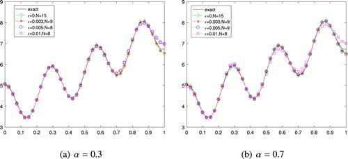
Example 6.1

Let $d=1,\mathrm{\Omega }=(0,1),T=1$. Take $m(t)=\cos (7\pi t)+e^t+2t+3$ and $n(x,t)\equiv 1$, $f(x,t)=\sin (\pi x)\sin (4\pi t)e^{-t}$. We take a numerical differentiation step size $\tau =0.01$. We choose the initial guess as $m^0=0.$ We set K = 11.

The numerical results for Example 6.1 with various noise levels $\epsilon =0,0.003,0.005,0.01$ in the case of $\alpha =0.3,0.7$ are shown in Figure 1. We can see that the numerical results for Example 1 match the exact ones quite well even up to $1\mathrm{\%}$ noise added in the exact data ${\int }_{\mathrm{\Omega }}{u}^2(x,t)\mathrm{d}x.$

Figure 1. The numerical results and the exact solution for Example 6.1. (a) $\alpha =0.3$. (b) $\alpha =0.7$.

In Table 1, we show the numerical errors $r{e}_k$ with different α and ϵ. It can be seen that the numerical results become a little worse when the relative noise levels increase and not sensitive to the fractional order α.

Table 1. The numerical relative errors $r{e}_j$ of Example 1 for different α and ϵ.

$\epsilon \setminus \alpha$	0.1	0.2	0.3	0.4	0.5	0.6	0.7	0.8	0.9
0	0.0050	0.0049	0.0049	0.0047	0.0046	0.0044	0.0042	0.0040	0.0038
0.003	0.0091	0.0085	0.0051	0.0052	0.0055	0.0059	0.0064	0.0069	0.0070
0.005	0.0094	0.0144	0.0156	0.0168	0.0068	0.0077	0.0088	0.0100	0.0102
0.01	0.0110	0.0153	0.0164	0.0175	0.0187	0.0201	0.0223	0.0272	0.0189

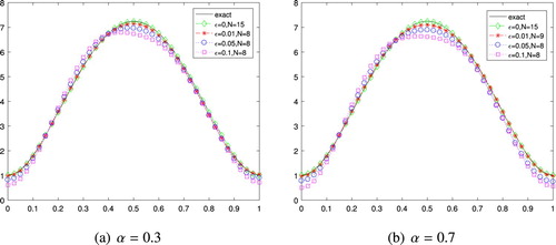
Example 6.2

Let $d=1,\mathrm{\Omega }=(0,1),T=1.$ Take $m(t)=100t^2(1-t{)}^2+1$ and $n(x,t)=1,f(x,t)=\sin (\pi x)\sin (4\pi t)e^{-t}$. We take a numerical differentiation step size $\tau =\mathrm{0.01.}$ We choose the initial guess as $m^0=0.$ We set K = 9.

The numerical results for Example 6.2 with various noise levels $\epsilon =0,0.01,0.05,0.1$ in the case of $\alpha =0.3,0.7$ are shown in Figure 2. We can see that the numerical results for Example 6.2 match the exact ones quite well even up to $10\mathrm{\%}$ noise added in the exact data ${\int }_{\mathrm{\Omega }}{u}^2(x,t)\mathrm{d}x.$

Figure 2. The numerical results and the exact solution for Example 6.2. (a) $\alpha =0.3$. (b) $\alpha =0.7$.

6.2. Two-dimensional case

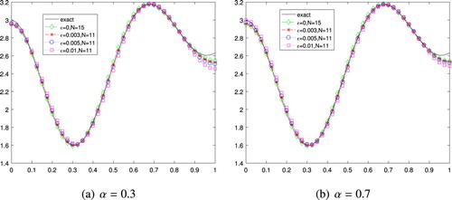
Example 6.3

Let $d=2,\mathrm{\Omega }=(0,1)\times (0,1),T=1$. Take $m(t)=e^{-t}\cos (3\pi t)+t+2$ and $n(x,y,t)=1,f(x,y,t)=\sin (\pi x)\sin (\pi y)\sin (2\pi t)e^{-t}$. We take a numerical differentiation step size $\tau =0.01$. We choose the initial guess as $m^0=0$. We set K = 5.

The numerical results for Example 6.3 with various noise levels $\epsilon =0,0.003,0.005,0.01$ in the case of $\alpha =0.3,0.7$ are shown in Figure 3. We can see that the numerical results for Example 6.3 match the exact ones quite well even up to $1\mathrm{\%}$ noise added in the exact data ${\int }_{\mathrm{\Omega }}{u}^2(x,y,t)\mathrm{d}x$.

Figure 3. The numerical results and the exact solution for Example 6.3 (a) $\alpha =0.3$. (b) $\alpha =0.7$.

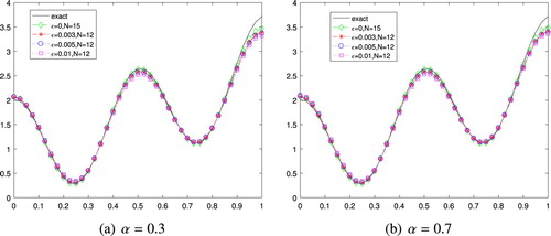
Example 6.4

Let $d=2,\mathrm{\Omega }=(0,1)\times (0,1),T=1.$ Take $m(t)=\cos (4\pi t)+e^t$ and $n(x,y,t)=1,f(x,y,t)=\sin (\pi x)\sin (\pi y)\sin (2\pi t)e^{-t}$. We take a numerical differentiation step size $\tau =0.01$. We choose the initial guess as $m^0=0$. We set K = 5.

The numerical results for Example 4 with various noise levels $\epsilon =0,0.003,0.005,0.01$ in the case of $\alpha =0.3,0.7$ are shown in Figure 4. We can see that the numerical results for Example 6.4 match the exact ones quite well even up to $1\mathrm{\%}$ noise added in the exact data ${\int }_{\mathrm{\Omega }}{u}^2(x,y,t)dx.$

Figure 4. The numerical results and the exact solution for Example 6.4. (a) $\alpha =0.3$. (b) $\alpha =0.7$.

7. Conclusions

In this paper, we investigate the time-dependent potential term in a time fractional diffusion equation. The existence, uniqueness and regularity of the solution for the direct problem are obtained by the fixed point theorem. Then the uniqueness of the solution for the inverse problem is provided by the property of Caputo fractional derivative. Finally, we employ the Levenberg–Marquardt method to find the approximation of the potential function.

Disclosure statement

No potential conflict of interest was reported by the author(s).

Additional information

Funding

This paper was supported by the National Natural Science Foundation of China (NSF of China) [11771192,11371181,11601216].

References

- Slodicka M, Van Keer R. Determination of a robin coefficient in semilinear parabolic problems by means of boundary measurements. Inverse Probl. 2002;18:139–152. doi: 10.1088/0266-5611/18/1/310
- Kubica A, Yamamoto M. Initial-booundary value problems for fractional diffusion equations with time-dependent coefficients. Fract Calc Appl Anal. 2018;21(2):276–311. doi: 10.1515/fca-2018-0018
- Li Z, Yamamoto M. Unique continuation principle for the one dimensional time fractional diffusion equation. Fract Calcul Appl Anal. 2019;22(3):644–657. doi: 10.1515/fca-2019-0036
- McLean W, Mustapha K, Ali R, et al. Well-posedness of time-fractional, advection-diffusion-reaction equations. Fract Calc Appl Anal. 2019;22(4):918–994. doi: 10.1515/fca-2019-0050
- Gorenflo R, Luchko R, Yamamoto M. Time fractional diffusion equation in the fractional Sobolev spaces. Fract Calc Appl Anal. 2015;18:799–820. doi: 10.1515/fca-2015-0048
- Liu Y, Rundell W, Yamamoto M. Strong maximum principle for fractional diffusion equations and an application to an inverse source problem. Fract Calc Appl Anal. 2016;19:888–906.
- Luchko Y. Maximum principle for the generalized time fractional diffusion equation. J Math Anal Appl. 2009;351:218–223. doi: 10.1016/j.jmaa.2008.10.018
- Sakamoto K, Yamamoto M. Initial value/boundary value problems for fractional diffusion-wave equations and applications to some inverse problems. J Math Anal Appl. 2011;382:426–447. doi: 10.1016/j.jmaa.2011.04.058
- Zhang Z. An undetermined time-dependent coefficient in a fractional diffusion equation. Inverse Probl Imaging. 2017;11(5):875–900. doi: 10.3934/ipi.2017041
- Zhang ZD. An undetermined coefficient problem for a fractional diffusion equation. Inverse Probl. 2016;32:015011.
- Fujishiro K, Kian Y. Determination of time dependent factors of coefficients in fractional diffusion equations. Math Control Relat Fields. 2016;6(2):251–269. doi: 10.3934/mcrf.2016003
- Sun LL, Zhang Y, Wei T. Recivering the time dependent potential function in a multi-term time fractional diffusion equation. Appl Numer Math. 2019;135:228–245. doi: 10.1016/j.apnum.2018.09.001
- Jin B, Rundell W. A tutorial on inverse problem for anomalous diffusion processes. Iverse Probl. 2015;31:035003.
- Jin BT, Rundell W. An inverse problem for a one-dimensional time-fractional diffusion problem. Inverse Probl. 2012;28:075010.
- Miller L, Yamamoto M. Coefficient inverse problem for a fractional diffusion equation. Inverse Probl. 2013;29(7):0750013. doi: 10.1088/0266-5611/29/7/075013
- Sun L, Wei T. Identification of zero order coefficient in a time fractional diffusion equation. Appl Numer Math. 2017;111:160–180. doi: 10.1016/j.apnum.2016.09.005
- Tuan VK. Inverse problem for fractional diffusion equation. Fract Calc Appl Anal. 2011;14(1):31–55. doi: 10.2478/s13540-011-0004-x
- Yamamoto M, Zhang Y. Conditional stability in determining a zeroth-order coefficient in a half-order fractional diffusion equation by a Carleman estimate. Inverse Probl. 2012;28(10):105010. doi: 10.1088/0266-5611/28/10/105010
- Zhang Z, Zhou Z. Recovering the potential term in a fractional diffusion equation. IMA J Appl Math. 2017;82:579–600. doi: 10.1093/imamat/hxx004
- Li Z, Yamamoto M. Inverse problems of determining coefficients of the fractional partial differential equations. In: Kochubei A, Luchko Y, editors, Handbook of fractional calculus with applications. Vol. 2; 2019. p. 443–464.
- Li Z, Yamamoto M. Inverse problems of determining sources of the fractional partial differential equations. Kochubei A, Luchko, Y, editors, Handbook of fractional calculus with applications. Vol. 2; 2019. p. 411–430.
- Liu Y, Li Z, Yamamoto M. Inverse problems of determining parameters of the fractional partial differential equations. Kochubei A, Luchko Y, editors, Handbook of fractional calculus with applications. Vol. 2; 2019. p. 431–442.
- Jiang D, Li Z, Liu Y, et al. Weak unique continuation and a related inverse source problem for time fractional diffusion equations. Inverse Probl. 2017;33(5):055013. doi: 10.1088/1361-6420/aa58d1
- Li Z, Imanuvilov OY, Yamamoto M. Uniqueness in inverse boundary value problems for fractional diffusion equations. Inverse Probl. 2016;32(1):015004. doi: 10.1088/0266-5611/32/1/015004
- Kilbas A, Srivastava H, Trujillo J. Theory and applications of fractional differential equations. Vol. 204. Amsterdam: Elsevier; 2006. 2453–2461.
- Alikhanov AA. Boundary value problems for the diffusion equation of the variable order in differential and difference settings. Appl Math Comput. 2012;219:3938–3946.
- Podlubny I. Fractional differential equations. San Diego: Acad Press. 1999.
- Brezis H. Functional analysis, sobolev spaces and partial differential equations. Universitext. 2012;88(2):117–126.
- Henry D. Geometric theory of semilinear parabolic equations. Berlin: Springer-Verlag; 1981. (Lecture Notes in Mathematics; 840).
- Pazy A. Semigroups of linear operators and applications to partial differential equations. Berlin,: Springer-Verlag; 1983.
- Fujiwara D. Concrete characterization of the domains of fractional powers of some elliptic differential operators of the second order. Proc Jpn Acad. 1967;43(2):82–86. doi: 10.3792/pja/1195521686
- Gorenflo R, Yamamoto M. Operator-theoretic treatment of linear abel integral equation of first kind. Jpn J Ind Appl Math. 1999;16(1):137–161. doi: 10.1007/BF03167528
- Courant R, Hilbert D. Methods of mathematical physics. Vol. 1, New York: Interscience; 1953.
- Royden HL. Real analysis. Vol. 71. Princeton: Princeton University Press; 1963. 402.
- Morozov V, Nashed Z, Aries A. Methods for solving incorrectly posed problems. New York: Springer-Verlag; 1984.
- Hanke M, Hansen P. Regularization methods for large-scale problems. Surv Math Ind. 1993;3(4):253–315.
- Murio DA. Implicit finite difference approximation for time fractional diffusion equations. Comput Math Appl. 2008;56(4):1138–1145. doi: 10.1016/j.camwa.2008.02.015