A spring-damping regularization of the Fourier sine series solution to the inverse Cauchy problem for a 3D sideways heat equation

Abstract

For solving the inverse Cauchy problem of a three-dimensional (3D) non-homogeneous sideways heat equation in a cuboid, we first transform it into a partial homogeneous boundary value problem, using a time-dependent two-dimensional (2D) homogenization technique. After a time step-by-step approach of the inverse Cauchy problem, it becomes an inverse Cauchy problem of the 3D modified Helmholtz equation. A sequence of 2D sine functions and a set of second-order ordinary differential equations are derived to determine the expansion coefficients, which can be solved in closed-form. In order to stably solve the inverse Cauchy problem, we simply introduce a spring-damping regularization technique to modify the coefficients, which results in a regularized 2D Fourier sine series solution of the unknown Dirichlet data on the top of the cuboid. The novel method can find the solution in the whole domain, which is quite accurate with small errors, even a large noise up to $20\mathrm{\%}$ is imposed on the given data. The present method together with the analyses of regularization parameter and the stability of solution is novel and shows promise in the 3D sideways problems of the heat equation.

Keywords:

• 3D sideways heat equation
• inverse Cauchy problem
• 2D homogenization function
• Fourier sine series solution
• spring-damping regularization

2010 Mathematics Subject Classifications:

• 35K55
• 35K05
• 65M32
• 68U20
• 35K15

1. Introduction

Let us consider a three-dimensional (3D) non-homogeneous and transient sideways heat equation (SHE): (1) $\begin{array}{rl}& \begin{array}{l}{u}_t(x,y,z,t)=u_{xx}(x,y,z,t)+u_{yy}(x,y,z,t)+u_{zz}(x,y,z,t)+S(x,y,z,t),\\ (x,y,z,t)\in \mathrm{\Omega }:=\{0<x<a,0<y<b,0<z<c,0<t\le t_f\},\end{array}\end{array}$(1) (2) $\begin{array}{rl}& u(x,y,z,0)=f(x,y,z),\end{array}$(2) (3) $\begin{array}{rl}& \begin{array}{l}u(0,y,z,t)=h_1(y,z,t),u(a,y,z,t)=h_2(y,z,t),u(x,0,z,t)=h_3(x,z,t),\\ u(x,b,z,t)=h_4(x,z,t),u(x,y,0,t)=h_5(x,y,t),u_z(x,y,0,t)=h_6(x,y,t),\end{array}\end{array}$(3) where the heat source and all the boundary conditions are time-dependent.

In Equations (1(1) $\begin{array}{rl}& \begin{array}{l}{u}_t(x,y,z,t)=u_{xx}(x,y,z,t)+u_{yy}(x,y,z,t)+u_{zz}(x,y,z,t)+S(x,y,z,t),\\ (x,y,z,t)\in \mathrm{\Omega }:=\{0<x<a,0<y<b,0<z<c,0<t\le t_f\},\end{array}\end{array}$(1) ) and (3(3) $\begin{array}{rl}& \begin{array}{l}u(0,y,z,t)=h_1(y,z,t),u(a,y,z,t)=h_2(y,z,t),u(x,0,z,t)=h_3(x,z,t),\\ u(x,b,z,t)=h_4(x,z,t),u(x,y,0,t)=h_5(x,y,t),u_z(x,y,0,t)=h_6(x,y,t),\end{array}\end{array}$(3) ), the data $u(x,y,c,t)$ are not specified on the top of the cuboid; however, we over-specify the Neumann data $u_z(x,y,0,t)=h_6(x,y,t)$ in order to recover $u(x,y,c,t)$, such that the total boundary data are completed. This is one sort of the inverse Cauchy problems in the cuboid for the 3D heat equation, which is usually named the sideways heat equation (SHE) in the literature. We must emphasize that the 3D SHE is more difficult than the inverse Cauchy problem of the 3D Poisson equation in a cuboid, i.e. the steady-state version of the 3D SHE.

Many researchers are interested in dealing with the SHE by utilizing mesh methods and meshless approaches. About the mesh algorithms, the finite difference discretizations for the SHE were discussed in [1]. Besides, the stability standpoints of those finite difference methods (FDMs) with mollification are contemplated in a series of papers; see, e.g. [2–6]. In those computations with the space-marching, FDMs are also delineated. Seidman and Eldén [7] proposed a filtering method (so-called the discrete Fourier transform) for calculating an approximate solution of the sideways heat equation. Then, Eldén [8,9] discretized the SHE by a differential-difference equation and explained the properties of time-discrete approximations by employing the Fourier transform methods. He revealed that the time discretization has a ‘regularizing effect,’ and the high-frequency noise is prevented from blowing up. Later, Regińska [10] addressed this ill-posed problem on the basis of an application of wavelet basis decomposition of measured data. The Meyer wavelets were applied to formulate a regularized solution, which was convergent to the exact one when the data error tended to zero. Regińska and Eldén [11] tackled the sideways problem numerically in the coarse level representation, as an ordinary differential equation in the space variable, where the time derivative was replaced by its wavelet representation. After that, Berntsson [12] claimed that the spectral scheme can eliminate much of the effect from the high-frequency noise in the measured data.

Subsequent to [12], Dorroh and Ru [13] used the method of quasi-reversibility and the FDM to compute the numerical solution of the SHE and showed that the numerical solution matched the exact solution well. Then, Eldén et al. [14] employed three methods for solving the SHE on the basis of approximating the time derivative by a bounded operator. Their approach can also be applied to the issues with variable coefficients; however, those results were not accurate. Regińska [15] utilized a certain simple nonlinear modification of the method based on local refinements of the wavelet expansion of the noisy data. Furthermore, he also presented that the accuracy of the solution reconstruction can be improved by adding some sufficiently large coefficients on the level higher than that indicated by the convergence theorem. Fu et al. [16] modified the results in [10] and provided a complete proof, from which a new interesting constant e${}^{\ast }$ is introduced. Then, Qiu et al. [17] proposed a new wavelet regularization method for the SHE and obtained a stable solution. Berntsson [18] demonstrated that his approach can solve the SHE in real time. Later, Wang [19] addressed the multi-resolution method based on the Shannon multi-resolution analysis to obtain a well-posed approximation and acquired an estimate for the difference between the exact solution and the solution of the approximating problem. Xiong et al. [20] used the Fourier regularization method together with the order optimal logarithmic stability estimates. Then, Wang [21] defined a wavelet solution to obtain the well-posed approximating problem in the scaling space and gave the proof of uniform convergence. Deng and Liu [22] introduced a new class of iteration methods to solve the SHE and proved that their methods were of order optimal under both a priori and a posteriori stopping rules. Pakanen [23] utilized the inverse procedure, which was based on a recursive deconvolution algorithm derived from the direct solution. Nguyen and Luu [24] employed the two new classes of quasi-type methods and iteration methods to solve the problem and proved that their schemes were stable under both a priori and a posteriori parameter choice rules. Those above-mentioned references did not mention the noise effect with their approaches.

Chang et al. [25] employed the group preserving scheme to tackle the SHE polluted by noises and acquired good results. Recently, Chang et al. [26] have reviewed the inverse heat conduction problems in detail. For the meshless scheme, Yu et al. [27] adopted the traditional Tikhonov regularization technique to tackle the ill-posedness of the SHE and obtained a stable solution to the system of ordinary differential equations.

Besides, only a few researchers propose a new scheme to tackle the 3D SHE. Before the construction of the two-dimensional (2D) Fourier sine series method to solve the 3D SHE, a key step is the construction of a time-dependent 2D homogenization function, such that the partial boundary conditions become zeros for the new variable. Previously, only the time-dependent one-dimensional homogenization functions are established [28,29], which were used to solve the inverse heat source problem of the one-dimensional heat equation. Then, Liu et al. [30] employed the 2D homogenization function technique in 1D space and time to recover the wave source.

The paper is arranged as follows. In Section 2, we construct a time-dependent 2D homogenization function. By using the Euler forward method, we transform the inverse Cauchy problem of 3D SHE into an inverse Cauchy problem of the 3D modified Helmholtz equation in Section 3. After a homogenization technique, we can express the new variable in terms of the 2D Fourier sine series as to be shown in Section 4, where a set of second-order ordinary differential equations (ODEs) are derived to determine the expansion coefficients in the 2D Fourier sine series. The closed-form solutions of the derived ODEs are obtained, which are however unstable. Thus, in Section 5 we introduce a simple spring-damping regularization technique to stabilize the unstable second-order ODEs. An example is given to select the regularization parameter. Then, we apply the spring-damping regularization technique to modify the expansion coefficients in the 2D Fourier sine series, which leads to a stable algorithm in Section 6 to solve the 3D sideways heat conduction problem in the whole cuboid, where the analysis of the stability of solution is given. While the regularization analysis and the numerical tests are given in Section 7, the conclusions are drawn in Section 8.

2. A time-dependent 2D homogenization function

In order to solve the 3D inverse Cauchy problem of the sideways heat equation by using the Fourier sine series method, the first key step is the construction of a time-dependent 2D homogenization function $B(x,y,z,t)$, such that the first four boundary conditions are zeros for the new variable: (4) $v(x,y,z,t)=u(x,y,z,t)-B(x,y,z,t).$(4) We first give a sequential construction technique of the homogenization function by starting from a time-independent 1D boundary value problem (BVP), which is easy $\begin{array}{rl}& \mathcal{L}\left[u\right(x\left)\right]=S\left(x\right),x\in (0,a),\\ & u\left(0\right)=u_0,u\left(a\right)=u_a,\end{array}$ where $\mathcal{L}$ is a linear differential operator.

From $B\left(x\right)=u_0\left(1-\frac{x}{a}\right)+\frac{x}{a}{u}_a,$ it readily follows that $B\left(0\right)=u_0,B\left(a\right)=u_a.$ Let $v\left(x\right)=u\left(x\right)-B\left(x\right).$ We have $\begin{array}{rl}& \mathcal{L}\left[v\right(x\left)\right]=S\left(x\right)-\mathcal{L}\left[B\right(x\left)\right],x\in (0,a),\\ & v\left(0\right)=0,v\left(a\right)=0.\end{array}$ Then, the 2D boundary value problem is slightly difficult $\begin{array}{rl}& \mathcal{L}\left[u\right(x,y\left)\right]=S(x,y),(x,y)\in (0,a)\times (0,b),\\ & u(0,y)=h_1\left(y\right),u(a,y)=h_2\left(y\right),\\ & u(x,0)=h_3\left(x\right),u(x,b)=h_4\left(x\right).\end{array}$ Upon letting $B^0(x,y)=h_1\left(y\right)\left(1-\frac{x}{a}\right)+\frac{x}{a}{h}_2\left(y\right),$ it follows that $B^0(0,y)=h_1\left(y\right),B^0(a,y)=h_2\left(y\right).$ Let $B(x,y)=B^0(x,y)+\left(1-\frac{y}{b}\right)\left[h_3\right(x)-B^0(x,0\left)\right]+\frac{y}{b}\left[h_4\right(x)-B^0(x,b\left)\right],$ and then we can check $\begin{array}{rl}& B(0,y)=h_1\left(y\right),B(a,y)=h_2\left(y\right),\\ & B(x,0)=h_3\left(x\right),B(x,b)=h_4\left(x\right),\end{array}$ where we have used the following compatibility conditions: $\begin{array}{rl}& h_3\left(0\right)=B^0(0,0)=h_1\left(0\right),\\ & h_4\left(0\right)=B^0(0,b)=h_1\left(b\right),\\ & h_3\left(a\right)=B^0(a,0)=h_2\left(0\right),\\ & h_4\left(a\right)=B^0(a,b)=h_2\left(b\right).\end{array}$ Therefore, we come to a 2D homogenization function for the 2D time-independent boundary value problem: (5) $\begin{array}{rl}B(x,y)& =\left(1-\frac{x}{a}\right)\left[h_1\left(y\right)-\left(1-\frac{y}{b}\right)h_3\left(0\right)-\frac{y}{b}{h}_4\left(0\right)\right]\\ & +\frac{x}{a}\left[h_2\left(y\right)-\left(1-\frac{y}{b}\right)h_3\left(a\right)-\frac{y}{b}{h}_4\left(a\right)\right]+\left(1-\frac{y}{b}\right)h_3\left(x\right)+\frac{y}{b}{h}_4\left(x\right).\end{array}$(5) In this course, we can transform the original 2D BVP with non-homogeneous boundary conditions to one with homogeneous boundary conditions: $\begin{array}{rl}& \mathcal{L}\left[v\right(x,y\left)\right]=S(x,y)-\mathcal{L}\left[B\right(x,y\left)\right],(x,y)\in (0,a)\times (0,b),\\ & v(0,y)=v(a,y)=v(x,0)=v(x,b)=0,\end{array}$ with the help of the variable transformation from $u(x,y)$ to $v(x,y)=u(x,y)-B(x,y)$. For its capability to annihilate all the non-zero boundary conditions in the BVP, $B(x,y)$ is called a 2D homogenization function.

As shown in Equation (3(3) $\begin{array}{rl}& \begin{array}{l}u(0,y,z,t)=h_1(y,z,t),u(a,y,z,t)=h_2(y,z,t),u(x,0,z,t)=h_3(x,z,t),\\ u(x,b,z,t)=h_4(x,z,t),u(x,y,0,t)=h_5(x,y,t),u_z(x,y,0,t)=h_6(x,y,t),\end{array}\end{array}$(3) ), the first four boundary conditions are functions of $(y,z,t)$ or $(x,z,t)$. Hence, replacing $h_1\left(y\right)$, $h_2\left(y\right)$, $h_3\left(x\right)$ and $h_4\left(x\right)$ in Equation (5(5) $\begin{array}{rl}B(x,y)& =\left(1-\frac{x}{a}\right)\left[h_1\left(y\right)-\left(1-\frac{y}{b}\right)h_3\left(0\right)-\frac{y}{b}{h}_4\left(0\right)\right]\\ & +\frac{x}{a}\left[h_2\left(y\right)-\left(1-\frac{y}{b}\right)h_3\left(a\right)-\frac{y}{b}{h}_4\left(a\right)\right]+\left(1-\frac{y}{b}\right)h_3\left(x\right)+\frac{y}{b}{h}_4\left(x\right).\end{array}$(5) ) by $h_1(y,z,t)$, $h_2(y,z,t)$, $h_3(x,z,t)$ and $h_4(x,z,t)$, we can produce the following partial 2D homogenization function: (6) $\begin{array}{rl}B(x,y,z,t)& =\left(1-\frac{x}{a}\right)\left[h_1(y,z,t)-\left(1-\frac{y}{b}\right)h_3(0,z,t)-\frac{y}{b}{h}_4(0,z,t)\right]\\ & +\frac{x}{a}\left[h_2(y,z,t)-\left(1-\frac{y}{b}\right)h_3(a,z,t)-\frac{y}{b}{h}_4(a,z,t)\right]\\ & +\left(1-\frac{y}{b}\right)h_3(x,z,t)+\frac{y}{b}{h}_4(x,z,t),\end{array}$(6) which satisfies the first four boundary conditions in Equation (3(3) $\begin{array}{rl}& \begin{array}{l}u(0,y,z,t)=h_1(y,z,t),u(a,y,z,t)=h_2(y,z,t),u(x,0,z,t)=h_3(x,z,t),\\ u(x,b,z,t)=h_4(x,z,t),u(x,y,0,t)=h_5(x,y,t),u_z(x,y,0,t)=h_6(x,y,t),\end{array}\end{array}$(3) ), i.e. (7) $\begin{array}{rl}& B(0,y,z,t)=h_1(y,z,t),B(a,y,z,t)=h_2(y,z,t),\\ & B(x,0,z,t)=h_3(x,z,t),B(x,b,z,t)=h_4(x,z,t),\end{array}$(7) where the consistent conditions $h_1(0,z,t)=h_3(0,z,t)$, $h_1(b,z,t)=h_4(0,z,t)$, $h_2(0,z,t)=h_3(a,z,t)$ and $h_2(b,z,t)=h_4(a,z,t)$ were used.

Further development of the homogenization functions to different types and used them as mathematical tools to solve other engineering inverse and direct problems were carried out in [31–36].

3. A time step-by-step approach

Let $\overline{\mathrm{\Omega }}:=\mathrm{\Omega }\cup \mathrm{\Gamma }$, where Γ is the boundary of Ω. We suppose that (8) $\begin{array}{rl}& |S(x,y,z,t)|\le S_0,(x,y,z,t)\in \overline{\mathrm{\Omega }},\end{array}$(8) (9) $\begin{array}{rl}& h_i\in {\mathcal{C}}^2\left(\overline{\mathrm{\Omega }}\right)\Rightarrow |h_i|\le h_i^0,(x,y,z,t)\in \overline{\mathrm{\Omega }},i=1,\dots ,6,\end{array}$(9) where $S_0$ and $h_i^0$ are some constants. We suppose that (10) $|f(x,y,z)|\le f_0$(10) is a bounded function and $f_0$ is a constant. A direct result of Equations (6(6) $\begin{array}{rl}B(x,y,z,t)& =\left(1-\frac{x}{a}\right)\left[h_1(y,z,t)-\left(1-\frac{y}{b}\right)h_3(0,z,t)-\frac{y}{b}{h}_4(0,z,t)\right]\\ & +\frac{x}{a}\left[h_2(y,z,t)-\left(1-\frac{y}{b}\right)h_3(a,z,t)-\frac{y}{b}{h}_4(a,z,t)\right]\\ & +\left(1-\frac{y}{b}\right)h_3(x,z,t)+\frac{y}{b}{h}_4(x,z,t),\end{array}$(6) ) and (9(9) $\begin{array}{rl}& h_i\in {\mathcal{C}}^2\left(\overline{\mathrm{\Omega }}\right)\Rightarrow |h_i|\le h_i^0,(x,y,z,t)\in \overline{\mathrm{\Omega }},i=1,\dots ,6,\end{array}$(9) ) is that (11) $B(x,y,z,t)\in {\mathcal{C}}^2\left(\overline{\mathrm{\Omega }}\right)\Rightarrow |B(x,y,z,t)|\le B_0,(x,y,z,t)\in \overline{\mathrm{\Omega }},$(11) where $B_0$ is a constant. With those regularity assumptions, we are going to solve the 3D SHE in Equations (1(1) $\begin{array}{rl}& \begin{array}{l}{u}_t(x,y,z,t)=u_{xx}(x,y,z,t)+u_{yy}(x,y,z,t)+u_{zz}(x,y,z,t)+S(x,y,z,t),\\ (x,y,z,t)\in \mathrm{\Omega }:=\{0<x<a,0<y<b,0<z<c,0<t\le t_f\},\end{array}\end{array}$(1) )–(3(3) $\begin{array}{rl}& \begin{array}{l}u(0,y,z,t)=h_1(y,z,t),u(a,y,z,t)=h_2(y,z,t),u(x,0,z,t)=h_3(x,z,t),\\ u(x,b,z,t)=h_4(x,z,t),u(x,y,0,t)=h_5(x,y,t),u_z(x,y,0,t)=h_6(x,y,t),\end{array}\end{array}$(3) ).

We approach the 3D inverse Cauchy problem (1(1) $\begin{array}{rl}& \begin{array}{l}{u}_t(x,y,z,t)=u_{xx}(x,y,z,t)+u_{yy}(x,y,z,t)+u_{zz}(x,y,z,t)+S(x,y,z,t),\\ (x,y,z,t)\in \mathrm{\Omega }:=\{0<x<a,0<y<b,0<z<c,0<t\le t_f\},\end{array}\end{array}$(1) )–(3(3) $\begin{array}{rl}& \begin{array}{l}u(0,y,z,t)=h_1(y,z,t),u(a,y,z,t)=h_2(y,z,t),u(x,0,z,t)=h_3(x,z,t),\\ u(x,b,z,t)=h_4(x,z,t),u(x,y,0,t)=h_5(x,y,t),u_z(x,y,0,t)=h_6(x,y,t),\end{array}\end{array}$(3) ) of the SHE by a time step-by-step method, which supposes that $u(x,y,z,t)$ is solved in the previous time step. Initially, we can take $u(x,y,z,0)=f(x,y,z)$. Thus, we may approximate Equation (1(1) $\begin{array}{rl}& \begin{array}{l}{u}_t(x,y,z,t)=u_{xx}(x,y,z,t)+u_{yy}(x,y,z,t)+u_{zz}(x,y,z,t)+S(x,y,z,t),\\ (x,y,z,t)\in \mathrm{\Omega }:=\{0<x<a,0<y<b,0<z<c,0<t\le t_f\},\end{array}\end{array}$(1) ) by using the Euler forward method (12) $\begin{array}{rl}& u_{xx}(x,y,z,t+\mathrm{\Delta }t)+u_{yy}(x,y,z,t+\mathrm{\Delta }t)+u_{zz}(x,y,z,t+\mathrm{\Delta }t)\\ & =\lambda u(x,y,z,t+\mathrm{\Delta }t)-\lambda u(x,y,z,t)-S(x,y,z,t+\mathrm{\Delta }t),\end{array}$(12) where $\mathrm{\Delta }t$ is a time increment and $\lambda =1/\mathrm{\Delta }t$. Equation (12(12) $\begin{array}{rl}& u_{xx}(x,y,z,t+\mathrm{\Delta }t)+u_{yy}(x,y,z,t+\mathrm{\Delta }t)+u_{zz}(x,y,z,t+\mathrm{\Delta }t)\\ & =\lambda u(x,y,z,t+\mathrm{\Delta }t)-\lambda u(x,y,z,t)-S(x,y,z,t+\mathrm{\Delta }t),\end{array}$(12) ) together with the boundary conditions in Equation (3(3) $\begin{array}{rl}& \begin{array}{l}u(0,y,z,t)=h_1(y,z,t),u(a,y,z,t)=h_2(y,z,t),u(x,0,z,t)=h_3(x,z,t),\\ u(x,b,z,t)=h_4(x,z,t),u(x,y,0,t)=h_5(x,y,t),u_z(x,y,0,t)=h_6(x,y,t),\end{array}\end{array}$(3) ) constitute an inverse Cauchy problem for the modified Helmholtz equation to solve $u(x,y,z,t+\mathrm{\Delta }t)$.

For simplicity, we do not employ the Crank–Nicolson and the Runge–Kutta integration methods to approach Equation (1(1) $\begin{array}{rl}& \begin{array}{l}{u}_t(x,y,z,t)=u_{xx}(x,y,z,t)+u_{yy}(x,y,z,t)+u_{zz}(x,y,z,t)+S(x,y,z,t),\\ (x,y,z,t)\in \mathrm{\Omega }:=\{0<x<a,0<y<b,0<z<c,0<t\le t_f\},\end{array}\end{array}$(1) ) in the time-direction; otherwise, Equation (12(12) $\begin{array}{rl}& u_{xx}(x,y,z,t+\mathrm{\Delta }t)+u_{yy}(x,y,z,t+\mathrm{\Delta }t)+u_{zz}(x,y,z,t+\mathrm{\Delta }t)\\ & =\lambda u(x,y,z,t+\mathrm{\Delta }t)-\lambda u(x,y,z,t)-S(x,y,z,t+\mathrm{\Delta }t),\end{array}$(12) ) would become very complex, which is no more an inverse Cauchy problem for the modified Helmholtz equation.

Now, let us introduce the following variable transformation from $u(x,y,z,t+\mathrm{\Delta }t)$ to $v(x,y,z,t+\mathrm{\Delta }t)$ by (13) $v(x,y,z,t+\mathrm{\Delta }t)=u(x,y,z,t+\mathrm{\Delta }t)-B(x,y,z,t+\mathrm{\Delta }t).$(13) Then inserting Equation (13(13) $v(x,y,z,t+\mathrm{\Delta }t)=u(x,y,z,t+\mathrm{\Delta }t)-B(x,y,z,t+\mathrm{\Delta }t).$(13) ) for $u(x,y,z,t+\mathrm{\Delta }t)=v(x,y,z,t+\mathrm{\Delta }t)+B(x,y,z,t+\mathrm{\Delta }t)$ into Equation (12(12) $\begin{array}{rl}& u_{xx}(x,y,z,t+\mathrm{\Delta }t)+u_{yy}(x,y,z,t+\mathrm{\Delta }t)+u_{zz}(x,y,z,t+\mathrm{\Delta }t)\\ & =\lambda u(x,y,z,t+\mathrm{\Delta }t)-\lambda u(x,y,z,t)-S(x,y,z,t+\mathrm{\Delta }t),\end{array}$(12) ), we can obtain a new modified Helmholtz equation for $v(x,y,z,t+\mathrm{\Delta }t)$, which is equipped with the partial homogeneous boundary conditions (14) $\begin{array}{rl}& v_{xx}(x,y,z,t+\mathrm{\Delta }t)+v_{yy}(x,y,z,t+\mathrm{\Delta }t)+v_{zz}(x,y,z,t+\mathrm{\Delta }t)\\ & =\lambda v(x,y,z,t+\mathrm{\Delta }t)+F(x,y,z,t+\mathrm{\Delta }t),\end{array}$(14) (15) $\begin{array}{rl}& \begin{array}{l}v(0,y,z,t+\mathrm{\Delta }t)=0,v(a,y,z,t+\mathrm{\Delta }t)=0,\\ v(x,0,z,t+\mathrm{\Delta }t)=0,v(x,b,z,t+\mathrm{\Delta }t)=0,\end{array}\end{array}$(15) and the two non-zero conditions at z = 0: (16) $\begin{array}{rl}v(x,y,0,t+\mathrm{\Delta }t)& =h_5(x,y,t+\mathrm{\Delta }t)-B(x,y,0,t+\mathrm{\Delta }t),\end{array}$(16) (17) $\begin{array}{rl}{v}_z(x,y,0,t+\mathrm{\Delta }t)& =h_6(x,y,t+\mathrm{\Delta }t)-B_z(x,y,0,t+\mathrm{\Delta }t),\end{array}$(17) where (18) $\begin{array}{rl}F(x,y,z,t+\mathrm{\Delta }t)& =\lambda B(x,y,z,t+\mathrm{\Delta }t)-S(x,y,z,t+\mathrm{\Delta }t)-\lambda u(x,y,z,t)\\ & -B_{xx}(x,y,z,t+\mathrm{\Delta }t)-B_{yy}(x,y,z,t+\mathrm{\Delta }t)-B_{zz}(x,y,z,t+\mathrm{\Delta }t).\end{array}$(18)

Remark 3.1

We give some comments about the homogenization function $B(x,y,z,t)$ in Equation (6(6) $\begin{array}{rl}B(x,y,z,t)& =\left(1-\frac{x}{a}\right)\left[h_1(y,z,t)-\left(1-\frac{y}{b}\right)h_3(0,z,t)-\frac{y}{b}{h}_4(0,z,t)\right]\\ & +\frac{x}{a}\left[h_2(y,z,t)-\left(1-\frac{y}{b}\right)h_3(a,z,t)-\frac{y}{b}{h}_4(a,z,t)\right]\\ & +\left(1-\frac{y}{b}\right)h_3(x,z,t)+\frac{y}{b}{h}_4(x,z,t),\end{array}$(6) ), of which $s_1\left(x\right)=1-x/a$, $s_2\left(x\right)=x/a$, $s_3\left(y\right)=1-y/b$, $s_4\left(y\right)=y/b$ are named shape functions (or interpolation functions). The basic requirements of these functions are (19) $\begin{array}{rl}& s_1\left(0\right)=1,s_1\left(a\right)=0,s_2\left(0\right)=0,s_2\left(a\right)=1,\end{array}$(19) (20) $\begin{array}{rl}& s_3\left(0\right)=1,s_3\left(b\right)=0,s_4\left(0\right)=0,s_4\left(b\right)=1.\end{array}$(20) There are many different ways to construct the shape functions, for example, the exponential functions (21) $\begin{array}{rl}& s_1\left(x\right)=\frac{e^a-e^x}{e^a-1},s_2\left(x\right)=\frac{e^x-1}{e^a-1},\end{array}$(21) (22) $\begin{array}{rl}& s_3\left(y\right)=\frac{e^b-e^y}{e^b-1},s_4\left(y\right)=\frac{e^y-1}{e^b-1}.\end{array}$(22) It is easily to check that these functions satisfy Equations (19(19) $\begin{array}{rl}& s_1\left(0\right)=1,s_1\left(a\right)=0,s_2\left(0\right)=0,s_2\left(a\right)=1,\end{array}$(19) ) and (20(20) $\begin{array}{rl}& s_3\left(0\right)=1,s_3\left(b\right)=0,s_4\left(0\right)=0,s_4\left(b\right)=1.\end{array}$(20) ). Therefore, if we replace $1-x/a$, x/a, $1-y/b$, y/b in $B(x,y,z,t)$ in Equation (6(6) $\begin{array}{rl}B(x,y,z,t)& =\left(1-\frac{x}{a}\right)\left[h_1(y,z,t)-\left(1-\frac{y}{b}\right)h_3(0,z,t)-\frac{y}{b}{h}_4(0,z,t)\right]\\ & +\frac{x}{a}\left[h_2(y,z,t)-\left(1-\frac{y}{b}\right)h_3(a,z,t)-\frac{y}{b}{h}_4(a,z,t)\right]\\ & +\left(1-\frac{y}{b}\right)h_3(x,z,t)+\frac{y}{b}{h}_4(x,z,t),\end{array}$(6) ) by the above $s_1\left(x\right)$, $s_2\left(x\right)$, $s_3\left(y\right)$, $s_4\left(y\right)$, we can construct another homogenization function $B(x,y,z,t)$. The homogenization function $B(x,y,z,t)$ is not unique.

However, the homogenization function $B(x,y,z,t)$ in Equation (6(6) $\begin{array}{rl}B(x,y,z,t)& =\left(1-\frac{x}{a}\right)\left[h_1(y,z,t)-\left(1-\frac{y}{b}\right)h_3(0,z,t)-\frac{y}{b}{h}_4(0,z,t)\right]\\ & +\frac{x}{a}\left[h_2(y,z,t)-\left(1-\frac{y}{b}\right)h_3(a,z,t)-\frac{y}{b}{h}_4(a,z,t)\right]\\ & +\left(1-\frac{y}{b}\right)h_3(x,z,t)+\frac{y}{b}{h}_4(x,z,t),\end{array}$(6) ) is the simplest one, which greatly simplifies the terms $B_{xx}(x,y,z,t+\mathrm{\Delta }t)$ and $B_{yy}(x,y,z,t+\mathrm{\Delta }t)$ appeared in $F(x,y,z,t+\mathrm{\Delta }t)$ of Equation (18(18) $\begin{array}{rl}F(x,y,z,t+\mathrm{\Delta }t)& =\lambda B(x,y,z,t+\mathrm{\Delta }t)-S(x,y,z,t+\mathrm{\Delta }t)-\lambda u(x,y,z,t)\\ & -B_{xx}(x,y,z,t+\mathrm{\Delta }t)-B_{yy}(x,y,z,t+\mathrm{\Delta }t)-B_{zz}(x,y,z,t+\mathrm{\Delta }t).\end{array}$(18) ). If we employ the exponential functions in Equations (21(21) $\begin{array}{rl}& s_1\left(x\right)=\frac{e^a-e^x}{e^a-1},s_2\left(x\right)=\frac{e^x-1}{e^a-1},\end{array}$(21) ) and (22(22) $\begin{array}{rl}& s_3\left(y\right)=\frac{e^b-e^y}{e^b-1},s_4\left(y\right)=\frac{e^y-1}{e^b-1}.\end{array}$(22) ) as the shape functions, the calculation of $F(x,y,z,t+\mathrm{\Delta }t)$ would become tedious.

4. A 2D Fourier sine series method

By using the method of separation of variables, it follows that (23) $v(x,y,z,t+\mathrm{\Delta }t)=\sum _{i=1}^{\mathrm{\infty }}\sum _{j=1}^{\mathrm{\infty }}{T}_{ij}\left(z\right)\sin \frac{i\pi x}{a}\sin \frac{j\pi y}{b},$(23) which automatically satisfies the partial homogeneous boundary conditions in Equation (15(15) $\begin{array}{rl}& \begin{array}{l}v(0,y,z,t+\mathrm{\Delta }t)=0,v(a,y,z,t+\mathrm{\Delta }t)=0,\\ v(x,0,z,t+\mathrm{\Delta }t)=0,v(x,b,z,t+\mathrm{\Delta }t)=0,\end{array}\end{array}$(15) ). If we can solve $T_{ij}\left(z\right),$ then the analytic solution of $v(x,y,z,t+\mathrm{\Delta }t)$ is obtained in a form of the 2D Fourier sine series.

Multiplying both the sides of Equation (23(23) $v(x,y,z,t+\mathrm{\Delta }t)=\sum _{i=1}^{\mathrm{\infty }}\sum _{j=1}^{\mathrm{\infty }}{T}_{ij}\left(z\right)\sin \frac{i\pi x}{a}\sin \frac{j\pi y}{b},$(23) ) by $\sin \left(m\pi x/a\right)\sin \left(n\pi y/b\right)$, integrating it from x = 0 to x = a and y = 0 to y = b, and using the orthogonality of sinusoidal functions, we can formally write (24) $T_{ij}\left(z\right)=\frac{4}{ab}{\int }_0^b{\int }_0^{a}v(\xi ,\zeta ,z,t+\mathrm{\Delta }t)\sin \frac{i\pi \xi }{a}\sin \frac{j\pi \zeta }{b}\mathrm{d}\xi \mathrm{d}\zeta .$(24) Taking the z-differential of Equation (24(24) $T_{ij}\left(z\right)=\frac{4}{ab}{\int }_0^b{\int }_0^{a}v(\xi ,\zeta ,z,t+\mathrm{\Delta }t)\sin \frac{i\pi \xi }{a}\sin \frac{j\pi \zeta }{b}\mathrm{d}\xi \mathrm{d}\zeta .$(24) ) twice, we have (25) $T_{ij}^{″}\left(z\right)=\frac{4}{ab}{\int }_0^b{\int }_0^a{v}_{zz}(\xi ,\zeta ,z,t+\mathrm{\Delta }t)\sin \frac{i\pi \xi }{a}\sin \frac{j\pi \zeta }{b}\mathrm{d}\xi \mathrm{d}\zeta ,$(25) due to Equation (14(14) $\begin{array}{rl}& v_{xx}(x,y,z,t+\mathrm{\Delta }t)+v_{yy}(x,y,z,t+\mathrm{\Delta }t)+v_{zz}(x,y,z,t+\mathrm{\Delta }t)\\ & =\lambda v(x,y,z,t+\mathrm{\Delta }t)+F(x,y,z,t+\mathrm{\Delta }t),\end{array}$(14) ), which becomes (26) $\begin{array}{rl}{T}_{ij}^{″}\left(z\right)& =\frac{4}{ab}{\int }_0^b{\int }_0^{a}F(\xi ,\zeta ,z,t+\mathrm{\Delta }t)\sin \frac{i\pi \xi }{a}\sin \frac{j\pi \zeta }{b}\mathrm{d}\xi \mathrm{d}\zeta \\ & -\frac{4}{ab}{\int }_0^b{\int }_0^a\left[v_{\xi \xi }\right(\xi ,\zeta ,z,t+\mathrm{\Delta }t)+v_{\zeta \zeta }(\xi ,\zeta ,z,t+\mathrm{\Delta }t)\\ & -\lambda v(\xi ,\zeta ,z,t+\mathrm{\Delta }t)]\sin \frac{i\pi \xi }{a}\sin \frac{j\pi \zeta }{b}\mathrm{d}\xi \mathrm{d}\zeta .\end{array}$(26) Applying the integration by parts twice to the first two integral terms in the last two lines of Equation (26(26) $\begin{array}{rl}{T}_{ij}^{″}\left(z\right)& =\frac{4}{ab}{\int }_0^b{\int }_0^{a}F(\xi ,\zeta ,z,t+\mathrm{\Delta }t)\sin \frac{i\pi \xi }{a}\sin \frac{j\pi \zeta }{b}\mathrm{d}\xi \mathrm{d}\zeta \\ & -\frac{4}{ab}{\int }_0^b{\int }_0^a\left[v_{\xi \xi }\right(\xi ,\zeta ,z,t+\mathrm{\Delta }t)+v_{\zeta \zeta }(\xi ,\zeta ,z,t+\mathrm{\Delta }t)\\ & -\lambda v(\xi ,\zeta ,z,t+\mathrm{\Delta }t)]\sin \frac{i\pi \xi }{a}\sin \frac{j\pi \zeta }{b}\mathrm{d}\xi \mathrm{d}\zeta .\end{array}$(26) ), and using the boundary conditions (15(15) $\begin{array}{rl}& \begin{array}{l}v(0,y,z,t+\mathrm{\Delta }t)=0,v(a,y,z,t+\mathrm{\Delta }t)=0,\\ v(x,0,z,t+\mathrm{\Delta }t)=0,v(x,b,z,t+\mathrm{\Delta }t)=0,\end{array}\end{array}$(15) ) and Equation (24(24) $T_{ij}\left(z\right)=\frac{4}{ab}{\int }_0^b{\int }_0^{a}v(\xi ,\zeta ,z,t+\mathrm{\Delta }t)\sin \frac{i\pi \xi }{a}\sin \frac{j\pi \zeta }{b}\mathrm{d}\xi \mathrm{d}\zeta .$(24) ), we can derive a set of second-order ordinary differential equations (ODEs) for the expansion coefficients $T_{ij}\left(z\right)$: (27) $T_{ij}^{″}\left(z\right)=({\mu }_{ij}+\lambda )T_{ij}\left(z\right)+F_{ij}(z,t+\mathrm{\Delta }t),$(27) where (28) $\begin{array}{rl}& {\mu }_{ij}:={\left(\frac{i\pi }{a}\right)}^2+{\left(\frac{j\pi }{b}\right)}^2,\end{array}$(28) (29) $\begin{array}{rl}& F_{ij}(z,t+\mathrm{\Delta }t):=\frac{4}{ab}{\int }_0^b{\int }_0^{a}F(\xi ,\zeta ,z,t+\mathrm{\Delta }t)\sin \frac{i\pi \xi }{a}\sin \frac{j\pi \zeta }{b}\mathrm{d}\xi \mathrm{d}\zeta .\end{array}$(29) The corresponding initial conditions in the z-direction are available from Equations (24(24) $T_{ij}\left(z\right)=\frac{4}{ab}{\int }_0^b{\int }_0^{a}v(\xi ,\zeta ,z,t+\mathrm{\Delta }t)\sin \frac{i\pi \xi }{a}\sin \frac{j\pi \zeta }{b}\mathrm{d}\xi \mathrm{d}\zeta .$(24) ), (16(16) $\begin{array}{rl}v(x,y,0,t+\mathrm{\Delta }t)& =h_5(x,y,t+\mathrm{\Delta }t)-B(x,y,0,t+\mathrm{\Delta }t),\end{array}$(16) ) and (17(17) $\begin{array}{rl}{v}_z(x,y,0,t+\mathrm{\Delta }t)& =h_6(x,y,t+\mathrm{\Delta }t)-B_z(x,y,0,t+\mathrm{\Delta }t),\end{array}$(17) ) (30) $\begin{array}{rl}& T_{ij}\left(0\right)=\frac{4}{ab}{\int }_0^b{\int }_0^a\left[h_5\right(\xi ,\zeta ,t+\mathrm{\Delta }t)-B(\xi ,\zeta ,0,t+\mathrm{\Delta }t\left)\right]\sin \frac{i\pi \xi }{a}\sin \frac{j\pi \zeta }{b}\mathrm{d}\xi \mathrm{d}\zeta ,\end{array}$(30) (31) $\begin{array}{rl}& T_{ij}^{\prime }\left(0\right)=\frac{4}{ab}{\int }_0^b{\int }_0^a\left[h_6\right(\xi ,\zeta ,t+\mathrm{\Delta }t)-B_z(\xi ,\zeta ,0,t+\mathrm{\Delta }t\left)\right]\sin \frac{i\pi \xi }{a}\sin \frac{j\pi \zeta }{b}\mathrm{d}\xi \mathrm{d}\zeta .\end{array}$(31) Because the functions F, B, $h_5$ and $h_6$ are assumed to be smooth enough, there exist no Gibbs phenomena. With the regularity assumptions (9(9) $\begin{array}{rl}& h_i\in {\mathcal{C}}^2\left(\overline{\mathrm{\Omega }}\right)\Rightarrow |h_i|\le h_i^0,(x,y,z,t)\in \overline{\mathrm{\Omega }},i=1,\dots ,6,\end{array}$(9) ) and (11(11) $B(x,y,z,t)\in {\mathcal{C}}^2\left(\overline{\mathrm{\Omega }}\right)\Rightarrow |B(x,y,z,t)|\le B_0,(x,y,z,t)\in \overline{\mathrm{\Omega }},$(11) ), we have (32) $|T_{ij}\left(0\right)|\le C_1,|T_{ij}^{\prime }\left(0\right)|\le C_2,$(32) where $C_1$ and $C_2$ are constants.

Unfortunately, the coefficient ${\mu }_{ij}+\lambda$ in Equation (27(27) $T_{ij}^{″}\left(z\right)=({\mu }_{ij}+\lambda )T_{ij}\left(z\right)+F_{ij}(z,t+\mathrm{\Delta }t),$(27) ) is positive, i.e. ${\mu }_{ij}+\lambda >0$, which will cause the solution $T_{ij}\left(z\right)$ to blow up very fast. Without help from the regularization technique, it is hopeless to use $T_{ij}\left(z\right)$ as a solution medium to solve the inverse Cauchy problem of the 3D SHEs. Below, we will develop a regularization technique to stabilize the unstable ODEs.

5. A motivation of spring-damping regularization

Let us consider an initial value problem of a second-order ODE (33) $w^{″}\left(t\right)={\mu }^{2}w\left(t\right),$(33) where $\mu >0$. Because ${\mu }^{2}w\left(t\right)$ appears on the right-hand side, it is a spring term with a negative spring constant $-{\mu }^2<0$.

The general solution is unstable (34) $w\left(t\right)=c_1{e}^{\mu t}+c_2{e}^{-\mu t},$(34) where $c_1$ and $c_2$ are integration constants.

To stabilize the solution we may consider (35) $w\left(t\right)=c_{1}z\left(t\right)+c_2{e}^{-\mu t}=c_1\frac{1}{e^{-\mu t}+\alpha }+c_2{e}^{-\mu t},$(35) where $\alpha \ge 0$ is a regularization parameter, and when $\alpha =0$, Equation (35(35) $w\left(t\right)=c_{1}z\left(t\right)+c_2{e}^{-\mu t}=c_1\frac{1}{e^{-\mu t}+\alpha }+c_2{e}^{-\mu t},$(35) ) reduces to Equation (34(34) $w\left(t\right)=c_1{e}^{\mu t}+c_2{e}^{-\mu t},$(34) ).

Next, we want to derive the governing ODE for $w\left(t\right)$ in Equation (35(35) $w\left(t\right)=c_{1}z\left(t\right)+c_2{e}^{-\mu t}=c_1\frac{1}{e^{-\mu t}+\alpha }+c_2{e}^{-\mu t},$(35) ). Taking the time differentials of $w\left(t\right)$ in Equation (35(35) $w\left(t\right)=c_{1}z\left(t\right)+c_2{e}^{-\mu t}=c_1\frac{1}{e^{-\mu t}+\alpha }+c_2{e}^{-\mu t},$(35) ), we have (36) $\begin{array}{rl}{w}^{\prime }\left(t\right)& =c_1{z}^{\prime }\left(t\right)-\mu c_2{e}^{-\mu t},\end{array}$(36) (37) $\begin{array}{rl}{w}^{″}\left(t\right)& =c_1{z}^{″}\left(t\right)+{\mu }^2{c}_2{e}^{-\mu t}.\end{array}$(37) By cancelling $c_1$ and $c_2$ in Equations (35(35) $w\left(t\right)=c_{1}z\left(t\right)+c_2{e}^{-\mu t}=c_1\frac{1}{e^{-\mu t}+\alpha }+c_2{e}^{-\mu t},$(35) )–(37(37) $\begin{array}{rl}{w}^{″}\left(t\right)& =c_1{z}^{″}\left(t\right)+{\mu }^2{c}_2{e}^{-\mu t}.\end{array}$(37) ) it follows that (38) $w^{″}\left(t\right)={\mu }^{2}w\left(t\right)+\left[w^{\prime }\right(t)+\mu w(t\left)\right]\frac{z^{″}\left(t\right)-{\mu }^{2}z\left(t\right)}{z^{\prime }\left(t\right)+\mu z\left(t\right)},$(38) which, after inserting $z\left(t\right)=1/(e^{-\mu t}+\alpha )$ and its differentials, can be refined to (39) $w^{″}\left(t\right)+\alpha \mu \frac{\alpha +3e^{-\mu t}}{(\alpha +e^{-\mu t})(\alpha +2e^{-\mu t})}\left[w^{\prime }\right(t)+\mu w(t\left)\right]={\mu }^{2}w\left(t\right).$(39) Upon comparing with the unstable ODE in Equation (33(33) $w^{″}\left(t\right)={\mu }^{2}w\left(t\right),$(33) ), the stabilized ODE above possesses two extra terms in the left-hand side (40) $\begin{array}{rl}& \text{damping term}:\alpha \mu \frac{\alpha +3e^{-\mu t}}{(\alpha +e^{-\mu t})(\alpha +2e^{-\mu t})}{w}^{\prime }\left(t\right),\end{array}$(40) (41) $\begin{array}{rl}& \text{spring term}:\alpha {\mu }^2\frac{\alpha +3e^{-\mu t}}{(\alpha +e^{-\mu t})(\alpha +2e^{-\mu t})}w\left(t\right).\end{array}$(41) Therefore, the current regularization technique is one of the spring-damping regularizations [37,38]. The ODE in Equation (39(39) $w^{″}\left(t\right)+\alpha \mu \frac{\alpha +3e^{-\mu t}}{(\alpha +e^{-\mu t})(\alpha +2e^{-\mu t})}\left[w^{\prime }\right(t)+\mu w(t\left)\right]={\mu }^{2}w\left(t\right).$(39) ) brings the unstable solution $e^{\mu t}$ to a stable one $1/(e^{-\mu t}+\alpha )$, and meanwhile keeps the same stable solution $e^{-\mu t}$ unchanged.

When Equation (35(35) $w\left(t\right)=c_{1}z\left(t\right)+c_2{e}^{-\mu t}=c_1\frac{1}{e^{-\mu t}+\alpha }+c_2{e}^{-\mu t},$(35) ) is subjected to the initial conditions (42) $w\left(0\right)=a_0+s,w^{\prime }\left(0\right)=b_0+s,$(42) where s is a random noise, we can solve $c_1$ and $c_2$ and then the solution is given by (43) $\begin{array}{rl}{w}_r\left(t\right)& =\frac{(1+\alpha {)}^2}{\mu (2+\alpha )}[\mu a_0+b_0+(\mu +1\left)s\right]\frac{1}{e^{-\mu t}+\alpha }\\ & +\frac{1}{\mu (2+\alpha )}[\mu a_0-(1+\alpha )b_0+\mu s-(1+\alpha \left)s\right]e^{-\mu t},\end{array}$(43) where the subscript r denotes that $w_r$ is a regularized solution.

Let $t_f$ be a terminal time for the system of ODEs. In Equation (43(43) $\begin{array}{rl}{w}_r\left(t\right)& =\frac{(1+\alpha {)}^2}{\mu (2+\alpha )}[\mu a_0+b_0+(\mu +1\left)s\right]\frac{1}{e^{-\mu t}+\alpha }\\ & +\frac{1}{\mu (2+\alpha )}[\mu a_0-(1+\alpha )b_0+\mu s-(1+\alpha \left)s\right]e^{-\mu t},\end{array}$(43) ), we can observe that the error s is amplified by the factor $1/[e^{-\mu t}+\alpha ]$, and we ask that the solution error at $t=t_f$ is in the same level of the noise by (44) $\frac{s}{e^{-\mu t_f}+\alpha }=A_{0}s,$(44) where $A_0$ is some constant. It follows that (45) $\alpha =\frac{1}{A_0}-e^{-\mu t_f}={\text{β}}_0{e}^{-\mu t_f},$(45) where we have taken $A_0=e^{\mu t_f}/({\text{β}}_0+1)$, in which ${\text{β}}_0$ is some constant.

Corresponding to Equation (43(43) $\begin{array}{rl}{w}_r\left(t\right)& =\frac{(1+\alpha {)}^2}{\mu (2+\alpha )}[\mu a_0+b_0+(\mu +1\left)s\right]\frac{1}{e^{-\mu t}+\alpha }\\ & +\frac{1}{\mu (2+\alpha )}[\mu a_0-(1+\alpha )b_0+\mu s-(1+\alpha \left)s\right]e^{-\mu t},\end{array}$(43) ), the exact solution and the non-regularized solution are given by (46) $\begin{array}{rl}{w}_e\left(t\right)& =\frac{\mu a_0+b_0}{2\mu }{e}^{\mu t}+\frac{\mu a_0-b_0}{2\mu }{e}^{-\mu t},\end{array}$(46) (47) $\begin{array}{rl}{w}_{nr}\left(t\right)& =\frac{\mu a_0+b_0+(\mu +1)s}{2\mu }{e}^{\mu t}+\frac{\mu a_0-b_0+(\mu -1)s}{2\mu }{e}^{-\mu t}.\end{array}$(47) With the following parameters $\mu =2$, $t_f=4$, s = 0.1, $a_0=b_0=1$ and ${\text{β}}_0=0.1$, i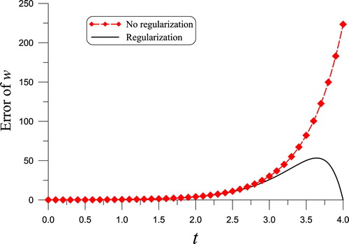n Figure 1 we plot the following errors in the time interval of $t\in [0,4]$: (48) $\text{Error 1}:=|w_e\left(t\right)-w_{nr}\left(t\right)|,\text{Error 2}:=|w_e\left(t\right)-w_r\left(t\right)|.$(48) It can be seen that the error of the regularized solution is much smaller than that without considering regularization. When the Error 1 exponentially grows with time, the Error 2 tends to zero. From this fact, the regularization effect is prominent.

Figure 1. Comparing the errors of solution without regularization and one with regularization to the exact solution of an unstable second-order ODE.

6. A simple regularization technique

Let (49) ${\text{β}}_{ij}=\sqrt{\lambda +{\mu }_{ij}}>0.$(49) Solving the ODEs in Equation (27(27) $T_{ij}^{″}\left(z\right)=({\mu }_{ij}+\lambda )T_{ij}\left(z\right)+F_{ij}(z,t+\mathrm{\Delta }t),$(27) ) endowing with the initial conditions (30(30) $\begin{array}{rl}& T_{ij}\left(0\right)=\frac{4}{ab}{\int }_0^b{\int }_0^a\left[h_5\right(\xi ,\zeta ,t+\mathrm{\Delta }t)-B(\xi ,\zeta ,0,t+\mathrm{\Delta }t\left)\right]\sin \frac{i\pi \xi }{a}\sin \frac{j\pi \zeta }{b}\mathrm{d}\xi \mathrm{d}\zeta ,\end{array}$(30) ) and (31(31) $\begin{array}{rl}& T_{ij}^{\prime }\left(0\right)=\frac{4}{ab}{\int }_0^b{\int }_0^a\left[h_6\right(\xi ,\zeta ,t+\mathrm{\Delta }t)-B_z(\xi ,\zeta ,0,t+\mathrm{\Delta }t\left)\right]\sin \frac{i\pi \xi }{a}\sin \frac{j\pi \zeta }{b}\mathrm{d}\xi \mathrm{d}\zeta .\end{array}$(31) ), we can derive (50) $\begin{array}{rl}{T}_{ij}\left(z\right)& =\frac{1}{{\text{β}}_{ij}}{\int }_0^z\sinh \left[{\text{β}}_{ij}\right(z-\tau \left)\right]F_{ij}(\tau ,t+\mathrm{\Delta }t)\mathrm{d}\tau +T_{ij}\left(0\right)\cosh \left({\text{β}}_{ij}z\right)\\ & +\frac{1}{{\text{β}}_{ij}}{T}_{ij}^{\prime }\left(0\right)\sinh \left({\text{β}}_{ij}z\right),\end{array}$(50) such that by Equation (23(23) $v(x,y,z,t+\mathrm{\Delta }t)=\sum _{i=1}^{\mathrm{\infty }}\sum _{j=1}^{\mathrm{\infty }}{T}_{ij}\left(z\right)\sin \frac{i\pi x}{a}\sin \frac{j\pi y}{b},$(23) ) the 2D Fourier sine series solution of Equations (14(14) $\begin{array}{rl}& v_{xx}(x,y,z,t+\mathrm{\Delta }t)+v_{yy}(x,y,z,t+\mathrm{\Delta }t)+v_{zz}(x,y,z,t+\mathrm{\Delta }t)\\ & =\lambda v(x,y,z,t+\mathrm{\Delta }t)+F(x,y,z,t+\mathrm{\Delta }t),\end{array}$(14) )–(17(17) $\begin{array}{rl}{v}_z(x,y,0,t+\mathrm{\Delta }t)& =h_6(x,y,t+\mathrm{\Delta }t)-B_z(x,y,0,t+\mathrm{\Delta }t),\end{array}$(17) ) is obtained as follows: (51) $v(x,y,z,t+\mathrm{\Delta }t)=\sum _{i=1}^n\sum _{j=1}^n{T}_{ij}\left(z\right)\sin \frac{i\pi x}{a}\sin \frac{j\pi y}{b}.$(51) In a practical use of the series solution, only $n^2$ finite terms in Equation (51(51) $v(x,y,z,t+\mathrm{\Delta }t)=\sum _{i=1}^n\sum _{j=1}^n{T}_{ij}\left(z\right)\sin \frac{i\pi x}{a}\sin \frac{j\pi y}{b}.$(51) ) are employed.

In order to recover the unknown Dirichlet data $u(x,y,c,t+\mathrm{\Delta }t)$ on the top of the cuboid, we can insert Equations (51(51) $v(x,y,z,t+\mathrm{\Delta }t)=\sum _{i=1}^n\sum _{j=1}^n{T}_{ij}\left(z\right)\sin \frac{i\pi x}{a}\sin \frac{j\pi y}{b}.$(51) ) and (50(50) $\begin{array}{rl}{T}_{ij}\left(z\right)& =\frac{1}{{\text{β}}_{ij}}{\int }_0^z\sinh \left[{\text{β}}_{ij}\right(z-\tau \left)\right]F_{ij}(\tau ,t+\mathrm{\Delta }t)\mathrm{d}\tau +T_{ij}\left(0\right)\cosh \left({\text{β}}_{ij}z\right)\\ & +\frac{1}{{\text{β}}_{ij}}{T}_{ij}^{\prime }\left(0\right)\sinh \left({\text{β}}_{ij}z\right),\end{array}$(50) ) into Equation (13(13) $v(x,y,z,t+\mathrm{\Delta }t)=u(x,y,z,t+\mathrm{\Delta }t)-B(x,y,z,t+\mathrm{\Delta }t).$(13) ) with z = c, obtaining (52) $u(x,y,c,t+\mathrm{\Delta }t)=B(x,y,c,t+\mathrm{\Delta }t)+\sum _{i=1}^n\sum _{j=1}^n{T}_{ij}\left(c\right)\sin \frac{i\pi x}{a}\sin \frac{j\pi y}{b},$(52) where (53) $\begin{array}{rl}{T}_{ij}\left(c\right)& =\frac{4}{ab{\text{β}}_{ij}}{\int }_0^c{\int }_0^b{\int }_0^a\sinh \left[{\text{β}}_{ij}\right(c-\tau \left)\right]F(\xi ,\zeta ,\tau ,t+\mathrm{\Delta }t)\sin \frac{i\pi \xi }{a}\sin \frac{j\pi \zeta }{b}\mathrm{d}\xi \mathrm{d}\zeta \mathrm{d}\tau \\ & +T_{ij}\left(0\right)\cosh \left({\text{β}}_{ij}c\right)+\frac{1}{{\text{β}}_{ij}}{T}_{ij}^{\prime }\left(0\right)\sinh \left({\text{β}}_{ij}c\right).\end{array}$(53) Notice that the factor $\exp \left({\text{β}}_{ij}c\right)$ in $\cosh \left({\text{β}}_{ij}c\right)$ and $\sinh \left({\text{β}}_{ij}c\right)$ may cause the ill-posedness to find $T_{ij}\left(c\right)$, when the input data $h_5(x,y)$ and $h_6(x,y)$ are polluted by large noise, which may greatly amplify the errors in the three terms in Equation (53(53) $\begin{array}{rl}{T}_{ij}\left(c\right)& =\frac{4}{ab{\text{β}}_{ij}}{\int }_0^c{\int }_0^b{\int }_0^a\sinh \left[{\text{β}}_{ij}\right(c-\tau \left)\right]F(\xi ,\zeta ,\tau ,t+\mathrm{\Delta }t)\sin \frac{i\pi \xi }{a}\sin \frac{j\pi \zeta }{b}\mathrm{d}\xi \mathrm{d}\zeta \mathrm{d}\tau \\ & +T_{ij}\left(0\right)\cosh \left({\text{β}}_{ij}c\right)+\frac{1}{{\text{β}}_{ij}}{T}_{ij}^{\prime }\left(0\right)\sinh \left({\text{β}}_{ij}c\right).\end{array}$(53) ), when i, j are large and hence ${\text{β}}_{ij}c$ are large. Therefore, we consider a simple regularization technique as demonstrated in Section 5 to $T_{ij}\left(c\right)$ by adding a regularization factor α as follows: (54) $\begin{array}{rl}{T}_{ij}\left(c\right)& =\frac{2}{ab{\text{β}}_{ij}}{\int }_0^c{\int }_0^b{\int }_0^a\left[\frac{e^{-{\text{β}}_{ij}\tau }}{e^{-{\text{β}}_{ij}c}+\alpha }-e^{-{\text{β}}_{ij}(c-\tau )}\right]\\ & \times F(\xi ,\zeta ,\tau ,t+\mathrm{\Delta }t)\sin \frac{i\pi \xi }{a}\sin \frac{j\pi \zeta }{b}\mathrm{d}\xi \mathrm{d}\zeta \mathrm{d}\tau \\ & +\frac{1}{2}{T}_{ij}\left(0\right)\left[\frac{1}{e^{-{\text{β}}_{ij}c}+\alpha }+e^{-{\text{β}}_{ij}c}\right]+\frac{1}{2{\text{β}}_{ij}}{T}_{ij}^{\prime }\left(0\right)\left[\frac{1}{e^{-{\text{β}}_{ij}c}+\alpha }-e^{-{\text{β}}_{ij}c}\right].\end{array}$(54) When $\alpha =0$, Equation (54(54) $\begin{array}{rl}{T}_{ij}\left(c\right)& =\frac{2}{ab{\text{β}}_{ij}}{\int }_0^c{\int }_0^b{\int }_0^a\left[\frac{e^{-{\text{β}}_{ij}\tau }}{e^{-{\text{β}}_{ij}c}+\alpha }-e^{-{\text{β}}_{ij}(c-\tau )}\right]\\ & \times F(\xi ,\zeta ,\tau ,t+\mathrm{\Delta }t)\sin \frac{i\pi \xi }{a}\sin \frac{j\pi \zeta }{b}\mathrm{d}\xi \mathrm{d}\zeta \mathrm{d}\tau \\ & +\frac{1}{2}{T}_{ij}\left(0\right)\left[\frac{1}{e^{-{\text{β}}_{ij}c}+\alpha }+e^{-{\text{β}}_{ij}c}\right]+\frac{1}{2{\text{β}}_{ij}}{T}_{ij}^{\prime }\left(0\right)\left[\frac{1}{e^{-{\text{β}}_{ij}c}+\alpha }-e^{-{\text{β}}_{ij}c}\right].\end{array}$(54) ) reduces to Equation (53(53) $\begin{array}{rl}{T}_{ij}\left(c\right)& =\frac{4}{ab{\text{β}}_{ij}}{\int }_0^c{\int }_0^b{\int }_0^a\sinh \left[{\text{β}}_{ij}\right(c-\tau \left)\right]F(\xi ,\zeta ,\tau ,t+\mathrm{\Delta }t)\sin \frac{i\pi \xi }{a}\sin \frac{j\pi \zeta }{b}\mathrm{d}\xi \mathrm{d}\zeta \mathrm{d}\tau \\ & +T_{ij}\left(0\right)\cosh \left({\text{β}}_{ij}c\right)+\frac{1}{{\text{β}}_{ij}}{T}_{ij}^{\prime }\left(0\right)\sinh \left({\text{β}}_{ij}c\right).\end{array}$(53) ).

By the same token, we can recover the solution $u(x,y,z,t+\mathrm{\Delta }t)$ in the whole domain under the Cauchy boundary conditions by (55) $u(x,y,z,t+\mathrm{\Delta }t)=B(x,y,z,t+\mathrm{\Delta }t)+\sum _{i=1}^n\sum _{j=1}^n{T}_{ij}\left(z\right)\sin \frac{i\pi x}{a}\sin \frac{j\pi y}{b},$(55) where (56) $\begin{array}{rl}{T}_{ij}\left(z\right)& =\frac{2}{ab{\text{β}}_{ij}}{\int }_0^z{\int }_0^b{\int }_0^a\left[\frac{e^{-{\text{β}}_{ij}\tau }}{e^{-{\text{β}}_{ij}z}+\alpha }-e^{-{\text{β}}_{ij}(z-\tau )}\right]\\ & \times F(\xi ,\zeta ,\tau ,t+\mathrm{\Delta }t)\sin \frac{i\pi \xi }{a}\sin \frac{j\pi \zeta }{b}\mathrm{d}\xi \mathrm{d}\zeta \mathrm{d}\tau \\ & +\frac{1}{2}{T}_{ij}\left(0\right)\left[\frac{1}{e^{-{\text{β}}_{ij}z}+\alpha }+e^{-{\text{β}}_{ij}z}\right]+\frac{1}{2{\text{β}}_{ij}}{T}_{ij}^{\prime }\left(0\right)\left[\frac{1}{e^{-{\text{β}}_{ij}z}+\alpha }-e^{-{\text{β}}_{ij}z}\right].\end{array}$(56) By updating the value of u sequentially, we can obtain the whole solutions $u(,x,y,z,t_{\ell })$ in a series of time sequence $t_{\ell }=\ell t_f/N_t$, where $N_t$ is the number of total time steps.

Theorem 6.1

Under the regularity assumptions (8(8) $\begin{array}{rl}& |S(x,y,z,t)|\le S_0,(x,y,z,t)\in \overline{\mathrm{\Omega }},\end{array}$(8) )–(10(10) $|f(x,y,z)|\le f_0$(10) ), $T_{ij}\left(c\right)$ in Equation (54(54) $\begin{array}{rl}{T}_{ij}\left(c\right)& =\frac{2}{ab{\text{β}}_{ij}}{\int }_0^c{\int }_0^b{\int }_0^a\left[\frac{e^{-{\text{β}}_{ij}\tau }}{e^{-{\text{β}}_{ij}c}+\alpha }-e^{-{\text{β}}_{ij}(c-\tau )}\right]\\ & \times F(\xi ,\zeta ,\tau ,t+\mathrm{\Delta }t)\sin \frac{i\pi \xi }{a}\sin \frac{j\pi \zeta }{b}\mathrm{d}\xi \mathrm{d}\zeta \mathrm{d}\tau \\ & +\frac{1}{2}{T}_{ij}\left(0\right)\left[\frac{1}{e^{-{\text{β}}_{ij}c}+\alpha }+e^{-{\text{β}}_{ij}c}\right]+\frac{1}{2{\text{β}}_{ij}}{T}_{ij}^{\prime }\left(0\right)\left[\frac{1}{e^{-{\text{β}}_{ij}c}+\alpha }-e^{-{\text{β}}_{ij}c}\right].\end{array}$(54) ) is bounded by (57) $|T_{ij}\left(c\right)|<C_3,$(57) where $C_3$ is a constant; hence, the numerically regularized solution $u(x,y,c,t+\mathrm{\Delta }t)$ in Equation (52(52) $u(x,y,c,t+\mathrm{\Delta }t)=B(x,y,c,t+\mathrm{\Delta }t)+\sum _{i=1}^n\sum _{j=1}^n{T}_{ij}\left(c\right)\sin \frac{i\pi x}{a}\sin \frac{j\pi y}{b},$(52) ) is stable with (58) $|u(x,y,c,t+\mathrm{\Delta }t)|<u_0,(x,y,c,t+\mathrm{\Delta }t)\in \overline{\mathrm{\Omega }},$(58) where $u_0$ is a constant. Moreover, the solution $u(x,y,z,t+\mathrm{\Delta }t)$ in Equation (55(55) $u(x,y,z,t+\mathrm{\Delta }t)=B(x,y,z,t+\mathrm{\Delta }t)+\sum _{i=1}^n\sum _{j=1}^n{T}_{ij}\left(z\right)\sin \frac{i\pi x}{a}\sin \frac{j\pi y}{b},$(55) ) is stable.

Proof.

We begin with t = 0 and prove the results at $t=\mathrm{\Delta }t$. Then, in a sequence of time steps we can prove this theorem for all time $t\le t_f$. Under the regularity assumptions (8(8) $\begin{array}{rl}& |S(x,y,z,t)|\le S_0,(x,y,z,t)\in \overline{\mathrm{\Omega }},\end{array}$(8) )–(10(10) $|f(x,y,z)|\le f_0$(10) ) and using $u(x,y,z,0)=f(x,y,z)$ in Equation (10(10) $|f(x,y,z)|\le f_0$(10) ), from Equations (18(18) $\begin{array}{rl}F(x,y,z,t+\mathrm{\Delta }t)& =\lambda B(x,y,z,t+\mathrm{\Delta }t)-S(x,y,z,t+\mathrm{\Delta }t)-\lambda u(x,y,z,t)\\ & -B_{xx}(x,y,z,t+\mathrm{\Delta }t)-B_{yy}(x,y,z,t+\mathrm{\Delta }t)-B_{zz}(x,y,z,t+\mathrm{\Delta }t).\end{array}$(18) ), (8(8) $\begin{array}{rl}& |S(x,y,z,t)|\le S_0,(x,y,z,t)\in \overline{\mathrm{\Omega }},\end{array}$(8) ) and (11(11) $B(x,y,z,t)\in {\mathcal{C}}^2\left(\overline{\mathrm{\Omega }}\right)\Rightarrow |B(x,y,z,t)|\le B_0,(x,y,z,t)\in \overline{\mathrm{\Omega }},$(11) ) it follows that (59) $|F(x,y,z,\mathrm{\Delta }t)|\le F_0,$(59) where $F_0$ is a constant.

Due to ${\mu }_{ij}>0$ as shown by Equation (28(28) $\begin{array}{rl}& {\mu }_{ij}:={\left(\frac{i\pi }{a}\right)}^2+{\left(\frac{j\pi }{b}\right)}^2,\end{array}$(28) ), ${\text{β}}_{ij}$ in Equation (49(49) ${\text{β}}_{ij}=\sqrt{\lambda +{\mu }_{ij}}>0.$(49) ) satisfies (60) $0<\frac{1}{{\text{β}}_{ij}}<\sqrt{\mathrm{\Delta }t}.$(60) The following inequalities are apparent: (61) $\begin{array}{rl}& \frac{e^{-{\text{β}}_{ij}\tau }}{e^{-{\text{β}}_{ij}c}+\alpha }-e^{-{\text{β}}_{ij}(c-\tau )}<\frac{e^{-{\text{β}}_{ij}\tau }}{e^{-{\text{β}}_{ij}c}+\alpha }<\frac{1}{e^{-{\text{β}}_{ij}c}+\alpha }<\frac{1}{\alpha },\end{array}$(61) (62) $\begin{array}{rl}& \frac{1}{e^{-{\text{β}}_{ij}c}+\alpha }+e^{-{\text{β}}_{ij}c}<\frac{1}{e^{-{\text{β}}_{ij}c}+\alpha }+1<\frac{1+\alpha }{\alpha },\end{array}$(62) (63) $\begin{array}{rl}& \frac{1}{e^{-{\text{β}}_{ij}c}+\alpha }-e^{-{\text{β}}_{ij}c}<\frac{1}{e^{-{\text{β}}_{ij}c}+\alpha }<\frac{1}{\alpha }.\end{array}$(63) From Equations (54(54) $\begin{array}{rl}{T}_{ij}\left(c\right)& =\frac{2}{ab{\text{β}}_{ij}}{\int }_0^c{\int }_0^b{\int }_0^a\left[\frac{e^{-{\text{β}}_{ij}\tau }}{e^{-{\text{β}}_{ij}c}+\alpha }-e^{-{\text{β}}_{ij}(c-\tau )}\right]\\ & \times F(\xi ,\zeta ,\tau ,t+\mathrm{\Delta }t)\sin \frac{i\pi \xi }{a}\sin \frac{j\pi \zeta }{b}\mathrm{d}\xi \mathrm{d}\zeta \mathrm{d}\tau \\ & +\frac{1}{2}{T}_{ij}\left(0\right)\left[\frac{1}{e^{-{\text{β}}_{ij}c}+\alpha }+e^{-{\text{β}}_{ij}c}\right]+\frac{1}{2{\text{β}}_{ij}}{T}_{ij}^{\prime }\left(0\right)\left[\frac{1}{e^{-{\text{β}}_{ij}c}+\alpha }-e^{-{\text{β}}_{ij}c}\right].\end{array}$(54) ), (59(59) $|F(x,y,z,\mathrm{\Delta }t)|\le F_0,$(59) ), (32(32) $|T_{ij}\left(0\right)|\le C_1,|T_{ij}^{\prime }\left(0\right)|\le C_2,$(32) ) and (60(60) $0<\frac{1}{{\text{β}}_{ij}}<\sqrt{\mathrm{\Delta }t}.$(60) )–(63(63) $\begin{array}{rl}& \frac{1}{e^{-{\text{β}}_{ij}c}+\alpha }-e^{-{\text{β}}_{ij}c}<\frac{1}{e^{-{\text{β}}_{ij}c}+\alpha }<\frac{1}{\alpha }.\end{array}$(63) ), it follows that (64) $|T_{ij}\left(c\right)|<\frac{2c{F}_0\sqrt{\mathrm{\Delta }t}}{\alpha }+\frac{(1+\alpha )C_1}{2\alpha }+\frac{C_2\sqrt{\mathrm{\Delta }t}}{2\alpha }.$(64) In general, $\sqrt{\mathrm{\Delta }t}$ is a small time increment and α is a finite regularization parameter. Upon letting $C_3$ be the right-hand side, Equation (57(57) $|T_{ij}\left(c\right)|<C_3,$(57) ) is proved. Equation (58(58) $|u(x,y,c,t+\mathrm{\Delta }t)|<u_0,(x,y,c,t+\mathrm{\Delta }t)\in \overline{\mathrm{\Omega }},$(58) ) is easily proved by using Equations (57(57) $|T_{ij}\left(c\right)|<C_3,$(57) ), (11(11) $B(x,y,z,t)\in {\mathcal{C}}^2\left(\overline{\mathrm{\Omega }}\right)\Rightarrow |B(x,y,z,t)|\le B_0,(x,y,z,t)\in \overline{\mathrm{\Omega }},$(11) ) and (55(55) $u(x,y,z,t+\mathrm{\Delta }t)=B(x,y,z,t+\mathrm{\Delta }t)+\sum _{i=1}^n\sum _{j=1}^n{T}_{ij}\left(z\right)\sin \frac{i\pi x}{a}\sin \frac{j\pi y}{b},$(55) ) (65) $|u(x,y,c,\mathrm{\Delta }t)|<B_0+n^2{C}_3,u_0:=B_0+n^2{C}_3.$(65) Then, we can go to next time step with t = 0 replaced by $\mathrm{\Delta }t$ and $\mathrm{\Delta }t$ replaced by $2\mathrm{\Delta }t$ and using the boundedness of $|u(x,y,c,\mathrm{\Delta }t)|<u_0$ as just proved in the previous step and with $|F(x,y,c,2\mathrm{\Delta }t)|<F_0$ to replace Equation (59(59) $|F(x,y,z,\mathrm{\Delta }t)|\le F_0,$(59) ). The proof of the stability of $u(x,y,z,\mathrm{\Delta }t)$ in Equation (55(55) $u(x,y,z,t+\mathrm{\Delta }t)=B(x,y,z,t+\mathrm{\Delta }t)+\sum _{i=1}^n\sum _{j=1}^n{T}_{ij}\left(z\right)\sin \frac{i\pi x}{a}\sin \frac{j\pi y}{b},$(55) ) is similar. Thus, we end the proof of this theorem.

Remark 6.1

The presented algorithm for solving the 3D SHE has some advantages. The solution $u(x,y,c,t+\mathrm{\Delta }t)$ as shown in Equation (52(52) $u(x,y,c,t+\mathrm{\Delta }t)=B(x,y,c,t+\mathrm{\Delta }t)+\sum _{i=1}^n\sum _{j=1}^n{T}_{ij}\left(c\right)\sin \frac{i\pi x}{a}\sin \frac{j\pi y}{b},$(52) ) automatically satisfies the boundary conditions in Equation (3(3) $\begin{array}{rl}& \begin{array}{l}u(0,y,z,t)=h_1(y,z,t),u(a,y,z,t)=h_2(y,z,t),u(x,0,z,t)=h_3(x,z,t),\\ u(x,b,z,t)=h_4(x,z,t),u(x,y,0,t)=h_5(x,y,t),u_z(x,y,0,t)=h_6(x,y,t),\end{array}\end{array}$(3) ). The boundary information has been incorporated into $u(x,y,c,t+\mathrm{\Delta }t)$ through the homogenization function $B(x,y,c,t+\mathrm{\Delta }t)$. The accuracy is very good, although we merely adopt a few sine series to approximate $u(x,y,c,t+\mathrm{\Delta }t)$, which is reflected in a small number n in Equation (52(52) $u(x,y,c,t+\mathrm{\Delta }t)=B(x,y,c,t+\mathrm{\Delta }t)+\sum _{i=1}^n\sum _{j=1}^n{T}_{ij}\left(c\right)\sin \frac{i\pi x}{a}\sin \frac{j\pi y}{b},$(52) ). The numerical method provides a semi-analytical solution.

7. Numerical tests of the 3D SHEs

For the inverse Cauchy problems of the 3D SHE, we assume that the given boundary data are polluted by a random noise (66) $\begin{array}{rl}& {\hat{h}}_5(x_i,y_j,z_k,t_{\ell })=h_5(x_i,y_j,z_k,t_{\ell })+sR(i,j,k,t_{\ell }),\end{array}$(66) (67) $\begin{array}{rl}& {\hat{h}}_6(x_i,y_j,z_k,t_{\ell })=h_6(x_i,y_j,z_k,t_{\ell })+sR(i,j,k,t_{\ell }),\end{array}$(67) where s is the intensity of noise and $R(i,j,k,t_{\ell })\in [-1,1]$ are random numbers.

In order to assess the performance of the newly developed algorithm, let us investigate the following examples. Sometimes the closed-form solutions are available, which can be used to assess the errors of numerical solutions. Besides the usual absolute error defined at the grid points $(x_i,y_j)=\left(ia/\right(N+1),jb/(N+1\left)\right),i,j=1,\dots ,N$, we will employ the maximum error to evaluate the error of numerical solution by (68) $\text{maximum error}:=\underset{i,j=1,\dots ,N}{max}|u_n(x_i,y_j,c,t)-u_e(x_i,y_j,c,t)|,$(68) where $u_n(x_i,y_j,c,t)$ and $u_e(x_i,y_j,c,t)$ are, respectively, the numerical solution and the exact solution of $u(x,y,z,t)$ at the $(i,j)$th grid point on the plane z = c and at the time t. Below we take N = 20 for all cases.

If $\alpha =0$ can generate good solution, we do not need to consider regularization. Otherwise, we need to consider α and n in Equation (52(52) $u(x,y,c,t+\mathrm{\Delta }t)=B(x,y,c,t+\mathrm{\Delta }t)+\sum _{i=1}^n\sum _{j=1}^n{T}_{ij}\left(c\right)\sin \frac{i\pi x}{a}\sin \frac{j\pi y}{b},$(52) ). If there exists no noise, basically the semi-analytic solution approaches to the exact one. Under a noise s, we expect that the accuracy can be kept in the same order $A_{0}s$, where $A_0>0$. If a noise s is imposed on $T_{ij}\left(0\right)$, $T_{ij}^{\prime }\left(0\right)$ and $F(\xi ,\zeta ,\tau ,t+\mathrm{\Delta }t)$, by Equation (54(54) $\begin{array}{rl}{T}_{ij}\left(c\right)& =\frac{2}{ab{\text{β}}_{ij}}{\int }_0^c{\int }_0^b{\int }_0^a\left[\frac{e^{-{\text{β}}_{ij}\tau }}{e^{-{\text{β}}_{ij}c}+\alpha }-e^{-{\text{β}}_{ij}(c-\tau )}\right]\\ & \times F(\xi ,\zeta ,\tau ,t+\mathrm{\Delta }t)\sin \frac{i\pi \xi }{a}\sin \frac{j\pi \zeta }{b}\mathrm{d}\xi \mathrm{d}\zeta \mathrm{d}\tau \\ & +\frac{1}{2}{T}_{ij}\left(0\right)\left[\frac{1}{e^{-{\text{β}}_{ij}c}+\alpha }+e^{-{\text{β}}_{ij}c}\right]+\frac{1}{2{\text{β}}_{ij}}{T}_{ij}^{\prime }\left(0\right)\left[\frac{1}{e^{-{\text{β}}_{ij}c}+\alpha }-e^{-{\text{β}}_{ij}c}\right].\end{array}$(54) ), $T_{ij}\left(c\right)$ will have an error due to s, when we suppose that other integration errors can be neglected. As shown in Equation (54(54) $\begin{array}{rl}{T}_{ij}\left(c\right)& =\frac{2}{ab{\text{β}}_{ij}}{\int }_0^c{\int }_0^b{\int }_0^a\left[\frac{e^{-{\text{β}}_{ij}\tau }}{e^{-{\text{β}}_{ij}c}+\alpha }-e^{-{\text{β}}_{ij}(c-\tau )}\right]\\ & \times F(\xi ,\zeta ,\tau ,t+\mathrm{\Delta }t)\sin \frac{i\pi \xi }{a}\sin \frac{j\pi \zeta }{b}\mathrm{d}\xi \mathrm{d}\zeta \mathrm{d}\tau \\ & +\frac{1}{2}{T}_{ij}\left(0\right)\left[\frac{1}{e^{-{\text{β}}_{ij}c}+\alpha }+e^{-{\text{β}}_{ij}c}\right]+\frac{1}{2{\text{β}}_{ij}}{T}_{ij}^{\prime }\left(0\right)\left[\frac{1}{e^{-{\text{β}}_{ij}c}+\alpha }-e^{-{\text{β}}_{ij}c}\right].\end{array}$(54) ), the major contribution to enlarge the error in $T_{jk}\left(c\right)$ is the term with i = j = n. Then, when we use the regularization principle demonstrated in Section 5, and integrate the first term in Equation (54(54) $\begin{array}{rl}{T}_{ij}\left(c\right)& =\frac{2}{ab{\text{β}}_{ij}}{\int }_0^c{\int }_0^b{\int }_0^a\left[\frac{e^{-{\text{β}}_{ij}\tau }}{e^{-{\text{β}}_{ij}c}+\alpha }-e^{-{\text{β}}_{ij}(c-\tau )}\right]\\ & \times F(\xi ,\zeta ,\tau ,t+\mathrm{\Delta }t)\sin \frac{i\pi \xi }{a}\sin \frac{j\pi \zeta }{b}\mathrm{d}\xi \mathrm{d}\zeta \mathrm{d}\tau \\ & +\frac{1}{2}{T}_{ij}\left(0\right)\left[\frac{1}{e^{-{\text{β}}_{ij}c}+\alpha }+e^{-{\text{β}}_{ij}c}\right]+\frac{1}{2{\text{β}}_{ij}}{T}_{ij}^{\prime }\left(0\right)\left[\frac{1}{e^{-{\text{β}}_{ij}c}+\alpha }-e^{-{\text{β}}_{ij}c}\right].\end{array}$(54) ), we can derive (69) $\frac{8s}{(e^{-{\text{β}}_{nn}c}+\alpha ){\text{β}}_{nn}^2{n}^2{\pi }^2}+\frac{1}{2(e^{-{\text{β}}_{nn}c}+\alpha )}+\frac{1}{2{\text{β}}_{nn}(e^{-{\text{β}}_{nn}c}+\alpha )}=A_{0}s,$(69) where (70) ${\text{β}}_{nn}=\sqrt{\lambda +\frac{n^2{\pi }^2}{a^2}+\frac{n^2{\pi }^2}{b^2}}.$(70) By Equation (69(69) $\frac{8s}{(e^{-{\text{β}}_{nn}c}+\alpha ){\text{β}}_{nn}^2{n}^2{\pi }^2}+\frac{1}{2(e^{-{\text{β}}_{nn}c}+\alpha )}+\frac{1}{2{\text{β}}_{nn}(e^{-{\text{β}}_{nn}c}+\alpha )}=A_{0}s,$(69) ), it follows that (71) $\begin{array}{rl}\alpha & =\frac{1}{A_0}\left[\frac{8}{{\text{β}}_{nn}^2{n}^2{\pi }^2}+\frac{1}{2}+\frac{1}{2{\text{β}}_{nn}}\right]-e^{-{\text{β}}_{nn}c}\\ & ={\text{β}}_0\left[\frac{8}{{\text{β}}_{nn}^2{n}^2{\pi }^2}+\frac{1}{2}+\frac{1}{2{\text{β}}_{nn}}\right]e^{-{\text{β}}_{nn}c}-e^{-{\text{β}}_{nn}c},\end{array}$(71) where we have taken $A_0=e^{{\text{β}}_{nn}c}/{\text{β}}_0$ and ${\text{β}}_0$ is some constant.

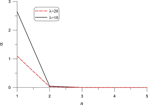
With the parameters $a=b=c=t_f=1$ and ${\text{β}}_0=1000$, we plot the curves of α vs. n in Figure 2 for different time step sizes $\mathrm{\Delta }t=0.1$ and $\mathrm{\Delta }t=0.05$, such that $\lambda =1/\mathrm{\Delta }t=10$ and $\lambda =1/\mathrm{\Delta }t=20$. When n increases, α tends to stable value $9.38\times {10}^{-8}$ for $\lambda =10$ and $7.51\times {10}^{-8}$ for $\lambda =20$. Below, we may select α basing on this formula.

Figure 2. The regularization parameter vs. n for different time step sizes.

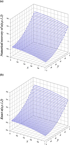
7.1. Example 1

First, we consider (72) $u(x,y,z,t)=e^{-t}(y^2-x^2-z^2),S(x,y,z,t)=e^{-t}(2+x^2-y^2-z^2).$(72) In a spatial temporal domain with $a=1,b=2,c=1$, $t_f=2$ and $N_t=5$, hence $\lambda =N_t/t_f=2.5$, and under a large noise with s = 0.2 and n = 2, we recover the Dirichlet data $u(x,y,z,t)$ on the plane z = 1 at the final time, where we take $\alpha =2$. As shown in Figure 3(a,b) for the comparison of the numerical result and exact solution of $u(x,y,z,t)$ on the plane z = 1, we have obtained a very accurate solution with the maximum error being $5.11\times {10}^{-3}$. For this example the CPU time is 16.05 s.

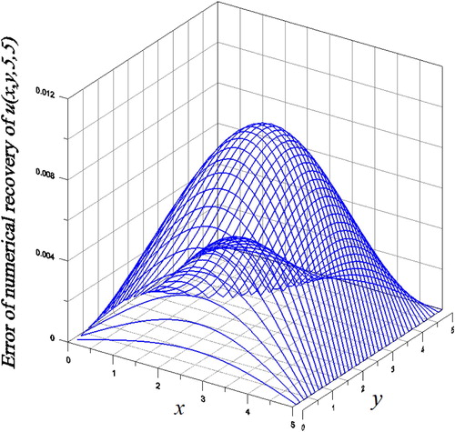
Figure 3. For Example 1 of the inverse Cauchy problem of 3D heat equation solved by the 2D Fourier sine series method with spring-damping regularization, comparing (a) numerical and (b) exact solutions on the plane z = 1 at the final time.

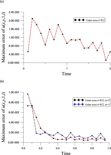
In Figure 4(a), we plot the time histories of the maximum error of $u(x,y,z,t)$ on the plane z = 1, where the parameters are the same, besides $N_t=20$. Because we are calculating the maximum errors at total 20 discretized times, the CPU time is raised to 72.79 s. It is interesting that the errors are all smaller than $2.1\times {10}^{-2}$. It indicates that the presented regularized Fourier sine series method is accurate and stable.

Figure 4. For (a) Example 1 and (b) Example 2 of the inverse Cauchy problems of 3D heat equation solved by the 2D Fourier sine series method with spring-damping regularization, showing the maximum errors on the plane z = 1 in time.

We consider a larger spatial domain with $a=10,b=5,c=1$, and the regularization parameter α is calculated from Equation (71(71) $\begin{array}{rl}\alpha & =\frac{1}{A_0}\left[\frac{8}{{\text{β}}_{nn}^2{n}^2{\pi }^2}+\frac{1}{2}+\frac{1}{2{\text{β}}_{nn}}\right]-e^{-{\text{β}}_{nn}c}\\ & ={\text{β}}_0\left[\frac{8}{{\text{β}}_{nn}^2{n}^2{\pi }^2}+\frac{1}{2}+\frac{1}{2{\text{β}}_{nn}}\right]e^{-{\text{β}}_{nn}c}-e^{-{\text{β}}_{nn}c},\end{array}$(71) ) with ${\text{β}}_0=50$. In Table 1, we compare the maximum errors with regularization and without considering regularization. It can be seen that n = 2 is better than n = 1. Although for n = 1, we have obtained quite accurate solution with the maximum error being $5.105\times {10}^{-1}$, which is acceptable upon comparing with the maximum value $max|u(x,y,1,2)|=37.15$. Without considering regularization, the solution is unstable, which leads to an unreasonable maximum error 37.15 for n = 1 and the maximum error 180.463 for n = 2.

Table 1. For Example 1 ($a=10,b=5,c=1,t_f=2,N_t=10$), the maximum errors with regularization and without considering regularization ($\alpha =0$).

$n=1,\alpha =1.3943$	$n=2,\alpha =1.0076$	$\alpha =0,n=1$	$\alpha =0,n=2$
$5.105\times {10}^{-1}$	$3.878\times {10}^{-2}$	37.150	180.463

From n = 1 to n = 2, it can be seen that the convergence is very fast.

7.2. Example 2

Next, we consider (73) $u(x,y,z,t)=t+e^{-{\pi }^{2}t}[\cos (\pi x)+\cos (\pi y)+\cos (\pi z\left)\right],S(x,y,z,t)=1,$(73) in a large spatial temporal domain with $a=b=5,c=1$, $t_f=1$ and $N_t=20$, hence $\lambda =N_t/t_f=20$, where we take n = 2. The resulting modified Helmholtz equation is with a large wave number $\lambda =20$.

In Figure 4(b), we plot the time histories of the maximum error of $u(x,y,z,t)$ on the plane z = 1, where the parameters $\alpha =1$ and $\alpha =2$ are used. Because we are calculating the maximum errors at a total $N_t=20$ discretized times, the CPU times are, respectively, 106.1 s and 101.4 s. It is interesting that the value of α renders little influence. It indicates that the presented regularized Fourier sine series method is accurate and stable.

In a larger spatial temporal domain with a = b = c = 5, $t_f=5$ and $N_t=10$, and under a large noise with s = 0.2 and n = 2, we recover the Dirichlet data $u(x,y,z,t_f)$ on the plane z = 5 at the final time, where we take $\alpha =1$. As shown in Figure 5 for the absolute errors between the numerical result and exact solution of $u(x,y,z,t)$ on the plane z = 5, we have obtained a quite accurate solution with the maximum error being $1.088\times {10}^{-2}$. We notice the maximum value $max|u(x,y,1,5)|=5$. Although for the inverse Cauchy problem of the SHE with large spatial domain and large final time and under large noise, the presented algorithm led to good numerical solution with small error.

Figure 5. For Example 2 in a larger spatial domain, showing the errors on the plane z = 5 at the final time.

7.3. Example 3

Then, we consider a more complex case (74) $u(x,y,z,t)=e^{xyz\sin t},S(x,y,z,t)=[\cos t-(y^2{z}^2+x^2{z}^2+x^2{y}^2){\sin }^{2}t]e^{xyz\sin t}.$(74) In a spatial temporal domain with $a=1,b=2,c=1$, $t_f=2$ and $N_t=10$, hence $\lambda =N_t/t_f=5$, and under a large noise with s = 0.2 and n = 1, we recover the Dirichlet data $u(x,y,z,t)$ on the plane z = 1 at the final time, where we can take $\alpha =0$ due to n = 1. As shown in Figure 6(a,b) for the comparison of the numerical result and the exact solution of $u(x,y,z,t)$ on the plane z = 1, we have obtained quite accurate solution with the maximum error being $2.03\times {10}^{-1}$, which is acceptable upon comparing with the maximum value $max|u(x,y,1,2)|=6.163$. For this example the CPU time is 9.86 s.

Figure 6. For Example 3 of the inverse Cauchy problem of 3D heat equation solved by the 2D Fourier sine series method with spring-damping regularization, comparing (a) numerical and (b) exact solutions on the plane z = 1 at the final time.

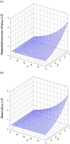
We consider a slightly larger spatial domain with $a=2,b=2,c=1$, and the regularization parameter α is calculated from Equation (71(71) $\begin{array}{rl}\alpha & =\frac{1}{A_0}\left[\frac{8}{{\text{β}}_{nn}^2{n}^2{\pi }^2}+\frac{1}{2}+\frac{1}{2{\text{β}}_{nn}}\right]-e^{-{\text{β}}_{nn}c}\\ & ={\text{β}}_0\left[\frac{8}{{\text{β}}_{nn}^2{n}^2{\pi }^2}+\frac{1}{2}+\frac{1}{2{\text{β}}_{nn}}\right]e^{-{\text{β}}_{nn}c}-e^{-{\text{β}}_{nn}c},\end{array}$(71) ) with ${\text{β}}_0=100$. In Table 2, we compare the maximum errors with regularization and without considering regularization. Without considering regularization, the solution is unstable, which leads to a maximum error 2.945 for n = 1 and the maximum error 12.413 for n = 2, which are not acceptable upon comparing with the maximum value $max|u(x,y,1,2)|=6.805$. With a suitable regularization parameter and although for n = 1, we have obtained quite accurate solution with the maximum error being $4.65\times {10}^{-1}$, which is acceptable upon comparing with the maximum value $max|u(x,y,1,2)|=6.805$. It can be seen that n = 2 and n = 3 are not better than n = 1.

Table 2. For Example 3 ($a=2,b=2,c=1,t_f=0.5,N_t=5$), the maximum errors with regularization and without considering regularization ($\alpha =0$).

$n=1,\alpha =1.4128$	$n=2,\alpha =0.25199$	$n=3,\alpha =0.035$	$\alpha =0,n=1$	$\alpha =0,n=2$
$4.650\times {10}^{-1}$	$6.336\times {10}^{-1}$	$9.122\times {10}^{-1}$	2.945	12.413

From Tables 1 and 2, we can observe that with small n the solution is quite accurate, which is due to the incorporation of the homogenization function in the solution, and thus merely adding a few Fourier sine series terms can produce a good approximation to the real solution, which renders the computational time very saving.

7.4. Example 4

Finally, we consider (75) $u(x,y,z,t)=e^{-{\pi }^{2}t}[\cos (\pi x)+\cos (\pi y)+\cos (\pi z\left)\right]+xyzt,S(x,y,z,t)=xyz,$(75) in a large spatial temporal domain with $a=b=20,c=5$, $t_f=0.1$ and $N_t=5$, hence $\lambda =N_t/t_f=50$. The resulting modified Helmholtz equation is with a large wave number $\lambda =50$.

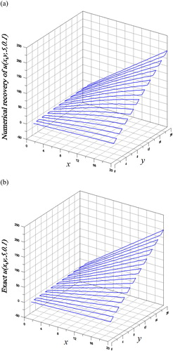
In the algorithm, we take n = 2 and $\alpha =3$. As shown in Figure 7(a,b) for the comparison of the numerical result and the exact solution of $u(x,y,z,t)$ on the plane z = 5, we have obtained quite accurate solution with the maximum error being 6.35, which is acceptable upon comparing with the maximum value $max|u(x,y,1,2)|=200.37$. For this example the CPU time is 27.44 s.

Figure 7. For Example 4 of the inverse Cauchy problem of 3D heat equation solved by the 2D Fourier sine series method with spring-damping regularization, comparing (a) numerical and (b) exact solutions on the plane z = 1 at the final time.

8. Conclusions

In the paper, we have solved the inverse Cauchy problems of the 3D sideways heat equation in a cuboid by a Fourier sine series method. The key steps are that we can transform the Cauchy problems of the 3D heat equation to the inverse Cauchy problems of the 3D modified Helmholtz equation, and then established a 2D time-dependent homogenization function, such that for the transformed variable we can derive its Fourier sine series solution, and determine the expansion coefficients in closed-form by taking advantage of the orthogonality of sinusoidal functions. We have derived a set of second-order ordinary differential equations, which can be solved in closed-form to determine the expansion coefficients. The 3D inverse Cauchy problems of the transient heat equation were solved stably through a simple spring-damping regularization technique by inserting the regularization parameter into the expansion coefficients, which results in a regularized 2D Fourier sine series solution. The analysis of the regularization parameter and the stability of solution was worked out. The novel method is accurate to find the numerical solutions, even a large noise up to $20\mathrm{\%}$ was imposed on the over-specified Neumann data. Due to the incorporation of the homogenization function in the solution, merely adding a few Fourier sine series terms can lead to accurate results, which renders the computational time very saving. The presented techniques of homogenization function and the stabilization of the unstable second-order ODEs by suitable regularization parameter are very powerful, which can be used in many engineering inverse problems with regular 2D or 3D domains. A recent result [39] was solving the 2D backward heat conduction problem. Some works about the 3D inverse Cauchy problems of elliptic type equations can be studied in the near future.

Disclosure statement

No potential conflict of interest was reported by the author(s).

References

- Beck JV, Blackwell B, Clair CRS. Inverse heat conduction: ill-posed problem. New York (NY): Wiley; 1985.
- Murio DA. The mollification method and the numerical solution of the inverse heat conduction problem by finite differences. Comput Math Appl. 1989;17:1385–1396. doi: 10.1016/0898-1221(89)90022-9
- Guo L, Murio DA, Roth C. A mollified space marching finite differences algorithm for the inverse heat conduction problem with slab symmetry. Comput Math Appl. 1990;19:75–89. doi: 10.1016/0898-1221(90)90196-Q
- Murio DA, Guo L. A stable space marching finite differences algorithm for the inverse heat conduction problem with no initial filtering procedure. Comput Math Appl. 1990;19:35–50. doi: 10.1016/0898-1221(90)90356-O
- Guo L, Murio DA. A mollified space-marching finite different algorithm for the two-dimensional inverse heat conduction problem with slab symmetry. Inverse Prob. 1991;7:247–259. doi: 10.1088/0266-5611/7/2/008
- Al-Khalidy N. On the solution of parabolic and hyperbolic inverse heat conduction problems. Int J Heat Mass Transf. 1998;41:3731–3740. doi: 10.1016/S0017-9310(98)00102-1
- Seidman TI, Eldén L. An ‘optimal filtering’ method for the sideways heat equation. Inverse Prob. 1990;6:681–696. doi: 10.1088/0266-5611/6/4/013
- Eldén L. Numerical solution of the sideways heat equation by difference approximation in time. Inverse Prob. 1995;11:913–923. doi: 10.1088/0266-5611/11/4/017
- Eldén L. Numerical solution of the sideways heat equation. In: Engl H, Rundell W, editors. Inverse problems in diffusion processes. Proceedings in applied mathematics. Philadelphia (PA): SIAM; 1995.
- Regińska T. Sideways heat equation and wavelets. J Comp Appl Math. 1995;63:209–214. doi: 10.1016/0377-0427(95)00073-9
- Regińska T, Eldén L. Solving the sideways heat equation by a wavelet-Galerkin method. Inverse Prob. 1997;13:1093–1106. doi: 10.1088/0266-5611/13/4/014
- Berntsson F. A spectral method for solving the sideways heat equation. Inverse Prob. 1999;15:891–906. doi: 10.1088/0266-5611/15/4/305
- Dorroh JR, Ru X. The application of the method of quasi-reversibility to the sideways heat equation. J Math Anal and Appl. 1999;15:503–519. doi: 10.1006/jmaa.1999.6462
- Eldén L, Berntsson F, Regińska T. Wavelet and Fourier methods for solving the sideways heat equation. SIAM J Sci Comput. 2000;21:2187–2205. doi: 10.1137/S1064827597331394
- Regińska T. Application of wavelet shrinkage to solving the sideways heat equation. BIT. 2001;41:1101–1110. doi: 10.1023/A:1021909816563
- Fu CL, Qiu CY, Zhu YB. A note on ‘sideways heat equation and wavelets’ and constant e∗. Comput Math Appl. 2002;43:1125–1134. doi: 10.1016/S0898-1221(02)80017-7
- Qiu CY, Fu CL, Zhu YB. Wavelets and regularization of the sideways heat equation. Comput Math Appl. 2003;46:821–829. doi: 10.1016/S0898-1221(03)90145-3
- Berntsson F. Sequential solution of the sideways heat equation by windowing of the data. Inverse Prob Sci Eng. 2003;11:91–103. doi: 10.1080/1068276021000048564
- Wang J. The multi-resolution method applied to the sideways heat equation. J Math Anal Appl. 2005;309:661–673. doi: 10.1016/j.jmaa.2004.11.025
- Xiong XT, Fu CL, Li HF. Fourier regularization method of a sideways heat equation for determining surface heat flux. J Math Anal Appl. 2006;317:331–348. doi: 10.1016/j.jmaa.2005.12.010
- Wang JR. Uniform convergence of wavelet solution to the sideways heat equation. Acta Math Sin-E. 2010;26:1981–1992. doi: 10.1007/s10114-010-7242-4
- Deng Y, Liu Z. New fast iteration for determining surface temperature and heat flux of general sideways parabolic equation. Nonl Anal Real World Appl. 2011;12:156–166. doi: 10.1016/j.nonrwa.2010.06.005
- Pakanen JE. A sequential one-dimensional solution for the sideways heat equation in a semi-infinite, finite and multilayer slab. Numer Heat Transfer B. 2012;61:471–491. doi: 10.1080/10407790.2012.687990
- Nguyen HT, Luu VCH. Two new regularization methods for solving sideways heat equation. J Inequal Appl. 2015;2015:65–81. doi: 10.1186/s13660-015-0564-0
- Chang CW, Liu CS, Chang J-R. A group preserving scheme for inverse heat conduction problems. Comput Model Eng Sci. 2005;10:13–38.
- Chang CW, Liu CH, Wang CC. Review of computational schemes in inverse heat conduction problems. Smart Sci. 2018;6:94–103. doi: 10.1080/23080477.2017.1408987
- Yu Y, Xu D, Hon YC. Reconstruction of inaccessible boundary value in a sideways parabolic problem with variable coefficients – forward collocation with finite integration method. Eng Anal Bound Elem. 2015;61:78–90. doi: 10.1016/j.enganabound.2015.07.007
- Liu CS. Homogenized functions to recover H(t)/H(x) by solving a small scale linear system of differencing equations. Int J Heat Mass Transf. 2016;101:1103–1110. doi: 10.1016/j.ijheatmasstransfer.2016.05.133
- Liu CS. To recover heat source G(x)+H(t) by using homogenized function and solving rectangular differencing equations. Numer Heat Transfer B. 2016;69:351–363. doi: 10.1080/10407790.2015.1125211
- Liu CS, Chen W, Lin J. A homogenized function to recover wave source by solving a small scale linear system of differencing equations. Comput Model Eng Sci. 2016;111:421–435.
- Liu CS, Qiu L, Wang F. Nonlinear wave inverse source problem solved by a method of m-order homogenization functions. Appl Math Lett. 2019;91:90–96. doi: 10.1016/j.aml.2018.11.025
- Liu CS, Chang CW. Solving the inverse conductivity problems of nonlinear elliptic equations by the superposition of homogenization functions method. Appl Math Lett. 2019;94:272–278. doi: 10.1016/j.aml.2019.03.017
- Liu CS, Chen YW, Chang JR. Solving a nonlinear convection-diffusion equation with source and moving boundary both unknown by a family of homogenization functions. Int J Heat Mass Transf. 2019;138:25–31. doi: 10.1016/j.ijheatmasstransfer.2019.04.026
- Liu CS, Chang CW. Solving the 3D Cauchy problems of nonlinear elliptic equations by the superposition of a family of 3D homogenization functions. Eng Anal Bound Elem. 2019;105:122–128. doi: 10.1016/j.enganabound.2019.04.001
- Liu CS, Lin J, Qiu L. Solving the higher-dimensional nonlinear inverse heat source problems by the superposition of homogenization functions method. Int J Heat Mass Transf. 2019;141:651–657. doi: 10.1016/j.ijheatmasstransfer.2019.07.007
- Liu CS, Qiu L, Lin J. Simulating thin plate bending problems by a family of two-parameter homogenization functions. Appl Math Model. 2020;79:284–299. doi: 10.1016/j.apm.2019.10.036
- Liu CS, Kuo CL. A spring-damping regularization and a novel Lie-group integration method for nonlinear inverse Cauchy problems. Comput Model Eng Sci. 2011;77:57–80.
- Liu CS, Kuo CL, Liu D. The spring-damping regularization method and the Lie-group shooting method for inverse Cauchy problems. Comput Mater Contin. 2011;24:105–123.
- Liu CS, Chang CW. Analytic series solutions of 2D forward and backward heat conduction problems in rectangles and a new regularization. Inv Prob Sci Eng. 2020; Available from https://doi.org/10.1080/17415977.2020.1719086