Acoustic multi-parameter full waveform inversion based on the wavelet method

Abstract

In this paper, the acoustic full waveform inversion based on the wavelet method is proposed. It allows to determine density and velocity parameters simultaneously in the time domain. The forward problem is solved based on the wavelet method. The numerical schemes for modelling are constructed in detail. The stability condition is derived for the first time. The inversion is an optimization process for minimizing the mismatch between the synthetic data and the observed data. The computational scheme for the gradient of the objective function is constructed based on the matrix analysis technique. The inversion is implemented from low frequency to high frequency successively. Furthermore, the inversion result of current low frequency is served as the initial guess of next high frequency. This hierarchic strategy includes the smaller wavelengths progressively and improves the inversion robustness. Numerical computations for the benchmark Marmousi model demonstrate that the method has good ability to reconstruct media parameters in complex structures.

Keywords:

• Full waveform inversion
• multi-parameter
• wavelet method
• numerical schemes
• acoustic wave
• time domain

Mathematics Subject Classifications:

• 35R30
• 65N21
• 86A22
• 65T60
• 65K99
• 65Y05

1. Introduction

Seismic full waveform inversion (FWI) can quantitatively determine model parameters of the media by using all information of wavefield including phase, amplitude and traveltime. It is a feasible and essential technology to build a good subsurface model to explore oil and gas reservoir in geophysics. FWI was initially proposed by Lailly and Tarantola in 1980s for the acoustic wave equation in the time domain [1,2]. It is in fact a data-fitting procedure based on numerical optimization. In [1,2], the gradient method is applied and the gradient direction is constructed by crosscorrelating forward wavefield from the sources with backward wavefield from the residuals. This gradient computational way requires only several forward computations and avoids intensive computational amount which the explicit approaches meet. This key idea was quickly applied to elastic media in the time domain using multicomponent data [3,4]. In 1990, the formulation of FWI in the frequency domain was developed by Pratt [5,6]. Each type of method has its advantages. For the time-domain method there is no need to transform data into the Fourier domain, whereas the frequency-domain needs. So the wavefield in the time domain is real valued whereas it is complex valued in the frequency domain. In addition, the parallel code implementation of FWI in the time domain is relatively easy. An overview of FWI in exploration geophysics may refer to [7]. FWI also has been developed in other domains such as the Laplace domain [8] and the Laplace-Fourier domain [9]. Recently, FWI has been explored in viso media [10] and anisotropic media [11]. Due to the the significant advance of computer power in last ten years, FWI has been used both in academics and geophysical application.

FWI is a non-linear and ill-posed inverse problem and the solution is non-unique. Instead of the global optimization methods such as the simulated annealing algorithm and the genetic algorithms, the gradient-based minimization techniques are usually adopted (e.g. see [7,12,13]). They include the steepest descent method, the Gauss-Newton and full Newton methods [14], the Newton-CG method [15], the truncated Newton method [10,12] and so on. The Newton method is quadratically convergent but requires the computation of the second-order derivatives of the objective function (Hessian matrix) with respect to the model parameters, which is not adopted generally for its huge computational cost. The main problem in FWI is that the inversion usually converges to a local minimum solution when the initial model deviates significantly from the true model. Besides the nonlinearity and non-convexity of the misfit function, the cycle skipping is another major reason to cause the phenomenon of multiple solutions. In particular, each local minimum of the misfit function corresponding to fitting the data up to one phase or several shifts. Several types of techniques have been proposed to overcome this problem. The first is the regularization strategy such as the Tikhonov regularization [16,17] and the total variation (TV) regularization [11,18], which have been applied to stabilize the ill-posedness in the nonlinear inversion process. The second is the multiscale method promoted by Bunk [19], which overcomes the ill-posedness of FWI by incorporating progressively shorter wavelengths of the model. In this method, FWI is performed by starting low frequencies and moving to higher frequencies successively. This strategy includes the smaller wavelengths progressively and guarantees the inversion convergence utmost since the objective function has few local minima at low frequencies. It has been realized it is more effective than the Tikhonov regularization and TV regularization. Recently, the optimal transport method, which increases the convexity of the misfit function by the Wasserstein metric rather than the $L_2$ metric, has been applied to FWI [20,21]. The multiscale method can be considered as a macro-regularization strategy.

In FWI, the forward problem is required to solve repeatedly. There are several numerical methods to solve the wave equation, for example, the finite difference method [22,23], the pseudo-spectral method [24,25], the finite volume method [26], the finite element method [27–29]. Each method has its own advantages and disadvantages. Among of them, the finite difference method is very popular in FWI since its high efficiency and relative easiness of code implementing. In comparison with the traditional numerical methods, the wavelet-based method for solving partial differential equations including wave equations numerically is relatively new [30–34]. In wavelet methods, the wavelet basis has the good potential to capture the complex structures since its multiresolution. In this paper, we investigate and develop the wavelet-based FWI for determining the velocity and density coefficients in the acoustic wave equation.

In this paper, the time-domain acoustic FWI based on the wavelet method is investigated. The rest of the paper is organized as follows. In Section 2, the forward method by the wavelet method is investigated in detail. In Section 3, the inverse method for the density and velocity parameters in the acoustic wave equation is described. In Section 4, numerical computations are presented to illustrate the performance of the method. Finally, the conclusion is given in Section 5.

2. Forward method

The two dimensional acoustic wave equation with density and velocity can be written as (1) $\frac{1}{\rho v^2}\frac{{\mathrm{\partial }}^{2}u}{\mathrm{\partial }{t}^2}-\mathrm{div}\cdot \frac{1}{\rho }\mathrm{\nabla }u=f(t)\delta (x-x_s)\delta (z-z_s),$(1) where u is the pressure, ρ is the density, v is the velocity, $f(t)$ is the source functions at the point position $(x_s,z_s)$. Introducing the auxiliary variables $w_x=\frac{\mathrm{\partial }u}{\mathrm{\partial }t}$ and $w_z=\frac{\mathrm{\partial }u}{\mathrm{\partial }t}$, we can rewrite (1(1) $\frac{1}{\rho v^2}\frac{{\mathrm{\partial }}^{2}u}{\mathrm{\partial }{t}^2}-\mathrm{div}\cdot \frac{1}{\rho }\mathrm{\nabla }u=f(t)\delta (x-x_s)\delta (z-z_s),$(1) ) as (2) $\begin{array}{rl}\frac{\mathrm{\partial }{w}_x}{\mathrm{\partial }t}& =\frac{1}{\rho }\frac{\mathrm{\partial }u}{\mathrm{\partial }x},\end{array}$(2) (3) $\begin{array}{rl}\frac{\mathrm{\partial }{w}_z}{\mathrm{\partial }t}& =\frac{1}{\rho }\frac{\mathrm{\partial }u}{\mathrm{\partial }z},\end{array}$(3) (4) $\begin{array}{rl}\frac{1}{\rho v^2}\frac{\mathrm{\partial }u}{\mathrm{\partial }t}& =\frac{\mathrm{\partial }{w}_x}{\mathrm{\partial }x}+\frac{\mathrm{\partial }{w}_z}{\mathrm{\partial }z}+{\int }_{T}f(t)\delta (x-x_s)\delta (z-z_s)\mathrm{d}t.\end{array}$(4) The initial conditions are (5) $u(x,z,t){|}_{t=0}=0,u_t(x,z,t){|}_{t=0}=0.$(5) Equation (1(1) $\frac{1}{\rho v^2}\frac{{\mathrm{\partial }}^{2}u}{\mathrm{\partial }{t}^2}-\mathrm{div}\cdot \frac{1}{\rho }\mathrm{\nabla }u=f(t)\delta (x-x_s)\delta (z-z_s),$(1) ) or the equivalent (2(2) $\begin{array}{rl}\frac{\mathrm{\partial }{w}_x}{\mathrm{\partial }t}& =\frac{1}{\rho }\frac{\mathrm{\partial }u}{\mathrm{\partial }x},\end{array}$(2) )–(4(4) $\begin{array}{rl}\frac{1}{\rho v^2}\frac{\mathrm{\partial }u}{\mathrm{\partial }t}& =\frac{\mathrm{\partial }{w}_x}{\mathrm{\partial }x}+\frac{\mathrm{\partial }{w}_z}{\mathrm{\partial }z}+{\int }_{T}f(t)\delta (x-x_s)\delta (z-z_s)\mathrm{d}t.\end{array}$(4) ) with (5(5) $u(x,z,t){|}_{t=0}=0,u_t(x,z,t){|}_{t=0}=0.$(5) ) and suitable boundary conditions form an initial boundary value problem, which the uniqueness and existence of the solution to this problem is known theoretically [35]. This forward problem is also well posed. Numerically, we have several methods to solve it. For example, the finite difference method [22,23], the finite element method [27,28] and so on. If the staggered-grid finite difference method is applied to (2(2) $\begin{array}{rl}\frac{\mathrm{\partial }{w}_x}{\mathrm{\partial }t}& =\frac{1}{\rho }\frac{\mathrm{\partial }u}{\mathrm{\partial }x},\end{array}$(2) )–(4(4) $\begin{array}{rl}\frac{1}{\rho v^2}\frac{\mathrm{\partial }u}{\mathrm{\partial }t}& =\frac{\mathrm{\partial }{w}_x}{\mathrm{\partial }x}+\frac{\mathrm{\partial }{w}_z}{\mathrm{\partial }z}+{\int }_{T}f(t)\delta (x-x_s)\delta (z-z_s)\mathrm{d}t.\end{array}$(4) ) and (5(5) $u(x,z,t){|}_{t=0}=0,u_t(x,z,t){|}_{t=0}=0.$(5) ), we get the following schemes (6) $\begin{array}{rl}(w_x{)}_{i+\frac{1}{2},j}^{n+\frac{1}{2}}-(w_x{)}_{i+\frac{1}{2},j}^{n-\frac{1}{2}}& =(\frac{1}{2{\rho }_{i+1,j}}+\frac{1}{2{\rho }_{i,j}})\frac{\mathrm{\Delta }t}{h_x}(u_{i+1,j}^n-u_{i,j}^n),\end{array}$(6) (7) $\begin{array}{rl}(w_z{)}_{i,j+\frac{1}{2}}^{n+\frac{1}{2}}-(w_z{)}_{i,j+\frac{1}{2}}^{n-\frac{1}{2}}& =(\frac{1}{2{\rho }_{i,j}}+\frac{1}{2{\rho }_{i,j+1}})\frac{\mathrm{\Delta }t}{h_z}(u_{i,j+1}^n-u_{i,j}^n),\end{array}$(7) (8) $\begin{array}{rl}{u}_{i,j}^{n+1}-u_{i,j}^n& =\frac{\rho v_{i,j}^2\mathrm{\Delta }t}{h_x}((w_x{)}_{i+\frac{1}{2},j}^{n+\frac{1}{2}}-(w_x{)}_{i-\frac{1}{2},j}^{n+\frac{1}{2}})\\ & +\frac{\rho v_{i,j}^2\mathrm{\Delta }t}{h_z}((w_z{)}_{i,j+\frac{1}{2}}^{n+\frac{1}{2}}-(w_z{)}_{i,j-\frac{1}{2}}^{n+\frac{1}{2}})+\rho v_{i,j}^2\mathrm{\Delta }{t}^2\sum _{s=0}^n{f}_{i,j}^s,\end{array}$(8) with initial conditions (9) $(w_x{)}_{i+\frac{1}{2},j}^{-\frac{1}{2}}=0,(w_z{)}_{i,j+\frac{1}{2}}^{-\frac{1}{2}}=0,u_{i,j}^0=0,$(9) where $\mathrm{\Delta }t$ is the time step, and $h_x$ and $h_z$ are the spatial steps in the x and z directions respectively. In the following, we apply the wavelet method to solve it. We first introduce the orthonormal wavelet bases and some related properties. Then we derive the wavelet-based computational schemes for solving (2(2) $\begin{array}{rl}\frac{\mathrm{\partial }{w}_x}{\mathrm{\partial }t}& =\frac{1}{\rho }\frac{\mathrm{\partial }u}{\mathrm{\partial }x},\end{array}$(2) )–(4(4) $\begin{array}{rl}\frac{1}{\rho v^2}\frac{\mathrm{\partial }u}{\mathrm{\partial }t}& =\frac{\mathrm{\partial }{w}_x}{\mathrm{\partial }x}+\frac{\mathrm{\partial }{w}_z}{\mathrm{\partial }z}+{\int }_{T}f(t)\delta (x-x_s)\delta (z-z_s)\mathrm{d}t.\end{array}$(4) ).

2.1. Orthonormal wavelet basis

In this subsection, we briefly review the orthonormal bases of compactly supported wavelets. For the details we refer to [36–39]. The orthonormal basis of compactly supported wavelets in $L^2(R)$ is constructed by the dilation and translation of a single function $\psi (x)$, (10) ${\psi }_{j,k}=2^{-j/2}\psi (2^{-j}x-k),$(10) where $j,k\in \mathbb{Z}$. The function $\psi (x)$ has a companion, the scaling function $\varphi (x)$. The functions $\varphi (x)$ and $\psi (x)$ satisfy the following relations (11) $\begin{array}{rl}\varphi (x)& =\sqrt{2}\sum _{k=0}^{L-1}{h}_k\varphi (2x-k),\end{array}$(11) (12) $\begin{array}{rl}\psi (x)& =\sqrt{2}\sum _{k=0}^{L-1}{g}_k\varphi (2x-k),\end{array}$(12) where (13) $g_k=(-1{)}^k{h}_{L-k-1},k=0,\dots ,L-1,$(13) and (14) ${\int }_{-\mathrm{\infty }}^{\mathrm{\infty }}\varphi (x)\mathrm{d}x=1.$(14) In addition, the function $\psi (x)$ has M vanishing moments (15) ${\int }_{-\mathrm{\infty }}^{\mathrm{\infty }}\psi (x)x^m\mathrm{d}x=0,m=0,\dots ,M-1.$(15) Where L in (11(11) $\begin{array}{rl}\varphi (x)& =\sqrt{2}\sum _{k=0}^{L-1}{h}_k\varphi (2x-k),\end{array}$(11) )–(12(12) $\begin{array}{rl}\psi (x)& =\sqrt{2}\sum _{k=0}^{L-1}{g}_k\varphi (2x-k),\end{array}$(12) ) is related to M. For Daubechies' wavelets [37] applied in this paper, L = 2M. The coefficient sets $H={\{h_k\}}_{k=0}^{k=L-1}$ and $G={\{g_k\}}_{k=0}^{k=L-1}$ in (11(11) $\begin{array}{rl}\varphi (x)& =\sqrt{2}\sum _{k=0}^{L-1}{h}_k\varphi (2x-k),\end{array}$(11) )–(12(12) $\begin{array}{rl}\psi (x)& =\sqrt{2}\sum _{k=0}^{L-1}{g}_k\varphi (2x-k),\end{array}$(12) ) are quadrature mirror filters. Once the filter H has been chosen, the wavelet function ψ and the scaling function φ are determined. The wavelet coefficients of Daubechies' wavelets can be computed by multiresolution analysis algorithm [39].

In the multiresolution analysis, the Hilbert space $L^2(R)$ is decomposed into a chain of closed subspaces: $\cdots \subset V_2\subset V_1\subset V_0\subset V_{-1}\subset V_{-2}\subset \cdots$ such that $\bigcap _{j\in \mathbb{Z}}{V}_j=0,\overline{\bigcup _{j\in \mathbb{Z}}}{V}_j=L^2(R).$ Let $W_j$ be the orthogonal complement of $V_j$ in $V_{j-1}$: $V_{j-1}=V_j⨁W_j,$ then $L^2(R)$ can be expressed as a direct sum of $W_j$, i.e. $L^2(R)=\underset{j\in \mathbb{Z}}{⨁}{W}_j$. For a fixed scale j, the scale functions ${\varphi }_{j,k}(x)$ and the wavelets ${\psi }_{j,k}(x)$ form the orthonormal bases of $V_j$ and $W_j$ respectively, i.e. $V_j=\overline{\mathrm{span}\{{\varphi }_{j,k}:k\in \mathbb{Z}\}},W_j=\overline{\mathrm{span}\{{\psi }_{j,k}:k\in \mathbb{Z}\}}.$ Thus $\mathrm{\forall }{f}_j\in V_j$, there is the following decomposition (16) $f_j=f_{j+1}+{\hat{f}}_{j+1},$(16) where (17) $f_{j+1}=\sum _{l\in \mathbb{Z}}{c}_l^j{\varphi }_{j+1,k}\in V_{j+1},{\hat{f}}_{j+1}=\sum _{l\in \mathbb{Z}}{d}_l^{j+1}{\psi }_{j+1,k}\in W_{j+1},$(17) with $c_l^{j+1}=⟨f_j,{\varphi }_{j+1,l}⟩,d_l^{j+1}=⟨f_j,{\psi }_{j+1,l}⟩,$ where $<f,g>$ is defined as ${\int }_{I}f(x)\overline{g(x)}\mathrm{d}x$ for any functions $f(x),g(x)\in L^2(R)$ on I, and $c_k^{j+1}=\sum _{l\in \mathbb{Z}}{\overline{h}}_{l-2k}{c}_l^j,d_k^{j+1}=\sum _{l\in \mathbb{Z}}{\overline{g}}_{l-2k}{c}_l^j.$ An effective way to construct two-dimensional wavelets is by using the tensor product of one-dimensional wavelets. Define $V_j^2=V_j⨂V_j$. Here $⨂$ denotes the tensor product. Then similarly, $L^2(R^2)$ is decomposed into a chain of closed subspaces $V_j^2$. Making the decomposition of the direct sum, we konw $V_{j-1}^2=V_j^2⨁W_j^2,$ where $W_j^2=(V_j⨂W_j)⨁(W_j⨂V_j)⨁(W_j⨂W_j).$ Thus $L^2(R^2)=\underset{j\in \mathbb{Z}}{⨁}{W}_j^2$. Furthermore, $\{{\varphi }_{j,k}(x){\varphi }_{j,m}(z){\}}_{k,m\in \mathbb{Z}}$ form the orthonomal bases of $V_j^2$; $\{{\varphi }_{j,k}(x){\psi }_{j,m}(z),{\psi }_{j,k}(x){\varphi }_{j,m}(z),{\psi }_{j,k}(x){\psi }_{j,m}(z){\}}_{k,m\in \mathbb{Z}}$ form the orthonomal bases of $W_j^2$.

2.2. Wavelet-based forward scheme

In this subsection, we construct the forward computational scheme on staggered grids based on the wavelet method. We employ the scaling function φ to express the wavefields u, $w_x$ and $w_z$ in (2(2) $\begin{array}{rl}\frac{\mathrm{\partial }{w}_x}{\mathrm{\partial }t}& =\frac{1}{\rho }\frac{\mathrm{\partial }u}{\mathrm{\partial }x},\end{array}$(2) )–(4(4) $\begin{array}{rl}\frac{1}{\rho v^2}\frac{\mathrm{\partial }u}{\mathrm{\partial }t}& =\frac{\mathrm{\partial }{w}_x}{\mathrm{\partial }x}+\frac{\mathrm{\partial }{w}_z}{\mathrm{\partial }z}+{\int }_{T}f(t)\delta (x-x_s)\delta (z-z_s)\mathrm{d}t.\end{array}$(4) ). Let (18) $\begin{array}{rl}{u}^n& =\sum _{i,j\in \mathbb{Z}}{c}_{k,i,j}^{u,n}{\varphi }_{k,i}(x){\varphi }_{k,j}(z),\end{array}$(18) (19) $\begin{array}{rl}{w}_x^{n+\frac{1}{2}}& =\sum _{i,j\in \mathbb{Z}}{c}_{k,i+\frac{1}{2},j}^{w_x,n+\frac{1}{2}}{\varphi }_{k,i+\frac{1}{2}}(x){\varphi }_{k,j}(z),\end{array}$(19) (20) $\begin{array}{rl}{w}_z^{n+\frac{1}{2}}& =\sum _{i,j\in \mathbb{Z}}{c}_{k,i,j+\frac{1}{2}}^{w_z,n+\frac{1}{2}}{\varphi }_{k,i}(x){\varphi }_{k,j+\frac{1}{2}}(z).\end{array}$(20) Applying φ as the test function to the source-free system (2(2) $\begin{array}{rl}\frac{\mathrm{\partial }{w}_x}{\mathrm{\partial }t}& =\frac{1}{\rho }\frac{\mathrm{\partial }u}{\mathrm{\partial }x},\end{array}$(2) )–(4(4) $\begin{array}{rl}\frac{1}{\rho v^2}\frac{\mathrm{\partial }u}{\mathrm{\partial }t}& =\frac{\mathrm{\partial }{w}_x}{\mathrm{\partial }x}+\frac{\mathrm{\partial }{w}_z}{\mathrm{\partial }z}+{\int }_{T}f(t)\delta (x-x_s)\delta (z-z_s)\mathrm{d}t.\end{array}$(4) ), we have (21) $\begin{array}{rl}(w_x^{n+\frac{1}{2}}-w_x^{n-\frac{1}{2}},{\varphi }_{k,i+\frac{1}{2}}(x){\varphi }_{k,j}(z))& =\frac{\mathrm{\Delta }t}{\rho }(\frac{\mathrm{\partial }{u}^n}{\mathrm{\partial }x},{\varphi }_{k,i+\frac{1}{2}}(x){\varphi }_{k,j}(z)),\end{array}$(21) (22) $\begin{array}{rl}(w_z^{n+\frac{1}{2}}-w_z^{n-\frac{1}{2}},{\varphi }_{k,i}(x){\varphi }_{k,j+\frac{1}{2}}(z))& =\frac{\mathrm{\Delta }t}{\rho }(\frac{\mathrm{\partial }{u}^n}{\mathrm{\partial }z},{\varphi }_{k,i}(x){\varphi }_{k,j+\frac{1}{2}}(z)),\end{array}$(22) (23) $\begin{array}{rl}(\frac{1}{\rho v^2}(u^{n+1}-u^n),{\varphi }_{k,i}(x){\varphi }_{k,j}(z))& =\mathrm{\Delta }t(\frac{\mathrm{\partial }{w}_x^{n+\frac{1}{2}}}{\mathrm{\partial }x},{\varphi }_{k,i}(x){\varphi }_{k,j}(z))\\ & +\mathrm{\Delta }t(\frac{\mathrm{\partial }{w}_z^{n+\frac{1}{2}}}{\mathrm{\partial }z},{\varphi }_{k,i}(x){\varphi }_{k,j}(z)).\end{array}$(23) We need to compute the integrals in (21(21) $\begin{array}{rl}(w_x^{n+\frac{1}{2}}-w_x^{n-\frac{1}{2}},{\varphi }_{k,i+\frac{1}{2}}(x){\varphi }_{k,j}(z))& =\frac{\mathrm{\Delta }t}{\rho }(\frac{\mathrm{\partial }{u}^n}{\mathrm{\partial }x},{\varphi }_{k,i+\frac{1}{2}}(x){\varphi }_{k,j}(z)),\end{array}$(21) )–(23(23) $\begin{array}{rl}(\frac{1}{\rho v^2}(u^{n+1}-u^n),{\varphi }_{k,i}(x){\varphi }_{k,j}(z))& =\mathrm{\Delta }t(\frac{\mathrm{\partial }{w}_x^{n+\frac{1}{2}}}{\mathrm{\partial }x},{\varphi }_{k,i}(x){\varphi }_{k,j}(z))\\ & +\mathrm{\Delta }t(\frac{\mathrm{\partial }{w}_z^{n+\frac{1}{2}}}{\mathrm{\partial }z},{\varphi }_{k,i}(x){\varphi }_{k,j}(z)).\end{array}$(23) ). Let (24) $\begin{array}{rl}{r}_{l,i}& ={\int }_{-\mathrm{\infty }}^{+\mathrm{\infty }}\varphi (x-l)\varphi (x-i)\mathrm{d}x,\end{array}$(24) (25) $\begin{array}{rl}{r}_{l+\frac{1}{2},i+\frac{1}{2}}& ={\int }_{-\mathrm{\infty }}^{+\mathrm{\infty }}\varphi (x-l-\frac{1}{2})\varphi (x-i-\frac{1}{2})\mathrm{d}x,\end{array}$(25) (26) $\begin{array}{rl}{r}_{l+\frac{1}{2},i}^1& ={\int }_{-\mathrm{\infty }}^{+\mathrm{\infty }}\frac{\mathrm{\partial }\varphi (x-l-\frac{1}{2})}{\mathrm{\partial }x}\varphi (x-i)\mathrm{d}x,\end{array}$(26) (27) $\begin{array}{rl}{r}_{l,i+\frac{1}{2}}^1& ={\int }_{-\mathrm{\infty }}^{+\mathrm{\infty }}\frac{\mathrm{\partial }\varphi (x-l)}{\mathrm{\partial }x}\varphi (x-i-\frac{1}{2})\mathrm{d}x.\end{array}$(27) Obviously, (28) $r_{l,i}=r_{l+\frac{1}{2},i+\frac{1}{2}},r_{l+\frac{1}{2},i}^1=r_{l,i+\frac{1}{2}}^1.$(28)

So by the property in multiresolution analysis, we have (29) $\begin{array}{rl}{s}_{(l,m),(i,j)}& ={\iint }_{-\mathrm{\infty }}^{+\mathrm{\infty }}\varphi (x-l)\varphi (z-m)\cdot \varphi (x-i)\varphi (z-j)\mathrm{d}x\mathrm{d}z\\ & ={\int }_{-\mathrm{\infty }}^{+\mathrm{\infty }}\varphi (x-l)\varphi (x-i)\mathrm{d}x{\int }_{-\mathrm{\infty }}^{+\mathrm{\infty }}\varphi (z-m)\varphi (z-j)\mathrm{d}z\\ & =r_{l,i}\cdot r_{m,j},\end{array}$(29) (30) $\begin{array}{rl}{s}_{(l+\frac{1}{2},m),(i,j)}^{1,x}& ={\iint }_{-\mathrm{\infty }}^{+\mathrm{\infty }}\frac{\mathrm{\partial }\varphi (x-l-\frac{1}{2})}{\mathrm{\partial }x}\varphi (z-m)\cdot \varphi (x-i)\varphi (z-j)\mathrm{d}x\mathrm{d}z\\ & ={\int }_{-\mathrm{\infty }}^{+\mathrm{\infty }}\frac{\mathrm{\partial }\varphi (x-l-\frac{1}{2})}{\mathrm{\partial }x}\varphi (x-i)\mathrm{d}x{\int }_{-\mathrm{\infty }}^{+\mathrm{\infty }}\varphi (z-m)\varphi (z-j)\mathrm{d}z\\ & =r_{l+\frac{1}{2},i}^1\cdot r_{m,j},\end{array}$(30) (31) $\begin{array}{rl}{s}_{(l,m+\frac{1}{2}),(i,j)}^{1,z}& ={\iint }_{-\mathrm{\infty }}^{+\mathrm{\infty }}\varphi (x-l)\frac{\mathrm{\partial }\varphi (z-m-\frac{1}{2})}{\mathrm{\partial }z}\cdot \varphi (x-i)\varphi (z-j)\mathrm{d}x\mathrm{d}z\\ & ={\int }_{-\mathrm{\infty }}^{+\mathrm{\infty }}\varphi (x-l)\varphi (x-i)\mathrm{d}x{\int }_{-\mathrm{\infty }}^{+\mathrm{\infty }}\frac{\mathrm{\partial }\varphi (z-m-\frac{1}{2})}{\mathrm{\partial }z}\varphi (z-j)\mathrm{d}z\\ & =r_{l,i}\cdot r_{m+\frac{1}{2},j}^1,\end{array}$(31) Since ${\varphi }_{k,i}=2^{-k/2}\varphi (2^{-k}x-i)$, then we have (32) $\begin{array}{rl}& ({\varphi }_{k,l}(x){\varphi }_{k,m}(z),{\varphi }_{k,i}(x){\varphi }_{k,j}(z))\\ & ={\iint }_{-\mathrm{\infty }}^{+\mathrm{\infty }}{2}^{-k}\varphi (2^{-k}x-l)\varphi (2^{-k}z-m)\cdot 2^{-k}\varphi (2^{-k}x-i)\varphi (2^{-k}z-j)\mathrm{d}x\mathrm{d}z\\ & =s_{(l+\frac{1}{2},m),(i,j)}=r_{l,i}\cdot r_{m,j},\end{array}$(32) (33) $\begin{array}{rl}& (\frac{\mathrm{\partial }{\varphi }_{k,l+\frac{1}{2}}(x)}{\mathrm{\partial }x}{\varphi }_{k,m}(z),{\varphi }_{k,i}(x){\varphi }_{k,j}(z))\\ & ={\iint }_{-\mathrm{\infty }}^{+\mathrm{\infty }}{2}^{-2k}\frac{\mathrm{\partial }\varphi (2^{-k}x-l-\frac{1}{2})}{\mathrm{\partial }x}\varphi (2^{-k}z-m)\cdot 2^{-k}\varphi (2^{-k}x-i)\varphi (2^{-k}z-j)\mathrm{d}x\mathrm{d}z\\ & =2^{-k}{s}_{(l+\frac{1}{2},m),(i,j)}^{1,x}=2^{-k}{r}_{l+\frac{1}{2},i}^1\cdot r_{m,j},\end{array}$(33) (34) $\begin{array}{rl}& ({\varphi }_{k,l}(x)\frac{\mathrm{\partial }{\varphi }_{k,m+\frac{1}{2}}(z)}{\mathrm{\partial }z},{\varphi }_{k,i}(x){\varphi }_{k,j}(z))\\ & ={\iint }_{-\mathrm{\infty }}^{+\mathrm{\infty }}{2}^{-2k}\varphi (2^{-k}x-l)\frac{\mathrm{\partial }\varphi (2^{-k}z-m-\frac{1}{2})}{\mathrm{\partial }z}\cdot 2^{-k}\varphi (2^{-k}x-i)\varphi (2^{-k}z-j)\mathrm{d}x\mathrm{d}z\\ & =2^{-k}{s}_{(l,m+\frac{1}{2}),(i,j)}^{1,z}=2^{-k}{r}_{l,i}\cdot r_{m+\frac{1}{2},j}^1.\end{array}$(34) By the properties of translation and symmetry, we have (35) $\begin{array}{rl}({\varphi }_{k,l+\frac{1}{2}}(x){\varphi }_{k,m}(z),{\varphi }_{k,i+\frac{1}{2}}(x){\varphi }_{k,j}(z))& =r_{l+\frac{1}{2},i+\frac{1}{2}}\cdot r_{m,j}=r_{l,i}\cdot r_{m,j},\end{array}$(35) (36) $\begin{array}{rl}({\varphi }_{k,l}(x){\varphi }_{k,m+\frac{1}{2}}(z),{\varphi }_{k,i}(x){\varphi }_{k,j+\frac{1}{2}}(z))& =r_{l,i}\cdot r_{m+\frac{1}{2},j+\frac{1}{2}}=r_{l,i}\cdot r_{m,j},\end{array}$(36) (37) $\begin{array}{rl}(\frac{\mathrm{\partial }{\varphi }_{k,l}(x)}{\mathrm{\partial }x}{\varphi }_{k,m}(z),{\varphi }_{k,i+\frac{1}{2}}(x){\varphi }_{k,j}(z))& =2^{-k}{r}_{l,i+\frac{1}{2}}^1\cdot r_{m,j}=2^{-k}{r}_{l+\frac{1}{2},i}^1\cdot r_{m,j},\end{array}$(37) (38) $\begin{array}{rl}({\varphi }_{k,l}(x)\frac{\mathrm{\partial }{\varphi }_{k,m}(z)}{\mathrm{\partial }z},{\varphi }_{k,i}(x){\varphi }_{k,j+\frac{1}{2}}(z))& =2^{-k}{r}_{l,i}\cdot r_{m,j+\frac{1}{2}}^1=2^{-k}{r}_{l,i}\cdot r_{m+\frac{1}{2},j}^1.\end{array}$(38) Therefore, we only need to compute $r_{l,i}$ and $r_{l+\frac{1}{2},i}^1$. By the orthogonality of φ, we have (39) $r_{l,i}=\{\begin{array}{ll}1,& l=i,\\ 0,& l\ne i.\end{array}$(39) In this paper, we employ Daubechies wavelet [37] with M = 4 since this wavelet is smooth. The coefficients $r_{l+\frac{1}{2},i}^1$ can be computed numerically. The details are given in Appendix 1. The results are the following: (40) $\begin{array}{rl}& r_{l+\frac{1}{2},l+1}^1=-r_{l+\frac{1}{2},l}^1=-1.3110341,\\ & r_{l+\frac{1}{2},l+2}^1=-r_{l+\frac{1}{2},l-1}^1=1.5601008\mathrm{E}-01,\\ & r_{l+\frac{1}{2},l+3}^1=-r_{l+\frac{1}{2},l-2}^1=-4.1995747\mathrm{E}-02,\\ & r_{l+\frac{1}{2},l+4}^1=-r_{l+\frac{1}{2},l-3}^1=8.6543237\mathrm{E}-03,\\ & r_{l+\frac{1}{2},l+5}^1=-r_{l+\frac{1}{2},l-4}^1=-8.3086955\mathrm{E}-04,\\ & r_{l+\frac{1}{2},l+6}^1=-r_{l+\frac{1}{2},l-5}^1=-1.0899854\mathrm{E}-05,\\ & r_{l+\frac{1}{2},l+7}^1=-r_{l+\frac{1}{2},l-6}^1=4.1057155\mathrm{E}-09,\\ & r_{l+\frac{1}{2},l+q}^1=0,q<-6\mathrm{or}q>7.\end{array}$(40) In numerical computations the computational domain is finite and absorbing boundary condition (ABC) is necessary to eliminate the boundary reflections. Several approaches can be used, for example, the paraxial approximation [40], the exact nonreflecting conditions [41,42] and the perfectly matched layer (PML) method [43]. The PML is the most widely used method and we adopt it in this paper. As my best knowledge, there is no work to incorporate the PML to solve the wave equation based on the wavelet method. The idea of PML is to design a particular layer around the computational domain in which the waves will be attenuated satisfactory. The details are omitted for saving space.

2.3. Stability analysis

We use the Fourier method to analyse the stability. Suppose the computational domain is $\mathrm{\Omega }=[0,\tilde{L}]\times [0,\tilde{L}]$. Note that the wavelet computations map the computational domain to $[0,1]\times [0,1]$. So the first derivative will produce a factor $1/\tilde{L}$. For convenience, denote the wavelet coefficients $c_{k,i,j}^{u,n}$, $c_{k,i+\frac{1}{2},j}^{w_x,n+\frac{1}{2}}$, $c_{k,i,j+\frac{1}{2}}^{w_z,n+\frac{1}{2}}$ for a fixed k by $u_{i,j}^n$, $(w_x{)}_{i+\frac{1}{2},j}^{n+\frac{1}{2}}$, $(w_z{)}_{i,j+\frac{1}{2}}^{n+\frac{1}{2}}$, $k=1,\dots ,7$, respectively. We rewrite (21(21) $\begin{array}{rl}(w_x^{n+\frac{1}{2}}-w_x^{n-\frac{1}{2}},{\varphi }_{k,i+\frac{1}{2}}(x){\varphi }_{k,j}(z))& =\frac{\mathrm{\Delta }t}{\rho }(\frac{\mathrm{\partial }{u}^n}{\mathrm{\partial }x},{\varphi }_{k,i+\frac{1}{2}}(x){\varphi }_{k,j}(z)),\end{array}$(21) )–(23(23) $\begin{array}{rl}(\frac{1}{\rho v^2}(u^{n+1}-u^n),{\varphi }_{k,i}(x){\varphi }_{k,j}(z))& =\mathrm{\Delta }t(\frac{\mathrm{\partial }{w}_x^{n+\frac{1}{2}}}{\mathrm{\partial }x},{\varphi }_{k,i}(x){\varphi }_{k,j}(z))\\ & +\mathrm{\Delta }t(\frac{\mathrm{\partial }{w}_z^{n+\frac{1}{2}}}{\mathrm{\partial }z},{\varphi }_{k,i}(x){\varphi }_{k,j}(z)).\end{array}$(23) ) as the following recursive form in the time index n (41) $\begin{array}{rl}(w_x{)}_{i+\frac{1}{2},j}^{n+\frac{1}{2}}-(w_x{)}_{i+\frac{1}{2},j}^{n-\frac{1}{2}}& =\frac{\mathrm{\Delta }t}{2^k\tilde{L}\rho }\sum _{l=1}^7{r}_{\frac{1}{2},l}^1(u_{i+l,j}^n-u_{i-l+1,j}^n),\end{array}$(41) (42) $\begin{array}{rl}(w_z{)}_{i,j+\frac{1}{2}}^{n+\frac{1}{2}}-(w_z{)}_{i,j+\frac{1}{2}}^{n-\frac{1}{2}}& =\frac{\mathrm{\Delta }t}{2^k\tilde{L}\rho }\sum _{l=1}^7{r}_{\frac{1}{2},l}^1(u_{i,j+l}^n-u_{i,j-l+1}^n),\end{array}$(42) (43) $\begin{array}{rl}{u}_{i,j}^{n+1}-u_{i,j}^n& =\frac{\rho v^2\mathrm{\Delta }t}{2^k\tilde{L}}\sum _{l=1}^7{r}_{\frac{1}{2},l}^1[(w_x{)}_{i-\frac{1}{2}+l,j}^{n+\frac{1}{2}}-(w_x{)}_{i+\frac{1}{2}-l,j}^{n+\frac{1}{2}}]\\ & +\frac{\rho v^2\mathrm{\Delta }t}{2^k\tilde{L}}\sum _{l=1}^7{r}_{\frac{1}{2},l}^1[(w_z{)}_{i,j-\frac{1}{2}+l}^{n+\frac{1}{2}}-(w_z{)}_{i,j+\frac{1}{2}-l}^{n+\frac{1}{2}}],\end{array}$(43) By applying the Fourier stability analysis method [44], we have (44) $\begin{array}{rl}{\displaystyle ({\hat{w}}_x{)}^{n+\frac{1}{2}}-({\hat{w}}_x{)}^{n-\frac{1}{2}}}& =\frac{r_x}{\rho }{q}_x{\hat{u}}^n,\\ {\displaystyle ({\hat{w}}_z{)}^{n+\frac{1}{2}}-({\hat{w}}_z{)}^{n-\frac{1}{2}}}& =\frac{r_z}{\rho }{q}_z{\hat{u}}^n,\\ {\displaystyle {\hat{u}}^{n+1}-{\hat{u}}^n}& =\rho v^2{r}_x{q}_x({\hat{w}}_x{)}^{n+\frac{1}{2}}+\rho v^2{r}_z{q}_z({\hat{w}}_z{)}^{n+\frac{1}{2}},\end{array}$(44) where ${\hat{w}}_x$, ${\hat{w}}_z$ and $\hat{u}$ are the the Fourier transform of $w_x$, $w_z$ and u respectively, and (45) $\begin{array}{rl}{r}_x& =r_z=\frac{\mathrm{\Delta }t}{2^k\tilde{L}},q_x=2\mathrm{i}(\sum _{l=1}^7{r}_{\frac{1}{2},l}^1\sin (l-\frac{1}{2}){\sigma }_x),\\ q_z& =2\mathrm{i}(\sum _{l=1}^7{r}_{\frac{1}{2},l}^1\sin (l-\frac{1}{2}){\sigma }_z).\end{array}$(45) Here $\mathrm{i}=\sqrt{-1}$. Note that $|\sum _{l=1}^7{r}_{\frac{1}{2},l}^1\sin (l-\frac{1}{2})\sigma |\le \sum _{l=1}^7|r_{\frac{1}{2},l}^1|=\mathrm{1.518535998.}$ Eliminating $({\hat{w}}_x{)}^{n+\frac{1}{2}}$ and $({\hat{w}}_z{)}^{n+\frac{1}{2}}$ in (44(44) $\begin{array}{rl}{\displaystyle ({\hat{w}}_x{)}^{n+\frac{1}{2}}-({\hat{w}}_x{)}^{n-\frac{1}{2}}}& =\frac{r_x}{\rho }{q}_x{\hat{u}}^n,\\ {\displaystyle ({\hat{w}}_z{)}^{n+\frac{1}{2}}-({\hat{w}}_z{)}^{n-\frac{1}{2}}}& =\frac{r_z}{\rho }{q}_z{\hat{u}}^n,\\ {\displaystyle {\hat{u}}^{n+1}-{\hat{u}}^n}& =\rho v^2{r}_x{q}_x({\hat{w}}_x{)}^{n+\frac{1}{2}}+\rho v^2{r}_z{q}_z({\hat{w}}_z{)}^{n+\frac{1}{2}},\end{array}$(44) ), we have (46) ${\hat{u}}^{n+1}-2{\hat{u}}^n+{\hat{u}}^{n-1}=v^2{r}_x^2{q}_x^2{\hat{u}}^n+v^2{r}_z^2{q}_z^2{\hat{u}}^n.$(46) Let $q_x^2=p_x$ and $q_z^2=p_z$. The characteristic equation of (46(46) ${\hat{u}}^{n+1}-2{\hat{u}}^n+{\hat{u}}^{n-1}=v^2{r}_x^2{q}_x^2{\hat{u}}^n+v^2{r}_z^2{q}_z^2{\hat{u}}^n.$(46) ) is ${\lambda }^2-(2+v^2(p_x{r}_x^2+p_z{r}_z^2))\lambda +1=0.$ The stability requires the two characteristic roots are in the unit circle, which yields the condition (47) $|2+v^2(p_x{r}_x^2+p_z{r}_z^2)|\le 2,$(47) Solving (47(47) $|2+v^2(p_x{r}_x^2+p_z{r}_z^2)|\le 2,$(47) ) we get the sufficient and necessary stability condition for the wavelet schemes (41(41) $\begin{array}{rl}(w_x{)}_{i+\frac{1}{2},j}^{n+\frac{1}{2}}-(w_x{)}_{i+\frac{1}{2},j}^{n-\frac{1}{2}}& =\frac{\mathrm{\Delta }t}{2^k\tilde{L}\rho }\sum _{l=1}^7{r}_{\frac{1}{2},l}^1(u_{i+l,j}^n-u_{i-l+1,j}^n),\end{array}$(41) )–(43(43) $\begin{array}{rl}{u}_{i,j}^{n+1}-u_{i,j}^n& =\frac{\rho v^2\mathrm{\Delta }t}{2^k\tilde{L}}\sum _{l=1}^7{r}_{\frac{1}{2},l}^1[(w_x{)}_{i-\frac{1}{2}+l,j}^{n+\frac{1}{2}}-(w_x{)}_{i+\frac{1}{2}-l,j}^{n+\frac{1}{2}}]\\ & +\frac{\rho v^2\mathrm{\Delta }t}{2^k\tilde{L}}\sum _{l=1}^7{r}_{\frac{1}{2},l}^1[(w_z{)}_{i,j-\frac{1}{2}+l}^{n+\frac{1}{2}}-(w_z{)}_{i,j+\frac{1}{2}-l}^{n+\frac{1}{2}}],\end{array}$(43) ) (48) $\mathrm{\Delta }t\le \frac{2^k\tilde{L}}{v_{max}}/\sqrt{2\times 1.518535998},\text{or}{r}_x=r_z\le \frac{0.573815739}{v_{max}},$(48) where $v_{max}$ is the maximal velocity.

3. Inversion method

To develop the FWI method, we firstly define the objective function as the $L_2$ norm of the residuals between the synthetic data $u({\mathit{x}}_r,t;{\mathit{x}}_s)$ and the observed data $u_{obs}({\mathit{x}}_r,t;{\mathit{x}}_s)$: (49) $\mathcal{F}(\mathit{m})=\frac{1}{2}\sum _{{\mathit{x}}_s}\sum _{{\mathit{x}}_r}{\int }_0^T[u({\mathit{x}}_r,t;{\mathit{x}}_s)-u_{obs}({\mathit{x}}_r,t;{\mathit{x}}_s){]}^2\mathrm{d}t,$(49) where ${\mathit{x}}_s$ is the shot position and ${\mathit{x}}_r$ the receiver position, $\mathit{m}=(v,\rho )$ is the model parameters, and T is the total recording time. The summations in (49(49) $\mathcal{F}(\mathit{m})=\frac{1}{2}\sum _{{\mathit{x}}_s}\sum _{{\mathit{x}}_r}{\int }_0^T[u({\mathit{x}}_r,t;{\mathit{x}}_s)-u_{obs}({\mathit{x}}_r,t;{\mathit{x}}_s){]}^2\mathrm{d}t,$(49) ) are performed over the number of all sources and receivers. The FWI is an iterative process for minimizing the objective function. The iterative formulation can be written as (50) ${\mathit{m}}_{k+1}={\mathit{m}}_k+{\alpha }_k\mathrm{\Delta }{\mathit{m}}_k,k=0,1,2,\dots ,$(50) where the subscript k denotes the kth iteration, ${\mathit{m}}_0$ is the initial model, $\mathrm{\Delta }{\mathit{m}}_k$ indicates the model update, and ${\alpha }_k$ is the stepsize and a scalar estimated via a line search method. In this paper, the strong Wolfe line search [45] is used. Generally, the model update has the following form (51) $\mathrm{\Delta }{\mathit{m}}_k=-G_k^{-1}\mathrm{\nabla }\mathcal{F}({\mathit{m}}_k),$(51) where $G_k$ is a symmetric and nonsingular matrix. In the steepest descent method $G_k$ is simply the identity matrix, whereas in Newton method $G_k$ is the exact Hessian ${\mathrm{\nabla }}^2\mathcal{F}({\mathit{m}}_k)$. In quasi-Newton methods, $G_k$ is an approximation to the Hessian that is updated at every iteration. Methods that use the Newton direction have a fast rate of local convergence. The main drawback of the Newton direction is the need for the Hessian. For large-scale FWI, the computation cost of the Hessian and its inverse is beyond current computational capability. So the Newton method is seldom applied in FWI. The quasi-Newton methods do not require computation of the Hessian and yet still attain a superlinear rate of convergence [45]. In this paper, a quasi-Newton method named limited-memory BFGS (L-BFGS) method [45] is applied for its good behaviour in the time-domain FWI. Recently, the truncated Newton method has been applied to FWI (e.g. see [10,12]). The truncated Newton method was initially developed by Dembo and Steihaug [46] in 1983. It solves the Newton equation by the conjugate gradient method iteratively. Thus it has much computational cost to obtain Hessian than the L-BFGS method. The L-BFGS method consists in approximating the inverse Hessian by several previous values of the gradient.

We remark that all optimization-based approaches mentioned above are converged locally and suffer from the local-minima trapping problem. So some techniques such as the successive inversion strategy is necessary to improve the robustness and accuracy of the inversion. The inversion is implemented from low frequency to high frequency successively. The inversion at the stage of using low frequency date has more probability to escape the local-minima trap. We note that a so-called convexification method initially proposed by Klibnanov [47] is a globally convergent method which can overcome the local-minima trapping problem. The application of this method is beyond the scope of this paper. For the details, we refer to the series of works of Klibanov with coauthors [48,49] and the references therein.

As FWI is an ill-posed problem, a regularization term is necessary in the objective function to stable the solution. So (49(49) $\mathcal{F}(\mathit{m})=\frac{1}{2}\sum _{{\mathit{x}}_s}\sum _{{\mathit{x}}_r}{\int }_0^T[u({\mathit{x}}_r,t;{\mathit{x}}_s)-u_{obs}({\mathit{x}}_r,t;{\mathit{x}}_s){]}^2\mathrm{d}t,$(49) ) is revised as (52) $\mathcal{F}(\mathit{m})=\frac{1}{2}\sum _{{\mathit{x}}_s}\sum _{{\mathit{x}}_r}{\int }_0^T[u({\mathit{x}}_r,t;{\mathit{x}}_s)-u_{obs}({\mathit{x}}_r,t;{\mathit{x}}_s){]}^2\mathrm{d}t+\alpha \mathrm{\Omega }(\mathit{m}),$(52) where α is the regularization parameter which is estimated based on the amplitude of the objective function in this paper, and $\mathrm{\Omega }(\mathit{m})$ is the regularization function with two typical approaches. One is the Tikhonov regularization (53) ${\mathrm{\Omega }}_1(\mathit{m})=\frac{1}{2}\Vert \mathrm{\nabla }\mathit{m}{\Vert }_2^2=\frac{1}{2}\sum _{i=1}^{N_x}\sum _{j=1}^{N_z}|\mathrm{\nabla }{\mathit{m}}_{i,j}{|}^2.$(53) The other is the TV regularization (54) ${\mathrm{\Omega }}_2(\mathit{m})=\Vert \mathit{m}{\Vert }_{TV}=\sum _{i=1}^{N_x}\sum _{j=1}^{N_z}|\mathrm{\nabla }{\mathit{m}}_{i,j}|.$(54) Generally, the TV regularization improves inversion accuracy at discontinuous positions of model parameters whereas the Tikhonov regularization smoothes the inversion solutions.

Note that the gradient of the objective function is required in FWI. The gradient of $\mathrm{\Omega }(\mathit{m})$ with respect to model parameters can be computed by the standard finite difference method directly. For example, for the Tikhonov regularization (53(53) ${\mathrm{\Omega }}_1(\mathit{m})=\frac{1}{2}\Vert \mathrm{\nabla }\mathit{m}{\Vert }_2^2=\frac{1}{2}\sum _{i=1}^{N_x}\sum _{j=1}^{N_z}|\mathrm{\nabla }{\mathit{m}}_{i,j}{|}^2.$(53) ), the result is (55) $\frac{\mathrm{\partial }{\mathrm{\Omega }}_1(\mathit{m})}{\mathrm{\partial }{\mathit{m}}_{i,j}}=\frac{1}{h_x^2}({\mathit{m}}_{i+1,j}-2{\mathit{m}}_{i,j}+{\mathit{m}}_{i-1,j})+\frac{1}{h_z^2}({\mathit{m}}_{i,j+1}-2{\mathit{m}}_{i,j}+{\mathit{m}}_{i,j-1}).$(55) As for the TV regularization (54(54) ${\mathrm{\Omega }}_2(\mathit{m})=\Vert \mathit{m}{\Vert }_{TV}=\sum _{i=1}^{N_x}\sum _{j=1}^{N_z}|\mathrm{\nabla }{\mathit{m}}_{i,j}|.$(54) ), we have (56) $\begin{array}{rl}{\displaystyle \frac{\mathrm{\partial }{\mathrm{\Omega }}_2(\mathit{m})}{{\mathit{m}}_{i,j}}}& ={\displaystyle {[{\left(\frac{{\mathit{m}}_{i,j}-{\mathit{m}}_{i-1,j}}{h_x}\right)}^2+{\left(\frac{{\mathit{m}}_{i-1,j+1}-{\mathit{m}}_{i-1,j}}{h_z}\right)}^2+ϵ]}^{-\frac{1}{2}}\frac{({\mathit{m}}_{i,j}-{\mathit{m}}_{i-1,j})}{h_x^2}}\\ & {\displaystyle +{[{\left(\frac{{\mathit{m}}_{i+1,j}-{\mathit{m}}_{i,j}}{h_x}\right)}^2+{\left(\frac{{\mathit{m}}_{i,j+1}-{\mathit{m}}_{i,j}}{h_z}\right)}^2+ϵ]}^{-\frac{1}{2}}}\\ & {\displaystyle \times [\frac{({\mathit{m}}_{i,j}-{\mathit{m}}_{i+1,j})}{h_x^2}+\frac{({\mathit{m}}_{i,j}-{\mathit{m}}_{i,j+1})}{h_z^2}]}\\ & {\displaystyle +{[{\left(\frac{{\mathit{m}}_{i+1,j-1}-{\mathit{m}}_{i,j-1}}{h_x}\right)}^2+{\left(\frac{{\mathit{m}}_{i,j}-{\mathit{m}}_{i,j-1}}{h_z}\right)}^2+ϵ]}^{-\frac{1}{2}}\frac{({\mathit{m}}_{i,j}-{\mathit{m}}_{i,j-1})}{h_z^2},}\end{array}$(56) where $ϵ>0$ is a small parameter to prevent the singularity. In the following, we will focus on the gradient of $\mathcal{F}(\mathit{m})$ or $\mathcal{F}(v,\rho )$ with respect to the model parameters v and ρ, which is required in the L-BFGS method.

3.1. Computational schemes for the gradient

In this subsection, we will derive the numerical schemes for the gradient of the objective function $\mathcal{F}(\mathit{m})$ with respect to the model parameters v and ρ. Let the discrete points number in x and z directions are $N_x$ and $N_z$ respectively. Then the difference scheme for (1(1) $\frac{1}{\rho v^2}\frac{{\mathrm{\partial }}^{2}u}{\mathrm{\partial }{t}^2}-\mathrm{div}\cdot \frac{1}{\rho }\mathrm{\nabla }u=f(t)\delta (x-x_s)\delta (z-z_s),$(1) ) with the second-order accuracy is (57) $\begin{array}{rl}& \frac{1}{{\rho }_{i,j}{v}_{i,j}^2}\frac{1}{\mathrm{\Delta }{t}^2}(u_{i,j}^{n+1}-2u_{i,j}^n+u_{i,j}^{n-1})\\ & =\frac{1}{h_x^2}(\frac{1}{2}(\frac{1}{{\rho }_{i+1,j}}+\frac{1}{{\rho }_{i,j}})(u_{i+1,j}^n-u_{i,j}^n)-\frac{1}{2}(\frac{1}{{\rho }_{i,j}}+\frac{1}{{\rho }_{i-1,j}})(u_{i,j}^n-u_{i-1,j}^n))\\ & +\frac{1}{h_z^2}(\frac{1}{2}(\frac{1}{{\rho }_{i,j+1}}+\frac{1}{{\rho }_{i,j}})(u_{i,j+1}^n-u_{i,j}^n)-\frac{1}{2}(\frac{1}{{\rho }_{i,j}}+\frac{1}{{\rho }_{i,j-1}})(u_{i,j}^n-u_{i,j-1}^n))+f_{i,j}^n,\\ & i=0,\dots ,N_x;j=0,\dots ,N_z;n=0,\dots ,N_t-1,\end{array}$(57) where $\frac{1}{{\rho }_{i+\frac{1}{2},j}}=\frac{1}{2}(\frac{1}{{\rho }_{i,j}}+\frac{1}{{\rho }_{i+1,j}}),\frac{1}{{\rho }_{i,j+\frac{1}{2}}}=\frac{1}{2}(\frac{1}{{\rho }_{i,j}}+\frac{1}{{\rho }_{i,j+1}}).$ Arranging the spatial indexes in x direction first and then in z direction, we rewrite (57(57) $\begin{array}{rl}& \frac{1}{{\rho }_{i,j}{v}_{i,j}^2}\frac{1}{\mathrm{\Delta }{t}^2}(u_{i,j}^{n+1}-2u_{i,j}^n+u_{i,j}^{n-1})\\ & =\frac{1}{h_x^2}(\frac{1}{2}(\frac{1}{{\rho }_{i+1,j}}+\frac{1}{{\rho }_{i,j}})(u_{i+1,j}^n-u_{i,j}^n)-\frac{1}{2}(\frac{1}{{\rho }_{i,j}}+\frac{1}{{\rho }_{i-1,j}})(u_{i,j}^n-u_{i-1,j}^n))\\ & +\frac{1}{h_z^2}(\frac{1}{2}(\frac{1}{{\rho }_{i,j+1}}+\frac{1}{{\rho }_{i,j}})(u_{i,j+1}^n-u_{i,j}^n)-\frac{1}{2}(\frac{1}{{\rho }_{i,j}}+\frac{1}{{\rho }_{i,j-1}})(u_{i,j}^n-u_{i,j-1}^n))+f_{i,j}^n,\\ & i=0,\dots ,N_x;j=0,\dots ,N_z;n=0,\dots ,N_t-1,\end{array}$(57) ) as the following matrix form: (58) $A({\overline{u}}^{n+1}-2{\overline{u}}^n+{\overline{u}}^{n-1})=K{\overline{u}}^n+{\overline{f}}^n,n=0,\dots ,N_t-1,$(58) where (59) $\begin{array}{rl}{\overline{u}}^n& ={(u_{0,0}^n,\dots ,u_{0,N_z}^n,\dots ,u_{N_x,0}^n,\dots ,u_{N_x,N_z}^n)}^T,\\ {\overline{f}}^n& ={(f_{0,0}^n,\dots ,f_{0,N_z}^n,\dots ,f_{N_x,0}^n,\dots ,f_{N_x,N_z}^n)}^T,\\ A& =\frac{1}{\mathrm{\Delta }{t}^2}\left(\begin{array}{cccc}{\displaystyle \frac{1}{\rho v_{0,0}^2}}& 0& \cdots & 0\\ 0& {\displaystyle \frac{1}{\rho v_{0,1}^2}}& \cdots & 0\\ ⋮& ⋮& \ddots & ⋮\\ 0& 0& \cdots & {\displaystyle \frac{1}{\rho v_{N_x,N_z}^2}}\end{array}\right),\end{array}$(59) (60) $\begin{array}{rl}K& =\left(\begin{array}{cccc}{K}_{0,0}& K_{1,0}& \cdots & 0\\ K_{0,1}& K_{1,1}& K_{2,1}& 0\\ ⋮& \ddots & \ddots & ⋮\\ 0& \cdots & K_{N_x,N_x-1}& K_{N_x,N_x}\end{array}\right),\end{array}$(60) with (61) $\begin{array}{rl}{K}_{i+1,i}& =\left(\begin{array}{cccc}{\displaystyle \frac{1}{2}}({\displaystyle \frac{1}{{\rho }_{i+1,0}}}+{\displaystyle \frac{1}{{\rho }_{i,0}}}){\displaystyle \frac{1}{h_x^2}}& 0& \cdots & 0\\ 0& {\displaystyle \frac{1}{2}}({\displaystyle \frac{1}{{\rho }_{i+1,1}}}+{\displaystyle \frac{1}{{\rho }_{i,1}}}){\displaystyle \frac{1}{h_x^2}}& \cdots & 0\\ ⋮& \ddots & \ddots & ⋮\\ 0& \cdots & 0& {\displaystyle \frac{1}{2}}({\displaystyle \frac{1}{{\rho }_{i+1,N_z}}}+{\displaystyle \frac{1}{{\rho }_{i,N_z}}}){\displaystyle \frac{1}{h_x^2}}\end{array}\right),\\ & i=0,1,\dots ,N_x-1,\\ K_{i-1,i}& =\left(\begin{array}{cccc}{\displaystyle \frac{1}{2}}({\displaystyle \frac{1}{{\rho }_{i-1,0}}}+{\displaystyle \frac{1}{{\rho }_{i,0}}}){\displaystyle \frac{1}{h_x^2}}& 0& \cdots & 0\\ 0& {\displaystyle \frac{1}{2}}({\displaystyle \frac{1}{{\rho }_{i-1,1}}}+{\displaystyle \frac{1}{{\rho }_{i,1}}}){\displaystyle \frac{1}{h_x^2}}& \cdots & 0\\ ⋮& \ddots & \ddots & ⋮\\ 0& \cdots & 0& {\displaystyle \frac{1}{2}}({\displaystyle \frac{1}{{\rho }_{i-1,N_z}}}+{\displaystyle \frac{1}{{\rho }_{i,N_z}}}){\displaystyle \frac{1}{h_x^2}}\end{array}\right),\\ & i=1,2,\dots ,N_x,\\ K_{i,i}& =\left(\begin{array}{cccc}{k}_{0,0}& k_{0,1}& \cdots & 0\\ k_{1,0}& k_{1,1}& k_{1,2}& 0\\ ⋮& \ddots & \ddots & ⋮\\ 0& \cdots & k_{N_z,N_z-1}& k_{N_z,N_z}\end{array}\right).\end{array}$(61) The nonzero elements of $K_{i,i}$ in (61(61) $\begin{array}{rl}{K}_{i+1,i}& =\left(\begin{array}{cccc}{\displaystyle \frac{1}{2}}({\displaystyle \frac{1}{{\rho }_{i+1,0}}}+{\displaystyle \frac{1}{{\rho }_{i,0}}}){\displaystyle \frac{1}{h_x^2}}& 0& \cdots & 0\\ 0& {\displaystyle \frac{1}{2}}({\displaystyle \frac{1}{{\rho }_{i+1,1}}}+{\displaystyle \frac{1}{{\rho }_{i,1}}}){\displaystyle \frac{1}{h_x^2}}& \cdots & 0\\ ⋮& \ddots & \ddots & ⋮\\ 0& \cdots & 0& {\displaystyle \frac{1}{2}}({\displaystyle \frac{1}{{\rho }_{i+1,N_z}}}+{\displaystyle \frac{1}{{\rho }_{i,N_z}}}){\displaystyle \frac{1}{h_x^2}}\end{array}\right),\\ & i=0,1,\dots ,N_x-1,\\ K_{i-1,i}& =\left(\begin{array}{cccc}{\displaystyle \frac{1}{2}}({\displaystyle \frac{1}{{\rho }_{i-1,0}}}+{\displaystyle \frac{1}{{\rho }_{i,0}}}){\displaystyle \frac{1}{h_x^2}}& 0& \cdots & 0\\ 0& {\displaystyle \frac{1}{2}}({\displaystyle \frac{1}{{\rho }_{i-1,1}}}+{\displaystyle \frac{1}{{\rho }_{i,1}}}){\displaystyle \frac{1}{h_x^2}}& \cdots & 0\\ ⋮& \ddots & \ddots & ⋮\\ 0& \cdots & 0& {\displaystyle \frac{1}{2}}({\displaystyle \frac{1}{{\rho }_{i-1,N_z}}}+{\displaystyle \frac{1}{{\rho }_{i,N_z}}}){\displaystyle \frac{1}{h_x^2}}\end{array}\right),\\ & i=1,2,\dots ,N_x,\\ K_{i,i}& =\left(\begin{array}{cccc}{k}_{0,0}& k_{0,1}& \cdots & 0\\ k_{1,0}& k_{1,1}& k_{1,2}& 0\\ ⋮& \ddots & \ddots & ⋮\\ 0& \cdots & k_{N_z,N_z-1}& k_{N_z,N_z}\end{array}\right).\end{array}$(61) ) are the following $\begin{array}{rl}{k}_{j,j}& =-\frac{1}{2}(\frac{1}{{\rho }_{i+1,j}}+\frac{2}{{\rho }_{i,j}}+\frac{1}{{\rho }_{i-1,j}})\frac{1}{h_x^2}-\frac{1}{2}(\frac{1}{{\rho }_{i,j+1}}+\frac{2}{{\rho }_{i,j}}+\frac{1}{{\rho }_{i,j-1}})\frac{1}{h_z^2},\\ & j=0,1,\dots ,N_z,\\ k_{j,j+1}& =\frac{1}{2}(\frac{1}{{\rho }_{i,j+1}}+\frac{1}{{\rho }_{i,j}})\frac{1}{h_z^2},j=0,1,\dots ,N_z-1,\\ k_{j,j-1}& =\frac{1}{2}(\frac{1}{{\rho }_{i,j-1}}+\frac{1}{{\rho }_{i,j}})\frac{1}{h_z^2},j=1,2,\dots ,N_z.\end{array}$ Note that $K_{i+1,i},K_{i-1,i}$ are the diagonal matrices and $K_{i+1,i}=K_{i,i+1}$. We know $K_{i,i}$ is symmetric since $k_{j,j+1}=k_{j+1,j}$. Thus $K^T=K$.

Furthermore, the system (58(58) $A({\overline{u}}^{n+1}-2{\overline{u}}^n+{\overline{u}}^{n-1})=K{\overline{u}}^n+{\overline{f}}^n,n=0,\dots ,N_t-1,$(58) ) can be rewritten as the following matrix form (62) $M\mathit{u}=\mathit{f},$(62) where (63) $\begin{array}{rl}\mathit{u}& ={({\overline{u}}^0,{\overline{u}}^1,\dots ,{\overline{u}}^{N_t})}^T,\mathit{f}={(0,{\overline{f}}^0,\dots ,{\overline{f}}^{N_t-1})}^T,\\ M& =\left(\begin{array}{ccccc}A& 0& 0& \cdots & 0\\ -2A-K& A& 0& \cdots & 0\\ A& -2A-K& A& \cdots & 0\\ ⋮& \ddots & \ddots & \ddots & 0\\ 0& \cdots & A& -2A-K& A\end{array}\right).\end{array}$(63) Note that A and K are all symmetric matrices.

Now making derivatives of the objection with respect to $v_{i,j}$ and ${\rho }_{i,j}$, we get (64) $\frac{\mathrm{\partial }\mathcal{F}(v,\rho )}{\mathrm{\partial }{v}_{i,j}}=\frac{\mathrm{\partial }{\mathit{u}}^T}{\mathrm{\partial }{v}_{i,j}}\cdot \mathit{d},\frac{\mathrm{\partial }\mathcal{F}(v,\rho )}{\mathrm{\partial }{\rho }_{i,j}}=\frac{\mathrm{\partial }{\mathit{u}}^T}{\mathrm{\partial }{\rho }_{i,j}}\cdot \mathit{d},$(64) where ${\overline{d}}^n={(d_{0,0}^n,\dots ,d_{N_x,N_z}^n)}^T,\mathit{d}={({\overline{d}}^0,\dots ,{\overline{d}}^{N_t})}^T,$ and $d_{i,j}^n=\{\begin{array}{ll}{u}_{i,j}^n-(u_{obs}{)}_{i,j}^n,& (i,j)={\mathit{x}}_r,\\ 0,& \mathrm{else}.\end{array}$ And making derivatives of (62(62) $M\mathit{u}=\mathit{f},$(62) ) with respect to $v_{i,j}$ and ${\rho }_{i,j}$, we have (65) $\frac{\mathrm{\partial }\mathit{u}}{\mathrm{\partial }{v}_{i,j}}=-M^{-1}\frac{\mathrm{\partial }M}{\mathrm{\partial }{v}_{i,j}}\mathit{u},\frac{\mathrm{\partial }\mathit{u}}{\mathrm{\partial }{\rho }_{i,j}}=-M^{-1}\frac{\mathrm{\partial }M}{\mathrm{\partial }{\rho }_{i,j}}\mathit{u}.$(65) Inserting (65(65) $\frac{\mathrm{\partial }\mathit{u}}{\mathrm{\partial }{v}_{i,j}}=-M^{-1}\frac{\mathrm{\partial }M}{\mathrm{\partial }{v}_{i,j}}\mathit{u},\frac{\mathrm{\partial }\mathit{u}}{\mathrm{\partial }{\rho }_{i,j}}=-M^{-1}\frac{\mathrm{\partial }M}{\mathrm{\partial }{\rho }_{i,j}}\mathit{u}.$(65) ) into (64(64) $\frac{\mathrm{\partial }\mathcal{F}(v,\rho )}{\mathrm{\partial }{v}_{i,j}}=\frac{\mathrm{\partial }{\mathit{u}}^T}{\mathrm{\partial }{v}_{i,j}}\cdot \mathit{d},\frac{\mathrm{\partial }\mathcal{F}(v,\rho )}{\mathrm{\partial }{\rho }_{i,j}}=\frac{\mathrm{\partial }{\mathit{u}}^T}{\mathrm{\partial }{\rho }_{i,j}}\cdot \mathit{d},$(64) ) yields (66) $\frac{\mathrm{\partial }\mathcal{F}(v,\rho )}{\mathrm{\partial }{v}_{i,j}}={\left(\frac{\mathrm{\partial }M}{\mathrm{\partial }{v}_{i,j}}\mathit{u}\right)}^T{M}^{-T}(-\mathit{d}),\frac{\mathrm{\partial }\mathcal{F}(v,\rho )}{\mathrm{\partial }{\rho }_{i,j}}={\left(\frac{\mathrm{\partial }M}{\mathrm{\partial }{\rho }_{i,j}}\mathit{u}\right)}^T{M}^{-T}(-\mathit{d}).$(66) By (63(63) $\begin{array}{rl}\mathit{u}& ={({\overline{u}}^0,{\overline{u}}^1,\dots ,{\overline{u}}^{N_t})}^T,\mathit{f}={(0,{\overline{f}}^0,\dots ,{\overline{f}}^{N_t-1})}^T,\\ M& =\left(\begin{array}{ccccc}A& 0& 0& \cdots & 0\\ -2A-K& A& 0& \cdots & 0\\ A& -2A-K& A& \cdots & 0\\ ⋮& \ddots & \ddots & \ddots & 0\\ 0& \cdots & A& -2A-K& A\end{array}\right).\end{array}$(63) ) we have (67) $\frac{\mathrm{\partial }M}{\mathrm{\partial }{v}_{i,j}}=\left(\begin{array}{ccccc}{\displaystyle \frac{\mathrm{\partial }A}{\mathrm{\partial }{v}_{i,j}}}& 0& 0& \cdots & 0\\ -2{\displaystyle \frac{\mathrm{\partial }A}{\mathrm{\partial }{v}_{i,j}}}& {\displaystyle \frac{\mathrm{\partial }A}{\mathrm{\partial }{v}_{i,j}}}& 0& \cdots & 0\\ {\displaystyle \frac{\mathrm{\partial }A}{\mathrm{\partial }{v}_{i,j}}}& -2{\displaystyle \frac{\mathrm{\partial }A}{\mathrm{\partial }{v}_{i,j}}}& {\displaystyle \frac{\mathrm{\partial }A}{\mathrm{\partial }{v}_{i,j}}}& \cdots & 0\\ ⋮& \ddots & \ddots & \ddots & 0\\ 0& \cdots & {\displaystyle \frac{\mathrm{\partial }A}{\mathrm{\partial }{v}_{i,j}}}& -2{\displaystyle \frac{\mathrm{\partial }A}{\mathrm{\partial }{v}_{i,j}}}& {\displaystyle \frac{\mathrm{\partial }A}{\mathrm{\partial }{v}_{i,j}}}\end{array}\right),$(67) where the elements $\frac{\mathrm{\partial }A}{\mathrm{\partial }{v}_{i,j}}$ are given in Appendix 2. Then for a given vector ${\overline{u}}^n$: (68) ${\overline{u}}^n={(u_{0,0}^n,\dots ,u_{0,N_z}^n,\dots ,u_{N_x,0}^n,\dots ,u_{N_x,N_z}^n)}^T,$(68) we have (69) $\begin{array}{rl}\frac{\mathrm{\partial }M}{\mathrm{\partial }{v}_{i,j}}\mathit{u}& =\left(\begin{array}{c}{\overline{w}}^0\\ {\overline{w}}^1\\ ⋮\\ {\overline{w}}^{N_t-1}\\ {\overline{w}}^{N_t}\end{array}\right),{\overline{w}}^0=\left(\begin{array}{c}0\\ 0\\ ⋮\\ 0\\ 0\end{array}\right),\\ {\overline{w}}^{n+1}& =\left(\begin{array}{c}0\\ ⋮\\ -{\displaystyle \frac{2}{\rho v_{i,j}^3}}{\displaystyle \frac{1}{\mathrm{\Delta }{t}^2}}(u_{i,j}^{n+1}-2u_{i,j}^n+u_{i,j}^{n-1})\\ ⋮\\ 0\end{array}\right),n=0,1,\dots ,N_t-1.\end{array}$(69) We now consider to compute $\frac{\mathrm{\partial }M}{\mathrm{\partial }{\rho }_{i,j}}\mathit{u}$. First by (63(63) $\begin{array}{rl}\mathit{u}& ={({\overline{u}}^0,{\overline{u}}^1,\dots ,{\overline{u}}^{N_t})}^T,\mathit{f}={(0,{\overline{f}}^0,\dots ,{\overline{f}}^{N_t-1})}^T,\\ M& =\left(\begin{array}{ccccc}A& 0& 0& \cdots & 0\\ -2A-K& A& 0& \cdots & 0\\ A& -2A-K& A& \cdots & 0\\ ⋮& \ddots & \ddots & \ddots & 0\\ 0& \cdots & A& -2A-K& A\end{array}\right).\end{array}$(63) ), we have (70) $\frac{\mathrm{\partial }M}{\mathrm{\partial }{\rho }_{i,j}}=\left(\begin{array}{ccccc}{\displaystyle \frac{\mathrm{\partial }A}{\mathrm{\partial }{\rho }_{i,j}}}& 0& 0& \cdots & 0\\ -2{\displaystyle \frac{\mathrm{\partial }A}{\mathrm{\partial }{\rho }_{i,j}}}-{\displaystyle \frac{\mathrm{\partial }K}{\mathrm{\partial }{\rho }_{i,j}}}& {\displaystyle \frac{\mathrm{\partial }A}{\mathrm{\partial }{\rho }_{i,j}}}& 0& \cdots & 0\\ {\displaystyle \frac{\mathrm{\partial }A}{\mathrm{\partial }{\rho }_{i,j}}}& -2{\displaystyle \frac{\mathrm{\partial }A}{\mathrm{\partial }{\rho }_{i,j}}}-{\displaystyle \frac{\mathrm{\partial }K}{\mathrm{\partial }{\rho }_{i,j}}}& {\displaystyle \frac{\mathrm{\partial }A}{\mathrm{\partial }{\rho }_{i,j}}}& \cdots & 0\\ ⋮& \ddots & \ddots & \ddots & 0\\ 0& \cdots & {\displaystyle \frac{\mathrm{\partial }A}{\mathrm{\partial }{\rho }_{i,j}}}& -2{\displaystyle \frac{\mathrm{\partial }A}{\mathrm{\partial }{\rho }_{i,j}}}-{\displaystyle \frac{\mathrm{\partial }K}{\mathrm{\partial }{\rho }_{i,j}}}& {\displaystyle \frac{\mathrm{\partial }A}{\mathrm{\partial }{\rho }_{i,j}}}\end{array}\right),$(70) where the elements $\frac{\mathrm{\partial }A}{\mathrm{\partial }{\rho }_{i,j}}$ and $\frac{\mathrm{\partial }K}{\mathrm{\partial }{\rho }_{i,j}}$ are also given in Appendix 2. Thus (71) $\frac{\mathrm{\partial }M}{\mathrm{\partial }{\rho }_{i,j}}\mathit{u}=\left(\begin{array}{c}{\overline{\psi }}^0\\ {\overline{\psi }}^1\\ ⋮\\ {\overline{\psi }}^{N_t-1}\\ {\overline{\psi }}^{N_t}\end{array}\right)+\left(\begin{array}{c}{\overline{\phi }}^0\\ {\overline{\phi }}^1\\ ⋮\\ {\overline{\phi }}^{N_t-1}\\ {\overline{\phi }}^{N_t}\end{array}\right),n=0,1,\dots ,N_t-1,$(71) where ${\overline{\psi }}^0=\mathbf{0}$, and ($n=0,1,\dots ,N_t-1$) $\begin{array}{rl}& {\overline{\psi }}^{n+1}={(0,\dots ,-\frac{1}{(\rho v_{i,j}{)}^2}\frac{1}{\mathrm{\Delta }{t}^2}(u_{i,j}^{n+1}-2u_{i,j}^n+u_{i,j}^{n-1}),\dots ,0)}^T,\\ & {\overline{\phi }}^{n+1}=({\phi }_{0,0}^{n+1},\dots ,{\phi }_{0,N_z}^{n+1},\dots ,{\phi }_{N_x,0}^{n+1},\dots ,{\phi }_{N_x,N_z}^{n+1}{)}^T=-\frac{\mathrm{\partial }K}{\mathrm{\partial }{\rho }_{i,j}}{\overline{u}}^n,\\ & {\phi }_{i,j}^{n+1}=\frac{1}{2{\rho }_{i,j}^2}(\frac{1}{h_x^2}(u_{i+1,j}^n-2u_{i,j}^n+u_{i-1,j}^n)+\frac{1}{h_z^2}(u_{i,j+1}^n-2u_{i,j}^n+u_{i,j-1}^n)),\\ & {\phi }_{i\pm 1,j}^{n+1}=\frac{1}{2{\rho }_{i,j}^2}\frac{1}{h_x^2}(u_{i,j}^n-u_{i\pm 1,j}^n),{\phi }_{i,j\pm 1}^{n+1}=\frac{1}{2{\rho }_{i,j}^2}\frac{1}{h_z^2}(u_{i,j}^n-u_{i,j\pm 1}^n),\\ & {\phi }_{p,q}^{n+1}=0,(p,q)\ne (i,j),(i\pm 1,j),(i,j\pm 1).\end{array}$ Since A and K are symmetric matrices, we have the following lemma.

Lemma 3.1

Suppose $\mathit{\varphi }=({\overline{\varphi }}^0,{\overline{\varphi }}^1,\dots ,{\overline{\varphi }}^{N_t}{)}^T$ is solution of $M^{-T}(-\mathit{d}),$ then $\tilde{\mathit{\varphi }}={({\overline{\varphi }}^{N_t},{\overline{\varphi }}^{N_t-1},\dots ,{\overline{\varphi }}^0)}^T$ is the solution of $M^{-1}(-\mathit{d})$.

Proof.

By the definition we rewrite $(-\mathit{d})=M^T\mathit{\varphi }$ for $n=N_t-1,\dots ,1$ as (72) $\begin{array}{rl}& A{\overline{\varphi }}^{N_t}=-{\overline{d}}^{N_t},\\ & A{\overline{\varphi }}^{N_t-1}-2A{\overline{\varphi }}^{N_t}=K{\overline{\varphi }}^{N_t}-{\overline{d}}^{N_t-1},\\ & A{\overline{\varphi }}^{n-1}-2A{\overline{\varphi }}^n+A{\overline{\varphi }}^{n+1}=K{\overline{\varphi }}^n-{\overline{d}}^{n-1}.\end{array}$(72) Similarly, we rewrite $(-\mathit{d})=M\tilde{\mathit{\varphi }}$ for $n=N_t-1,\dots ,1$ as (73) $\begin{array}{rl}& A{\overline{\varphi }}^{N_t}=-{\overline{d}}^{N_t},\\ & A{\overline{\varphi }}^{N_t-1}-2A{\overline{\varphi }}^{N_t}=K{\overline{\varphi }}^{N_t}-{\overline{d}}^{N_t-1},\\ & A{\overline{\varphi }}^{n-1}-2A{\overline{\varphi }}^n+A{\overline{\varphi }}^{n+1}=K{\overline{\varphi }}^n-{\overline{d}}^{n-1}.\end{array}$(73) By (72(72) $\begin{array}{rl}& A{\overline{\varphi }}^{N_t}=-{\overline{d}}^{N_t},\\ & A{\overline{\varphi }}^{N_t-1}-2A{\overline{\varphi }}^{N_t}=K{\overline{\varphi }}^{N_t}-{\overline{d}}^{N_t-1},\\ & A{\overline{\varphi }}^{n-1}-2A{\overline{\varphi }}^n+A{\overline{\varphi }}^{n+1}=K{\overline{\varphi }}^n-{\overline{d}}^{n-1}.\end{array}$(72) ) and (73(73) $\begin{array}{rl}& A{\overline{\varphi }}^{N_t}=-{\overline{d}}^{N_t},\\ & A{\overline{\varphi }}^{N_t-1}-2A{\overline{\varphi }}^{N_t}=K{\overline{\varphi }}^{N_t}-{\overline{d}}^{N_t-1},\\ & A{\overline{\varphi }}^{n-1}-2A{\overline{\varphi }}^n+A{\overline{\varphi }}^{n+1}=K{\overline{\varphi }}^n-{\overline{d}}^{n-1}.\end{array}$(73) ) we know the conclusion of this lemma is true. The proof is complete.

From Lemma 3.1, we know that $\tilde{\mathit{\varphi }}$ is the numerical solution to the backward problem corresponding to (1(1) $\frac{1}{\rho v^2}\frac{{\mathrm{\partial }}^{2}u}{\mathrm{\partial }{t}^2}-\mathrm{div}\cdot \frac{1}{\rho }\mathrm{\nabla }u=f(t)\delta (x-x_s)\delta (z-z_s),$(1) ) with the source term replaced by the residuals.

Therefore, by (66(66) $\frac{\mathrm{\partial }\mathcal{F}(v,\rho )}{\mathrm{\partial }{v}_{i,j}}={\left(\frac{\mathrm{\partial }M}{\mathrm{\partial }{v}_{i,j}}\mathit{u}\right)}^T{M}^{-T}(-\mathit{d}),\frac{\mathrm{\partial }\mathcal{F}(v,\rho )}{\mathrm{\partial }{\rho }_{i,j}}={\left(\frac{\mathrm{\partial }M}{\mathrm{\partial }{\rho }_{i,j}}\mathit{u}\right)}^T{M}^{-T}(-\mathit{d}).$(66) ) we obtain the computational schemes for the gradient of the objection: (74) $\frac{\mathrm{\partial }\mathcal{F}(v,\rho )}{\mathrm{\partial }{v}_{i,j}}=\sum _{n=0}^{N_t-1}({\overline{w}}^n{)}^T\cdot {\overline{\varphi }}^n=\sum _{n=1}^{N_t-1}-\frac{2}{\rho v_{i,j}^3}\frac{1}{\mathrm{\Delta }{t}^2}(u_{i,j}^{n+1}-2u_{i,j}^n+u_{i,j}^{n-1}){\varphi }_{i,j}^{n+1},$(74)

and (75) $\begin{array}{rl}\frac{\mathrm{\partial }\mathcal{F}(v,\rho )}{\mathrm{\partial }{\rho }_{i,j}}& =\sum _{n=0}^{N_t-1}({\overline{\psi }}^n{)}^T\cdot {\overline{\varphi }}^n+({\overline{\phi }}^n{)}^T\cdot {\overline{\varphi }}^n\\ & =\sum _{n=1}^{N_t-1}-\frac{1}{(\rho v_{i,j}{)}^2}\frac{1}{\mathrm{\Delta }{t}^2}(u_{i,j}^{n+1}-2u_{i,j}^n+u_{i,j}^{n-1}){\varphi }_{i,j}^{n+1}+H^n,\end{array}$(75) where $\begin{array}{rl}{H}^n& =-\frac{1}{2{\rho }_{i,j}^2}(\frac{1}{h_x^2}(u_{i+1,j}^n-u_{i,j}^n)({\varphi }_{i+1,j}^{n+1}-{\varphi }_{i,j}^{n+1})+\frac{1}{h_x^2}(u_{i,j}^n-u_{i-1,j}^n)({\varphi }_{i,j}^{n+1}-{\varphi }_{i-1,j}^{n+1})\\ & +\frac{1}{h_z^2}(u_{i,j+1}^n-u_{i,j}^n)({\varphi }_{i,j+1}^{n+1}-{\varphi }_{i,j}^{n+1})+\frac{1}{h_z^2}(u_{i,j}^n-u_{i,j-1}^n)({\varphi }_{i,j}^{n+1}-{\varphi }_{i,j-1}^{n+1})).\end{array}$

4. Numerical computations

In this section we first consider the numerical computations of forward problem. Then we consider the inversion for a complicated benchmark model named Marmousi model.

4.1. Forward computations

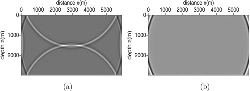
We now present two examples to show the numerical results of the forward problem. The first example is a homogeneous triangular model with constant velocity $3000\mathrm{m}/\mathrm{s}$ and constant density $1000{\mathrm{kg}/\mathrm{m}}^3$. The physical domain is $(x,z)=[0,6\mathrm{km}]\times [0,3\mathrm{km}]$. In computations, the spatial step is $h_x=h_z=12\mathrm{m}$ and the time step is $\mathrm{\Delta }t=0.001\mathrm{s}$. The source is located at $(3\mathrm{km},1.5\mathrm{km})$, which is the Ricker wavelet with the time history (76) $f(t)=(1-2(\pi f_{0}t{)}^2){\mathrm{e}}^{-(\pi f_{0}t{)}^2},$(76) where $f_0=15\mathrm{Hz}$ is the central frequency. Figure 1 is the snapshot of wavefield at propagation time $1.1\mathrm{s}$. Figure 1(a) is the result by the staggered-grid method without absorbing boundary conditions. In Figure 1(a), we can see the serious reflections from the top and bottom boundaries. Figure 1(b) is the result by the wavelet method with the PML boundary conditions. The PML is around the computational model. In Figure 1(b) we can see the boundary reflections are eliminated obviously.

Figure 1. The snapshot of wavefield at propagation time $1.1\mathrm{s}$ by the wavelet method (a) without absorbing boundary conditions and (b) with PML absorbing boundary conditions.

The second example is the Marmousi model [50] with complex structures. The exact velocity is shown in Figure 5 and it will be used in the inversion computations. The computational domain is $(x,z)=[0,6\mathrm{km}]\times [0,3\mathrm{km}]$. The spatial step is $h_x=h_z=12\mathrm{m}$ and the time step is $\mathrm{\Delta }t=0.001\mathrm{s}$. The thickness of PML is $420\mathrm{m}$. The shots and receivers are arranged under the surface $24\mathrm{m}$. The sketch map of the data acquisition system is shown in Figure 2. This data observation geometry is analogous to the acquisition system of reflection seismology in geophysical exploration. In Figure 2, the blue points denote the shots and the red crosses denote the receivers. Figure 3(a) is a shot gather with the shot located at the left side of the model. Figure 3(b) is another shot gather with the shot located at the middle of the model. In both Figure 3(a,b), we can see the boundary reflections are eliminated obviously. For comparison with Figure 3, the corresponding shot gather by the staggered-grid method is shown in Figure 4. Comparing Figure 4 with Figure 3, we can clearly see that the waveform in Figure 3 by the wavelet method has much less dispersion.

Figure 2. The sketch map of data acquisition system. The blue points denote the shots and the red crosses denote the receivers. The shots and receivers are arranged under the surface $24\mathrm{m}$. The thickness of PML is $420\mathrm{m}$.

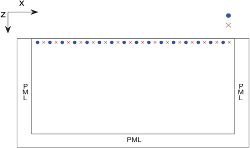
Figure 3. The shot gather for the Marmousi model computed by the wavelet method. The shot located at two different positions near the surface, i.e. (a) the left side of the model, x = 0; (b) the middle of the model, x = 3 km. Each shot has 200 receivers. The horizontal axis is the receiver points. The vertical axis is the time points.

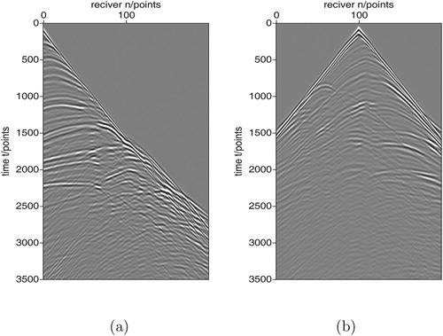
Figure 4. The shot gather for the Marmousi model computed by the staggered-grid method. The shot located at two different positions near the surface, i.e. (a) the left side of the model, x = 0; (b) the middle of the model, $x=3\mathrm{km}$. Each shot has 200 receivers. The horizontal axis is the receiver points. The vertical axis is the time points.

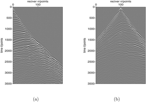
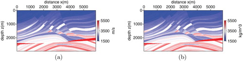
Figure 5. The Marmousi exact model. (a) velocity, (b) density.

4.2. Inversion computations

We now consider the FWI for the Marmousi model. This model is a benchmark model which is usually applied to test the ability of an inversion method. The exact model of velocity and density for the Marmousi model is shown in Figure 5. The density shown in Figure 5(b) varies from $1.5{\mathrm{g}/\mathrm{cm}}^3$ to $5.5{\mathrm{g}/\mathrm{cm}}^3$. The density structure is similar with the velocity because high velocity corresponds to large density physically. The data acquisition system is shown in Figure 2. The number of sampling points in space is $N_x=493$ and $N_z=249$ with the step $h_x=h_z=12\mathrm{m}$. The number of time points is $N_t=3501$ with the step $\mathrm{\Delta }t=0.001\mathrm{s}$. There are 80 shots and each shot 40 receivers totally. The space of receivers is $24\mathrm{m}$ and the space of shots is $48\mathrm{m}$. The initial model for FWI is shown in Figure 6, which is built by a linear increasing function from the surface to the bottom. Figure 6(a) is the initial velocity model and Figure 6(b) is the initial density model. As we can see, the initial model is quite different from the exact model and we can not see the useful information of complex structures such as the faults in the exact model Figure 5. The frequency multiscale strategy is applied in FWI. Particularly, we implement FWI from low frequency to high frequency step by step. And the inversion result at current frequency band is served as the initial model for the next frequency band. 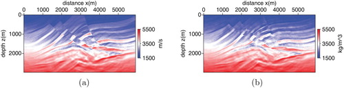In order to obtain the data in a certain frequency band, we apply the following Blackman-Harris window to filter the data: $w(n)=c_1+c_2\cos \left(\frac{2\pi n}{N_L}\right)+c_3\cos \left(\frac{4\pi n}{N_L}\right)+c_4\cos \left(\frac{6\pi n}{N_L}\right),$ where $N_L=500$ is the length of the filter and $c_1=0.35875,c_2=-0.48829,c_3=0.14128,c_4=-\mathrm{0.01168.}$ In computations, we set four different frequency bands. Moreover, the data in the current frequency band is contained the data in the next frequency band so the FWI is more robust. Figure 7 is the inversion result of velocity and density with the data from frequency 0 to 5 Hz. Figure 8 is the inversion result with the data from frequency 0 to 15 Hz. Figure 9 is the inversion result with the 0–25 Hz data. The iteration number is fifty. From Figures 7–9, we can see the inversion accuracy is improved gradually. Figure 10 is the final inversion result with the whole frequency band data. Comparing Figure 10 with Figure 5, we can see most of the structures of the exact model are inverted accurately.

Figure 6. The initial model for FWI. (a) velocity, (b) density.

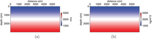
Figure 7. The inversion result with the 0–5 Hz data. (a) velocity, (b) density.

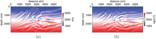
Figure 8. The inversion result with the 0–15 Hz data. (a) velocity, (b) density.

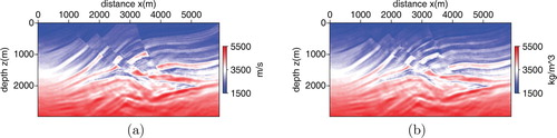
Figure 9. The inversion result with the 0–25 Hz data. (a) velocity, (b) density.

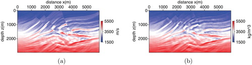
Figure 10. The inversion result with the whole frequency band data. (a) velocity, (b) density.

FWI is a typical large-scale computational problem. We implement the parallel computations based on the message passing interface (MPI). The physical domain is separated into different subdomains. And each subdomain is assigned to a different processer. The data exchanges only occur at the boundary of subdomains. In the L-BFGS algorithm, the computations for searching direction only involve vector inner product in a matrix-free fashion and the computations do not repeat in the overlapping area. The number of discretized parameters in inversion is 245,514. The CPU time for the whole FWI is about 14 h with 128 processes. The processor is the 3.6 GHz Intel. The stoping criteria for the inversion is when the $\Vert \mathrm{\nabla }\mathcal{F}(\mathit{m})\Vert$ is less than a small quantity while the iteration times are not beyond a fixed number.

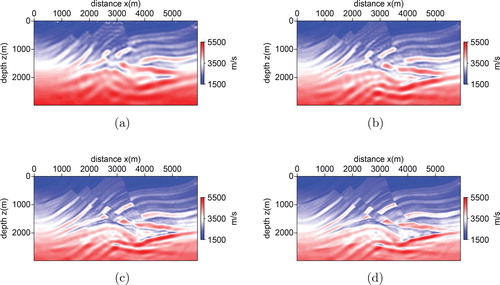
We remark that the multi-parameter FWI including the density is harder than the single parameter FWI because of the coupling influence between the density and velocity. The single parameter inversion has better accuracy than the multi-parameter inversion. Figure 11 shows the results of the single parameter inversion for velocity only by the wavelet method with the data in four different frequency bands, i.e. 0–2.5 Hz, 0–5 Hz, 0–15 Hz and all frequencies. From Figure 11(a,d), we can clearly see that the inversion accuracy improves gradually. Comparing Figure 11(a) with Figure 10(a), we also see that the final single parameter inversion result is better than the multi-parameter inversion, which is as we expected. In the computations, the observed data has been added the $5\mathrm{\%}$ Gaussian noises.

Figure 11. The single parameter inversion for velocity with the data in four different frequency bands. (a) 0–2.5 Hz, (b) 0–5 Hz, (c) 0–15 Hz, (d) all frequencies.

5. Conclusions

The FWI is an attractive tool to obtain high resolution subsurface parameters in complex geological structures. We have investigated the wavelet-based FWI for determining the density and velocity coefficients in the acoustic wave equation. The numerical methods and schemes are established. The method solves the forward problem by applying Daubechies-4 wavelet to approximate the wavefield on staggered grids. The discrete schemes for forward modelling and the corresponding stability condition are derived in detail. The inverse problem is solved iteratively by minimizing the waveform misfit between the synthetic data and the observed wafefield. The discrete schemes for the gradient are derived based on the matrix technique. The frequency multiscale method implements FWI from low frequency to high frequency successively. Moreover, the inversion result of current frequency band is served as the initial guesses of the next frequency band, which improves robustness and accuracy of FWI. The multi-parameter FWI with density has lower inversion accuracy than the single parameter inversion. In FWI computations, the initial model is far from the exact model, which shows the method is less dependent on the initial model. Numerical computations for a benchmark model show the effectiveness and robustness of the method in this paper. The method can be extended to elastic model FWI.

Acknowledgements

I appreciate J. Jiang for his valuable helps in this research. Thanks also give to the reviewers and the editor for their helps.

Disclosure statement

No potential conflict of interest was reported by the author(s).

Additional information

Funding

This research is supported by the National Natural Science Foundation of China under the grant numbers 11471328 and 51739007.

Appendices

Appendix 1. The computations for coefficients $r_{l+\frac{1}{2},i}$ in (40).

By the definition of (26(26) $\begin{array}{rl}{r}_{l+\frac{1}{2},i}^1& ={\int }_{-\mathrm{\infty }}^{+\mathrm{\infty }}\frac{\mathrm{\partial }\varphi (x-l-\frac{1}{2})}{\mathrm{\partial }x}\varphi (x-i)\mathrm{d}x,\end{array}$(26) ), we know (A1) $r_{l+\frac{1}{2},i}^1={\int }_{-\mathrm{\infty }}^{+\mathrm{\infty }}\varphi (x-i)\frac{\mathrm{\partial }\varphi (x-l-\frac{1}{2})}{\mathrm{\partial }x}\mathrm{d}x.$(A1) For brevity, we set ${\hat{r}}_{i-l-\frac{1}{2}}:=r_{l+\frac{1}{2},i}^1$. Then we can rewrite (A1(A1) $r_{l+\frac{1}{2},i}^1={\int }_{-\mathrm{\infty }}^{+\mathrm{\infty }}\varphi (x-i)\frac{\mathrm{\partial }\varphi (x-l-\frac{1}{2})}{\mathrm{\partial }x}\mathrm{d}x.$(A1) ) as (A2) ${\hat{r}}_{i-l-\frac{1}{2}}={\int }_{-\mathrm{\infty }}^{+\mathrm{\infty }}\varphi (x-i+l+\frac{1}{2})\frac{\mathrm{\partial }\varphi (x)}{\mathrm{\partial }x}\mathrm{d}x,$(A2) and by (11(11) $\begin{array}{rl}\varphi (x)& =\sqrt{2}\sum _{k=0}^{L-1}{h}_k\varphi (2x-k),\end{array}$(11) ) we have (A3) $\begin{array}{rl}{\hat{r}}_{i-l-\frac{1}{2}}& =4\sum _{k=0}^{L-1}\sum _{m=0}^{L-1}{h}_k{h}_m{\int }_{-\mathrm{\infty }}^{+\mathrm{\infty }}\varphi (2x-2i+2l+1-k){\varphi }^{\prime }(2x-m)\mathrm{d}x\\ & =2\sum _{k=0}^{L-1}\sum _{m=0}^{L-1}{h}_k{h}_m{\hat{r}}_{2i+k-2l-1-m}.\end{array}$(A3) Substituting m = k−n, we rewrite (A3(A3) $\begin{array}{rl}{\hat{r}}_{i-l-\frac{1}{2}}& =4\sum _{k=0}^{L-1}\sum _{m=0}^{L-1}{h}_k{h}_m{\int }_{-\mathrm{\infty }}^{+\mathrm{\infty }}\varphi (2x-2i+2l+1-k){\varphi }^{\prime }(2x-m)\mathrm{d}x\\ & =2\sum _{k=0}^{L-1}\sum _{m=0}^{L-1}{h}_k{h}_m{\hat{r}}_{2i+k-2l-1-m}.\end{array}$(A3) ) as (A4) $\begin{array}{rl}{\hat{r}}_{i-l-\frac{1}{2}}& =2\sum _{k=0}^{L-1}\sum _{n=k}^{k-L+1}{h}_k{h}_{k-n}{\hat{r}}_{2i+n-2l-1}\\ & =2\{\sum _{n=1-L}^{-1}\sum _{k=0}^{L-1+n}+\sum _{n=0}^{L-1}\sum _{k=n}^{L-1}\}{h}_k{h}_{k-n}{\hat{r}}_{2i+n-2l-1}\\ & =2\sum _{n=1}^{L-1}\sum _{k=0}^{L-1-n}{h}_k{h}_{k+n}{\hat{r}}_{2i-n-2l-1}+2\sum _{n=0}^{L-1}\sum _{k=0}^{L-1-n}{h}_k{h}_{k+n}{\hat{r}}_{2i+n-2l-1}\\ & =2\sum _{n=1}^{L-1}\sum _{k=0}^{L-1-n}{h}_k{h}_{k+n}({\hat{r}}_{2i-n-2l-1}+{\hat{r}}_{2i+n-2l-1})+2\sum _{k=0}^{L-1}{h}_k^2{\hat{r}}_{2i-2l-1}.\end{array}$(A4) Using the fact $\sum _{k=0}^{L-1}{h}_k^2=1$, we obtain (A5) ${\hat{r}}_{i-l-\frac{1}{2}}=2{\hat{r}}_{2i-2l-1}+\sum _{n=1}^{L-1}{a}_n({\hat{r}}_{2i-n-2l-1}+{\hat{r}}_{2i+n-2l-1}),$(A5) where $a_n$ are the autocorrelation coefficients of $h_k$ $(k=0,\dots ,L-1)$: (A6) $a_n=2\sum _{k=0}^{L-1-n}{h}_k{h}_{k+n},n=1,\dots ,L-1.$(A6) In fact, for Daubechies' wavelets with M vanishing moments, $a_n$ can be expressed as [51] $a_{2m-1}=\frac{(-1{)}^{m-1}{C}_M}{(M-m)!(M+m-1)!(2m-1)},m=1,\dots ,M,$ where $C_M={\left[\frac{(2M-1)!}{(M-1)!4^{M-1}}\right]}^2.$ Note that coefficients $a_n$ with even indices are zero. We remark ${\hat{r}}_i$ on integer grids $i\in \mathbb{Z}$ can be computed by solving a linear system. For example, for the Daubechies wavelet with M = 4, we have $\begin{array}{rl}& {\hat{r}}_1=-7.9300952\mathrm{E}-01,{\hat{r}}_2=1.9199897\mathrm{E}-01,\\ & {\hat{r}}_3=-3.3580207\mathrm{E}-02,{\hat{r}}_4=2.2240497\mathrm{E}-03,\\ & {\hat{r}}_5=1.7220619\mathrm{E}-04,{\hat{r}}_6=-8.4085053\mathrm{E}-07.\end{array}$ So by (A5(A5) ${\hat{r}}_{i-l-\frac{1}{2}}=2{\hat{r}}_{2i-2l-1}+\sum _{n=1}^{L-1}{a}_n({\hat{r}}_{2i-n-2l-1}+{\hat{r}}_{2i+n-2l-1}),$(A5) ) and setting $i=l+1,\dots ,l+7$ we can obtain the results on staggered grids in (40(40) $\begin{array}{rl}& r_{l+\frac{1}{2},l+1}^1=-r_{l+\frac{1}{2},l}^1=-1.3110341,\\ & r_{l+\frac{1}{2},l+2}^1=-r_{l+\frac{1}{2},l-1}^1=1.5601008\mathrm{E}-01,\\ & r_{l+\frac{1}{2},l+3}^1=-r_{l+\frac{1}{2},l-2}^1=-4.1995747\mathrm{E}-02,\\ & r_{l+\frac{1}{2},l+4}^1=-r_{l+\frac{1}{2},l-3}^1=8.6543237\mathrm{E}-03,\\ & r_{l+\frac{1}{2},l+5}^1=-r_{l+\frac{1}{2},l-4}^1=-8.3086955\mathrm{E}-04,\\ & r_{l+\frac{1}{2},l+6}^1=-r_{l+\frac{1}{2},l-5}^1=-1.0899854\mathrm{E}-05,\\ & r_{l+\frac{1}{2},l+7}^1=-r_{l+\frac{1}{2},l-6}^1=4.1057155\mathrm{E}-09,\\ & r_{l+\frac{1}{2},l+q}^1=0,q<-6\mathrm{or}q>7.\end{array}$(40) ).

Appendix 2. The elements of matrix $\frac{\mathrm{\partial }M}{\mathrm{\partial }{v}_{i,j}}$ in (67) and the elements of matrix $\frac{\mathrm{\partial }M}{\mathrm{\partial }{\rho }_{i,j}}$ in (70).

The elements of matrix $\frac{\mathrm{\partial }M}{\mathrm{\partial }{v}_{i,j}}$ are $\frac{\mathrm{\partial }A}{\mathrm{\partial }{v}_{i,j}}$. By the expression of A in (59(59) $\begin{array}{rl}{\overline{u}}^n& ={(u_{0,0}^n,\dots ,u_{0,N_z}^n,\dots ,u_{N_x,0}^n,\dots ,u_{N_x,N_z}^n)}^T,\\ {\overline{f}}^n& ={(f_{0,0}^n,\dots ,f_{0,N_z}^n,\dots ,f_{N_x,0}^n,\dots ,f_{N_x,N_z}^n)}^T,\\ A& =\frac{1}{\mathrm{\Delta }{t}^2}\left(\begin{array}{cccc}{\displaystyle \frac{1}{\rho v_{0,0}^2}}& 0& \cdots & 0\\ 0& {\displaystyle \frac{1}{\rho v_{0,1}^2}}& \cdots & 0\\ ⋮& ⋮& \ddots & ⋮\\ 0& 0& \cdots & {\displaystyle \frac{1}{\rho v_{N_x,N_z}^2}}\end{array}\right),\end{array}$(59) ), we have (A7) $\frac{\mathrm{\partial }A}{\mathrm{\partial }{v}_{i,j}}=\frac{1}{\mathrm{\Delta }{t}^2}\left(\begin{array}{ccccc}0& 0& \cdots & 0& 0\\ 0& \ddots & 0& 0& 0\\ ⋮& 0& -{\displaystyle \frac{2}{\rho v_{i,j}^3}}& 0& ⋮\\ 0& 0& 0& \ddots & 0\\ 0& 0& \cdots & 0& 0\end{array}\right).$(A7) Note that $\frac{\mathrm{\partial }K}{\mathrm{\partial }{v}_{i,j}}=\mathbf{0}$.

The elements of matrix $\frac{\mathrm{\partial }M}{\mathrm{\partial }{\rho }_{i,j}}$ in (70(70) $\frac{\mathrm{\partial }M}{\mathrm{\partial }{\rho }_{i,j}}=\left(\begin{array}{ccccc}{\displaystyle \frac{\mathrm{\partial }A}{\mathrm{\partial }{\rho }_{i,j}}}& 0& 0& \cdots & 0\\ -2{\displaystyle \frac{\mathrm{\partial }A}{\mathrm{\partial }{\rho }_{i,j}}}-{\displaystyle \frac{\mathrm{\partial }K}{\mathrm{\partial }{\rho }_{i,j}}}& {\displaystyle \frac{\mathrm{\partial }A}{\mathrm{\partial }{\rho }_{i,j}}}& 0& \cdots & 0\\ {\displaystyle \frac{\mathrm{\partial }A}{\mathrm{\partial }{\rho }_{i,j}}}& -2{\displaystyle \frac{\mathrm{\partial }A}{\mathrm{\partial }{\rho }_{i,j}}}-{\displaystyle \frac{\mathrm{\partial }K}{\mathrm{\partial }{\rho }_{i,j}}}& {\displaystyle \frac{\mathrm{\partial }A}{\mathrm{\partial }{\rho }_{i,j}}}& \cdots & 0\\ ⋮& \ddots & \ddots & \ddots & 0\\ 0& \cdots & {\displaystyle \frac{\mathrm{\partial }A}{\mathrm{\partial }{\rho }_{i,j}}}& -2{\displaystyle \frac{\mathrm{\partial }A}{\mathrm{\partial }{\rho }_{i,j}}}-{\displaystyle \frac{\mathrm{\partial }K}{\mathrm{\partial }{\rho }_{i,j}}}& {\displaystyle \frac{\mathrm{\partial }A}{\mathrm{\partial }{\rho }_{i,j}}}\end{array}\right),$(70) ) are $\frac{\mathrm{\partial }A}{\mathrm{\partial }{\rho }_{i,j}}$ and $\frac{\mathrm{\partial }K}{\mathrm{\partial }{\rho }_{i,j}}$. By the expression of A in (59(59) $\begin{array}{rl}{\overline{u}}^n& ={(u_{0,0}^n,\dots ,u_{0,N_z}^n,\dots ,u_{N_x,0}^n,\dots ,u_{N_x,N_z}^n)}^T,\\ {\overline{f}}^n& ={(f_{0,0}^n,\dots ,f_{0,N_z}^n,\dots ,f_{N_x,0}^n,\dots ,f_{N_x,N_z}^n)}^T,\\ A& =\frac{1}{\mathrm{\Delta }{t}^2}\left(\begin{array}{cccc}{\displaystyle \frac{1}{\rho v_{0,0}^2}}& 0& \cdots & 0\\ 0& {\displaystyle \frac{1}{\rho v_{0,1}^2}}& \cdots & 0\\ ⋮& ⋮& \ddots & ⋮\\ 0& 0& \cdots & {\displaystyle \frac{1}{\rho v_{N_x,N_z}^2}}\end{array}\right),\end{array}$(59) ), we have (A8) $\frac{\mathrm{\partial }A}{\mathrm{\partial }{\rho }_{i,j}}=\frac{1}{\mathrm{\Delta }{t}^2}\left(\begin{array}{ccccc}0& 0& \cdots & 0& 0\\ 0& \ddots & 0& 0& 0\\ ⋮& 0& -{\displaystyle \frac{1}{(\rho v_{i,j}{)}^2}}& 0& ⋮\\ 0& 0& 0& \ddots & 0\\ 0& 0& \cdots & 0& 0\end{array}\right).$(A8) And by the expression of K in (60(60) $\begin{array}{rl}K& =\left(\begin{array}{cccc}{K}_{0,0}& K_{1,0}& \cdots & 0\\ K_{0,1}& K_{1,1}& K_{2,1}& 0\\ ⋮& \ddots & \ddots & ⋮\\ 0& \cdots & K_{N_x,N_x-1}& K_{N_x,N_x}\end{array}\right),\end{array}$(60) ), we have (A9) $\frac{\mathrm{\partial }K}{\mathrm{\partial }{\rho }_{i,j}}=\left(\begin{array}{ccccc}{\displaystyle \frac{\mathrm{\partial }{K}_{0,0}}{\mathrm{\partial }{\rho }_{i,j}}}& {\displaystyle \frac{\mathrm{\partial }{K}_{1,0}}{\mathrm{\partial }{\rho }_{i,j}}}& \cdots & 0& 0\\ {\displaystyle \frac{\mathrm{\partial }{K}_{0,1}}{\mathrm{\partial }{\rho }_{i,j}}}& {\displaystyle \frac{\mathrm{\partial }{K}_{1,1}}{\mathrm{\partial }{\rho }_{i,j}}}& {\displaystyle \frac{\mathrm{\partial }{K}_{2,1}}{\mathrm{\partial }{\rho }_{i,j}}}& 0& 0\\ ⋮& \ddots & \ddots & \ddots & ⋮\\ 0& 0& {\displaystyle \frac{\mathrm{\partial }{K}_{N_x-2,N_x-1}}{\mathrm{\partial }{\rho }_{i,j}}}& {\displaystyle \frac{\mathrm{\partial }{K}_{N_x-1,N_x-1}}{\mathrm{\partial }{\rho }_{i,j}}}& {\displaystyle \frac{\mathrm{\partial }{K}_{N_x,N_x-1}}{\mathrm{\partial }{\rho }_{i,j}}}\\ 0& 0& \cdots & {\displaystyle \frac{\mathrm{\partial }{K}_{N_x-1,N_x}}{\mathrm{\partial }{\rho }_{i,j}}}& {\displaystyle \frac{\mathrm{\partial }{K}_{N_x,N_x}}{\mathrm{\partial }{\rho }_{i,j}}}\end{array}\right),$(A9) where $\begin{array}{rl}& \frac{\mathrm{\partial }{K}_{i+1,i}}{\mathrm{\partial }{\rho }_{i,j}}=\frac{\mathrm{\partial }{K}_{i,i-1}}{\mathrm{\partial }{\rho }_{i,j}}=\frac{\mathrm{\partial }{K}_{i,i+1}}{\mathrm{\partial }{\rho }_{i,j}}=\frac{\mathrm{\partial }{K}_{i-1,i}}{\mathrm{\partial }{\rho }_{i,j}}=\left(\begin{array}{ccccc}0& 0& \cdots & 0& 0\\ 0& \ddots & 0& 0& 0\\ ⋮& 0& -{\displaystyle \frac{1}{2{\rho }_{i,j}^2}}{\displaystyle \frac{1}{h_x^2}}& 0& ⋮\\ 0& 0& 0& \ddots & 0\\ 0& 0& \cdots & 0& 0\end{array}\right),\\ & \frac{\mathrm{\partial }{K}_{s+1,s}}{\mathrm{\partial }{\rho }_{i,j}}=\mathbf{0},\frac{\mathrm{\partial }{K}_{s,s+1}}{\mathrm{\partial }{\rho }_{i,j}}=\mathbf{0},s\ne i-1,i,\\ & \frac{\mathrm{\partial }{K}_{i,i}}{\mathrm{\partial }{\rho }_{i,j}}=\left(\begin{array}{ccccccc}0& 0& 0& \cdots & 0& 0& 0\\ 0& \ddots & 0& \cdots & 0& 0& 0\\ 0& 0& {\displaystyle \frac{1}{2{\rho }_{i,j}^2}}{\displaystyle \frac{1}{h_z^2}}& -{\displaystyle \frac{1}{2{\rho }_{i,j}^2}}{\displaystyle \frac{1}{h_z^2}}& 0& 0& 0\\ ⋮& ⋮& -{\displaystyle \frac{1}{2{\rho }_{i,j}^2}}{\displaystyle \frac{1}{h_z^2}}& {\displaystyle \frac{1}{{\rho }_{i,j}^2}}({\displaystyle \frac{1}{h_z^2}}+{\displaystyle \frac{1}{h_x^2}})& -{\displaystyle \frac{1}{2{\rho }_{i,j}^2}}{\displaystyle \frac{1}{h_z^2}}& ⋮& ⋮\\ 0& 0& 0& -{\displaystyle \frac{1}{2{\rho }_{i,j}^2}}{\displaystyle \frac{1}{h_z^2}}& {\displaystyle \frac{1}{2{\rho }_{i,j}^2}}{\displaystyle \frac{1}{h_z^2}}& 0& 0\\ 0& 0& 0& \cdots & 0& \ddots & 0\\ 0& 0& 0& \cdots & 0& 0& 0\end{array}\right),\\ & \frac{\mathrm{\partial }{K}_{i\pm 1,i\pm 1}}{\mathrm{\partial }{\rho }_{i,j}}=\left(\begin{array}{ccccc}0& 0& \cdots & 0& 0\\ 0& \ddots & 0& 0& 0\\ ⋮& 0& {\displaystyle \frac{1}{2{\rho }_{i,j}^2}}{\displaystyle \frac{1}{h_x^2}}& 0& ⋮\\ 0& 0& 0& \ddots & 0\\ 0& 0& \cdots & 0& 0\end{array}\right),\frac{\mathrm{\partial }{K}_{s,s}}{\mathrm{\partial }{\rho }_{i,j}}=\mathbf{0},s\ne i,i\pm 1.\end{array}$

References

- Lailly P. The seismic inverse problem as a sequence of before stack migrations. Conference on Inverse Scattering, Theory and Applications. Philadelphia (PA): SIAM; 1983. p. 206–220.
- Tarantola A. Inversion of seismic reflection data in the acoustic approximation. Geophysics. 1984;49(8):1259–1266.
- Mora P. Nonlinear two-dimensional elastic inversion of multioffset seismic data. Geophysics. 1987;52(9):1211–1228.
- Tarantola A. A strategy for nonlinear elastic inversion of seismic reflection data. Geophysics. 1986;51(10):1893–1903.
- Pratt RG, Worthington MH. Inverse theory applied to multi-source cross-hole tomography, part 1: acoustic wave equation method. Geophys Prospect. 1990;38(3):287–310.
- Pratt RG. Inverse theory applied to multi-source cross-hole tomography, part 2: elastic wave equation method. Geophys Prospect. 1990;38(3):311–329.
- Virieux J, Operto S. An overview of full-waveform inversion in exploration geophysics. Geophysics. 2009;74(6):WCC1–WCC26.
- Shin C, Cha YH. Waveform inversion in the Laplace-Fourier domain. Geophys J Int. 2009;177(3):1067–1079.
- Shin C, Cha YH. Waveform inversion in the Laplace domain. Geophys J Int. 2008;173(3):922–931.
- Yang P, Brossier R, Métivier L, et al. A time-domain preconditioned truncated Newton approach to viso-acoostic multiparameter full waveform inversion. SIAM J Sci Comput. 2018;40(4):B1101–B1130.
- Aghamiry HS, Gholami A, Operto S. ADMM-based multi-parameter wavefield reconstruction inversion in VTI acoustic media with TV regularization. Geophys J Int. 2019;219(2):1316–1333.
- Métivier L, Brossier R, Operto S, et al. Full waveform inversion and the truncated Newton method. SIAM Rev. 2017;59(1):153–195.
- Plessix RE. A review of the adjoint-state method for computing the gradient of a functional with geophysical applications. Geophys J Int. 2006;167(2):495–503.
- Pratt RG, Shin C, Hicks GJ. Gauss-Newton and full Newton methods in frequency-space seismic waveform inversion. Geophys J Internat. 1998;133(2):341–362.
- Epanomeritakis I, Akelik V, Ghattas O, et al. A Newton-CG method for large-scale three-dimensional elastic full waveform seismic inversion. Inverse Problems. 2008;24(3):1–26.
- Engl H, Hanke M, Neubauer A. Regularization of inverse problems. Dordrecht: Kluwer Academic Publishers Group; 1996.
- Guitton A. Blocky regularization schemes for full-waveform inversion. Geophys Prospect. 2012;60(5):870–884.
- Lin Y, Huang L. Acoustic- and elastic-waveform inversion using a modified total-variation regularization scheme. Geophys J Int. 2015;200(1):489–502.
- Bunks C, Saleck F, Zaleski S, et al. Multiscale seismic waveform inversion. Geophysics. 1995;60(5):1457–1473.
- Engquist E, Froese BD. Application of the Wasserstein metric to seismic signals. Commun Math Sci. 2014;12(5):979–988.
- Métivier L, Brossier R, Mérigot Q, et al. Measuring the misfit between seismograms using an optimal transport distance: application to full waveform inversion. Geophys J Int. 2016;205(1):345–377.
- Virieux J. P-SV wave propagation in heterogeneous media: velocity-stress finite-difference method. Geophysics. 1986;51(4):889–901.
- Zhang W, Tong L, Chung ET. A new high accuracy locally one-dimensional scheme for the wave equation. J Comput Appl Math. 2011;236(6):1343–1353.
- Fornberg B. A practical guide to pseudospectral methods. Cambridge: Cambridge University Press; 1996.
- Zhang W. Stability conditions for wave simulation in 3-D anisotropic media with the pseudospectral method. Commun Comput Phys. 2012;12(3):703–720.
- Zhang W, Zhuang Y, Zhang L. A new high-order finite volume method for 3D elastic wave simulation on unstructured meshes. J Comput Phys. 2017;340:534–555.
- Cohen G. Higher-order numerical methods for transient wave equations. Berlin: Springer-Verlag; 2002.
- Zhang W, Chung ET, Wang C. Stability for imposing absorbing boundary conditions in the finite element simulation of acoustic wave propagation. J Comput Math. 2014;32(1):1–20.
- Zhang W. Elastic full waveform inversion on unstructured meshes by the finite element method. Phys Scr. 2019;94: 115002.
- Beylkin G, Keiser JM. On the adaptive numerical solution of nonlinear partial differential equations in wavelet bases. J Comput Phys. 1997;132(2):233–259.
- Dahmen W. Wavelet and multiscale methods for operator equations. Acta Numer. 1997;6:55–228.
- Fröhlich J, Schneider K. An adaptive wavelet-vaguelette algorithm for the solution of PDEs. J Comput Phys. 1997;130(2):174–190.
- Hong TK, Kennett BLN. On a wavelet-based method for the numerical simulation of wave propagation. J Comput Phys. 2002;183(2):577–622.
- Qian S, Weiss J. Wavelets and the numerical solution of partial differential equations. J Comput Phys. 1993;106(1):155–175.
- Lions LJ, Magenes E. Non-homogeneous boundary value problems and application. Vol. 1. New York (NY): Springer-Verlag; 1972.
- Chui C. Wavelets: a tutorial in theory and applications. San Diego (CA): Academic Press; 1992.
- Daubechies I. Orthonormal bases of compactly supported wavelets. Commun Pure Appl Math. 1988;41:901–906.
- Daubechies I. Ten lectures on wavelet. Philadelphia (PA): Society for Industrial and Applied Mathematics; 1992.
- Mallat S. Multiresolution approximations and wavelet orthogonal bases of L2(R). Trans Amer Math Soc. 1989;315:69–88.
- Clayton R, Engquist B. Absorbing boundary conditions for acoustic and elastic wave equations. Bull Seismol Soc Am. 1977;67(6):1529–1540.
- Grote MJ, Keller JB. Exact nonreflecting boundary condition for elastic waves. SIAM J Appl Math. 2000;60(3):803–819.
- Zhang W, Tong L, Chung ET. Exact nonreflecting boundary conditions for three dimensional poroelastic wave equations. Commun Math Sci. 2014;12(1):61–98.
- Berenger JP. A perfectly matched layer for the absorption of electromagnetic waves. J Comput Phys. 1994;114(2):185–200.
- Thomas JW. Numerical partial differential equations: finite difference methods. New York (NY): Springer Science Business Media; 1995.
- Nocedal J, Wright ST. Numerical optimization. New York (NY): Springer Science Business Media; 1990.
- Dembo RS, Steihaug T. Truncated Newton algorithms for large-scale unconstrained optimization. Math Program. 1983;26(2):190–212.
- Klibanov MV. Global convexity in a three-dimensional inverse acoustic problem. SIAM J Math Anal. 1997;28(6):1371–1388.
- Khoa VA, Klibanov MV, Nguyen LH. Convexification for a three-dimensional inverse scattering problem with the moving point source. SIAM J Imaging Sci. 2020;13(2):871–904.
- Klibanov MV, Kolesov AE, Nguyen LH. Convexification method for an inverse scattering problem and its performance for experimental backscatter data fir buried targets. SIAM J Imaging Sci. 2019;12(1):576–603.
- Martin GS, Wiley R, Marfurt KJ. Marmousi2: an elastic upgrade for Marmousi. Leading Edge. 2006;25:156–166.
- Beylkin G. On the representation of operators in bases of compactly supported wavelet. SIAM J Numer Anal. 1992;29(6):1716–1740.
Appendices
Appendix 1. The computations for coefficients  in (40).
By the definition of (Equation26(26)
(26) ), we know
(A1)
(A1) For brevity, we set
. Then we can rewrite (EquationA1
(A1) ) as
(A2)
(A2) and by (Equation11
(11)
(11) ) we have
(A3)
Substituting m = k−n, we rewrite (EquationA3
(A3) ) as
(A4)
Using the fact
, we obtain
(A5)
(A5) where
are the autocorrelation coefficients of
:
(A6)
(A6) In fact, for Daubechies' wavelets with M vanishing moments,
can be expressed as [Citation51]
where
Note that coefficients
with even indices are zero. We remark
on integer grids
can be computed by solving a linear system. For example, for the Daubechies wavelet with M = 4, we have
So by (EquationA5
(A5) ) and setting
we can obtain the results on staggered grids in (Equation40
(40)
(40) ).
Appendix 2. The elements of matrix in (67) and the elements of matrix in (70).
The elements of matrix are
. By the expression of A in (Equation59
(59)
(59) ), we have
(A7)
(A7) Note that
.
The elements of matrix in (Equation70
(70)
(70) ) are
and
(A8)
(A8) And by the expression of K in (Equation60