Inverse problem solving in semiconductor photoacoustics by neural networks

Abstract

We developed a method of inverse problem solving in semiconductor photoacoustics based on neural networks application. Simple structured neural networks, trained on a large set of data obtained by the well – known theoretical models in the 20 Hz–20 kHz modulation frequency range, are applied to determine thermal diffusivity, coefficient of linear expansion and thickness of n – type silicon samples, using undistorted experimental photoacoustic signals. The efficiency of the neural networks was tested depending on the type of input data, showing the best performances in the case when signal amplitudes and phases are simultaneously presented to the network. Real – time parameter prediction is achieved together with high accuracy and reliability allowing one to perform the full characterization of a sample in the frequency domain.

KEYWORDS:

• Semiconductors
• photothermal
• photoacoustic
• thermal distribution
• artificial neural networks
• experimental signal
• inverse problem
• n – type silicon

2010 MATHEMATICS SUBJECT CLASSIFICATIONS:

• 536.2.01
• 536.21
• 004.032.26
• 544.527.5

1. Introduction

The characteristics of semiconductor samples can be determined by measuring their photoacoustic (PA) response in the 20 Hz–20 kHz frequency domain, generated by the sample illumination using a modulated light source and an open photoacoustic cell (OPC) experimental set – up [1,2]. Investigating the PA response, a number of theoretical models that allow an accurate interpretation of measured signals have been developed [3,4]. Based on a good match between the theory and experiment, together with a correct choice of data processing methods, thermal and mechanical parameters of a semiconductor sample can be reliably and accurately obtained, allowing its detailed characterization in terms of thermal diffusion (TD), thermoelastic (TE) and plasmaelastic (PE) effects [5–10].

In recent years, artificial neural networks (ANNs) have been used in physics as a very important tool for data processing. Most often ANNs have been trained on experimental data, and then used for a precise prediction of the tested sample characteristics [9–11]. However, such an approach is not recommended in PA measurements, because noise, distortion, and interference often mask the ‘true’ PA signal, mostly due to the instrumental response (detectors, amplifiers, modulators …) in frequency domain [12,13]. The prediction of networks trained on distorted experimental signals would not be accurate without the knowledge about the instrumental characteristics. Based on our experience within the pulsed photoacoustics of gases [14,15] and semiconductors [16], a better approach to the ANN training process should be to use a large set of undistorted signals generated by a well – known theoretical model adapted to the existing experimental conditions. Furthermore, for independent ANN test, PA experimental signals should be introduced to the network, rectified in such a way that their degree of distortion is assumed to be a well – known function of the preset instrumental features.

This paper presents an idea of the inverse problem solving in semiconductor photoacoustics using ANNs trained with undistorted signals which are obtained using well – known 1D theoretical models [3–6,17,18]. Briefly, the rectified PA experimental signals (amplitudes and phases) from the n-type silicon plates (thickness of 830, 417 and 128 µm) are introduced to different ANNs in order to obtain reliable, accurate and precise values of the investigated sample physical parameters (thermal diffusivity, thermal expansion, and thickness) in real – time. These parameters are used to calculate the causal effects (thermal diffusion, thermoelastic and plasmaelastic) that produce such signals. Performing the calculation in the whole PA frequency range of 20 Hz–20 kHz, adopted for OPC experimental set – up, the full characterization of semiconductor is achieved; the inverse problem is solved.

The use of different ANNs in our case means that the same network structure is used (one input, one hidden and one output layer) but with various input data: (a) amplitudes and phases; (b) only amplitudes; (c) only phases of the PA signals. The focus of our analysis was to show that only when ANNs are trained simultaneously with both amplitudes and phases of the PA signals in the frequency domain, the required precision, accuracy, and reliability in the parameter prediction could be achieved, enabling one to perform full characterization of the tested samples in real-time.

2. Theoretical background

2.1. Photoacoustic response of semiconductors

Photoacoustic signals in a semiconductor sample are mostly generated as a consequence of its thermal state changes due to the light–matter interaction during the sample illumination with a modulated light source, having the intensity $I=I_0\mathrm{Re}(1+e^{i\omega t})$, where $\omega =2\pi f$, $f$ is the light modulation frequency and $I_0$ is the incident light amplitude. Thermal state changes are followed by the heat transport within the sample accompanied by TD and TE effects. Beside thermal state changes, light–matter interaction in semiconductors could generate free carriers, significantly changing the concentration of minority ones. This effect of carrier generation depends on the light source wavelength and contributes to the heat transport in the semiconductor, too, changing the temperature distribution both at the surfaces and in the bulk, as well as the intensity of TD and TE effects. Carrier generation could also generate mechanical stress in the sample followed by PE effects [19–24].

The photoacoustic response of semiconductors is a combination of TD, TE and PE effects. It could be explained using the model of a composite piston: thermal (t) and mechanical (m) one. This is the reason why the total PA signal $\delta p_{\text{total}}(f)$ in the most general form can be written as a combination of thermal $\delta p_{\text{t}}(f)$ and mechanical $\delta p_{\text{m}}(f)$ components [4–6]: (1) $\delta p_{\text{total}}(f)=\delta p_{\text{t}}(f)+\delta p_{\text{m}}(f).$(1) here, the $\delta p_{\text{t}}(f)$ component represents a periodic pressure wave originating from the thermal piston existence. It is explained as a periodic expansion of the gas layer near the semiconductor non – illuminated surface due to surface periodic temperature changes. Such changes are determined by TD effects so in all our further notation we will take that $\delta p_{\text{t}}(f)=\delta p_{\text{TD}}(f)$. On the other hand, the $\delta p_{\text{m}}(f)$ component represents a periodic pressure wave originating from the mechanical piston existence. It is explained as a periodic compression of the air behind the non – illuminated semiconductor surface due to the sample bending, induced by two effects: (1) the TE effect (different temperatures at illuminated and non – illuminated sample surfaces) and (2) the PE effect (different minority carrier concentrations at illuminated and non-illuminated sample surfaces). This is the reason why we can write that $\delta p_{\text{m}}(f)=\delta p_{\text{TE}}(f)+\delta p_{\text{PE}}(f)$. Now, we can write the expression for $\delta p_{\text{total}}(f)$ (Equation (1)) in the form that can be usually found in the literature [19–24]: (2) $\delta p_{\text{total}}(f)=\delta p_{\text{TD}}(f)+\delta p_{\text{TE}}(f)+\delta p_{\text{PE}}(f).$(2) Our further analysis will account for the few assumptions: circular plates are used as samples having a cylindrical symmetry about the x – axis parallel to the surface normal to them; plate thicknesses are significantly lower than their radius; plates are irradiated uniformly. These assumptions allow us to reduce our analysis to 1D problem, neglecting lateral effects and using the simple theory of elastic thin plate to obtain its thermal and plasma elastic bending. Assuming 1D heat and carrier transfer processes, the expressions for the $\delta p_{\text{TD}}(f)$, $\delta p_{\text{TE}}(f)$ and $\delta p_{\text{PE}}(f)$ components could be given as [12,13,19]: (3) $\delta p_{\text{TD}}(f)=\frac{\gamma p_0\sqrt{D_g}}{l_c{T}_0\sqrt{\text{2}\pi if}}{T}_s(l,f),$(3) and (4) $\delta p_{\text{TE}}(f)={\alpha }_T\frac{\gamma p_0}{V_0}\frac{3\pi R_s^4}{l^3}{\int }_0^1\left(x-\frac{l}{2}\right)T_s(x,f)\text{d}x,$(4) (5) $\delta p_{\text{PE}}(f)=d_n\frac{\gamma p_0}{V_0}\frac{3\pi R_s^4}{l^3}{\int }_0^1\left(x-\frac{l}{2}\right)\delta n_p(x,f)\mathrm{d}x,$(5) where $D_g$ is the gas thermal diffusivity, $l_c$ is the photoacoustic cell length (the path from the sample to the microphone membrane), $\gamma$ is the adiabatic ratio, $p_0$, $T_0$ and$V_0$ are the pressure, temperature and volume of the photoacoustic cell, respectively, ${\alpha }_{\text{T}}$ is the thermal expansion coefficient, $l$ is the sample thickness, $R_s$ is the sample radius, $T_s(x,f)$ is the total temperature distribution in the sample [23,24], $T_s(l,f)$ is the temperature at the non-illuminated surface (x = l), $\delta n_p(x,f)$ is the minority carrier (in our case holes) concentration and $d_n$ is the coefficient of electronic deformation.$T_s(x,f)$ carries the information about the thermal diffusivity of the sample$D_{\text{T}}=k(\rho c_P{)}^{-1}$($k$ is the heat conductivity coefficient, $\rho$ is the density, $c_P$ is the specific heat) and the influence of minority carriers on heat distribution within the sample.

2.2. Signal correction procedure

The distortion of PA signals is an important question if experimental conditions and data collection process is considered. Our experience shows that there exist various sources of distortion: from different types of noises $N(f)$ to finite acoustic and electronic system response $H(f)$. All of them alter the $\delta p_{\text{total}}(f)$ signal amplitude $A_{\text{total}}(f)$ and phase ${\phi }_{\text{total}}(f)$ to different degrees across the whole 20 Hz–20 kHz modulation frequency range, especially at its endings [12,13,26]. Having a good signal-to-noise ratio $(N(f)<<S(f))$ the signal $S(f)$ recorded during the experiment can be written as [12,13,25]: (6) $S(f)=\delta p_{\text{total}}(f)H(f).$(6)

Following the signal correction procedure explained in details in [12,13,25] one can correct $S(f)$ removing all detected deviations $H(f)$ targeting $\delta p_{\text{total}}(f)$ (Equation (2)) in the form: (7) $\delta p_{\text{total}}(f)=A_{\text{total}}(f)\exp [i{\phi }_{\text{total}}(f)].$(7) here $\delta p_{\text{total}}(f)$ is also known as the so – called ‘true’ photoacoustic signal originating from the sample itself, clear of all possible instrumental and ambient influences.

2.3. Applied artificial neural networks

Generally speaking, artificial neural networks (ANNs) are a set of algorithms designed to recognize patterns or classify data. They are composed of a large number of interconnected processing elements (neurons) working together to solve specific problems. ANNs have the ability to derive meaning from randomly chosen data, extracting patterns and detecting trends that are usually hidden behind complex processes involved. They learn by example, trying to find correlations between inputs and outputs assuming that they are related at all [9–11].

It is a well – known fact that, in photoacoustics, there is a strong correlation between $A_{\text{total}}(f)$ and ${\phi }_{\text{total}}(f)$ shapes (patterns) in the frequency domain and sample characteristic parameters $D_{\text{T}}$, ${\alpha }_{\text{T}}$ and $l$. This was the basis for an idea to apply ANNs to recognize such shapes and find the mutual relationship between PA signal amplitudes and phases numerical values (curve values for corresponding frequencies) as inputs, and sample characteristic parameter values as an output. Based on our previous experience [14,16], the most useful ANN for these purposes is a Multilayer Layer Perceptron (MLP) network which consists of an input layer, several hidden layers, and an output layer. Its processing element – neuron is presented in Figure 1.

Figure 1. Typical presentation of an MLP network neuron.

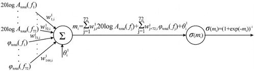
The inputs of the neuron in this case are $\delta p_{\text{total}}(f)$ signal amplitudes $A_{\text{total}}(f)$ and phases ${\phi }_{\text{total}}(f)$ (Equation (7)) defined in 72 equidistant frequency points each. The $A_{\text{total}}(f)$ changes in the given frequency range are usually in several magnitudes of order compared to ${\phi }_{\text{total}}(f)$ changes being in the range of a few hundred degrees. This is the reason why we normalize amplitudes with the simple function $20\log A_{\text{total}}(f)$, knowing that input data normalization, prior to a training process, is crucial to obtaining good results as well as to significantly speeding the calculations [16,26,27]. All neuron inputs are multiplied with weights $w_{n,i}^1$, where n is the number of the input and i is the number of neurons, and summed up together with the constant bias ${\theta }_i^1$. The resulting m_i (see Figure 1) is the input of the activation function, most commonly used as a sigmoid σ function: (8) $\sigma (m_i)=\frac{1}{1+\exp (-m_i)}.$(8) The value of the σ function is the neuron output.

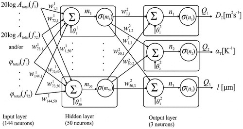
An ANN is formed by connecting multiple neurons, presented in Figure 1, in parallel and series. Being appropriate for the task, the network structure presented in Figure 2 is adopted in general, with one input layer (i = 144 neurons), one hidden layer (i = 50 neurons) and one output layer (i = 3 neurons). The number of neurons comprising input layer is equal to the number of frequency points in our data. Trying to simplify the network, relying on empirically-derived conclusions, the optimal number of hidden layer neurons is taken to be between the number of the input and number of the output neurons. The outputs Q_i of the output layer neurons corresponds to sample parameters $D_{\text{T}}$, ${\alpha }_{\text{T}}$ and $l$. For ANN training, the back propagation Levenberg – Marquardt algorithm was used, while the mean squared error (MSE) was used as a performance measure during training [27].

Figure 2. A multilayer perceptron network with one hidden layer. The same activation function σ is used here.

3. Results and discussion

In order to solve the inverse problem the proposed ANN structure was used (Figure 2) to determine the parameters of silicon samples which will be used later for the complete sample characterization in frequency domain. ANN is trained on a large dataset base (5381 samples) of $\delta p_{\text{total}}(f)$ signals (80% for training, 10% for validation and 10% for test), obtained using the well – known PA theoretical models [3–6,16,17] and silicon parameters (see Appendix) in the modulation frequency range of 20 Hz–20 kHz. Each $\delta p_{\text{total}}(f)$ curve is associated with the appropriate set of targeting parameters in the range based on the numerous results presented in the literature [8,12,13,16–19]: $D_{\text{T}}=(8.1-9.9)\cdot {10}^{-5}{\text{m}}^{\text{2}}{\text{s}}^{-1}$, ${\alpha }_{\text{T}}=(2.34-2.86)\cdot {10}^{-6}{\text{K}}^{-\text{1}}$ and $l=(1-10)\cdot {10}^{-4}\text{m}$. A set of 10 typical $\delta p_{\text{total}}(f)$ signals (normalized amplitudes $A_{\text{n}}(f)=20\log A_{\text{total}}(f)$ and phases ${\phi }_{\text{total}}(f)$) out of this dataset presented to the network are shown in Figure 3 [16]. It is obvious that presented signals have characteristic saddle shapes, in both amplitudes and phases. This saddle shapes are characteristic only in the case of, so – called, plasma – thick semiconductors which thickness is larger than their value of excess carriers diffusion length L (l > L) [16,23,24]. This is the reason why, in our opinion, these plasma-thick samples are more convenient for efficient ANN training.

Figure 3. Normalized amplitude A_n and phase ϕ_total for the total PA signal δp_total in plasma-thick semiconductors, as a function of modulation frequencies f, selected from the thickness range of (100–1000) µm [16].

Knowing that some authors present their PA results using only amplitudes or phases, we try to identify the neural network that gives the most reliable and accurate data. This is the reason why our network is trained and tested with different types of input data [14,15]: (a) with $A_{\text{n}}(f)$ and ${\phi }_{\text{total}}(f)$ simultaneously (ANN1, 72 + 72 = 144 inputs) analysed in details in our previous article [16]; (b) only with $A_{\text{n}}(f)$ (ANN2, 72 inputs); only with ${\phi }_{\text{total}}(f)$ (ANN3, 72 inputs). The number of output neurons was the same in all three cases and represented the parameters $D_{\text{T}}$, ${\alpha }_{\text{T}}$ and $l$. The results of our ANN1, ANN2 and ANN3 training processes are shown in Figure 4(a–c), respectively.

Figure 4. Training process of ANNs having as inputs (a) amplitudes and phases (ANN1) [16] (b) amplitudes (ANN2) and (c) phases (ANN3) of the δp_total as a function of the number of epochs.

In these figures, the number of epochs is presented needed to reach the minimum value of the mean square errors – MSE (which represent the square of the difference between the values of $D_{\text{T}}$, ${\alpha }_{\text{T}}$ and $l$ in that epoch and the targeted values of parameters). Comparing these values, it is clear that ANN1 (MSE = 1.4032×10⁻⁷) [16] and ANN3 (MSE = 7.7091×10⁻⁷) were much better choice than ANN2 (Figure 4a and b). The ANN1 and ANN3 training time were approximately the same (∼ 850 epochs). ANN1 reached the values of the MSE ∼10⁻⁷ in several epochs only, while ANN3 needed several hundred epochs to reach approximately the same value of MSE. During the training, ANN2 reached the MSE value of 0.060269 (Figure 4b) after 14 epochs only. Further ANN2 training through a greater number of epochs did not change the MSE value. It is worth noting that our choice of network structure (Figure 2) and training with different types of input data (Figure 4) is the part of our attempt to prevent network overfitting. Based on our experience and the results presented here, we can say that our network trained with theoretical signals is not overfitted: the validation-based early stopping is activated whenever the validation and test losses start to rise.

After the training, all three networks were tested with 110 theoretical $\delta p_{\text{total}}(f)$ signals satisfying criteria that they are in the training frequency steps and in the given range of sample parameter changes. The results of the test are shown in Table 1, and they refer to the maximum (max%) and averaged (avg%) errors obtained as the difference between the preset triplet ($D_{\text{T}}$, ${\alpha }_{\text{T}}$ and $l$) and their network predictions.

Table 1. The errors, maximal (%) and averaged (%), occuring in the prediction of three targeted parameters obtained by three different neural networks: ANN1, ANN2 and ANN3.

	Max error(%)			Average error(%)
Network type	$D_{\text{T}}$	${\alpha }_{\text{T}}$	$l$	$D_{\text{T}}$	${\alpha }_{\text{T}}$	$l$	epoch
ANN1	0.1828	0.0506	0.0250	0.0019	0.0018	0.0002	846
ANN2	11.1252	4.9230	1.0978	2.5410	0.6842	0.0920	20
ANN3	0.0822	0.1928	0.0679	0.0083	0.0275	0.0082	839

It is obvious (see Table 1) that larger errors in the prediction of all three parameters were made in the case of the network being trained only with amplitude data as an input – ANN2. This is the reason why this network can be rejected as the most unreliable one. Much smaller errors were made in the case of the network trained both with amplitude and phases as an input data – ANN1, or trained only with the phase as an input data – ANN3. Although the ANN3 provided a good prediction of the required parameters (the best for D_T), we decided to use ANN1 because it works with $A_{\text{total}}(f)$ and ${\phi }_{\text{total}}(f)$ simultaneously (proper analysis of microphone recordings), reaching the smallest error with respect to all three parameters together.

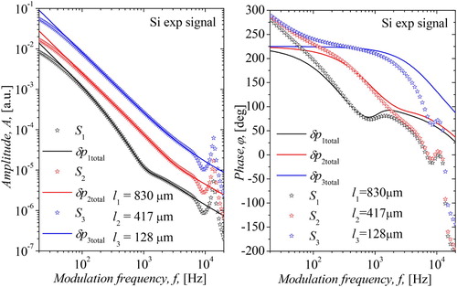
In order to validate our ANN choice, independent PA measurements were used with the same frequency step and the range of the parameter values as those used for the network training. The open photoacoustic cell OPC [12,13,28] experimental set-up was used, explained in detail elsewhere [12,13,28]. As a detector, standard electret microphone ECM30B was used together with a laser diode of 660 nm wavelength and 20 mW of power as a light source modulated with a current modulator in the frequency range of 20 Hz–20 kHz. All our measurements were performed using circular plates made of n-type silicon as a well-known material having the radius of $R_s=4\text{ mm}$ and different thicknesses l: 830, 417 and 128 µm. Experimental signal $S(f)$ (a) amplitudes A and (b) phases ϕ were obtained from these samples, (Figure 5, asterisks). Following signal correction procedure explained earlier, the rectified (‘true’) PA signal $\delta p_{\text{total}}(f)$ (a) amplitudes $A_{\text{total}}(f)$ and (b) phases ${\phi }_{\text{total}}(f)$ are obtained (Figure 5, solid lines), applying H(f) results from previous analysis [12,13]. Rectified signals presented in Figure 5 fairly represent the signals from the silicon sample having these parameters: thermal diffusivity D_T = 9.0×10⁻⁵m²s⁻¹ and thermal expansion α_T = 2.6×10⁻⁶ κ⁻¹. In our further analysis, these parameters will be compared to the ANNs prediction.

Figure 5. Frequency dependence: (a) amplitudes and (b) phases in experimental measurements of photoacoustic signals$S(f)$ (stars) of three n – type silicon samples (thickness l₁=830 µm, l₂=417 µm and l₃=128 µm) and the corresponding fit of experimental photoacoustic (a) amplitudes and (b) phases (line) after removing instrumental deviations.

The ‘true’ $A_{\text{total}}(f)$ and ${\phi }_{\text{total}}(f)$ from Figure 5 are scaled using amplitude normalization procedure, so $A_n=20\log A_{\text{total}}(f)$ together with ${\phi }_{\text{total}}(f)$, as the function of modulated frequencies f (Figure 6), were presented to our neural networks. The prediction results $D_{\text{T}}^{\text{ANN}}$, ${\alpha }_{\text{T}}^{\text{ANN}}$ and $l^{\text{ANN}}$ of ANN1, ANN2 and ANN3 are given in Table 2. Errors are obtained comparing network predictions with$D_{\text{T}}$, ${\alpha }_{\text{T}}$ and $l$ obtained after PA signal rectification. It is obvious that the best predictions (minimum errors) are achieved using the ANN1 network trained with amplitude and phase data simultaneously as inputs. This result confirms our assumption that PA signal analysis is correct and reliable only when amplitudes and phases are included simultaneously. Working only with amplitudes or phases could lead to significant mistakes: not only larger errors but the combination of obtained parameters values could be far from the reality.

Figure 6. PA signal $\delta p_{\text{total}}(f)$ (a) normalized values of $A_{\text{total}}(f)$ and (b) values of ${\phi }_{\text{total}}(f)$ obtained for three different thicknesses l presented to the neural networks for the prediction test.

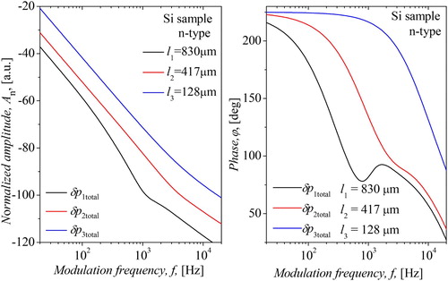
Table 2. Values of $D_{\text{T}}^{\text{ANN}}$, ${\alpha }_{\text{T}}^{\text{ANN}}$ and $l^{\text{ANN}}$ predicted by different neural networks for three samples.

	Sample no. 1			Sample no.2			Sample no. 3
	$D_{\text{T}}^{\text{ANN}}$	${\alpha }_{\text{T}}^{\text{ANN}}$	$l^{\text{ANN}}$	$D_{\text{T}}^{\text{ANN}}$	${\alpha }_{\text{T}}^{\text{ANN}}$	$l^{\text{ANN}}$	$D_{\text{T}}^{\text{ANN}}$	${\alpha }_{\text{T}}^{\text{ANN}}$	$l^{\text{ANN}}$
ANN parameters unit	$[\text{1}{\text{0}}^{-\text{5}}{\text{m}}^{\text{2}}{\text{s}}^{-1}]$	$[\text{1}{\text{0}}^{-\text{6}}{\text{K}}^{-\text{1}}]$	$[{10}^2\mu \text{m}]$	$[\text{1}{\text{0}}^{-\text{5}}{\text{m}}^{\text{2}}{\text{s}}^{-1}]$	$[\text{1}{\text{0}}^{-\text{6}}{\text{K}}^{-\text{1}}]$	$[{10}^2\mu \text{m}]$	$[\text{1}{\text{0}}^{-\text{5}}{\text{m}}^{\text{2}}{\text{s}}^{-1}]$	$[\text{1}{\text{0}}^{-\text{6}}{\text{K}}^{-\text{1}}]$	$[{10}^2\mu \text{m}]$
ANN1	9.0030	2.5995	8.2998	8.9994	2.5993	4.1687	9.0093	2.5952	1.2802
Error	0.0030	0.0005	0.0002	0.0006	0.0007	0.0013	0.0093	0.0048	0.0002
ANN2	9.0048	2.5591	8.2991	9.0123	2.6016	4.1728	9.8222	2.5042	1.4132
Error	0.0048	0.0009	0.0009	0.0123	0.0016	0.0028	0.8222	0.0958	0.1332
ANN3	9.0014	2.5994	8.2990	8.9965	2.6040	4.1691	11.6601	2.2463	1.4599
Error	0.0014	0.0006	0.0010	0.0035	0.0040	0.0009	2.6601	0.3537	0.1799

Note: Errors, which represent the difference between the ANN predicted and standard PA calculated D_T, α_T and l values are also shown.

Also, sample thickness plays a very important role in the consideration of network precision efficiency. The results presented in Table 2 support that remark. For example, the ANN3 prediction of all parameters, especially $D_{\text{T}}$, is very precise in the case of thicker samples (l >> L) [24], losing that precision significantly in the case of thinner ones ($l\to L$) [23]. The same could be observed in the case of ANN2.

Now, to solve our inverse problem and to perform full characterization of the sample [29–32] in frequency domain, the ANN1 prediction of $D_{\text{T}}^{\text{ANN}}$, ${\alpha }_{\text{T}}^{\text{ANN}}$ and $l^{\text{ANN}}$ has to be returned to the model equations (2–5) to obtain and all of its components: $\delta p_{\text{TD}}(f)$, $\delta p_{\text{TE}}(f)$, and $\delta p_{\text{PE}}(f)$. In such a way the influence and domination of TD, TE and PE effects in different frequency ranges can be found [12,16–18]. In other words, complete thermal and electronic characterization of the sample can be achieved, knowing that $D_{\text{T}}^{\text{ANN}}$ and ${\alpha }_{\text{T}}^{\text{ANN}}$ are temperature dependent parameters: $D_{\text{T}}^{\text{ANN}}$ is closely connected to the TD effects and ${\alpha }_{\text{T}}^{\text{ANN}}$ is closely connected to the TE effects. Both TD and TE effects are dependent on heat conduction process in the sample (temperature gradient existence) and $l^{\text{ANN}}$. In the case of PE effect, it is purely electronic (non thermal) effect which explains sample bending due to mechanical stress caused by excess carrier generation. It means that PE effect is strongly related to $l^{\text{ANN}}$ and minority carrier concentration $\delta n_p(x,f)$. In the case of plasma-thick samples PE effect is negligible, so our focus will be on the sample thermal characterization. The results of this analysis are shown in Figures 7–9.

Figure 7. Frequency characterization of the total photoacoustic signal of the n-type silicon sample with the thermodiffusion, thermoelastic and plasmaelastic components, for the parameters $D_{\text{T}}^{\text{ANN}}$= 9.0030×10⁻⁵ m²s⁻¹ and ${\alpha }_{\text{T}}^{\text{ANN}}$= 2.5995×10⁻⁶ κ⁻¹ obtained by the neural network for sample thickness of $l_{\text{1}}^{\text{ANN}}$= 829.98 µm.

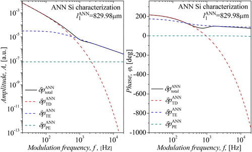
Figure 8. Frequency dependence of the total photoacoustic signal and its three components for a silicon sample for parameter values of the neural network prediction $l_2^{\text{ANN}}$= 416.87 µm, $D_{\text{T}}^{\text{ANN}}$= 8.9994×10⁻⁵ m²s⁻¹ and ${\alpha }_{\text{T}}^{\text{ANN}}$= 2.5993×10⁻⁶ κ⁻¹.

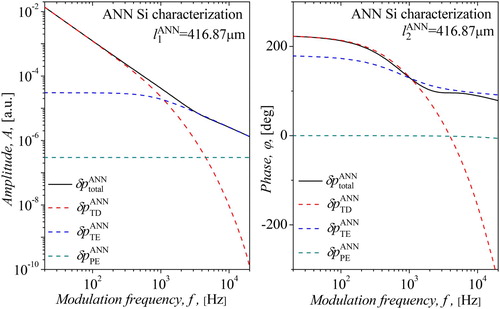
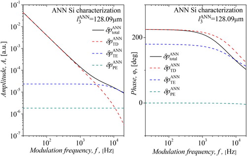
Figure 9. Characterization of a silicon sample in the frequency domain, after parameter prediction by neural networks $l_3^{\text{ANN}}$= 128.02 µm, $D_{\text{T}}^{\text{ANN}}$= 9.0093×10⁻⁵ m²s⁻¹ and ${\alpha }_{\text{T}}^{\text{ANN}}$= 2.5952×10⁻⁶ κ⁻¹. The characterization is given by photoacoustic signals with thermodiffusion, thermoelastic and plasmaelastic components.

It is clear from these pictures that the TD effect (the thermal piston effect) dominates in the low-frequency range (Figure 7 – $\delta p_{\text{TD}}^{\text{ANN}}(f)$ dominates in $\delta p_{\text{total}}^{\text{ANN}}(f)$ at f < 10³ Hz). The $\delta p_{\text{TD}}^{\text{ANN}}(f)$ brings the information about the heat conduction within the sample, allowing one to extract sample density, specific heat and thermal conductivity as parameters closely related to the sample material. By reducing the sample thickness, the domination of the $\delta p_{\text{TD}}^{\text{ANN}}(f)$ component becomes obvious in much wider frequency domain (Figures 8 and 9). It means that in PA measurements thinner samples are much more convenient to investigate, in terms of the calculation of heat conduction parameters. At higher frequencies, TE effects (effects of a mechanical piston) dominate (Figure 9 – $\delta p_{\text{TE}}^{\text{ANN}}(f)$ component dominates in $\delta p_{\text{total}}^{\text{ANN}}(f)$ at f > 10⁴ Hz). It means that $\delta p_{\text{TE}}^{\text{ANN}}(f)$ brings the information about the temperature gradient in the sample, allowing one to extract temperatures at sample surfaces and some elastic parameters of the sample material (Young`s modulus for example). By increasing the thickness, the domination of the $\delta p_{\text{TE}}^{\text{ANN}}(f)$ component becomes apparent in much wider frequency range (Figures 7 and 8). It means that in PA measurements thicker samples are much more convenient to investigate, in terms of the calculation of elastic parameters. In all (Figures 7–9) the influence of the PE effect, i.e. the influence of $\delta p_{\text{PE}}^{\text{ANN}}(f)$ component on $\delta p_{\text{total}}^{\text{ANN}}(f)$, is negligible. The obtained results depicted in the mentioned figures correspond to the typical behaviour of plasma-thick semiconductor samples.

4. Conclusion

The main idea presented in this article is to solve the inverse problem in semiconductor photoacoustics which consists of using the results of actual photoacoustic measurements of n-type silicon plates (signal amplitudes and phases) to infer about the sources of the signal behaviour (thermal diffusion, thermoelastic and plasmaelastic effects) in the 20 Hz–20 kHz frequency domain. Undistorted measured photoacoustic signals are presented to the different artificial neural networks trained with different inputs (only amplitudes, only phases, both) of the large set of the theoretical data to obtain sample parameters (thermal diffusivity, thermal expansion, and thickness). The results of training indicate that all networks give accurate values of the investigated samples but the network trained with both PA amplitudes and phases simultaneously outperform the other two approaches reaching the required precision and accuracy of the parameter prediction in real – time. Sample parameters obtained with such networks are returned to the theoretical model to calculate the photoacoustic signal components resulting from the aforementioned effects. Identifying the frequency domains in which the individual components dominate allows one to perform a complete characterization of the semiconductor using the correlation between the identified sources (effects) of the signal behaviour and associated physical processes that characterize the investigated material. This kind of analysis demonstrates the potential and utility of the presented idea to solve the problems from a diverse set of application areas (material characterization, environmental sciences, electronics, sensor networks, etc.).

Disclosure statement

No potential conflict of interest was reported by the author(s).

Additional information

Funding

This work was supported by the Ministry of Education, Science and Technological Development of the Republic of Serbia under projects No. ON171016 and III45005.

Appendix

The samples are n-type silicon circular plates of the radius R_s=4 mm and thicknesses 830, 417 and 128 µm. The characteristic bulk lifetime of minority carriers is τ=5µs, as specified in early measurements [23].

Table A1. Values of silicon parameters used for fitting

Parameters	Labels	Values
Thermal diffusivity of air	Dg[m^2s^−1]	2.0566×10^−5
Standard temperature	T0[K]	300
Standard pressure	p0[Pa]	10^5
Adiabatic index for air	$\gamma$	1.4
Diffusion length of minority carrier	Lp[m]	77.46×10^−6
Coefficient of minority carrier diffusivity	Dp[m^2s^−1]	1.2×10^−3
Recombination velocity of the front surface	s1[ms^−1]	2
Recombination velocity of the rear surface	s2 [ms^−1]	24
Photon energy	ε0[J]	3.01×10^−19
Energy gap for silicon	εg [J]	1.78×10^−19
Thermal conductivity	k[Wm^−1K^−1]	150.0
Optical absorption	β[m^−1]	2.58×10^5
Coefficient of electronic deformation	dn[m^3]	−9×10^−31
Optical reflectivity	Reflek[m^−1]	0.35

References

- Mandelis A, editor. Photoacoustic and thermal wave phenomena in semiconductors. New York (NY): Elsevier, 1987. ISBN-10: 0444012265
- Mandelis A, Hess P, editors. Semiconductors and electronic materials. Vol. IV in the Series: Progress in photothermal and photoacoustic science and technology. Bellingham: SPIE Press, 2000. p. 271–315. ISBN: 9780819435064
- Rosencwaig A, Gersho A. Theory of the photoacoustic effect with solids. J Appl Phys. 1976;47:64. doi: 10.1063/1.322296
- McDonald F, Wetsel G. Generalized theory of the photoacoustic effect. J Appl Phys. 1978;49:2313. doi: 10.1063/1.325116
- Da Silva MD, Bandeira IN, Miranda LCM. Open-cell photoacoustic radiation detector. J Phys E, Sci Instrum. 1987;20:12. doi: 10.1088/0022-3735/20/12/009
- Perondi LF, Miranda LCM. Minimal-volume photoacoustic cell measurement of thermal diffusivity: effect of the thermoelastic sample bending. J Appl Phys. 1987;62:2955. doi: 10.1063/1.339380
- Balderas-Lopez JA, Mandelis A. Thermal diffusivity measurements in the photoacoustic open-cell configuration using simple signal normalization techniques. J Appl Phys. 2001;90:2273. doi: 10.1063/1.1391224
- Todorovic DM, Nikolic PM, Bojicic AI, et al. Thermoelastic and electronic strain contribution to the frequency transmission photoacoustic effect in semiconductors. Phys Rev B. 1997;55:15631–15642. doi: 10.1103/PhysRevB.55.15631
- Duch W, Diercksen GHF. Neural networks as tools to solve problems in physics and chemistry. Comput Phys Commun. 1994;82(2–3):91–103. doi: 10.1016/0010-4655(94)90158-9
- Artrith N, Urban A. An implementation of artificial neural-network potentials for atomistic materials simulations: performance for TiO2. Comput Mater Sci. 2016;114:135–150. doi: 10.1016/j.commatsci.2015.11.047
- Ćojbašić Z, Nikolić V, Ćirić I, et al. Computationally intelligent modelling and control of fluidized bed combustion process. Therm Sci. 2011;15:321. doi: 10.2298/TSCI101205031C
- Markushev DD, Rabasovic MD, Todorovic DM, et al. Photoacoustic signal and noise analysis for Si thin plate: signal correction in frequency domain. Rev Sci Instrum. 2015;86:035110. doi: 10.1063/1.4914894
- Aleksić SM, Markushev DK, Pantić DS, et al. Electro-acoustic influence of the measuring system on the photoacoustic signal amplitude and phase in frequency domain. Facta Universitatis Ser: Phys Chem Technol. 2016;14(1):9–20. doi: 10.2298/FUPCT1601009A
- Lukić M, Ćojbašić Ž, Rabasović MD, et al. Computationally intelligent pulsed photoacoustics. Meas Sci Technol. 2014;25:12. doi:10.1088/0957- 0233/25/12/125203 doi: 10.1088/0957-0233/25/12/125203
- Lukić M, Ćojbašić Ž, Rabasović MD, et al. Neural networks-based real-time determination of laser beam spatial profile and vibrational-to translational relaxation time within pulsed photoacoustics. Int J Thermophys. 2013;34(8–9):1795–1802. doi: 10.1007/s10765-013-1507-y
- Djordjevic KL, Markushev DD, Ćojbašić ŽM, et al. Photoacoustic measurements of the thermal and elastic properties of n-type silicon using neural networks. Silicon. 2019 doi: 10.1007/s12633-019-00213-6
- Todorović DM, Nikolić PM, Dramićanin MD, et al. Photoacoustic frequency heat-transmission technique: thermal and carrier transport parameters measurements in silicon. J Appl Phys. 1995;78(9):5750. mailto:[email protected] doi: 10.1063/1.359637
- Todorović DM, Nikolić PM. Semiconductors and electronic materials progress in photothermal and photoacoustic, science and technology Chap. 9. New York (NY): Optical Engineering Press 2000. p. 273–318.
- Dramićanin MD, Nikolić PM, Ristovski ZD, et al. Photoacoustic investigation of transport in semiconductors: theoretical and experimental study of a Ge single crystal. Phys Rev B. 1995;51:4226. doi: 10.1103/PhysRevB.51.14226
- Gurevich YG, Lashkevych II. Sources of Fluxes of energy, heat, and diffusion heat in a bipolar semiconductor: influence of nonequilibrium charge carriers. Int J Thermophys. 2013;34:341. doi: 10.1007/s10765-013-1416-0
- De la Cruz GG, Gurevich YG. Electron and phonon thermal waves in semiconductors: an application to photothermal effects. J Appl Phys. 1996;80:1726. mailto:[email protected] doi: 10.1063/1.362971
- Marin E, Vargas H, Diaz P, et al. On the photoacoustic characterization of semiconductors: influence of carrier recombination on the thermodiffusion, thermoelastic and electronic strain signal generation mechanisms. Phys Status Solidi A-Appl. 2000;179:387. doi:10.1002/1521-396X(200006)179:23.0.CO;2-Y doi: 10.1002/1521-396X(200006)179:2<387::AID-PSSA387>3.0.CO;2-Y
- Markushev DK, Markushev DD, Galović S, et al. The surface recombination velocity and bulk lifetime influences on photogenerated excess carrier density and temperature distributions in n-type silicon excited by a frequency-modulated light source. Facta Universitatis Ser: Electron Energ. 2018;31(2):313–328. doi: 10.2298/FUEE1802313M
- Markushev DK, Markushev DD, Aleksic SM, et al. Effects of the photogenerated excess carriers on the thermal and elastic properties of n-type silicon excited with a modulated light source: theoretical analysis. J Appl Phys. 2019;126:185102. doi: 10.1063/1.5100837
- Popović MN, Nešić MV, Cirić-Kostić S, et al. Helmholtz resonances in photoacoustic experiment with laser-sintered polyamide including thermal memory of samples. Int J Thermophys. 2016;37:116. doi: 10.1007/s10765-016-2124-3
- Sola J, Sevilla J. Importance of input data normalization for the application of neural networks to complex industrial problems. IEEE Trans Nucl Sci. 1997;44(3):1464–1468. doi: 10.1109/23.589532
- Wang LY, Yin GG, Zhao Y, et al. Identification input design for consistent parameter estimation of linear systems with binary-valued output observations. IEEE Trans Automat Contr. 2008;53(4):867–880. doi: 10.1109/TAC.2008.920222
- Marquard DW. An algorithm for least-squares estimation of nonlinear parameters. J Soc Ind Appl Math. 11(2):431–441. doi: 10.1137/0111030
- Rabasović MD, Nikolić MG, Dramićanin MD, et al. Low-cost, portable photoacoustic setup for solid state. Meas Sci Technol. 2009;20:9. doi: 10.1088/0957-0233/20/9/095902
- Glorieux C, Thoen J. Thermal depth profile reconstruction by neural network recognition of the photothermal frequency spectrum. J App Phys. 1996;80(11):6510–6514. doi: 10.1063/1.363670
- Glorieux C, Li Voti R, Thoen J, et al. Depth profiling of thermally inhomogenous materials by neural network recognition of photothermal time domain data. J App Phys. 1999;85(10):7059–7063. doi: 10.1063/1.370512
- Popovic MN, Furundzic D, Galovic SP. Photothermal depth profiling of optical gradient materials by neural network. Publ Astron Obs Belgrade. 2010;89:2015.