Seismic inversion constrained by stress value changes

ABSTRACT

Seismic inversion is an effective way to get stress distribution of rock in coal mine, but its usage is still limited by multi-solution problem in practice. As seismometers can only be deployed in limited areas in underground coal mine, it is impossible to solve multi-solution problem by adding more seismometers, thus, we propose a new seismic inversion method which introduces stress value changes as constraint to solve this problem. Numerical experiments show that the new method can reduce the mean distance between inversion results and true wave velocity distributions by about 11.5%, reduce the variance of the distances by about 91%, reduce the mean distance between inversion results and frequency-domain-truncated true wave velocity distributions by about 30.6% and reduce the variance of the distances by about 84.1%. These results indicate that the new method proposed in this paper can reduce the non-uniqueness of solutions in seismic inversion and improve the reliability and stability of seismic inversion.

KEYWORDS:

• Seismic inversion
• stress value
• dimension reduction
• FFT
• PSO

2010 Mathematics Subject Classification:

• 86-08

1. Introduction

Coal-gas outburst is a major risk in underground coal mine and often leads to a great loss of life and property. As presently there is no technique to monitor directly the stress exerted on surrounding rocks, monitoring the seismic wave velocity distribution becomes the most popular technique used in coal mine disaster prediction [1]. But in the practice, the result is usually not unique [2] due to incompleteness of measured data, measurement error or model error, etc. There are two main criteria to solve the multi-solution problem in seismic inversion: better model parameterization method and introducing more constraints in the inversion.

Regular parameterizations are simple and easy to use but cannot adjust the mesh according to uneven data coverage. Irregular parameterizations, especially transform domain methods are more effective due to the utilization of natural sparsity of model parameters in transform domain. Transform domain methods have been used in global body wave imaging widely and have got excellent results: Tikhotsky et al. [3] reduced dimension number of model space to 3% by two-dimensional Haar wavelet and got results very close to true value, which indicates the feasibility of this idea. Jean et al. [4] used the sparsity of model in transform domain to constrain inversion process and got results consistent with predecessors without making any geometric assumption on the mesh, and this indicates that the sparsity of model in transform domain is ubiquitous.

It is impossible to completely solve multi-solution problem in seismic inversion by only introducing better parameterization methods. Syracuse et al. [5] used a combination of body wave time, surface wave frequency dispersion and gravity data to invert P and S wave velocities simultaneously. The higher resolution they achieved indicate how the introduction of multiple types of parameters can improve the inversion resolution. Demirci et al. [6] proposed a new method based on cross-gradient to invert deep structure from magnetotelluric data and seismic data, concluding that the joint inversion can increase the resolution of deep structures and is stable.

The target area of seismic inversion in underground coal mine is relatively small and some parts of it are accessible to people, thus helping the deployment of various types of sensors, as stress meters. However, it is difficult to get a continuous and exact stress value in underground coal mine. The frequently used stress relief method [7] can get the exact stress value but is not convenient to use and cannot monitor continuously. Borehole stress meter [8] is another frequently used equipment and can work continuously but cannot provide the exact stress value. As the ultimate goal of seismic inversion in underground coal mine is monitoring the stress distribution of target area continuously, it is more appropriate to introduce stress value changes rather than exact stress value to improve seismic inversion result. According to the study of Gong [9], axial stress exerted on coal rock sample and longitudinal wave velocity of it are in accordance with power function relationship in elastic deformation stage, thus we can use this relation to create some constraints to improve seismic inversion result. Moreover, to reduce the difficulty of inversion, sparse representation of model can still be introduced to seismic inversion to reduce number of model parameters. Based on this idea, we propose a new seismic inversion method constrained by stress value changes, and numerical experiments show that the new method can effectively improve the stability and reliability of seismic inversion.

2. Methodology

2.1. Minimize model space size

A model $m$ described by $n$ model parameters in seismic inversion, is a particular choice of model parameters set used to describe target area, a model space is a collection of models which are generated based on same rules. If there are no limitations on values of model parameters, the model can be treated as a point in ${\mathit{R}}^n$. The model can also be treated as a point in ${\mathit{L}}^2({\mathit{R}}^2)$ space (for two-dimensional target area) or a point in ${\mathit{L}}^2({\mathit{R}}^3)$ space (for three-dimensional target area) if we define the coordinates of a point in target area as inputs and define the velocity or other geological parameters of the point as output of a function. But, in practice, the target area is always parameterized by constant-velocity cells (for two-dimensional target area) or constant-velocity blocks (for three-dimensional target area), that is the inputs of the model are discrete, thus the model should be treated as a point in ${\mathit{l}}^2({\mathit{R}}^2)$ or ${\mathit{l}}^2({\mathit{R}}^3)$.

A model in ${\mathit{L}}^2({\mathit{R}}^2)$ or ${\mathit{L}}^2({\mathit{R}}^3)$ can be wrote as $m={\sum }_{q=1}^r{a}_q{\psi }_q$, where $\mathit{\psi }=({\psi }_1,{\psi }_2,\dots ,{\psi }_q,\dots ,{\psi }_r)$ is an orthonormal basis of ${\mathit{L}}^2$ space (e.g. wavelet, Fourier) and $\mathit{a}=(a_1,a_2,\dots ,a_q,\dots a_r)$ is the coefficient vector [10]. If there are $r-k$ coefficients in $\mathit{a}$ equal to 0 or near 0, and there is $k\ll r$, the model $m$ is called k-sparse in orthonormal basis $\mathit{\psi }$. Similarly, we can get the sparse representations of a discrete model in ${\mathit{l}}^2({\mathit{R}}^2)$ or ${\mathit{l}}^2({\mathit{R}}^3)$ based on discrete orthogonal transformations [11], and in general, there is $k\ll n$. If all the models in an n-dimensional model space ${\mathit{R}}^n$ have k-sparse representations and the $k$ coefficients are all real, then we can get a dimension reduced model space ${\mathit{R}}^k$ which contains all the models.

Reduction of dimensions leads to reduction of the model space size, but before we get into the discussion about this, the definition of the model space size should be discussed first. If the values in each dimension of the model space are continuous, we cannot compare the size of two model spaces that have different dimension numbers. But if the values in each dimension are discrete, the model space will consist of a finite number of models, and the number of models is equal to the product obtained by multiplying the number of the possible values in each dimension. Since a seismic inversion program always runs on computer and the precision of data in computer is always finite, the number of the values in each dimension of a model space must be finite when the precision of each dimension is determined; therefore, the size of model space must be calculable in practice. Define $S{M}^n$ as the size of an n-dimensional model space, there is $S{M}^n\text{ = }n{v}_1\times n{v}_2\times \cdots \times n{v}_p\times \cdots \times n{v}_n$, where $n{v}_p$ is the number of values in the $p_{th}$ dimension of model space, and naturally there is $n{v}_p\ge 1$. Assuming the $(p-1{)}_{th}$ dimension and the $p_{th}$ dimension are merged into a new dimension and numbers of values in other dimensions remain unchanged, the number of values in the merged new dimension will be $n{v}_{p-1}+n{v}_p$, size of the new $n-1$ dimension model space will be: $S{M}^{n-1}=n{v}_1\times n{v}_2\times \cdots \times (n{v}_{p-1}+n{v}_p)\times \cdots \times n{v}_n=S{M}^n\times \left(\frac{1}{n{v}_{p-1}}+\frac{1}{n{v}_p}\right)$As the number of values in a dimension is usually much larger than 1, so we can get $S{M}^{n-1}\le S{M}^n$ in most cases. This result indicates that we can reduce the model space size by reducing the dimensions of model space.

According to the idea discussed above, here we use Fourier transform to get sparse representation of a model and try to find the optimal model in frequency domain.

Two-dimensional DFT formula of an A*B image is (1) $F({\xi }_1,{\xi }_2)=\mathcal{F}(f(x_1,x_2))=\sum _{x_1=0}^{A-1}\sum _{x_2=0}^{B-1}f(x_1,x_2)e^{-2\pi i((x_1{\xi }_1/A)+(x_2{\xi }_2/B))}$(1) and the inverse transform is (2) $f(x_1,x_2)={\mathcal{F}}^{-1}(F({\xi }_1,{\xi }_2))=\frac{1}{AB}\sum _{{\xi }_1=0}^{A-1}\sum _{{\xi }_2=0}^{B-1}F({\xi }_1,{\xi }_2)e^{2\pi i((x_1{\xi }_1/A)+(x_2{\xi }_2/B))}$(2) The $F({\xi }_1,{\xi }_2)$ in Formula (1) satisfies Equations (3)–(5) and the number of values in discrete variables ${\xi }_1$ and ${\xi }_2$ are equal to A and B. (3) $\begin{array}{rl}|F(\mathit{\xi })|& =|F(-\mathit{\xi })|\end{array}$(3) (4) $\begin{array}{rl}{\phi }_{F(\mathit{\xi })}& =-{\phi }_{F(-\mathit{\xi })}\text{when}\mathit{\xi }\ne 0\end{array}$(4) (5) $\begin{array}{rl}{\phi }_{F(\mathit{\xi })}& =0\text{when}\mathit{\xi }=0\end{array}$(5) where $\mathit{\xi }=({\xi }_1,{\xi }_2)$.

Figure 1(a) shows a 50*50 sample image, its magnitude spectra and coordinate system in frequency domain are shown in Figure 1(b).

Figure 1. Sample image and its coordinate system in frequency domain. (a) 50*50 sample image. (b) Coordinate system of the sample image in frequency domain.

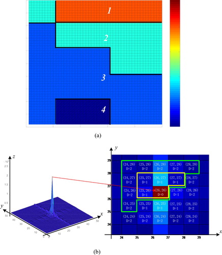
The variable $D$ in Figure 1(b) is the distance from one cell to the center cell (26, 26). The number of complex values need to handle in frequency domain will be $2D^2+2D+1$ according to the symmetry shown in Equations (3) and (4). For example, as shown in Figure 1(b), the variables surrounded by the smaller box are the variables need to handle when $D=1$ and the larger box encircles the variables need to handle when $D=2$. To discuss seismic inversion in ${\mathit{R}}^n$, we should use real numbers to represent a model, thus number of real values need to handle is (6) $2\times (2D^2+2D+1)-1=4D^2+4D+1$(6) The subtracted number ‘1’ in Equation (6) represents the argument of the complex value locates in (26, 26) in Figure 1(b) and the reason why we subtract it is shown in Equation (5). Thus we can carry out an optimization process in ${\mathit{R}}^{4D^2+4D+1}$ rather than ${\mathit{R}}^{2500}$.

2.2. Introduce stress value changes as constraint

In this paper, we use particle swarm optimization (PSO) to carry out seismic inversion in the dimension reduced model space. PSO, which is first introduced by Kennedy and Eberhart [12], is a stochastic global optimization technique inspired by social behaviour of bird flocking or fish schooling. In PSO algorithm, a number of agents called particles are placed in model space to find optimal position which can minimize fitness function (or objective function). Figure 2 demonstrates the workflow of PSO algorithm.

Figure 2. Workflow of PSO algorithm.

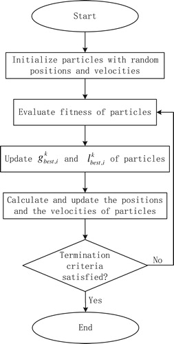
The $l_{best,i}^k$ in Figure 2 is the best position where the $i_{th}$ particle has arrived until iteration $k$, $g_{best,i}^k$ is the best position where all particles have arrived until iteration $k$. From Figure 2 we can see that, fitness function and termination criteria are key factors in PSO Algorithm.

As we want to introduce stress value changes as constraint, we have to invert the wave velocity distribution before and after stress change simultaneously. Named the observation collection vector before stress change as $d^{obs,b}$, the observation collection vector after stress change as $d^{obs,a}$, we define the first arrival times as observations. The fitness function $f^{obj}$ is (7) $f^{obj}((m^b,m^a))=S\times ({\Vert d^{obs,b}-G({\mathcal{F}}^{-1}(m^b))\Vert }_2+{\Vert d^{obs,a}-G({\mathcal{F}}^{-1}(m^a))\Vert }_2)$(7) Vector $m^b$ and $m^a$ are models in model space ${\mathit{R}}^{4D^2+4D+1}$ which represent the target area before and after the stress change respectively, being both sparse representations of spatial model.

Named space-domain representation of model before stress change as ${\mathcal{F}}^{-1}(m^b)$ and the model after stress change as ${\mathcal{F}}^{-1}(m^a)$, the velocities in ${\mathcal{F}}^{-1}(m^b)$ and ${\mathcal{F}}^{-1}(m^a)$ should be rounded to integers range from 0 to 255 as mentioned in Section 2.1. It is important to note that the geologic parameter of each cell in ${\mathcal{F}}^{-1}(m^b)$ or ${\mathcal{F}}^{-1}(m^a)$ should be the longitudinal wave velocity of target area, and the velocity distributes uniformly in each cell.

Function $G$ in Equation (7) relates model and observations, and here we use ray tracing [13] to establish this relation.

The parameter $S$ in Equation (7) is the penalty factor about stress value change. $S$ should be set to 1 when all the velocities of cells in ${\mathcal{F}}^{-1}(m^b)$ and ${\mathcal{F}}^{-1}(m^a)$ have the same directions of change (that is greater, less or equal) with the stress values of the same cells in which the stress meters are placed in; otherwise, $S$ should be set to 2.

The termination criteria is set to iterative 30 times in this paper and of course, we may use also other termination criteria, such as gradient of optimal solution, variance of all the solutions, etc.

Furthermore, to accelerate the convergence, all the initial particles which do not match the known directions should be eliminated and regenerated.

3. Experiments and analysis

3.1. Feasibility experiment and analysis

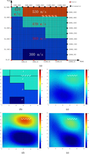
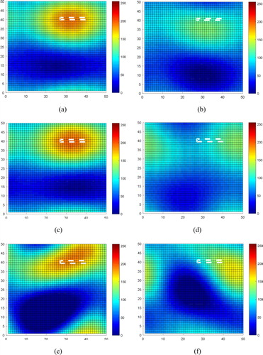
The feasibility experiment is designed based on Figure 1(a) to reuse analysis results in previous sections. Figure 3(a) shows the actual wave velocity distribution, the actual coordinates of sources and seismometers before stress change. The cells in the white dotted box shown in Figure 3 indicate positions where stress meters are placed in; the actual wave velocities in Figure 3(a) range from 300 to 600 m/s and are mapped to integers range from 0 to 255 as shown in Figure 1(a). Assuming that the stress exerted on area 1 decreased, the velocities of cells in this area should decrease simultaneously; Figure 3(b) shows the normalized wave velocity distribution after stress change. Named the theoretical first arrival times before and after stress change as $d^{obs,b}$ and $d^{obs,a}$ and treat them as observations, we set $D=1$.

Figure 3. Feasibility experiment results. (a) Actual wave velocities and coordinates. (b) Normalized true wave velocity distribution after stress change. (c) Normalized true wave velocity distribution after stress change when $D\text{ = 1}$. (d) Inversion result before stress change when $D\text{ = 1}$. (e) Inversion result after stress change when $D\text{ = 1}$.

Organization of $m^{ba}$ is $\begin{array}{rl}& (mod{\text{1}}_{(25,27)},ang{\text{1}}_{(25,27)},mod{\text{1}}_{(26,27)},ang{\text{1}}_{(26,27)},mod{\text{1}}_{(25,26)},ang{\text{1}}_{(25,26)},\\ & mod{\text{1}}_{(26,26)},ang{\text{1}}_{(26,26)},mod{\text{1}}_{(25,25)},ang{\text{1}}_{(25,25)},mod{2}_{(25,27)},ang{2}_{(25,27)},\\ & mod{2}_{(26,27)},ang{2}_{(26,27)},mod{2}_{(25,26)},ang{2}_{(25,26)},mod{2}_{(26,26)},ang{2}_{(26,26)},\\ & mod{2}_{(25,25)},ang{2}_{(25,25)})\end{array}$where $mod{\text{1}}_{(25,27)}$ and $ang{\text{1}}_{(25,27)}$ are the module and argument of Fourier coefficient located in (25,27) as shown in Figure 1(b) and other elements are similarly. The last number 1 in $mod{\text{1}}_{(25,27)}$ and $ang{\text{1}}_{(25,27)}$ indicates that the values belong to the model before stress change; otherwise, the number should be 2.

Upper and lower limits of $m^{ba}$ are $\begin{array}{rl}& ({10}^5,180,{10}^5,180,{10}^5,180,3\times {10}^5,0,{10}^5,180,{10}^5,180,{10}^5,180,{10}^5,180,3\\ & \times {10}^5,0,{10}^5,180,{10}^5,180,{10}^5,180,{10}^5,180,3\times {10}^5,0,{10}^5,180,{10}^5,180,{10}^5,180,{10}^5,\\ & 180,3\times {10}^5,0,{10}^5,180)\end{array}$and $\begin{array}{rl}& (0,-180,0,-180,0,-180,1.5\times {10}^5,0,0,-180,0,-180,0,-180,0,-180,1.5\times {10}^5,0,\\ & 0,-180,0,-180,0,-180,0,-180,1.5\times {10}^5,0,0,-180,0,-180,0,-180,0,-180,1.5\\ & \times {10}^5,0,0,-180)\end{array}$We set the number of particles equal to 32 to match the core number of server, and set the maximum number of iterations to 30. The inversion results are shown in Figure 3(d) and (e), and other indicators which change with iterations are shown in Figure 4. The ‘Global Best’ in Figure 4(a) is the fitness function value of the global best particle in each iteration, and the ‘Mean’ is the mean fitness function values of all particles in each iteration.

Figure 4. Energy ratio and distance of feasibility experiment results. (a) Global best and mean fitness function values. (b) Energy ratio of inversion results to true velocity distributions. (c) Distance between inversion results and true velocity distributions.

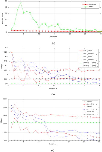
The meanings of the symbols used in Figure 4 are shown in Table 1.

Table 1. Meanings of symbols in feasibility experiment.

Symbol	Meaning
rb	Inversion result before stress change
ra	Inversion result after stress change
mb	True model before stress change as shown in Figure 1(a)
ma	True model after stress change as shown in Figure 3(b)
mbD1	Frequency-domain-truncated true model before stress change when $D\text{ = 1}$
maD1	Frequency-domain-truncated true model after stress change when $D\text{ = 1}$ as shown in Figure 3(c)

Following conclusions can be drawn from Figures 3 and 4:

1. Seismic inversion constrained by stress value change is convergent. As can be seen from Figure 4, the ‘Global Best’ curve decreases as the number of iterations increases, and this is consistent with the convergence characteristics of PSO. The ‘Mean’ curve reflects the dispersion of particles in inversion process, as shown in Figure 4, it decreases in general but fluctuates locally. The reason of the local fluctuations arise is the parameter $S$ in Equation (7), which doubles the fitness function value if wave velocity distributions do not match the measured direction of stress value.

2. Figure 4(b,c) demonstrates the tendency of final inversion results, the targets are more like the ideal low pass filtered true models rather than the true models and this tendency is more noticeable in Figure 4(c). Thus the ‘Distance’, as shown in Figure 4(c) is more a clarity indicator to demonstrate the closeness of inversion results to true models rather than the energy ratio, as shown in Figure 4(b).

3.2. Influence of stress value change constraint

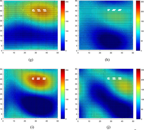
To illustrate the influence of the constraint on seismic inversion, we designed a contrast experiment which uses the same inversion parameters but without operations about the constraint:

1. Do not screen initial particles.

2. Set $D\equiv \text{1}$.

We conduct two additional experiments with the constraint and three experiments without the constraint and number them as 2–6 (the experiment conducted in Section 3.1 is numbered as 1), the inversion results are shown in Figure 5.

Figure 5. Inversion results obtained from contrast experiments. (a) Inversion result before stress change obtained from inversion Experiment 2 that has stress value change constraint. (b) Inversion result after stress change obtained from inversion Experiment 2 that has stress value change constraint. (c) Inversion result before stress change obtained from inversion Experiment 3 that has stress value change constraint. (d) Inversion result after stress change obtained from inversion Experiment 3 that has stress value change constraint. (e) Inversion result before stress change obtained from inversion Experiment 4 that has no stress value change constraint. (f) Inversion result after stress change obtained from inversion Experiment 4 that has no stress value change constraint. (g) Inversion result before stress change obtained from inversion Experiment 5 that has no stress value change constraint. (h) Inversion result after stress change obtained from inversion Experiment 5 that has no stress value change constraint. (i) Inversion result before stress change obtained from inversion Experiment 6 that has no stress value change constraint. (j) Inversion result after stress change obtained from inversion Experiment 6 that has no stress value change constraint.

Distance between inversion results and true wave velocity distributions and the variances of these distances are shown in Figure 6.

Figure 6. Distances and variances of these distances. (a) Distance between inversion results and true wave velocity distributions. (b) Variances of the distances.

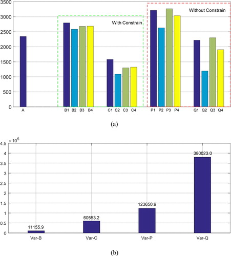
The meanings of the symbols in Figure 6 are shown in Table 2.

Table 2. Meanings of symbols in contrast experiment.

Symbol	Calculation method	Meaning
A	$\Vert mbD1+maD1-mb-ma{\Vert }_2$	Distance between frequency-domain-truncated true models and true models, the meanings of $mbD1$, $maD1$, $mb$ and $ma$ are same with the symbols in Table 1
B1,B2,B3	$\Vert r{b}_i+r{a}_i-mb-ma{\Vert }_2$ $i=1,2,3$	Distance between inversion results and true models, the subscript $i$ indicates the experiment number. Meanings of $rb$ and $ra$ are same with the symbols in Table 1
B4	$\frac{{\sum }_{i=1}^3{\Vert r{b}_i+r{a}_i-mb-ma\Vert }_2}{3}$	Mean distance between inversion results and true models
C1,C2,C3	$\Vert r{b}_i+r{a}_i-mbD1-maD1{\Vert }_2$ $i=1,2,3$	Distance between inversion results and frequency-domain-truncated true models
C4	$\frac{{\sum }_{i=1}^3{\Vert r{b}_i+r{a}_i-mbD1-maD1\Vert }_2}{3}$	Mean distance between inversion results and frequency-domain-truncated true models
P1,P2,P3	$\Vert r{b}_i+r{a}_i-mb-ma{\Vert }_2$ $i=4,5,6$	Distance between inversion results and true models
P4	$\frac{{\sum }_{i=4}^6{\Vert r{b}_i+r{a}_i-mb-ma\Vert }_2}{3}$	Mean distance between inversion results and true models
Q1,Q2,Q3	$\Vert r{b}_i+r{a}_i-mbD1-maD1{\Vert }_2$ $i=4,5,6$	Distance between inversion results and frequency-domain-truncated true models
Q4	$\frac{{\sum }_{i=4}^6{\Vert r{b}_i+r{a}_i-mbD1-maD1\Vert }_2}{3}$	Mean distance between inversion results and frequency-domain-truncated true models
Var-B	$\frac{{(B1-B4)}^2+{(B2-B4)}^2+{(B3-B4)}^2}{2}$	Variance of B1, B2 and B3
Var-C	$\frac{{(C1-C4)}^2+{(C2-C4)}^2+{(C3-C4)}^2}{2}$	Variance of C1, C2 and C3
Var-P	$\frac{{(P1-P4)}^2+{(P2-P4)}^2+{(P3-P4)}^2}{2}$	Variance of P1, P2 and P3
Var-Q	$\frac{{(Q1-Q4)}^2+{(Q2-Q4)}^2+{(Q3-Q4)}^2}{2}$	Variance of Q1, Q2 and Q3

As can be seen from Figure 6(a), the results obtained from inversion with stress change constraint are significantly better than those without the constraint. The mean distance between the results obtained from inversion with the constraint and true models (B4) is 2686.76 while the mean distance between the results obtained from the inversion without the constraint and true models (P4) is 3036.7. This indicates that the constraint brings an improvement of about 11.5% in the reliability of inversion results. Better than the improvement of the mean distance between the inversion results and the true models, the mean distances between inversion results and frequency-domain-truncated true models are 1322.5 (C4) and 1904.5 (Q4), respectively. Therefore, the improvement increases to 30.6% and indicates again that inversion results obtained from the new method proposed in this paper are closer to the frequency-domain-truncated true models with the same $D$ than true models.

The variances as shown in Figure 6(b) show the improvement of the stability of inversion results made by the constraint introduced in this paper. The constraint reduces the variance of the distances by about 91% (Var-B and Var-P) and 84.1% (Var-C and Var-Q), respectively, which indicate that whatever type of true models are compared to, the stress value change direction constraint greatly improves the stability of seismic inversion.

4. Conclusions and discussions

Both theoretic analyses and experimental results indicate that multi-parameter joint inversion is an effective way to reduce multiplicity of inversion when observation collections are insufficient. Based on this idea, we introduce stress value changes to constrain seismic inversion and successfully reduce the multiplicity in the inversion. Numerical experiments show that the new method proposed in this paper is convergent and reduces the mean distance between results obtained from inversions with the constraint and true models by about 11.5%, reduces the variance by about 91%, reduces the mean distance between results obtained from the inversion with the constraint and frequency-domain-truncated true models by about 30.6% and reduces the variance by about 84.1%. These results indicate that the reliability and stability of inversion with the constraint is better than the inversion without them, and provides a new idea for improving seismic inversion result in underground coal mine.

Acknowledgements

The authors are very grateful to the two reviewers, Dr Giuliana Rossi and Dr Wilson M. Figueiró, for their suggestions on the grammar and structure of this paper.

Data availability statement

All the computer codes are available at: https://github.com/feiyucq/Seismic-Tomography-with-Stress-Change-Direction-Constraint.git

Disclosure statement

No potential conflict of interest was reported by the author(s).

Additional information

Funding

This work was supported by the National Key R&D Program of China [grant number 2017YFC0804401] and Youth Foundation of Xuzhou Institute of Technology [grant number XKY2018222].

References

- Cai W, Dou L, Cao A, et al. Application of seismic velocity tomography in underground coal mines: a case study of Yima mining area, Henan, China. J Appl Geophys. 2014;109:140–149. doi: 10.1016/j.jappgeo.2014.07.021
- Rawlinson N, Fichtner A, Sambridge M, et al. Seismic tomography and the assessment of uncertainty. Adv Geophys. 2014;55:1–76. doi: 10.1016/bs.agph.2014.08.001
- Tikhotsky S, Achauer U. Inversion of controlled-source seismic tomography and gravity data with the self-adaptive wavelet parametrization of velocities and interfaces. Geophys J Int. 2008;172(2):619–630. doi: 10.1111/j.1365-246X.2007.03648.x
- Jean C, Sergey V, Guust N, et al. Global seismic tomography with sparsity constraints: comparison with smoothing and damping regularization. J Geophys Res-Solid Earth. 2013;118(9):4887–4899. doi: 10.1002/jgrb.50326
- Syracuse EM, Zhang H, Maceira M. Joint inversion of seismic and gravity data for imaging seismic velocity structure of the crust and upper mantle beneath Utah, United States. Tectonophysics. 2017;718:105–117. doi: 10.1016/j.tecto.2017.07.005
- Demirci İ, Dikmen Ü, Candansayar ME. Two-dimensional joint inversion of magnetotelluric and local earthquake data: discussion on the contribution to the solution of deep subsurface structures. Phys Earth Planet Inter. 2018;275:56–68. doi: 10.1016/j.pepi.2018.01.006
- Zhou Y, Zhao Z, Liu C, et al. Inversion analysis of crustal stress distribution law in gully geomorphic mining area. Geotech Geol Eng. 2019;37:4075–4087. doi: 10.1007/s10706-019-00894-1
- Zhang N, Zhang N, Han C, et al. Borehole stress monitoring analysis on advanced abutment pressure induced by Longwall Mining. Arab J Geosci. 2014;7(2):457–463. doi: 10.1007/s12517-013-0831-7
- Gong S-Y, Dou L-M, Xu X-J, et al.. Experimental study on the correlation between stress and P-wave velocity for burst tendency coal-rock samples. J Min Saf Eng. 2012;29(1):67–71.
- Donoho D L. Compressed sensing. IEEE Trans Inf Theory. 2006;52(4):1289–1306. doi: 10.1109/TIT.2006.871582
- Mallat S. A wavelet tour of signal processing: the sparse way. 3rd ed. Burlington (MA): Academic Press; 2008.
- Kennedy J, Eberhart RC. Particle swarm optimization. Proceedings of ICNN’95 – International Conference on Neural Networks; 1995 Nov. 27–Dec. 1; Perth, WA. IEEE; 2002. p. 1942–1948.
- Peng P, Wang L. 3DMRT: a computer Package for 3D model-based seismic wave Propagation. Seismol Res Lett. 2019;90(5):2039–2045.