Analytical solutions for some unsteady flows of fluids with linear dependence of viscosity on the pressure

Abstract

New exact solutions for unidirectional unsteady flows of incompressible viscous fluids with linear dependence of viscosity on the pressure between two infinite horizontal parallel plates are established when the lower plate is moving in its plane with an arbitrary time-dependent velocity. In addition to being useful solutions to idealizations of technologically relevant problems such exact solutions also serve to test the validity and the efficacy of numerical schemes that have been developed for much more complicated three-dimensional flows. The flows considered herein correspond to important solutions in the study of the classical Navier-Stokes fluid model. General results which are obtained can generate exact solutions for any motion of this type of the respective fluids. For illustration, three special cases with technical relevance are considered, and the variations of the fluid velocity and the non-trivial shear stress are graphically presented and discussed in some situations. The exact solutions corresponding to some motions generated by an accelerated plate are connected to the adequate solutions of the simple Couette flow.

KEYWORDS:

• Semi-inverse solutions
• pressure-dependent viscosity
• incompressible fluid
• parallel plates
• general solutions

2010 MATHEMATICS SUBJECT CLASSIFICATION:

• 76A05

1. Introduction

Semi-inverse solution techniques play a central role in mechanics. In using the semi-inverse approach, one seeks solutions of a particular class for the deformation or flow of the particular material under consideration. The forces (tractions) that are necessary to engender such a deformation or flow are computed a posteriori after a solution of the form sought has been determined. Of course, one is not guaranteed in finding solutions of the special form that is sought. Solutions in addition to those of the special form sought are also possible, especially when the full governing equations are non-linear. Most of the well-known exact solutions that are established in mechanics are semi-inverse solutions. Usually, semi-inverse solutions greatly simplify the governing equations thereby making these equations amenable to analysis. For instance, the governing non-linear partial differential equations may reduce to non-linear or even linear partial differential equations of lower order or to non-linear or linear ordinary differential equations.

An important class of semi-inverse solutions contains the universal solutions established within the context of non-linear elasticity (see Ericksen [1,2]) and those of simple materials (see Wineman [3], Carroll [4], Fosdick [5]). Universal solutions are solutions possible in every material that belongs to a certain class. The tractions necessary to produce the particular solution could be different from one class of materials to another. Such universal solutions accord the opportunity for carrying out experiments that correspond to the type of semi-inverse solution under consideration for every member belonging to the class. It may however be argued that one should not necessarily expect a specific deformation or flow to be possible in every member belonging to the class. But such an argument does not impugn the general semi-inverse technique as one can seek solutions of a general form rather than a specific form. This would then imply that the structure of the solution can change from material to material.

In this paper we shall illustrate the power of the semi-inverse technique by studying the flows of fluids with pressure dependent viscosity. Very few exact solutions are available for flows of such fluids. We will find that the semi-inverse technique allows us to find solutions in certain situations while it fails to deliver solutions in other circumstances. More precisely, we establish general exact solutions for motions of fluids with linear dependence of viscosity on the pressure between two infinite horizontal parallel plates. These solutions, which are obtained using a suitable change of the independent variable and the finite Hankel transform, can be used to provide exact solutions for any motion of this type of respective fluids. Finally, for illustration, three special classes of motions are considered and the variations of velocity and shear stress fields in different circumstances are graphically underlined and discussed. Furthermore, for validation, the steady-state solutions for oscillating motions and the simple Couette flow are presented in different forms whose equivalence is graphically proved.

2. The model

That the viscosity of a fluid could depend on the normal stresses (pressure) was recognized by Stokes [6]. In liquids, while the density might vary by a very small value, say a few percents, the viscosity may vary by orders of magnitude (as much as a factor of $\text{1}{\text{0}}^{\text{8}}$). Thus, it might be reasonable to model such fluids with a pressure dependent viscosity. There has been a great deal of research concerning the dependence of the viscosity on the pressure. The literature related to such work prior to 1931 can be found in the treatise by Bridgman on the Physics of high pressure [7]. There have been recent experiments by Cutler et al. [8], Griest et al. [9], Johnson and Cameron [10], Johnson and Greenwood [11], Johnson and Tevaarwerk [12], Bain and Winer [13], which confirm the strong dependence of viscosity on the pressure.

Rigorous mathematical studies have been carried out concerning the existence and uniqueness of the solutions to the equations governing the flows of fluids with pressure dependent viscosity (see Malek et al. [14,15], Hron et al. [16], Franta et al. [17]). These mathematical studies are for the full partial differential equations; certain special subclasses of flows are also studied. Hron et al. [16] sought unidirectional semi-inverse solutions and showed that such solutions were possible only under special circumstances. Here, we consider yet another class of semi-inverse solutions to the flows of a fluid with linear dependence of the viscosity on the pressure.

During the flows of fluids with pressure dependent viscosity, it is possible for concentrations of vorticity to occur adjacent to solid boundaries, and at times even in the interior of the flow, at low Reynolds number (see Rajagopal [18,19]). These earlier studies pertain to steady flows of the fluid, and it would be interesting to investigate the formation and the evolution of such layers within the context of unsteady flows. The classes of semi-inverse solutions that are sought have the appropriate structure to investigate this issue.

We shall consider the flows of an incompressible fluid whose Cauchy stress has the form (1) $\mathit{T}=-p\mathit{I}+\mu (p){\mathit{A}}_1,$(1) where $-p\mathit{I}$ denotes the indeterminate part of the stress due to the constraint of incompressibility, and $\mu (p)$ denotes the viscosity that depends on the pressure p. The tensor ${\mathit{A}}_1$is given by (2) ${\mathit{A}}_1=\left[\left(\frac{\mathrm{\partial }\mathit{v}}{\mathrm{\partial }\mathit{x}}\right)+{\left(\frac{\mathrm{\partial }\mathit{v}}{\mathrm{\partial }\mathit{x}}\right)}^T\right],$(2) where $\mathit{v}$ denotes the velocity field. Since the fluid is incompressible, it can only undergo isochoric motions, and thus the velocity field $\mathit{v}$ must satisfy the constraint (3) $\text{div}\mathit{v}=0.$(3) On substituting (1) into the balance of linear momentum (4) $\text{div}\mathit{T}+\rho \mathit{b}=\rho \frac{d\mathit{v}}{dt},$(4) where $\rho$ is the density of the fluid and b the external body force, and making use of (2) and (3), we find the following (5) $-\text{grad}p+\mu (p)\mathrm{\Delta }\mathit{v}+{\mathit{A}}_{\text{1}}[\text{grad}\mu ]+\rho \mathit{b}=\rho \frac{d\mathit{v}}{dt}.$(5) 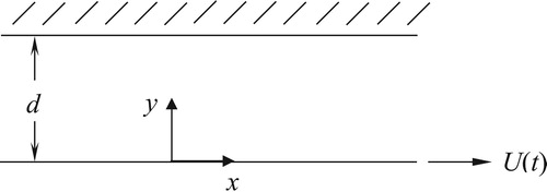We are interested in finding semi-inverse solutions for flows taking place in the domain between two infinite horizontal parallel plates due to unsteady motions of the lower plate which is situated in the plane $y=0$ of a fixed Cartesian coordinate system x, y and z. Thus, we will seek unsteady unidirectional solutions of the form (6) $\mathit{v}=u\text{(}y,t\text{)}\mathit{i},p=p(y,t),$(6) where i is the unit vector along the x-coordinate direction. This flow is depicted in Figure 1.

Figure 1. Illustration of the flow for the boundary value problem under consideration.

We notice that the form of the velocity field that has been chosen automatically satisfies the incompressibility constraint (3). On substituting (6) into (5), we obtain (7) $\frac{\mathrm{\partial }}{\mathrm{\partial }y}\left[\mu (p)\frac{\mathrm{\partial }u}{\mathrm{\partial }y}\right]=\rho \frac{\mathrm{\partial }u}{\mathrm{\partial }t},\frac{\mathrm{\partial }p}{\mathrm{\partial }y}+\rho g=0,$(7) because $\mathit{b}=-g\mathit{j}\text{,}\mathit{j}$ being the unit vector along the y-coordinate direction while g is the acceleration due to gravity.

It follows from (7)₂ and (6)₂ that (8) $p=p(y,t)=-\rho gy+f(t),$(8) where $f(t)$ is an arbitrary function of t. The equation (7)₁ becomes (9) ${\mu }^{\mathrm{\prime }}(p)\frac{\mathrm{\partial }p}{\mathrm{\partial }y}\frac{\mathrm{\partial }u}{\mathrm{\partial }y}+\mu (p)\frac{{\mathrm{\partial }}^{2}u}{\mathrm{\partial }{y}^2}=\rho \frac{\mathrm{\partial }u}{\mathrm{\partial }t}.$(9) Thus, we seek a solution to Eq. (9) subjected to appropriate initial and boundary conditions. More exactly we are looking for solutions of this equation for the linear dependence of viscosity on the pressure, namely when (10) $\mu (p)=\alpha p,\alpha >0.$(10) The first exact solutions for the steady flow of such fluids between infinite parallel plates which are moving in their planes with a constant speed seem to be those obtained by Hron et al. [20]. Other interesting results for the same steady flow have been established by Rajagopal [21,22] for linear, power law or exponential dependence of viscosity on the pressure. In the second paper the flow down an inclined plane due to gravity and the Poiseuille flow between parallel plates in the absence of gravity have been analytically investigated. Some numerical solutions, but in the non-steady case, have been developed by Massoudi and Phuoc [23] and Srinivasan and Rajagopal [24]. Exact solutions, in terms of Kelvin functions, have been determined by Prusa [25] for the modified Stokes problems corresponding to incompressible Newtonian fluids with linear and exponential dependence of viscosity on the pressure. General solutions for the same problems in terms of a suitable system of eigenfunctions and eigenvalues, as well as qualitative and uniqueness results, have been established by Rajagopal et al. [26]. As even steady unidirectional flows are generally not possible for the power-law case corresponding to physically meaningful problems (see Hron et al. [16]), we cannot necessarily expect to obtain solutions for unidirectional unsteady flows. Further, a simpler sub-class of semi-inverse solutions can we sought. We should however recognize such special forms of solutions might not exist. Here, let us consider a pressure field wherein $f(t)$ is constant. Thus (11) $p(y,t)=p(y)=\rho g(d-y)+p_d,$(11) where $p_d=p(d)$ and d is the distance between plates.

3. Flow induced by the lower plate that is moving in its plane

Let us consider an incompressible viscous fluid with linear dependence of the viscosity on the pressure at rest between two infinite horizontal parallel plates at a distance d apart. At time $t=0^{+}$, the lower plate begins to move with a time-dependent velocity $U(t)=Uh(t)$ in a parallel direction to the upper one, which is stationary. Here U is a constant velocity while the function $h(\cdot )$ is piecewise continuous and $h(0)=0$. The fluid is gradually moved, and we are looking for a velocity field of the form (6)₁. The continuity equation is identically satisfied, and the balance of momentum reduces to Eq. (9).

Introducing $\mu (p)=\alpha p=\alpha [\rho g(d-y)+p_d]$ in Eq. (9), we find that (12) $\alpha [\rho g(d-y)+p_d]\frac{{\mathrm{\partial }}^{2}u(y,t)}{\mathrm{\partial }{y}^2}-\alpha \rho g\frac{\mathrm{\partial }u(y,t)}{\mathrm{\partial }y}=\rho \frac{\mathrm{\partial }u(y,t)}{\mathrm{\partial }t};0<y<d,t>0.$(12) The corresponding initial and boundary conditions are (13) $\begin{array}{rl}& u(y,0)=0;0\le y\le d,\end{array}$(13) (14) $\begin{array}{rl}& u(0,t)=Uh(t),u(d,t)=0;t>0,\end{array}$(14) while the non-trivial shear stress $\tau (y,t)$, as it results from Eqs. (1), (10) and (11), is given by (15) $\tau (y,t)=\alpha [\rho g(d-y)+p_d]\frac{\mathrm{\partial }u(y,t)}{\mathrm{\partial }y}.$(15) In order to make non-dimensional this problem, we introduce following dimensionless variables and functions (16) $y^{\ast }=\frac{y}{d},t^{\ast }=\frac{\alpha g}{d}t,u^{\ast }=\frac{u}{U},{\tau }^{\ast }=\frac{\tau }{\alpha \rho gU},$(16) Introducing Eqs. (16) in (12)–(14) and dropping out the star notation, we find the next dimensionless initial and boundary value problem (17) $\begin{array}{rl}& (1-y+\beta )\frac{{\mathrm{\partial }}^{2}u(y,t)}{\mathrm{\partial }{y}^2}-\frac{\mathrm{\partial }u(y,t)}{\mathrm{\partial }y}=\frac{\mathrm{\partial }u(y,t)}{\mathrm{\partial }t};0<y<1,t>0,\end{array}$(17) (18) $\begin{array}{rl}& u(y,0)=0;0\le y\le 1,\end{array}$(18) (19) $\begin{array}{rl}& u(0,t)=h(t),u(1,t)=0;t>0,\end{array}$(19) where $\beta =\frac{p_d}{\rho gd}$ is the non-dimensional pressure The dimensionless non-trivial shear stress $\tau (y,t)$ will be given by (20) $\tau (y,t)=(1-y+\beta )\frac{\mathrm{\partial }u(y,t)}{\mathrm{\partial }y};0<y<1,t>0.$(20) To solve the partial differential equation (17) with the initial and boundary conditions (18) and (19), we firstly make the change of independent variable (21) $y=1+\beta -\frac{r^2}{4}\text{or}r=2\sqrt{1-y+\beta }.$(21) Using (21)₁, our problem reduces to the partial differential equation (22) $\frac{{\mathrm{\partial }}^{2}u(r,t)}{\mathrm{\partial }{r}^2}+\frac{1}{r}\frac{\mathrm{\partial }u(r,t)}{\mathrm{\partial }r}=\frac{\mathrm{\partial }u(r,t)}{\mathrm{\partial }t};a<r<b,t>0,$(22) with the initial and boundary conditions (23) $\begin{array}{rl}& u(r,0)=0;a\le r\le b,\end{array}$(23) (24) $\begin{array}{rl}& u(a,t)=0,u(b,t)=h(t);t>0,\end{array}$(24) where $a=2\sqrt{\beta }$ and $b=2\sqrt{1+\beta }$.

Let us now consider the suitable change of unknown function (25) $u(r,t)=v(r,t)+\frac{r-a}{b-a}h(t).$(25) Replacing $u(r,t)$ in (22)-(24), we obtain the following initial and boundary value problem (26) $\begin{array}{rl}& \frac{{\mathrm{\partial }}^{2}v(r,t)}{\mathrm{\partial }{r}^2}+\frac{1}{r}\frac{\mathrm{\partial }v(r,t)}{\mathrm{\partial }r}+\frac{h(t)-r(r-a)h^{\mathrm{\prime }}(t)}{r(b-a)}=\frac{\mathrm{\partial }v(r,t)}{\mathrm{\partial }t};a<r<b,t>0,\end{array}$(26) (27) $\begin{array}{rl}& v(r,0)=0;a\le r\le b,\end{array}$(27) (28) $\begin{array}{rl}& v(a,t)=v(b,t)=0;t>0.\end{array}$(28)

In order to solve this problem, we use the finite Hankel transform. Consequently, multiplying Eq. (26) by $rA(r,r_n)$, where (29) $A(r,r_n)=Y_0(a{r}_n)J_0(r{r}_n)-J_0(a{r}_n)Y_0(r{r}_n)$(29) and $J_0(\cdot )$ and $Y_0(\cdot )$ are standard Bessel functions, integrating the result with respect to r from a to b and bearing in mind the conditions (27) and (28) and the known result [27] (30) ${\int }_a^{b}rA(r,r_n)\left[\frac{{\mathrm{\partial }}^{2}v(r,t)}{\mathrm{\partial }{r}^2}+\frac{1}{r}\frac{\mathrm{\partial }v(r,t)}{\mathrm{\partial }r}\right]dr=\frac{2}{\pi }\left[v(b,t)\frac{J_0(a{r}_n)}{J_0(b{r}_n)}-v(a,t)\right]-r_n^2{v}_{Hn}(t),$(30) we find that (31) $\begin{array}{rl}& {\dot{v}}_{Hn}(t)+r_n^2{v}_{Hn}(t)=c_n(t);t>0,n=1,2,3,\dots \end{array}$(31) (32) $\begin{array}{rl}& v_{Hn}(0)=0;n=1,2,3,\dots \end{array}$(32) Into above relations (33) $v_{Hn}(t)={\int }_a^{b}rv(r,t)A(r,r_n)dr;n=1,2,3,\dots ,$(33) is the finite Hankel transform of the function $v(r,t)$ and $r_n$ are the positive roots of the transcendental equation (34) $\begin{array}{rl}A(b,r)& =J_0(br)Y_0(ar)-J_0(ar)Y_0(br)=0\text{and}\end{array}$(34) (35) $\begin{array}{rl}{c}_n(t)& =\frac{1}{b-a}[a_{n}h(t)-b_n{h}^{\mathrm{\prime }}(t)];a_n={\int }_a^{b}A(r,r_n)dr\text{and}\\ b_n& ={\int }_a^{b}r(r-a)A(r,r_n)dr.\end{array}$(35) Solving the ordinary differential equation (31) with the initial condition (32) and applying the inverse Hankel transform to the result, we obtain (see [27], the page 482) (36) $v(r,t)=\frac{{\pi }^2}{2}\sum _{n=1}^{\mathrm{\infty }}\frac{r_n^2{J}_0^2(b{r}_n)A(r,r_n)}{J_0^2(a{r}_n)-J_0^2(b{r}_n)}{\int }_0^t{c}_n(s){\text{e}}^{-r_n^2(t-s)}ds,$(36) where the sum extends over all positive roots of the equation (34).

Now, introducing Eq. (36) in (25) and coming back to the initial variable y, we find for the velocity field $u(y,t)$ the expression (37) $\begin{array}{rl}u(y,t)& =\frac{\sqrt{1-y+\beta }-\sqrt{\beta }}{\sqrt{1+\beta }-\sqrt{\beta }}h(t)\\ & +\frac{{\pi }^2}{2}\sum _{n=1}^{\mathrm{\infty }}\frac{r_n^2{J}_0^2(b{r}_n)}{J_0^2(a{r}_n)-J_0^2(b{r}_n)}A(2\sqrt{1-y+\beta },r_n){\int }_0^t{c}_n(s){\text{e}}^{-r_n^2(t-s)}ds,\end{array}$(37) where $c_n(t)$ is defined by Eq. (35)₁. A simple analysis clearly shows that $u(y,t)$ given by Eq. (37) satisfies all imposed initial and boundary conditions.

Adequate non-trivial shear stress, as it results from equations (20) and (37), is given by (38) $\begin{array}{rl}\tau (y,t)& =-\frac{1}{2}\frac{\sqrt{1-y+\beta }}{\sqrt{1+\beta }-\sqrt{\beta }}h(t)-\frac{{\pi }^2}{2}\sqrt{1-y+\beta }\sum _{n=1}^{\mathrm{\infty }}\frac{r_n^3{J}_0^2(b{r}_n)}{J_0^2(a{r}_n)-J_0^2(b{r}_n)}\\ & \times B(2\sqrt{1-y+\beta },r_n){\int }_0^t{c}_n(s){\text{e}}^{-r_n^2(t-s)}ds,\end{array}$(38) where $B(r,r_n)=J_0(a{r}_n)Y_1(r{r}_n)-Y_0(a{r}_n)J_1(r{r}_n)$.

The general expressions (37) and (38) for the fluid velocity and the non-trivial shear stress, respectively, can generate exact solutions for any motion with technical relevance of this type using suitable selections of the function $h(\cdot )$. The frictional forces per unit area exerted by the fluid on the two plates are immediately obtained taking $y=0$ or $y=1$ in Eq. (38). For illustration, as well as to get some physical insight of results that have been obtained, three important cases with engineering applications will be here considered.

3.1. Case $h(t)=H(t)$ (Simple Couette flow)

The flow between two infinite parallel plates induced by one of them that is moving in its plane with a constant velocity is called the simple Couette flow [28]. Substituting h(t) by H(t) (the Heaviside unit step function) in equations (37) and (38), we find the dimensionless starting solutions corresponding to this motion, namely (39) $\begin{array}{rl}{u}_C(y,t)& =\frac{\sqrt{1-y+\beta }-\sqrt{\beta }}{\sqrt{1+\beta }-\sqrt{\beta }}H(t)+\frac{{\pi }^2}{2(b-a)}H(t)\\ & \times \sum _{n=1}^{\mathrm{\infty }}\frac{J_0^2(b{r}_n)A(2\sqrt{1-y+\beta },r_n)}{J_0^2(a{r}_n)-J_0^2(b{r}_n)}[a_n-(a_n+b_n{r}_n^2){\text{e}}^{-r_n^{2}t}],\end{array}$(39) (40) $\begin{array}{rl}{\tau }_C(y,t)& =-\frac{1}{2}\frac{\sqrt{1-y+\beta }}{\sqrt{1+\beta }-\sqrt{\beta }}H(t)-\frac{{\pi }^2\sqrt{1-y+\beta }}{2(b-a)}H(t)\\ & \times \sum _{n=1}^{\mathrm{\infty }}\frac{r_n{J}_0^2(b{r}_n)B(2\sqrt{1-y+\beta },r_n)}{J_0^2(a{r}_n)-J_0^2(b{r}_n)}[a_n-(a_n+b_n{r}_n^2){\text{e}}^{-r_n^{2}t}].\end{array}$(40) In order to obtain the solutions (39) and (40), we also used the fact that $H^{\mathrm{\prime }}(t)=\delta (t)$ (the Dirac delta function) and (41) ${\int }_0^t\delta (s)f(t-s)ds={\int }_0^t\delta (t-s)f(s)ds=f(t).$(41) By now making $t\to \mathrm{\infty }$ into Eqs. (39) and (40), the steady (permanent or long time) solutions (42) $\begin{array}{rl}{u}_{Cp}(y)& =\frac{\sqrt{1-y+\beta }-\sqrt{\beta }}{\sqrt{1+\beta }-\sqrt{\beta }}+\frac{{\pi }^2}{2(b-a)}\sum _{n=1}^{\mathrm{\infty }}\frac{a_n{J}_0^2(b{r}_n)}{J_0^2(a{r}_n)-J_0^2(b{r}_n)}A(2\sqrt{1-y+\beta },r_n),\end{array}$(42) (43) $\begin{array}{rl}{\tau }_{Cp}(y)& =-\frac{1}{2}\frac{\sqrt{1-y+\beta }}{\sqrt{1+\beta }-\sqrt{\beta }}-\frac{{\pi }^2\sqrt{1-y+\beta }}{2(b-a)}\\ & \times \sum _{n=1}^{\mathrm{\infty }}\frac{a_n{r}_n{J}_0^2(b{r}_n)}{J_0^2(a{r}_n)-J_0^2(b{r}_n)}B(2\sqrt{1-y+\beta },r_n),\end{array}$(43) are obtained. 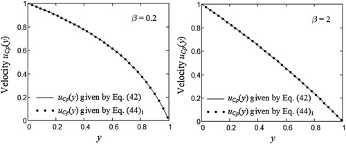Direct computations show that the steady solutions (42) and (43) can be also presented in the equivalent but simpler forms (44) $u_{Cp}(y)=\ln \left(\frac{1-y+\beta }{\beta }\right)/\ln \left(\frac{1+\beta }{\beta }\right),{\tau }_{Cp}=-1/\ln \left(\frac{1+\beta }{\beta }\right).$(44) These solutions are independent of the initial condition, but they satisfy the corresponding governing equations and the boundary conditions. The equivalence of the steady solutions (42) and (44)₁ is graphically illustrated by Figure 2. As regards Eq. (44)₂, contrary to our expectations, the steady shear stress corresponding to this motion is constant on the whole flow domain although the fluid velocity is a function of y. Furthermore, this shear stress in absolute value is an increasing function with respect to the non-dimensional pressure $\beta$.

Figure 2. Profiles of steady component $u_{Cp}(y)$ of $u_C(y,t)$ given by equations (42) and (44)₁ for two different values of $\beta$.

3.2. Case $h(t)=t^{\gamma },(\gamma >0)$ (Flow due to an accelerated plate)

By substituting $h(t)$ by $t^{\gamma }$ in equations (37) and (38) we find the solutions (45) $\begin{array}{rl}{u}_{\gamma }(y,t)& =\frac{\sqrt{1-y+\beta }-\sqrt{\beta }}{\sqrt{1+\beta }-\sqrt{\beta }}{t}^{\gamma }+\frac{{\pi }^2}{2(b-a)}\sum _{n=1}^{\mathrm{\infty }}\frac{r_n^2{J}_0^2(b{r}_n)}{J_0^2(a{r}_n)-J_0^2(b{r}_n)}\\ & \times A(2\sqrt{1-y+\beta },r_n){\int }_0^t{s}^{\gamma -1}(a_{n}s-b_n\gamma \text{)}{\text{e}}^{-r_n^2(t-s)}ds,\end{array}$(45) (46) $\begin{array}{rl}{\tau }_{\gamma }(y,t)& =-\frac{1}{2}\frac{\sqrt{1-y+\beta }}{\sqrt{1+\beta }-\sqrt{\beta }}{t}^{\gamma }-\frac{{\pi }^2\sqrt{1-y+\beta }}{2(b-a)}\sum _{n=1}^{\mathrm{\infty }}\frac{r_n^3{J}_0^2(b{r}_n)}{J_0^2(a{r}_n)-J_0^2(b{r}_n)}\\ & \times B(2\sqrt{1-y+\beta },r_n){\int }_0^t{s}^{\gamma -1}(a_{n}s-b_n\gamma \text{)}{\text{e}}^{-r_n^2(t-s)}ds,\end{array}$(46) Corresponding to the motion of a fluid with linear dependence of the viscosity on the pressure induced by a slowly $(\gamma <1)$, constantly $(\gamma =1)$ or quickly $(\gamma >1)$ accelerating plate. This is an unsteady motion and remains unsteady. Of interest for us are the solutions corresponding to the motion due to a constantly accelerating plate, namely (47) $\begin{array}{rl}{u}_1(y,t)& =\frac{\sqrt{1-y+\beta }-\sqrt{\beta }}{\sqrt{1+\beta }-\sqrt{\beta }}t+\frac{{\pi }^2}{2(b-a)}\sum _{n=1}^{\mathrm{\infty }}\frac{J_0^2(b{r}_n)A(2\sqrt{1-y+\beta },r_n)}{J_0^2(a{r}_n)-J_0^2(b{r}_n)}\\ & \times \left[a_n\left(t-\frac{1-{\text{e}}^{-r_n^{2}t}}{r_n^2}\right)-b_n(1-{\text{e}}^{-r_n^{2}t})\right],\end{array}$(47) (48) $\begin{array}{rl}{\tau }_1(y,t)& =-\frac{1}{2}\frac{\sqrt{1-y+\beta }}{\sqrt{1+\beta }-\sqrt{\beta }}t-\frac{{\pi }^2\sqrt{1-y+\beta }}{2(b-a)}\sum _{n=1}^{\mathrm{\infty }}\frac{r_n{J}_0^2(b{r}_n)B(2\sqrt{1-y+\beta },r_n)}{J_0^2(a{r}_n)-J_0^2(b{r}_n)}\\ & \times \left[a_n\left(t-\frac{1-{\text{e}}^{-r_n^{2}t}}{r_n^2}\right)-b_n(1-{\text{e}}^{-r_n^{2}t})\right].\end{array}$(48) In order to bring to light the theoretical and practical importance of the solutions $u_C(y,t)$ and ${\tau }_C(y,t)$ corresponding to the simple Couette flow, we mention the fact that (49) $u_1(y,t)={\int }_0^t{u}_C(y,s)ds,{\tau }_1(y,t)={\int }_0^t{\tau }_C(y,s)ds.$(49) Furthermore, it is not difficult to show that for $\gamma =n$ (a natural number) (50) $\begin{array}{r}{u}_n(y,t)=(n!){\int }_0^t{\int }_0^{s_1}{\int }_0^{s_2}\dots {\int }_0^{s_{n-1}}{u}_C(y,s_n)d{s}_{n}d{s}_{n-1}\dots d{s}_1,\\ {\tau }_n(y,t)=(n!){\int }_0^t{\int }_0^{s_1}{\int }_0^{s_2}\dots {\int }_0^{s_{n-1}}{\tau }_C(y,s_n)d{s}_{n}d{s}_{n-1}\dots d{s}_1.\end{array}$(50) Consequently, knowing the solutions $u_C(y,t)$ and ${\tau }_C(y,t)$ corresponding to the simple Couette flow, we can determine by simple or multiple integrals the similar solutions for a large class of motions induced by an accelerated plate whose velocity is $U{t}^{n}H(t)$.

3.3. Case $h(t)=H(t)\cos (\omega t)\text{or}H(t)\sin (\omega t)$ (Flow due to an oscillating plate)

Replacing $h(t)$ by $H(t)\cos (\omega t)$or $H(t)\sin (\omega t)$ in equations (37) and (38) and using again the property (41), we find the starting solutions $u_c(y,t)$ and $u_s(y,t)$ corresponding to motions due to cosine or sine oscillations, respectively, of the lower plate. These solutions can be written as sums of steady-state (permanent) and transient components, that is (51) $u_c(y,t)=[u_{cp}(y,t)+u_{ct}(y,t)]H(t);u_s(y,t)=[u_{sp}(y,t)+u_{st}(y,t)]H(t),$(51) where (52) $\begin{array}{rl}{u}_{cp}(y,t)& =\frac{\sqrt{1-y+\beta }-\sqrt{\beta }}{\sqrt{1+\beta }-\sqrt{\beta }}\cos (\omega t)+\frac{{\pi }^2}{2(b-a)}\sum _{n=1}^{\mathrm{\infty }}\frac{r_n^2{J}_0^2(b{r}_n)A(2\sqrt{1-y+\beta },r_n)}{J_0^2(a{r}_n)-J_0^2(b{r}_n)}\\ & \times \left\{\frac{a_n{r}_n^2-b_n{\omega }^2}{r_n^4+{\omega }^2}\cos (\omega t)+\omega \frac{a_n+b_n{r}_n^2}{r_n^4+{\omega }^2}\sin (\omega t)\right\},\end{array}$(52) (53) $\begin{array}{rl}{u}_{ct}(y,t)& =-\frac{{\pi }^2}{2(b-a)}\sum _{n=1}^{\mathrm{\infty }}\frac{r_n^4{J}_0^2(b{r}_n)A(2\sqrt{1-y+\beta },r_n)}{J_0^2(a{r}_n)-J_0^2(b{r}_n)}\frac{a_n+b_n{r}_n^2}{r_n^4+{\omega }^2}{\text{e}}^{-r_n^{2}t},\end{array}$(53) (54) $\begin{array}{rl}{u}_{sp}(y,t)& =\frac{\sqrt{1-y+\beta }-\sqrt{\beta }}{\sqrt{1+\beta }-\sqrt{\beta }}\sin (\omega t)+\frac{{\pi }^2}{2(b-a)}\sum _{n=1}^{\mathrm{\infty }}\frac{r_n^2{J}_0^2(b{r}_n)A(2\sqrt{1-y+\beta },r_n)}{J_0^2(a{r}_n)-J_0^2(b{r}_n)}\\ & \times \left\{\frac{a_n{r}_n^2-b_n{\omega }^2}{r_n^4+{\omega }^2}\sin (\omega t)-\omega \frac{a_n+b_n{r}_n^2}{r_n^4+{\omega }^2}\cos (\omega t)\right\},\end{array}$(54) (55) $\begin{array}{rl}{u}_{st}(y,t)& =\frac{{\pi }^2\omega }{2(b-a)}\sum _{n=1}^{\mathrm{\infty }}\frac{r_n^4{J}_0^2(b{r}_n)A(2\sqrt{1-y+\beta },r_n)}{J_0^2(a{r}_n)-J_0^2(b{r}_n)}\frac{a_n+b_n{r}_n^2}{r_n^4+{\omega }^2}{\text{e}}^{-r_n^{2}t}.\end{array}$(55)

The corresponding shear stresses can be immediately obtained introducing the above solutions in equation (20). As it was to be expected, by making the oscillations’ frequency $\omega \to 0$ in equation (51)_1, we recover the solution (39) corresponding to the simple Couette flow.

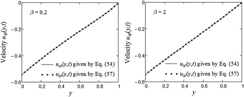
Following the same line as in [29, Section 3] it is not difficult to show that the steady-state components $u_{cp}(y,t)$ and $u_{sp}(y,t)$ of $u_c(y,t)$, respectively $u_s(y,t)$ can be also written in the simpler forms (56) $\begin{array}{rl}{u}_{cp}(y,t)& =Re\left\{\frac{K_0(a\sqrt{i\omega })I_0(2\sqrt{i\omega (1-y+\beta )})-I_0(a\sqrt{i\omega })K_0(2\sqrt{i\omega (1-y+\beta )})}{I_0(b\sqrt{i\omega })K_0(a\sqrt{i\omega })-I_0(a\sqrt{i\omega })K_0(b\sqrt{i\omega })}{\text{e}}^{i\omega t}\right\},\end{array}$(56) (57) $\begin{array}{rl}{u}_{sp}(y,t)& =\mathrm{Im}\left\{\frac{K_0(a\sqrt{i\omega })I_0(2\sqrt{i\omega (1-y+\beta )})-I_0(a\sqrt{i\omega })K_0(2\sqrt{i\omega (1-y+\beta )})}{I_0(b\sqrt{i\omega })K_0(a\sqrt{i\omega })-I_0(a\sqrt{i\omega })K_0(b\sqrt{i\omega })}{\text{e}}^{i\omega t}\right\},\end{array}$(57) where ‘Re’ and ‘Im’ denote the real and the imaginary parts, respectively, of that which follows.

Generally, the steady-state components of starting solutions are important for those who want to eliminate the transients from their experiments. More exactly, in practice it is necessary to know the time after which the fluid flows according to the steady-state solutions. This is the time after which the diagrams of starting solutions are almost identical to those of their corresponding steady-state components. It can be graphically determined if both the starting solutions and their steady-state components are known. Figures 3 and 4 clearly show the equivalence of the expressions (52) and (56), respectively (54) and (57) corresponding to the steady-state components $u_{cp}(y,t)$ and $u_{sp}(y,t)$ of staring solutions $u_c(y,t)$, respectively $u_s(y,t)$. This can be a certainty of our results’ correctness.

Figure 3. Profiles of the steady-state component $u_{cp}(y,t)$ of $u_c(y,t)$ given by equations (52) and (56) for two different values of $\beta$ and $t=10$.

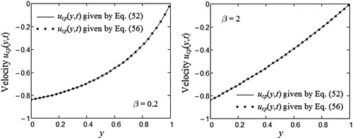
Figure 4. Profiles of the stead-state component $u_{sp}(y,t)$ of $u_s(y,t)$ given by equations (54) and (57) for two different values of $\beta$ and $t=10$.

4. Numerical results and conclusions

The unsteady motion of incompressible viscous fluids with linear dependence of viscosity on the pressure through a horizontal channel that is bounded by two infinite parallel plates is analytically studied when the lower plate is moving in its plane with an arbitrary time-dependent velocity $Uh(t)$ while the upper one is stationary. General exact expressions are established for the dimensionless fluid velocity $u(y,t)$ and the adequate non-trivial shear-stress $\tau (y,t)$. These expressions, that have been obtained using a suitable transform of the independent variable and the finite Hankel transform, satisfy all imposed initial and boundary conditions and can generate exact solutions for any motion with technical relevance of this type of the fluids in consideration.

For illustration, three special cases with technical relevance and engineering applications have been considered and the solutions corresponding to oscillatory motions and the simple Couette flow are presented as sum of steady-state and transient components. It was found that the steady component of the nontrivial shear stress ${\tau }_{Cp}$, corresponding to the simple Couette flow, is constant on the whole flow domain although the adequate component of velocity $u_{Cp}$ is a function of y. Furthermore, for validation, the steady-state components $u_{Cp}(y),u_{cp}(y,t)$ and $u_{sp}(y,t)$ corresponding to the simple Couette flow and the oscillating motions are presented in different forms whose equivalence is graphically proved in Figures 2–4. In addition, as it was to be expected, the velocity field $u_C(y,t)$ can be obtained as a limiting case of the solution $u_c(y,t)$ when the oscillations’ frequency $\omega \to 0$.

It is worth pointing out the fact that the structure of present solutions is completely different of that of Prusa [25] or Rajagopal et al. [26] solutions. Furthermore, they are presented in simple forms, and the dimensionless solutions corresponding to some motions induced by an accelerated plate (that is moving in its plane with a velocity given by $U{t}^{n}H(t)$ with n a natural number) are connected to the similar solutions of the simple Couette flow by Eqs. (50). More exactly, these solutions are obtained as simple or multiple integrals of the solutions $u_C(y,t)$ and ${\tau }_C(y,t)$ of the simple Couette flow.

In order to bring to light some physical insight of results that have been obtained, Figures 5–14 are depicted at three values of the dimensionless pressure $\beta$. Figures 5 and 6 illustrate the development of the dimensionless velocity profiles corresponding to a unit step increase in the boundary velocity given by Eq. (39). The solution is evaluated at three representative $\beta$ values at $t=0.1$ and $t=1$. The fluid velocity, as expected, smoothly decreases from the maximum value 1 on the moving plate up to the zero value on the stationary plate. At small values of the time t, as it results from Figure 5, the fluid velocity is an increasing function with respect to $\beta$ on the entire flow domain. An opposite trend appears after a critical value of the time t greater than 0.1.

Figure 5. Velocity profiles corresponding to a unit step increase in boundary velocity, given by equation (39), evaluated at three different $\beta$ values at $t=0.1$.

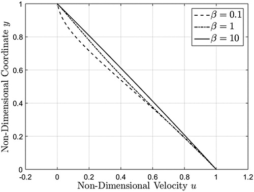
Figure 6. Velocity profiles corresponding to a unit step increase in boundary velocity, given by equation (39), evaluated at three different $\beta$ values at $t=1$.

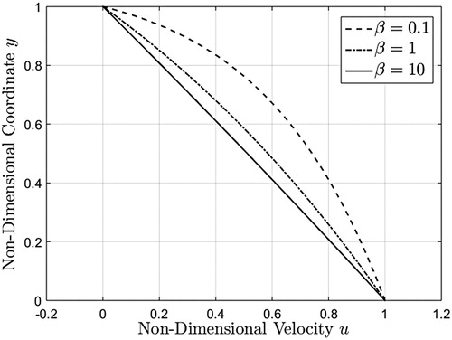
Figure 7. Shear stress profiles corresponding to a unit step increase in boundary velocity, given by equation (40), evaluated at three different $\beta$ values at $t=0.1$.

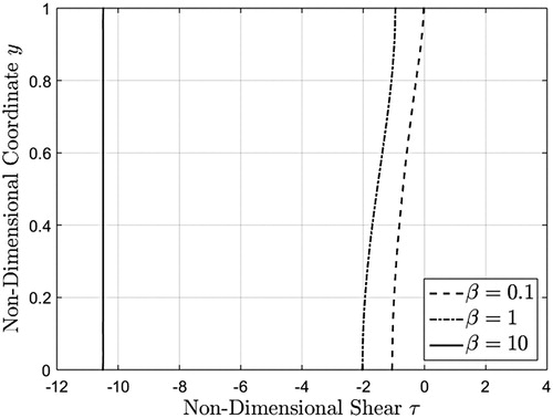
Figure 8. Shear stress profiles corresponding to a unit step increase in boundary velocity, given by equation (40), evaluated at three different $\beta$ values at $t=1$.

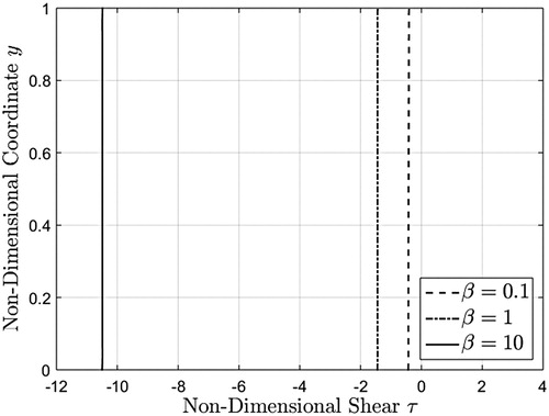
Figure 9. Midplane velocity as a function of time corresponding to a unit step increase in boundary velocity, given by equation (39), evaluated at three different $\beta$ values.

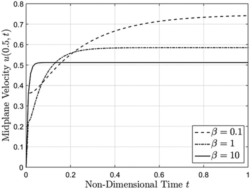
Figure 10. Lower wall shear stress as a function of time corresponding to a unit step increase in boundary velocity, given by equation (40), evaluated at three different $\beta$ values.

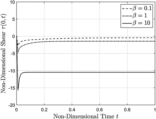
Figure 11. Velocity profiles corresponding to a sinusoidal boundary velocity, given by equations (51)₂, (54) and (55), evaluated at three different $\beta$ values at $\omega t=\pi /2$.

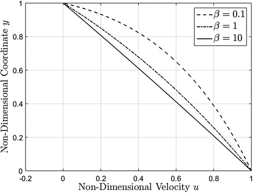
Figure 12. Velocity profiles corresponding to a sinusoidal boundary velocity, given by equations (51)₂, (54) and (55), evaluated at three different $\beta$ values at $\omega t=\pi$.

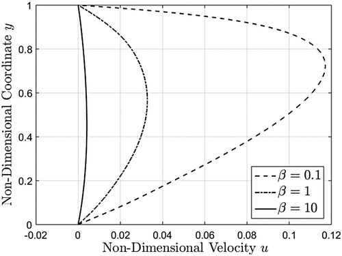
Figure 13. Velocity profiles corresponding to a sinusoidal boundary velocity, given by equations (51)₂, (54) and (55), evaluated at three different $\beta$ values at $\omega t=3\pi /2$.

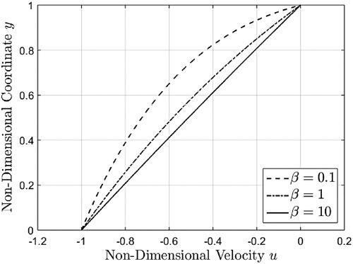
Figure 14. Midplane velocity as a function of time corresponding to a sinusoidal boundary velocity, given by equations (51)₂, (54) and (55), evaluated at three different $\beta$ values.

The shear stress profiles given by Eq. (40) are provided in Figures 7 and 8 for three values of the non-dimensional pressure $\beta$ and two different times. As it results from these figures, the shear stress in absolute value is an increase function with respect to the $\beta$ parameter and becomes constant on the whole flow domain at a small value $t=1$ of the non-dimensional time. Moreover, as indicated by Eq. (44)₂, it comes near the constant value $-1/\ln (11/10)=-10.492$ for $\beta =10$ both at time $t=0.1$ and $t=1$. Consequently, as it was to be expected, the required time to reach the steady state decreases for increasing values of pressure $\beta$.

The corresponding midplane velocity, as it results from Figure 9, also tends to a constant value and both the time it takes to reach the steady state as well as the magnitude of the steady velocity greatly varies for different values of the non-dimensional pressure $\beta$. Its steady value decreases for increasing values of $\beta$ and the steady-state is rather obtained at large values of this parameter. As regards the lower wall shear stress (see Figure 10), it tends to a local minimum in the plate vicinity before increasing to the steady state value.

Figures 11–13 depict the velocity profiles associated with the sinusoidal boundary velocity given by equations (51)₂, (54) and (55). Once again the solutions are plotted for three representative values of $\beta$ when $\omega t=\pi /2$, $\pi$ or $3\pi /2$. The boundary conditions are clearly satisfied, and the velocity oscillations can be easily observed. Note that for small values of the non-dimensional pressure $\beta$ the fluid moves faster because the viscosity is smaller.

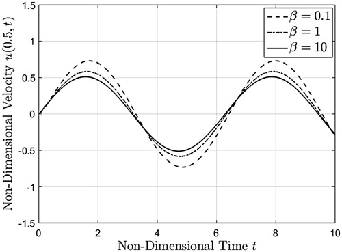
The variation of the corresponding midplane velocity is underlined in Figure 14 for the same values of $\omega t$. Here, the oscillatory specific feature of the motion is provided, and the oscillations’ amplitude decreases for increasing values of non-dimensional pressure $\beta$.

The main findings of the work presented herein are as follows:

• The motion problem of the incompressible Newtonian fluids with linear dependence of viscosity on the pressure between two infinite horizontal parallel plates, induced by the lower plate, is completely solved.

• Simple expressions for dimensionless velocity and shear stress fields are established using a suitable change of independent variable and the finite Hankel transform.

• For illustration, three special cases are considered, and two interesting results are brought to light. (1) Steady component ${\tau }_{Cp}$ of the shear stress corresponding to the simple Couette flow is constant on the whole flow domain although the adequate velocity field is a function of the spatial variable y. (2) The solutions corresponding to some motions generated by the accelerated lower plate can be obtained as simple or multiple integrations of the similar solutions for the simple Couette flow (see Eqs. (50)).

• The solutions corresponding to oscillatory motions and simple Couette flow are presented in different forms whose equivalence is graphically proved by Figures 2–4.

• The shear stress ${\tau }_C(y,t)$ in absolute value, as well as its steady component ${\tau }_{Cp}$, is an increasing function with respect to the parameter $\beta$ and tends to infinity for $\beta \to \mathrm{\infty }$.

• The asymptotic value of the midplane velocity is a decreasing function with regard to $\beta$ and steady-state is rather obtained at large values of the non-dimensional pressure.

Acknowledgements

The authors would like to express their sincere gratitude to the Editor and reviewers for their careful assessment, fruitful remarks and valuable suggestions and comments regarding the first two versions of the paper. The authors also would like to thank Prof. K.R. Rajagopal for bringing the present problem to their attention and for some fruitful and valuable suggestions.

Disclosure statement

No potential conflict of interest was reported by the author(s).

References

- Ericksen JL. Deformations possible in every isotropic, incompressible, perfectly elastic body. Z Angew Math Phys. 1954;5:466–489. doi: 10.1007/BF01601214
- Ericksen JL. Deformations possible in every compressible, isotropic, perfectly elastic material. J Math Phys. 1955;34:126–128. doi: 10.1002/sapm1955341126
- Wineman AS. Universal deformations of incompressible simple materials. University of Michigan, Technical Report, Ann Arbor, 1967.
- Carroll MM. Controllable deformations of incompressible simple materials. Int J Eng Sci. 1967;5:515–525. doi: 10.1016/0020-7225(67)90038-9
- Fosdick RL. Dynamically possible motions of incompressible, isotropic, simple materials. Arch Rat Mech Anal. 1968;29:272–288. doi: 10.1007/BF00276728
- Stokes GG. On the theories of the internal friction of fluids in motion, and of the equilibrium and motion of elastic solids. Trans Cambridge Philos Soc. 1845;8:287–305.
- Bridgman PW. The physics of high pressure. New York: The MacMillan Company; 1931.
- Cutler WG, McMickle RH, Webb W, et al. Study of the compressions of several high molecular weight hydrocarbons. J Chem Phys. 1958;29:727–740. doi: 10.1063/1.1744583
- Griest EM, Webb W, Schiessler RW. Effect of pressure on viscosity of higher hydrocarbons and their mixtures. J Chem Phys. 1958;29:711–720. doi: 10.1063/1.1744579
- Johnson KL, Cameron R. Shear behavior of elastohydrodynamic oil films at high rolling contact pressures. Proc Inst Mech Eng. 1967;182:307–330. doi: 10.1243/PIME_PROC_1967_182_029_02
- Johnson KL, Greenwood JA. Thermal analysis of an Eyring fluid in elastohydrodynamic traction. Wear. 1980;61:353–374. doi: 10.1016/0043-1648(80)90298-7
- Johnson KL, Tevaarwerk JL. Shear behavior of elastohydrodynamic oil films. Proc R Soc Lond A Math Phys Sci. 1977;356:215–236.
- Bair S, Winer WO. The high pressure high shear stress rheology of liquid lubricants. J Tribol. 1992;114:1–9. doi: 10.1115/1.2920862
- Málek J, Rajagopal KR, Růžička M. Existence and regularity of solutions and stability of the rest state for fluids with shear dependent viscosity. Math Mod Meth Appl S. 1995;05:789–812. doi: 10.1142/S0218202595000449
- Málek J, Nečas J, Rajagopal KR. Global analysis of the flows of fluids with pressure-dependent viscosities. Arch Ration Mech Anal. 2002;165:243–269. doi: 10.1007/s00205-002-0219-4
- Hron J, Málek J, Nečas J, et al. Numerical simulations and global existence of solutions of two-dimensional flows of fluids with pressure - and shear-dependent viscosities. Math Comput Simulat. 2003;61:297–315. doi: 10.1016/S0378-4754(02)00085-X
- Franta M, Málek J, Rajagopal KR. On steady flows of fluids with pressure– and shear–dependent viscosities. Proc R Soc Lend A Math Phys Sci. 2005;461:651–670. doi: 10.1098/rspa.2004.1360
- Rajagopal KR. On implicit constitutive theories. Appl Math-Czech. 2003;48:279–319. doi: 10.1023/A:1026062615145
- Rajagopal KR. On implicit constitutive theories for fluids. J Fluid Mech. 2006;550:243–249. doi: 10.1017/S0022112005008025
- Hron J, Málek J, Rajagopal KR. Simple flows of fluids with pressure–dependent viscosities. Proc R Soc Lond A Math Phys Sci. 2001;457:1603–1622. doi: 10.1098/rspa.2000.0723
- Rajagopal KR. Couette flows of fluids with pressure dependent viscosity. Int J Appl Mech Eng. 2004;9:573–585.
- Rajagopal KR. A semi-inverse problem of flows of fluids with pressure-dependent viscosities. Inverse Probl Sci En. 2008;16:269–280. doi: 10.1080/17415970701529205
- Massoudi M, Phuoc TX. Unsteady shear flow of fluids with pressure-dependent viscosity. Int J Eng Sci. 2006;44:915–926. doi: 10.1016/j.ijengsci.2006.05.010
- Srinivasan S, Rajagopal KR. Study of a variant of Stokes’ first and second problems for fluids with pressure dependent viscosities. Int J Eng Sci. 2009;47:1357–1366. doi: 10.1016/j.ijengsci.2008.11.002
- Průša V. Revisiting Stokes first and second problems for fluids with pressure-dependent viscosities. Int J Eng Sci. 2010;48:2054–2065. doi: 10.1016/j.ijengsci.2010.04.009
- Rajagopal KR, Saccomandi G, Vergori L. Unsteady flows of fluids with pressure dependent viscosity. J Math Anal Appl. 2013;404:362–372. doi: 10.1016/j.jmaa.2013.03.025
- Debnath L, Bhatta D. Integral transforms and their applications. 2nd ed Boca Raton: Chapman and Hall/CRC Press; 2007.
- Erdoğan ME. On the unsteady unidirectional flows generated by impulsive motion of a boundary or sudden application of a pressure gradient. Int J Non-Linear Mech. 2002;37:1091–1106. doi: 10.1016/S0020-7462(01)00035-X
- Rajagopal KR, Bhatnagar RK. Exact solutions for some simple flows of an Oldroyd-B fluid. Acta Mech. 1995;113:233–239. doi: 10.1007/BF01212645