
 ?Mathematical formulae have been encoded as MathML and are displayed in this HTML version using MathJax in order to improve their display. Uncheck the box to turn MathJax off. This feature requires Javascript. Click on a formula to zoom.
Abstract
In this paper we consider the identification of the initial condition for a distributed order diffusion equation. We first prove the unique existence and the regularity properties of the strong solution on the bounded temporal-spacial domain based on the eigenfunction expansions. The ill-posedness of the backward problem is interpreted by the compactness of the observation operator. Next the Laplace transformation technique and analytic continuation method are adopted to prove the uniqueness of the backward problem. Then for stabilizing the ill-posed problem, the backward problem is formulated as a Tikhonov type optimization problems, and the conjugate gradient method is adopted to solve the optimization problem with the help of the variational adjoint technique. Finally four numerical examples are given to show the efficiency and stability of the proposed method.
1. Introduction
Research during the past several decades on the anomalous diffusion equation, especially about the time fractional diffusion equation with a single-term temporal derivative, has been widely carried out by large numbers researchers due to the extensive application in describing the dynamics of physical processes involving anomalous diffusion mechanism. For example, fractional diffusion has been successfully used to modelling diffusion process in media with fractal geometry [Citation1], highly heterogeneous aquifer [Citation2] and underground water pollution problem [Citation3]. Accompanying by the numerous application of the fractional order diffusion equation, many researchers have developed different numerical methods to approximate the solution of the time-fractional diffusion equation. We refer the interested reader to [Citation4–6] for the finite element methods, [Citation7–10] for the finite difference methods, [Citation11,Citation12] for the spectral methods, etc.
In order to archive more accuracy description for some complex anomalous diffusion process with fractional order equations, many researchers detect that whose orders of the fractional derivatives may change in time and/or spatial coordinates. This yields the time-fractional diffusion equations of distributed order. The distributed order fractional derivative was firstly introduced by Caputo [Citation13], which is an integral of fractional derivatives with respect to the order on a finite interval. There are some mathematical researches to the initial-boundary value problems of the distributed order diffusion equation. The existence and the uniqueness of the solution to distributed order initial-boundary value problem was derived by the variables separation method and the maximum principle, respectively, in [Citation14]. Kochubei [Citation15] investigated the existence and the asymptotics of the solutions to the Cauchy problems for both the partial and the ordinary fractional differential equations with distributed order derivatives. Li et al. [Citation16] established the existence, uniqueness and analyticity of the solution to a distributed order time-fractional diffusion equation by adopting the Laplace transform and the eigenfunctions expansion method. In [Citation17], existence, uniqueness and regularity of the solution to the distributed order time-fractional diffusion model were given. Li et al. [Citation18] investigated some important asymptotic behaviour of solutions to initial-boundary-value problems for distributed order time fractional diffusion equations initial-boundary value problem in multi-dimensional domains.
Meanwhile, the numerical solution methods to the distributed order diffusion equation have been extensively studied, such as finite element methods [Citation19–22], reproducing kernel method [Citation23], spectral methods [Citation24], and finite difference methods, see, for example, [Citation25–30]. The idea of numerical approximation of the above mentioned numerical methods for distributed order diffusion equation is that the distributed order diffusion equation is reasonably approximated as the multi-term fractional differential equation. Essentially, the multi-term fractional differential equation is the particular case of the distributed order diffusion equation, in which the weight function is taken in form of a finite linear combination of the Dirac δ-functions with the positive weight coefficient. Henceforth, the numerical methods for the multi-term fractional differential equations are valuable to the approximation methods for the distributed order diffusion equation. Considering the numerical approximation method for the multi-term fractional diffusion equation, we refer the interested readers to [Citation31–34].
Corresponding to the research of the direct problem of the diffusion equation with the distributed order, the inverse problems of the distributed order diffusion equation are attracting considerable attention of many researchers. Li et al. [Citation35] investigated the uniqueness of determining the weight function in the distributed order time derivative by a Harnack type inequality of the solution in the frequency domain with one point observation. Applying the Stone-Weierstrass and Mntz-S
asz theorems, [Citation17] considered the uniqueness of identifying the weight function in 1-D time-fractional diffusion equation of distributed order under an important representation theorem by one point observation data or the flux at one point. Li et al. [Citation16] proved the uniqueness of recovering the weight function of distributed order time derivative by Laplace transformation with one point observation data. Zhang and Liu [Citation36] considered a time-dependent inverse source problem from a nonlocal integral observation.
In this paper, we consider the following one-dimensional distributed order initial boundary value problem
(1)
(1) with homogeneous Neumann boundary condition
(2)
(2) and initial condition
(3)
(3) where
.
is the distributed order fractional derivative defined by (Equation4
(4)
(4) ).
(4)
(4) where μ is a non-negative and continuous weighted function, and
is the left Caputo derivative of order α defined as follows
Here we consider the restructure problem of the initial function
by the measurement
at the left end point, which is the noise-contaminated data for the exact value
:
(5)
(5) where δ is some known error level. For backward problem of the time fractional diffusion equation, we refer the interested readers to references [Citation37–39].
As the initial-boundary value problem (Equation1(1)
(1) )–(Equation3
(3)
(3) ) is a linear problem, the principle of superposition holds. Without loss of generality, we assume the governing equation (Equation1
(1)
(1) ) is homogeneous, i.e.
. Next, we organize the rest of the paper as follows. In Section 2, regularizing properties of the solution to the direct problem and ill-posedness analysis to the inverse problem are presented. The uniqueness of identifying the initial condition is given in Section 3. The backward problem is transformed into a regularization optimization problem of Tikhonov-type, and the conjugate gradient algorithm is proposed to solve the regularization problem in Section 4. Finally several numerical examples are investigated in Section 5.
2. Regularity of solution for the direct problem and ill-posedness analysis for the backward problem
By , we know that the differentiation operator
is a symmetric uniformly elliptic operator. Hence the spectrum of operator
only includes the counting eigenvalues. Let
be the eigensystem of
. For convenience of derivation, we take
satisfying
and set
. From [Citation40], we see that
.
We know that the sequence forms an orthogonal basis in
. We define a fractional power
of
as follow
where the symbol
represents the inner products in
.
becomes a Hilbert space equipped with the following norm:
We have
for
.
2.1. Regularity of solution for the direct problem
Before establishing the regularity estimation of the solution to the direct problem, we first define a strong solution to problem (Equation1(1)
(1) )–(Equation3
(3)
(3) ) as follows.
Definition 2.1
We say that u is a strong solution to the initial-boundary value problem (Equation1(1)
(1) )–(Equation3
(3)
(3) ) with f = 0 if (1) hold in
and
for almost all
, and
, and (Equation2
(2)
(2) ) holds for all
,
.
In order to prove the existence of a unique strong solution to the direct problem (Equation1(1)
(1) )–(Equation3
(3)
(3) ), we first consider the properties of the following ordinary distributed fractional order differentiation equation.
(6)
(6) Applying Laplace transform to (Equation6
(6)
(6) ), we get
where
is the phase function of the Laplace transformation for v. Solving the above algebraic equation, we have
where auxiliary function
is defined as follows
By cutting along the negative part of the real axis, we can extend the function
to an analytic function by taking the principal value of the logarithmic function on the complex plane with the cut. Meanwhile, it is easy to know that the function
has no singularities on the main sheet of the Riemann surface for the logarithmic function. As matter of fact, for
, the imaginary part of
, i.e.
is equal to zero only if
. If
and
, we have
. Therefore,
is an analytic function on the main sheet of the Riemann surface of the complex plane cut along the negative part of the real axis. Next, we go to analyse the regularity of the solution to problem (Equation1
(1)
(1) )–(Equation3
(3)
(3) ). Based on the idea of reference [Citation18], we firstly define a useful contour
including three parts on the complex plane as follows
arg
,
arg
where For the completeness, we introduce the Lemmas 2.1 and 2.2 which are proved in reference [Citation15] and in reference [Citation18], respectively.
Lemma 2.1
[Citation15]
If and
the solution
to (Equation6
(6)
(6) ) is continuous at the origin t, completely monotone and belongs to
.
Lemma 2.2
[Citation18]
If is a non-negative function satisfying
we have
and
where
and C>0 is a constant independent of λ and s.
With the help of the above lemma, we go to estimate the solution to problem (Equation6(6)
(6) ).
Theorem 2.1
If and
there exists a unique solution
to (Equation6
(6)
(6) ), satisfying
.
Proof.
By Fourier–Mellin formula (see e.g. [Citation41]), we obtain
Applying the residue theorem, for t>0 we know that the inverse Laplace transform of
can be reformulated as the following integral along the contour
If
, by the additivity of integration, we have
(7)
(7) Writing the complex variable s as
, by Lemma 2.2 and
, we have
(8)
(8)
Similarly, by the additivity of integration, we have
If
, we have
. By direct derivation, we get
Let
be a sufficiently small positive constant. We set
,
. Therefore, we have
Obviously, we have
if
and
if
and
, which yields the following inequalities
Collecting the above two inequalities, we obtain
(9)
(9) Next, we consider the last integral
.
(10)
(10)
As μ is a non-negative and continuous weighted function on
and meets
, there exists a constant
such that
. Then for any
, we have
For
, we have
By (Equation10
(10)
(10) ), we have
(11)
(11)
From (Equation8
(8)
(8) ), (Equation9
(9)
(9) ) and (Equation11
(11)
(11) ), we have
Next, we consider the case of
. Obviously, there exists a constant
and
that meets the condition
for any
such that
. Similarly, by the additivity of integration, we have
(12)
(12) By Lemma 2.2, we get
(13)
(13)
Obviously, we have
Let
, by direct estimation, we have
So, we obtain
(14)
(14) Since
, we have
(15)
(15)
By
and (Equation13
(13)
(13) ), (Equation14
(14)
(14) ) and (Equation15
(15)
(15) ), we have
(16)
(16) This finishes the proof of theorem.
Theorem 2.2
If then there exists a unique strong solution to (Equation1
(1)
(1) )–(Equation3
(3)
(3) ) and the solution
can be represented as follows
(17)
(17) where
is the Fourier coefficient of
, i.e.
and
Moreover, we have the following estimates
Proof.
Applying the separation of variables, we can derive a solution of series form to the direct problem (Equation1(1)
(1) )–(Equation3
(3)
(3) ) as (Equation17
(17)
(17) )(see (3.1) in [Citation18]). We will verify that (Equation17
(17)
(17) ) certainly means a strong solution to (Equation1
(1)
(1) )–(Equation3
(3)
(3) ). From the Lemma 2.1, we know that
is completely monotone. So we have
and
We first have
Moreover by Theorem 2.1, i.e.
If we take
, we have
Similarly, by Theorem 2.1, we obtain
and
Hence, we get
Obviously, we have
The uniqueness of strong solution lies in the uniqueness of the ordinary fractional differential equation (Equation6
(6)
(6) )(see Lemma 2.2 in [Citation17], for example). The proof of the theorem is completed.
2.2. Ill-posedness analysis for the backward problem
We defining a linear operator
as follows:
(18)
(18)
Theorem 2.3
The observation operator is compact.
Proof.
We will prove the compactness of the observation operator . Defining the finite dimensional operators
as follows:
(19)
(19) Set
, from (Equation18
(18)
(18) ), (Equation19
(19)
(19) ) and Theorem 2.1, we obtain
By
, obviously,
in the sense of operator norm in
as
. Therefore,
is a compact operator.
From the Theorem 2.3, we know that identifying initial condition in
from the observation data
in
is ill-posed. Some regularization strategies should be considered. We will adopt the Tikhonov regularization method to deal with the backward problem in Section 4.
3. Uniqueness
In order to explore the unique theorem of the backward problem, first we need to prove the following lemma.
Lemma 3.1
Assume
there exist a unique strong solution
to direct problem (Equation1
(1)
(1) )–(Equation3
(3)
(3) ). Moreover, we have the following estimate
if
,
Proof.
From the Theorem 2.2, the unique strong solution is given by (Equation17(17)
(17) ). We have
As
, we obtain
. By the Sobolev embedding theorem, we get
Note that
. If
, take ε satisfying
from Theorem 2.1 we have
From the above inequality, we have
The proof of the lemma is finished.
Theorem 3.1
Assume the initial function
can be identified uniquely by the observation data at left end point, i.e.
.
Proof.
From Lemma 3.1, the observation data is meaningful if
. By contradiction, we assume there exist two different functions, denoting by
i = 1, 2. The solutions about
and
, respectively, are expressed as follows
where
,
By Lemma 3.1, the two series
and
are uniformly convergent on interval
. Applying analytic continuation technique, we know that the above two series are uniform convergence on
. By Lemma 3.1, one have
As
is integral in
for fixed z such that
. Taking Laplace transform with respect to the time variable t on the both sides of equation
, by the Lebesgue dominated convergence theorem, we have
(20)
(20) Therefore, (Equation20
(20)
(20) ) yields
That is
(21)
(21) We know that
is internally closed uniform convergence in
. So, applying the Weierstrass theorem, we can analytically continue
in η and (Equation21
(21)
(21) ) holds for
. We take a small disk which only includes
and does not include others. Integrating (Equation21
(21)
(21) ) in the disk, we get
, which means
as
. Repeating this procedure, we have
Therefore, we obtain
The proof of the theorem is completed.
4. Variational optimization and the conjugate gradient method
From the above ill-posedness analysis, we know the backward problem is ill-posed. In order to obtain the stable numerical solution of the backward problem, we adopt the classic Tikhonov regularization method to deal with this problem. Define a Tikhonov regularization functional as follows
(22)
(22) where β is a regularization parameter. Therefore, the backward problem is transformed into the following variational optimization problem
From the theory of the classic Tikhonov regularization, we see that the minimizer
exists uniquely and converges to the exact initial function
if a suitable regularization parameter β is chosen, see Theorems 5.1–5.2 in [Citation42]. In this paper, we adopt the conjugate gradient method (CGM) to seek the minimizer of functional (Equation22
(22)
(22) ). As we know, the key step of using the conjugate gradient method is to find the gradient of the functional (Equation22
(22)
(22) ). Here we compute the functional gradient by the means of the variational adjoint technique.
In the following, we derive formally the gradient of the regularization functional with the help of variational adjoint method. Let be a small perturbation of initial function
, then the small change
of the solution to the forward problem (Equation1
(1)
(1) )–(Equation3
(3)
(3) ) satisfies
(23)
(23)
For obtaining the gradient of the optimization functional (Equation22
(22)
(22) ), we firstly calculate the first order variation of functional (Equation22
(22)
(22) ). From (Equation22
(22)
(22) ), we have
(24)
(24)
Let
be a smooth function, multiplying both side of governing equation in (Equation23
(23)
(23) ) by
and integrating with respect to the temporal-spatial variables on
, we have
After interchanging the integral variables of t and τ two times and integrating by parts, we have
(25)
(25)
Combing (Equation24
(24)
(24) ) with (Equation25
(25)
(25) ), we define the adjoint problem as follows
(26)
(26)
where
is the Caputo fractional right derivative defined by
From the equality (Equation25
(25)
(25) ) and adjoint problem (Equation26
(26)
(26) ), we have
(27)
(27) By (Equation24
(24)
(24) ) and (Equation27
(27)
(27) ), we obtain
(28)
(28) Assume that
is the k-th approximate solution of
. Set
(29)
(29) where
is a descent direction and
is the step size in the k-th iteration. The descent direction of the CGM is updated by using the following iteration formula
(30)
(30) where
is conjugate coefficient updated by
(31)
(31) The optimal descent step size
in the k-th iteration can be obtained by minimizing the problem (Equation32
(32)
(32) ). From (Equation22
(22)
(22) ), we have
(32)
(32) Take
we obtain the k-th iteration optimal step size as follows
(33)
(33) For the fixed regularization parameter β, we take the CGM to solve the optimization problem (Equation22
(22)
(22) ) by adopting the well-known Morozovs discrepancy principle as the stopping condition, i.e. we choose
satisfying the following inequality:
(34)
(34) where
is a positive constant,
. So, we obtain the CGM to solve the optimization problem with the fixed regularization parameter β as follows
In the numerical implementations, we apply quasi-optimality criterion [Citation43] to choose β, i.e. we give a decreasing regularization parameter sequence of ,
is a positive constant, and choose
as the minimizer of
. Therefore, we formulate the inversion algorithm based on the CGM as follows
5. Numerical examples
In this section, we present several numerical examples to illustrate the effectiveness of the conjugate gradient algorithm. Without loss of generality, we take ,
and T = 1 for all the numerical simulations. To obtain the (noisy) observation data
, we first give the true initial function
and solve the direct problem (Equation1
(1)
(1) )–(Equation3
(3)
(3) ) by finite difference method proposed in [Citation29], then add pointwise noise by
, where
is the discretization time nodal point, δ is the noise level and ξ is a uniform random variable in
.
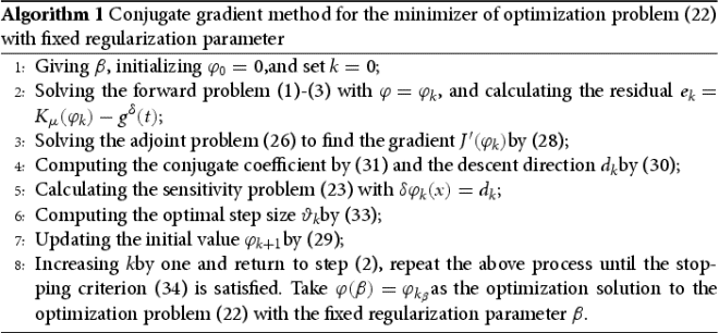
Example 5.1
Let ,
,
,
. We take
as the exact initial condition, and the direct problem (Equation1
(1)
(1) )–(Equation3
(3)
(3) ) has exact solution
.
Example 5.2
Let ,
,
,
. We take
as the exact initial function, and the direct problem (Equation1
(1)
(1) )–(Equation3
(3)
(3) ) has no exact solution.
Numerical results for Examples 5.1 and 5.2 are showed in Figures , and Table with relative noise level ,
,
and
, respectively. From the Table , we see the inversion solution becomes much closer to the exact solution when the relative error level becomes much smaller.
Figure 1. inversion solution for Example 5.1.
Figure 2. inversion solution for Example 5.2.
Table 1. Inversion results for the four numerical examples with different relative errors.
Example 5.3
Let ,
,
,
. We take
as the exact initial condition. The exact solution to the direct problem (Equation1
(1)
(1) )–(Equation3
(3)
(3) ) can be given explicitly as
.
Example 5.4
Let ,
,
,
. The exact initial function is taken as
, and the exact solution to the direct problem (Equation1
(1)
(1) )–(Equation3
(3)
(3) ) is unknown.
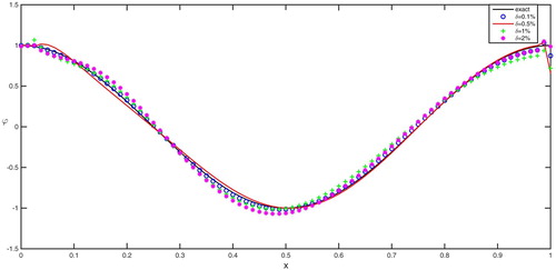
The reconstructions for Examples 5.3 and 5.4 are exhibited in Figures , and Table . The relative noise levels for Examples 5.3, 5.4 are also chosen as , respectively. From Table , we find the inversion results become worse as noise level δ becomes larger, which shows the inversion algorithm is stable. The CPU time for above every numerical inversion problems is around 110 seconds with the computer configuration as follows, System: Microsoft Windows; CPU: inter(R) core(TM) i7-4500U @ 2.40 GHz; RAM:8.00 GB.
Figure 3. inversion solution for Example 5.3.
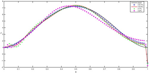
Figure 4. inversion solution for Example 5.4.
6. Conclusions
In this paper, we consider the identification problem of initial function for one-dimensional distributed order diffusion equation. The unique existence and the regularity properties of the strong solution are established by the eigenfunction expansions. Based on the uniform convergence of the observation operator, we interpret the ill-posedness of the backward problem. The uniqueness of the backward problem is proven by Laplace transformation technique and analytic continuation method. Several numerical examples show that the inversion algorithm based on the conjugate gradient method is effective and stable.
Disclosure statement
No potential conflict of interest was reported by the author(s).
Additional information
Funding
References
- Nigmatullin RR. The realization of the generalized transfer equation in a medium with fractal geometry. Phys Status Solidi (b). 1986;133(1):425–430.
- Adams EE, Gelhar LW. Field study of dispersion in a heterogeneous aquifer: 2. spatial moments analysis. Water Resour Res. 1992;28(12):3293–3307.
- Hatano Y, Hatano N. Dispersive transport of ions in column experiments: an explanation of long-tailed profiles. Water Resour Res. 1998;34(5):1027–1033.
- Jiang Y, Ma J. High-order finite element methods for time-fractional partial differential equations. J Comput Appl Math. 2011;235(11):3285–3290.
- Ford NJ, Xiao J, Yan Y. A finite element method for time fractional partial differential equations. Fract Calc Appl Anal. 2011;14(3):454–474.
- Zeng F, Li C, Liu F, et al. The use of finite difference/element approaches for solving the time-fractional subdiffusion equation. SIAM J Sci Comput. 2013;35(6):A2976–A3000.
- Yuste SB. Weighted average finite difference methods for fractional diffusion equations. J Comput Phys. 2006;216(1):264–274.
- Murio DA. Implicit finite difference approximation for time fractional diffusion equations. Comput Math Appl. 2008;56(4):1138–1145.
- Cui M. Compact finite difference method for the fractional diffusion equation. J Comput Phys. 2009;228(20):7792–7804.
- Gao G, Sun Z. A compact finite difference scheme for the fractional sub-diffusion equations. J Comput Phys. 2011;230(3):586–595.
- Lin Y, Xu C. Finite difference/spectral approximations for the time-fractional diffusion equation. J Comput Phys. 2007;225(2):1533–1552.
- Li X, Xu C. A space-time spectral method for the time fractional diffusion equation. SIAM J Numer Anal. 2009;47(3):2108–2131.
- Caputo M. Mean fractional-order-derivatives differential equations and filters. Annali DellUniversita Di Ferrara. 1995;41(1):73–84.
- Luchko Y. Boundary value problems for the generalized time-fractional diffusion equation of distributed order. Fract Calc Appl Anal. 2009;12(4):409–422.
- Kochubei AN. Distributed order calculus and equations of ultraslow diffusion. J Math Anal Appl. 2008;340:252–281.
- Li Z, Luchko Y, Yamamoto M. Analyticity of solutions to a distributed order time-fractional diffusion equation and its application to an inverse problem. Comput Math Appl. 2017;73(6):1041–1052.
- Rundell W, Zhang Z. Fractional diffusion: recovering the distributed fractional derivative from overposed data. Inverse Problems. 2017;33(3):035008.
- Li Z, Luchko Y, Yamamoto M. Asymptotic estimates of solutions to initial-boundary-value problems for distributed order time-fractional diffusion equations. Fract Calc Appl Anal. 2014;17(4):1114–1136.
- Jin B, Lazarov R, Sheen D, et al. Error estimates for approximations of distributed order time fractional diffusion with nonsmooth data. Fract Calc Appl Anal. 2016;19(1):69–93.
- Bu W, Xiao A, Zeng W. Finite difference/finite element methods for distributed-order time fractional diffusion equations. J Sci Comput. 2017;72(1):422–441.
- Wei L, Liu L, Sun H. Stability and convergence of a local discontinuous Galerkin method for the fractional diffusion equation with distributed order. J Appl Math Comput. 2019;59(1–2):323–341.
- Abbaszadeh M, Dehghan M. Numerical and analytical investigations for neutral delay fractional damped diffusion-wave equation based on the stabilized interpolating element free Galerkin (IEFG) method. Appl Numer Math. 2019;145:488–506.
- Li XY, Wu BY. A numerical method for solving distributed order diffusion equations. Appl Math Lett. 2016;53:92–99.
- Chen H, L S, Chen W. Finite difference/spectral approximations for the distributed order time fractional reaction–diffusion equation on an unbounded domain. J Comput Phys. 2016;315:84–97.
- Hu X, Liu F, Anh V, et al. A numerical investigation of the time distributed-order diffusion model. ANZIAM J. 2014;55:464–478.
- Ye H, Liu F, Anh V. Compact difference scheme for distributed-order time-fractional diffusion-wave equation on bounded domains. J Comput Phys. 2015;298:652–660.
- Morgado ML, Rebelo M. Numerical approximation of distributed order reaction–diffusion equations. J Comput Appl Math. 2015;275:216–227.
- Gao GH, Sun ZZ. Two alternating direction implicit difference schemes for two-dimensional distributed-order fractional diffusion equations. J Sci Comput. 2016;66(3):1281–1312.
- Li X, Rui H. A block-centered finite difference method for the distributed-order time-fractional diffusion-wave equation. Appl Numer Math. 2018;131:123–139.
- Abbaszadeh M, Dehghan M. Meshless upwind local radial basis function-finite difference technique to simulate the time- fractional distributed-order advection-diffusion equation. Eng Comput. 2019. doi: 10.1007/s00366-019-00861-7
- Jin B, Lazarov R, Liu Y, et al. The Galerkin finite element method for a multi-term time-fractional diffusion equation. J Comput Phys. 2015;281:825–843.
- Zheng M, Liu F, Anh V, et al. A high-order spectral method for the multi-term time-fractional diffusion equations. Appl Math Model. 2016;40(7–8):4970–4985.
- Zhao Y, Zhang Y, Liu F, et al. Convergence and superconvergence of a fully-discrete scheme for multi-term time fractional diffusion equations. Comput Math Appl. 2017;73(6):1087–1099.
- Gao G, Alikhanov AA, Sun Z. The temporal second order difference schemes based on the interpolation approximation for solving the time multi-term and distributed-order fractional sub-diffusion equations. J Sci Comput. 2017;73(1):93–121.
- Li ZY, Fujishiro K, Li GS. An inverse problem for distributed order time-fractional diffusion equations. [cited 2018 Aug 10]. Available from: http://arxiv.org/abs/1707.02556v2
- Zhang M, Liu J. Identification of a time-dependent source term in a distributed-order time-fractional equation from a nonlocal integral observation. Comput Math Appl. 2019;78(10):3375–3389.
- Liu JJ, Yamamoto M. A backward problem for the time-fractional diffusion equation. Appl Anal. 2010;89(11):1769–1788.
- Wang L, Liu J. Data regularization for a backward time-fractional diffusion problem. Comput Math Appl. 2012;64(11):3613–3626.
- Wang JG, Wei T, Zhou YB. Tikhonov regularization method for a backward problem for the time-fractional diffusion equation. Appl Math Model. 2013;37(18–19):8518–8532.
- Levitan BM, Sargsian IS. Introduction to spectral theory: selfadjoint ordinary differential operators. Providence (RI): American Mathematical Society; 1975.
- Schiff JL. The Laplace transform: theory and applications. New York (NY): Springer Science & Business Media; 2013.
- Engl HW, Hanke M, Neubauer A. Regularization of inverse problems. Dordrecht: Kluwer Academic Publisher; 1996.
- Tikhonov AN, Glasko V. Use of the regularization method in non-linear problems. USSR Comput Math Math Phys. 1965;5(3):93–107.