Current distribution reconstruction in switching arcs by means of regularization based on GSVD

Abstract

The knowledge of the variation of arc current is helpful in improving the breaking performance of a vacuum circuit breaker. As a novel non-intrusive method, arc magnetic performance testing technology has attracted attention. In view of the widely used regularization method of the standard form in arc current reconstructions cannot fully overcome the ill-posed nature of the Biot-Savart equation, the regularization approach based on generalized singular value decomposition (GSVD) is proposed to improve the situation. Moreover, a discrete 3-D arc model with the help of the finite element technique incorporating the current divergence-free and boundary conditions is introduced to improve the authenticity of the model. The performance of the truncated generalized singular value decomposition (TGSVD) and general-form Tikhonov regularization with derivative operators L₁ and L₂ are studied in numerical tests. In addition, the effectiveness of generalized cross validation criterion, quasi optimality criterion and normalized cumulative periodic graph method in selecting regularization parameters are compared. The methodology can help improve arc control and guide the design of vacuum circuit breakers with improved performance parameters.

KEYWORDS:

• Electromagnetic inverse problems
• arc inversion
• finite element technique
• GSVD
• regularization parameter selection

2010 MATHEMATICS SUBJECT CLASSIFICATIONS:

• 65J22
• 65F22
• 65M60
• 35Q61

1. Introduction

In switchgear with contacts, vacuum circuit breakers (VCBs) inevitably ignite arcs during the switching process. The current density distribution of the arc is one of the factors that determine the spatial variation of the heat flux, the temperature of the metal vapour vacuum arc, and the rate of electrode erosion in the vacuum interrupter. At present, investigative approaches to the switching arc consist of combinations of experimental and numerical analysis. Experimental approaches make use of charge- coupled device (CCD) cameras, optical fibre arrays, spectrum analysis, and magnetic diagnostics. The first three methods use optical testing and require drilling holes in the interrupter walls or the use of transparent wall materials to observe the dynamic arc characteristics. These optical methods are intrusive as the modifications affect the physical properties and pressure distribution in the interrupter.

Being non-intrusive, magnetic diagnostics are a promising approach. Several researchers have pursued this approach. Some have captured the arc position and arc shape by assuming the arc column and conductors in the interrupter to be a succession of 2-D rectilinear, threadlike current segments, but without any investigation of the current density [1–4]. Zhang et al. proposed the simulated annealing (SA) algorithm to reconstruct the arc shape and current distribution at various points during switching [5]. Zhao et al. verified that the genetic algorithm (GA) combined with the regularization method can effectively improve the accuracy of two-dimensional arc current reconstruction [6]. Ghezzi et al. investigated a vacuum circuit breaker model with butt electrodes and proposed ordinary Tikhonov and truncated singular value decomposition (TSVD) regularization to obtain the current density and macroscopic shape of the arc [7]. Dong et al. proposed a 2-D low-voltage circuit breaker (LVCB) model with a discussion of the performance of the regularization parameter selection strategies in reconstructing the current distribution [8]. Based on the 2-D LVCB model, the influence of magnetic measurement modelling on the solutions has been analyzed by taking random variations in the sensor positions and orientations into account [9], and the effect of magnetization in splitters on the inverse solutions have been considered by taking the magnetization as a mapping from the source domain [10].

The key to arc inversion problems is how to address the ill-posed nature of the electromagnetic forward operator. Related studies have been carried out in fields such as magnetic tomography in fuel cells. Kress et al. treated the fuel cell geometry as a cuboid and reconstructed the current distributions based on the magnetic field outside the current flow area [11]. Hauer et al. studied the characterization of the null space N(W) and orthogonal space N(W)^⊥ of the Biot-Savart operator [12]. This characterization is crucial for the evaluation of the limitations of magnetic tomography for fuel cells. The divergence-free and boundary value conditions have been treated as prior knowledge and incorporated into the Tikhonov regularization to improve the current reconstruction efficiency [13]. Additional fuel cell research expanded the fuel cell grid model using a finite integration technique to find the numerical solution of the continuous problem, proving the solvability of the grid model and convergence of the solution to the continuous problem [14]. A new magnetic tomography approach that uses current basis functions and a sensor array configuration developed to be sensitive only to current inhomogeneity has also been presented [15].

In other applications of electromagnetic inverse problems, Ghasemifard et al. developed a method for determining the currents in a set of parallel, infinitely long conductors from measured magnetic fields [16]. Jeon et al. proposed an improved harmonic algorithm for magnetic resonance electrical impedance tomography to reduce the number of iterations [17]. Marion et al. performed sensitivity analysis for the reconstruction of small-amplitude perturbations in the electric properties from boundary measurements of electric field [18]. For the inverse problem of load identification, Liu et al. proposed the identification of the dynamic load for uncertain structures based on the shape function method and interval analysis [19]. A novel interpolation-based method is proposed instead of a conventional Green kernel function method to achieve a well-posed global kernel function matrix and identify a load accurately without any regularization [20]. Sun et al. proposed a novel regularization operator to identify dynamic loads and proved its stability and effectiveness through numerical simulations [21].

Based on the GSVD, Hansen analyzed the Tikhonov regularization in a general form and defined the TGSVD solution, and generalized solution transformed to standard form is introduced [22]. In this work, the derivative operators L₁ and L₂ are adopted as alternatives to the standard form. The methods are proved to be able to invert the arc current distribution with satisfactory results. Moreover, the performances of three regularization parameter selection strategies: GCV, QO and NCP with different regularization schemes are studied. Since only standard form regularizations are employed in arc current reconstructions, it is necessary to expand the existing regularization methods.

In this paper, the arc model and the electromagnetic forward analysis are formulated and the methodology and theory are presented. Moreover, numerical results and discussions are illustrated.

2. Discrete arc model and corresponding hypothesis

The work focuses on a 40.5kV/31.5kA VCB with axial magnetic field (AMF) contacts. In the breaking process for the VCB, an arc will be generated. When the contacts moving along the Z-axis at a given speed, the arc column elongates and diffuses gradually. Figure 1 shows a 3-D structure of the VI with contact radius of R = 29 mm. The gap of distance h = 6 mm is concerned.

Figure 1. The structure of the AMF vacuum interrupter (VI) and the magnetic sampling points.

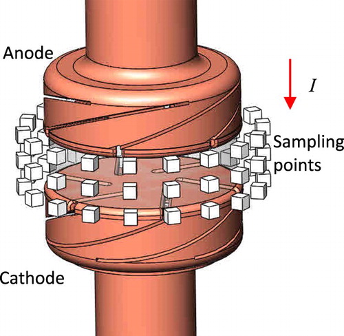
The magnetic sampling points are 30 mm away from the arc column axis. These points are distributed uniformly on a cylindrical surface coaxial with and symmetrically centered onto the arc column, as shown in Figure 1. Each point array plane is 3mm apart and each array contains 18 points, resulting in the total number of the points M = 54.

In the forward analysis, the assumptions are as follows:

1. The radius of the arc roots are supposed to be known on the cathode and anode plates in the numerical simulation.

2. The interference of the contacts and the conducting rod on the magnetic simulation of the arc is not considered.

3. The time variants in Maxwell equations are ignored, thus the problem is restricted to the quasi-static situation.

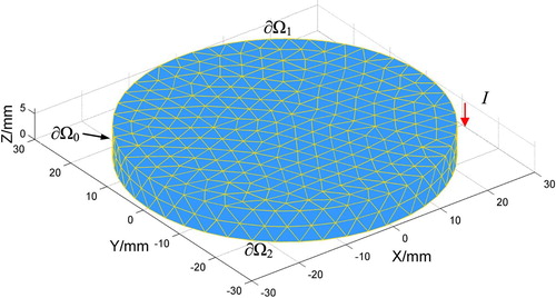
The gap which holds both the arc column and the medium is discretized into tetrahedral meshes, which is shown in Figure 2. We denote t, f, e, and n as the sets of the tetrahedrons, faces, edges and nodes, respectively. The number of the sets is denoted as |t|, |f|, |e| and |n|. A finer network can approximate the real physical model, but too many discrete elements mean a larger scale property of the problem. The dimension of this model is |t| = 2666, |f| = 5863, |e| = 3928, |n| = 732.

Figure 2. Discrete mesh of the current flow region.

From the stationary Maxwell equations, the current density is governed by the divergence-free condition, i.e. (1) $\mathrm{\nabla }\cdot j=0$(1)

Let G denotes the incidence matrix mapping from the edge set e to node set n, i.e. $G\in R^{|n|\times |e|}$. The element G_ij = +1 if the j^th edge starts from the i^th node; or G_ij = −1, if the j^th edge ends at the i^th node; otherwise G_ij = 0. The divergence-free condition (2) is complemented by the boundary condition, which is given by (2) ${\int }_{\mathrm{\partial }{\mathrm{\Omega }}_i}j\cdot dS=I_i,(i=0,1,2)$(2) where j is the edge current and I₁ = I_tot is the total current flowing through the boundary ∂Ω₁. The total current I_tot = 31.5 kA is concerned. And no current flow through the side walls ∂Ω₀ of the region Ω, i.e. I₀ = 0. Concerning the boundary condition (2), the discrete form of Equation (1) is given by Equation (3): (3) $Gj=g$(3) where $g\in R^{|n|}$ is the vector collecting the nodal current unbalances. The element g_i is calculated as $g_i=I_{tot}/n_{anode}$ for the i^th node within the radius of the anode root, and $g_j=-I_{tot}/n_{cathode}$ for the j^th node within the radius of the cathode root, where n_anode and n_cathode is the number of the anode spots and the cathode spots, respectively. The Equation (3) is underdetermined. Therefore, we need to consider the electric field condition (4) as a supplement to Equation (3): (4) $\mathrm{\nabla }\times E=0,j=\sigma E$(4) where σ is the conductivity and E is the electric field. Define incidence matrix $D\in R^{|f|\times |e|}$ mapping from the face set f to the edge set e, such that the element D_ij = +Re or − Re, respectively, if edge e_j belongs to the face f_i with the same or opposite orientation; otherwise D_ij = 0, where Re denotes the resistance of the edge. To be simplified, a uniform resistance distribution is assumed in the gap. The discrete form of Equation (4) is given by Equation (5): (5) $Dj=0$(5)

The two Equations (3) and (5) are merged to form Equation (6): (6) $\left(\begin{array}{c}G\\ D\end{array}\right)j=\left(\begin{array}{c}g\\ 0\end{array}\right)$(6)

From $|f|+|n|>|e|$, Equation (6) is sufficient to know the edge current distribution. The solution of (6) is known to be the Ohmic current and denoted as j₀. Let N denotes the nullspace of G. Thus for arbitrary vector$x\in R^{|N|}$, x satisfies $GNx=0$. The synthesized current distribution $j_{ref}$ can be written as follows and satisfies the constraints (1)–(2). (7) $j_{ref}=j_0+Nx$(7)

The magnetic field at sampling point r = (x, y, z) produced by the edge current j can be calculated according to Biot-Savart’s law: (8) $Wj(r_s)=\frac{{\mu }_0}{4\pi }{\int }_l\frac{j(r_s)\times (r-r_s)}{{|r-r_s|}^3}dl$(8) where r and r_s is the coordinate of the field and source vector, respectively. Therefore, the Biot-Savart operator in matrix form is given by Equation (9): (9) $W{j}_{ref}=b_{ref}$(9) where W_ij represents the i^th magnetic contribution corresponding to the j^th edge current. The Equations (7) and (9) are merged to form Equation (10): (10) $WNx=b_{ref}-W{j}_0$(10)

From the above discussion, the problem is reduced to solve the unknown vector $x\in R^{|N|}$ instead of inverting edge current distribution $j_{ref}$ directly from the magnetic $b_{ref}$. The linear least-squares problem is expressed as: (11) $\underset{x}{min}||WNx-(b_{ref}-W{j}_0)||$(11) Define $A=WN$, $b=b_{ref}-W{j}_0$, then Equation (11) is clearly written as (12) $\underset{x}{min}||Ax-b||$(12)

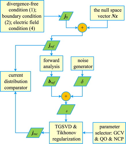
In the numerical test, Gaussian white noise δ is superimposed on the pure magnetic data and defined as follows, (13) $\delta =r\cdot std(b_{ref})\cdot randn$(13) yielding the artificial magnetic data $b_{\delta }=b_{ref}+\delta$, where r denotes the noise-to-signal ratio and $std(\cdot )$ denotes the standard deviation. The generator $randn$ produces the same standard normal distribution sequence in every inversion process. The noise is imposed on the magnetic field components b_x, b_y, b_z respectively as shown in Figure 3. The Gaussian white noise is an independent random sequence, and thus, it adequately represents real-world perturbations. The noise level r = 10⁻² is concerned. The overall flowchart of the simulation to study the performance of the method is shown in Figure 4.

Figure 3. The calculated x,y,z-component magnetic field data with the noise r = 10⁻² via forward analysis.

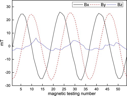
Figure 4. Flowchart of the GSVD regularization.

3. General-form regularization

3.1. The desirability of using GSVD

To study whether the regularization in general form can guarantee the calculation of satisfactory solution, we use truncated SVD and truncated GSVD to compute the solution of Equation (12). The exact solution is a linear sequence distributed in the interval [0, 2], together with the first 4 TSVD and TGSVD solutions are shown in Figure 5. The results presented in Figure 5(a) show that the solutions of TSVD contain violent fluctuations and none of these solutions can approximate close enough to the exact solution. The phenomenon still occurs even for the optimal regularization parameter of TSVD. On the other hand, Figure 5(b) shows that the first four solutions of TGSVD with L = L₁ are quite smooth and in good agreement with the exact solution. The result in Figure 5(c) shows that the results of L₂ are very good with the first 3 truncated parameters. However the fourth solution begins to fluctuate and diverge from the exact solution.

Figure 5. Comparison of TSVD and TGSVD solutions for problem (12), the abscissa represents the dimension of the solution. The noise level r = 10⁻² is applied: (a) the first 4 TSVD solutions; (b) the first 4 TGSVD solutions when L = L₁; (c) the first 4 TGSVD solutions when L = L₂.

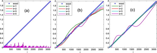
Hansen validated that the SVD vectors v_i has undesired irregular localized oscillations that did not appear in the GSVD vectors x_i [23], which is consistent with the calculation results in Figure 5. The tests show that regularization based on GSVD is able to ensure the acquisition of satisfactory solution.

3.2. The SVD/GSVD

The singular value decomposition (SVD) is one of the common methods for solving ill-posed equations such as (12). For the underdetermined problem, the SVD of $A\in R^{m\times n}$(m < n), is expressed as: (14) $A=U\mathrm{\Sigma }{V}^T=\sum _{i=1}^m{\sigma }_i{u}_i{v}_i^T$(14) where U = (u₁, u₂, … , u_m) ∈ R^m×m and V = (v₁, v₂, … , v_m) ∈ R^n×m are matrices with orthonormal columns, i.e. $U^{T}U=V^{T}V=I_m$ and Σ is a diagonal matrix with nonnegative elements arranged in non-increasing order σ₁ ≥ σ₂ ≥ … ≥ σ_m.

The GSVD method is the general-form of the SVD. The generalized singular values of the matrix pair (A, L) are the square roots of the matrix pair $(A^{T}A,L^{T}L)$. The matrix L must have the same column number as A, and if $L\in R^{p\times n}$, the dimensions must satisfy the relation $m+p>n$. The GSVD of underdetermined systems is to some extent more complicated than the overdetermined ones and given by Equation (15): (15) $A=U\left(O_{m\times (n-m)}\begin{array}{cc}\mathrm{\Sigma }& O\\ O& I_{n-p}\end{array}\right)X^{-1},L=V\left(\begin{array}{cc}{I}_{n-m}& O\\ O& M\end{array}{O}_{p\times (n-p)}\right)X^{-1}$(15) where $U\in R^{m\times m}$, $U^{T}U=I_m$, $V\in R^{p\times p}$, and $V^{T}V=I_p$ are orthonormal column matrices, and $X\in R^{n\times n}$ is nonsingular. The matrices $\sum =diag({\sigma }_i)$ and $M=diag({\mu }_i)$ are $p-(n-m)$ order diagonal matrices whose diagonal elements satisfy ${\sigma }_i^2+{\mu }_i^2=1$ and are ordered as: (16) $\{\begin{array}{l}0\le {\sigma }_1\le \dots \le {\sigma }_{p-(n-m)}\le 1\\ 1\ge {\mu }_1\ge \dots \ge {\mu }_{p-(n-m)}\ge 0\end{array}$(16)

Each generalized singular value of the matrix pair (A, L) is given by Equation (17): (17) ${\gamma }_i=\frac{{\sigma }_i}{{\mu }_i},i=1,\dots ,p-(n-m)$(17)

The columns of matrix X form the regularized solution of the GSVD. Hansen proved that X is bounded as follows [24]:

Theorem 3.1:

If $Z=\left(\begin{array}{c}A\\ L\end{array}\right)$, $P_{N(L)}$ denotes the projection matrix onto the null space N(L), and $inf(A{P}_{N(L)})$ denotes the smallest nonzero singular value of $A{P}_{N(L)}$, then (18) $||X^{-1}||=||Z||\le ||A||+||L||,||X||=\Vert Z^{+}\Vert \le {\mathrm{\Pi }}_p^{-1}$(18) where $\prod _p$ is defined by (19) ${\mathrm{\Pi }}_p\equiv \{\begin{array}{l}min\{{||L^{+}||}^{-1},inf(A{P}_{N(L)})\},p<n\\ {||L^{+}||}^{-1},p=n\end{array}$(19) From Theorem 1, we know that L should be well conditioned because $||X||$ is approximately bounded by $||L^{+}||$.

3.3. TGSVD method and general-form Tikhonov regularization

The TSVD method replaces A by a matrix A_k that is close to A and is mathematically rank deficient, where k denotes the truncation parameter. The rank-k matrix A_k is defined as follows: (20) $A_k\equiv \sum _{i=1}^k{\sigma }_i{u}_i{v}_i^T$(20) where the small nonzero singular values σ_k+1, … , σ_n of A are replaced with exact zeros.

Hence, the approximate solutions of TSVD is (21) $x_k=A_k^{+}b=\sum _{i=1}^k\frac{u_i^{T}b}{{\sigma }_i}{v}_i$(21)

In order to derive TGSVD solution for matrix pair $(\mathit{A},\mathit{L})$, the A-weighted generalized inverse matrix $L_A^{+}$ of L and the component x₀ of the regularized solution in N(L) are introduced and expressed according to [[]pp. 38–41, 24] as: (22) $\begin{array}{rl}{L}_A^{+}& =(I_n-(A(I_n-L^{+}L){)}^{+}A)L^{+}\end{array}$(22) (23) $\begin{array}{rl}{x}_0& =\sum _{i=p+1}^m(u_i^{T}b)x_i\end{array}$(23)

Then, the standard-form quantities of $\overline{A}$, $\overline{b}$ and $\overline{x}$ can be defined as: (24) $\overline{A}=A{L}_A^{+},\overline{b}=b-A{x}_0,\overline{x}=Lx$(24)

The transformation back to the general form becomes: (25) $x_{L,k}=L_A^{+}\overline{x}+x_0$(25)

For TGSVD method, if k denotes the truncation parameter (namely, the number of retained singular values of $A{L}_A^{+}$), then, according to Equations (22)–(25), the solution of the TGSVD can be expressed as: (26) $x_{L,k}=\sum _{i=p-k+1}^p\frac{u_i^{T}b}{{\sigma }_i}{x}_i+\sum _{i=p+1}^m{u}_i^{T}b{x}_i$(26)

Noted that when the regularization matrix L equals the identity matrix I_n, the TGSVD method is similar to TSVD. Besides, what should be noted is that for this problem p > m, hence the unregularized component x₀ in (23) is null.

Tikhonov regularization is another widely used technique for discrete ill-posed problems. The general-form problem of Tikhonov regularization is represented as (27) $min\{{||Ax-b||}^2+{\lambda }^2{||L(x-x^{\ast })||}^2\}$(27) where λ is the regularization parameter, L is the regularization matrix, and x* denotes the initial estimation of the solution. Here $x^{\ast }=0$ is concerned, reduce Equation (27) to (28) $x_{\lambda }=(A^{T}A+{\lambda }^2{L}^{T}L{)}^{-1}{A}^{T}b$(28)

By means of SVD, Equation (28) can be expressed explicitly. If $L=I_n$, the regularization method is equal to the standard form, providing the solution of Equation (27) as (29) $x_{\lambda }=\sum _{i=1}^n\frac{{\sigma }_i^2}{{\sigma }_i^2+{\lambda }^2}\frac{u_i^{T}b}{{\sigma }_i}{v}_i$(29) If $L\ne I_n$, derive the solution of the general-form of Tikhonov regularization from Equation (28) as: (30) $x_{\lambda }=\sum _{i=1}^p\frac{{\gamma }_i^2}{{\gamma }_i^2+{\lambda }^2}\frac{u_i^{T}b}{{\sigma }_i}{x}_i+\sum _{i=p+1}^m(u_i^{T}b)x_i$(30)

In Equation (30), the second term is null due to $p>m$.

Based on the above analysis, the filter factors of TSVD and TGSVD consist exclusively of 0 and 1, given by Equation (31): (31) $\text{TSVD}:f_i=\{\begin{array}{l}1,i\le k\\ 0,i>k\end{array}\text{TG}\text{SVD}:f_i=\{\begin{array}{l}0,i\le n-k\\ 1,i>n-k\end{array}$(31) where k is the truncation parameter. Differing from TSVD, the filter factors of the Tikhonov regularization are defined in Equation (32): (32) $f_i=\frac{{\sigma }_i^2}{{\sigma }_i^2+{\lambda }^2},L=I_{n}or{f}_i=\frac{{\gamma }_i^2}{{\gamma }_i^2+{\lambda }^2},ifL\ne I_n$(32)

The matrix L is associated with the accuracy of solution x_λ. Theorem 1 shows that L should be well conditioned. In the numerical tests, the effectiveness of first- and second-order derivative operators L₁ and L₂ are studied. The two operators are shown in Equation (33): (33) $\begin{array}{r}{L}_1=\left(\begin{array}{cccc}1& -1& & \\ & \ddots & \ddots & \\ & & 1& -1\end{array}\right)\in R^{(n-1)\times n},and{L}_2=\left(\begin{array}{ccccc}1& -2& 1& & \\ & \ddots & \ddots & \ddots & \\ & & 1& -2& 1\end{array}\right)\in R^{(n-2)\times n}\end{array}$(33)

The matrix $L\in R^{p\times n}$ has the nontrivial null space N(L). For instance, if L = L₂, N(L) is spanned by the vectors (1,1, … ,1)^T and (1,2, … ,n)^T. Some applications have verified that the derivative operators achieved satisfactory results. More details on choosing the regularization operators are available elsewhere [25–27].

4. Regularization parameter selection

The regularization parameter is used to choose the right cut-off to balance the regularization error and perturbation error in the solution, thus it has a significant effect on the quality of the results. The quality of the regularization parameter selected by discrepancy principle (DP) is very sensitive to the estimate accuracy of the perturbation norm. The other methods do not require the knowledge of the perturbation, such as the L-curve, the generalized cross validation (GCV) criterion, the quasi-optimality (QO) criterion and normalized cumulative periodogram (NCP) analysis. L-curve criterion is used to select the point of maximum curvature as the regularization parameter on the logarithm plot of residual norm and solution norm. However the maximum curvature may not be the optimal regularization parameter. The numerical tests will focus on studying the accuracy of other parameter selection methods.

The GCV criterion leads to selecting λ as the minimizer of the GCV function shown as Equation (34): (34) $G(\lambda )=\frac{{||A{x}_{reg}-b||}^2}{{(trace(I_m-A{A}^{\mathrm{\#}}))}^2}$(34) where A^# denotes the regularized inverse, $x_{reg}=A^{\mathrm{\#}}b$.

The QO criterion computes the regularization parameter by minimizing Equation (35): (35) $Q(\lambda )=\Vert {\lambda }^2\frac{d{x}_{\lambda }}{d\left({\lambda }^2\right)}\Vert ={\left(\sum _{i=1}^p{f}_i(1-f_i)\frac{u_i^{T}b}{{\sigma }_i}\right)}^{1/2}$(35)

In order to improve the efficiency of regularization parameter choice for large-scale problems, a statistical based strategy called NCP analysis is proposed [28]. In this method, the SVD calculation is not necessary and the residual vector is viewed as the time series. The regularization parameter is found for which the residual changes behaviour from being signal-like to being noising-like. Specifically, the residual vector of Tikhonov solution is given by Equation (36): (36) $r_{\lambda }=U(I-{\psi }_{\lambda })U^{T}b$(36) where the diagonal elements of ${\psi }_{\lambda }$ are the filter factors defined in (32). The discrete Fourier transform (DFT) ${\hat{r}}_{\lambda }$ of r_λ is shown in Equation (37): (37) ${\hat{r}}_{\lambda }=dft(r_{\lambda })=({({\hat{r}}_{\lambda })}_1,{({\hat{r}}_{\lambda })}_2,\dots ,{({\hat{r}}_{\lambda })}_m{)}^T$(37)

The power spectrum of r_λ is defined as the real vector given by Equation (38): (38) $p_{\lambda }=({|{({\hat{r}}_{\lambda })}_1|}^2,{|{({\hat{r}}_{\lambda })}_2|}^2,\dots ,{|{({\hat{r}}_{\lambda })}_{q+1}|}^2{)}^T,q=\lfloor m/2\rfloor$(38) where m is the dimension of the data b, q is the largest integer such that q ≤ m/2. The normalized cumulative periodogram (NCP) for the residual vector involving the cumulated sums of the power spectrum is (39) $c(r_{\lambda }{)}_i=\frac{||{\hat{r}}_{\lambda }(2:i+1)|{|}^2}{||{\hat{r}}_{\lambda }(2:q+1)|{|}^2},i=1,\dots ,q$(39)

Choose the regularization parameter that minimizes Equation (40): (40) $d(\lambda )=||c(r_{\lambda })-v||$(40) where v is a vector with elements which is defined as $v=(1/q,2/q,\dots ,1{)}^T$.

5. Numerical tests and discussions

To investigate the accuracy of the TGSVD method and the general-form Tikhonov regularization for reconstructing the current density, the above algorithm is coded in MATLAB 2014a and implemented it on computer with an Intel Core i5 3210M and 4G DDR3 memory using a Win7 (64-bit) system.

5.1. The numerical results of TGSVD

The reconstructed current distributions of TSVD and TGSVD methods are shown in Figure 6, with the regularization parameters computed by GCV criterion. The results of both methods approximate the reference current distributions in general. However, the current distribution in the edge region calculated by TSVD method is obviously inconsistent with the reference distribution. By contrast, the current distribution reconstructed by TGSVD method is much closer to the reference distribution. The two evaluation indices, the signal-to-noise ratio (SNR) and relative error δ_r were used to compare the quality of the solutions. SNR and δ_r are given by Equations (41) and (42) respectively: (41) $\begin{array}{rl}SNR& =10{\log }_{10}\frac{{||j_{true}||}^2}{{||j_{rec}-j_{true}||}^2}=10{\log }_{10}\frac{{||j_{true}||}^2}{{||j_{err}||}^2}\end{array}$(41) (42) $\begin{array}{rl}{\delta }_r& =\frac{||j_{rec}-j_{true}||}{||j_{true}||}\end{array}$(42) where $j_{true}$, $j_{rec}$, $j_{err}$ are the reference current distribution, reconstructed distribution and reconstructed error respectively. SNR and δ_r for TSVD and TGSVD with the parameter selected by GCV are shown in Table 1.

Figure 6. Current distribution of arc column section reconstructed by TGSVD with different regularization operators (noise level r = 10⁻²): (a) reference distribution; (b) TSVD; (c) TGSVD (L₁ operator); (d) TGSVD (L₂ operator).

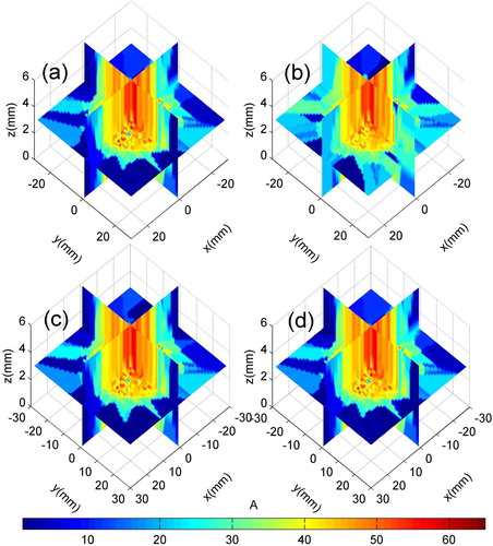
Table 1. SNR and δ_r of reconstruction results of TGSVD and TSVD (noise level r = 10⁻²).

Regularization operator	SNR	δr
In	21.25	8.66%
L1	36.43	1.51%
L2	49.51	0.33%

The results in Table 1 show that the TGSVD method can effectively improve the inaccurate problem in TSVD solution caused by the ill-posedness of arc current reconstruction. Under the noise level of r = 1%, SNR of TGSVD solution is higher than that of TSVD, thus it is able to restore the reference current distribution.

5.2. The numerical results of general-form Tikhonov method

The results of Tikhonov method in standard-form and general-form are shown in Figure 7. It is concluded that the general-form Tikhonov method significantly improved the precision of current reconstructing. The error analyses in Table 2 demonstrate that the utilization of L₁ and L₂ operators enabled the regularization process to overcome the shortcomings of the standard form, and achieved high-quality solutions in spite of ill-posedness. The general-form Tikhonov method reduces the relative error and raises the SNR significantly as expected. Moreover, general-form Tikhonov method leads to smooth solutions which are approximately identical to that of TGSVD method.

Figure 7. Current distribution of arc column section reconstructed by Tikhonov regularization (noise level r = 10⁻²): (a) the reference distribution; (b) standard-form Tikhonov (L = I_n); (c) general-form (L = L₁).

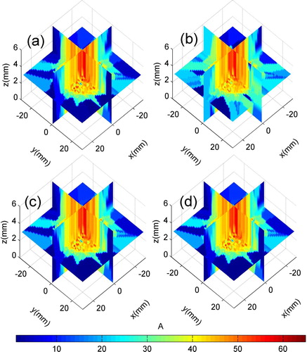
Table 2. SNR and δ_r of Tikhonov regularization (noise level r = 10⁻²).

Regularization operator	SNR	δr
In	21.1864	8.72%
L1	39.0355	1.12%
L2	39.1370	1.10%

5.3. The influence of regularization parameter selection methods

Specifically, general-form Tikhonov regularization is used to study the performance of three regularization parameter selection methods GCV, QO and NCP with the noise r = 1% imposed. Geometric dimensions and mesh generation parameters are the same as the previous example. The selected regularization parameters and corresponding relative error are shown in Table 3.

Table 3. Regularization parameter λ and corresponding relative error δ_r of three parameter-choice methods: GCV, QO and NCP.

Regularization operator	Parameter selection method	λ	SNR	δr
In	GCV	0.1408	21.1864	8.72%
In	QO	5.3663	19.8095	10.22%
In	NCP	2.1118	19.9681	10.04%
L1	GCV	14.4738	39.0355	1.12%
L1	QO	35.7915	34.4192	1.90%
L1	NCP	17.1821	38.8931	1.14%
L2	GCV	2.2391 × 10^3	39.1370	1.10%
L2	QO	3.9290 × 10^4	54.6635	0.18%
L2	NCP	100.5347	26.9391	4.50%

According to Table 3, none of these regularization parameter selection methods can guarantee high quality solutions under the standard format. The GCV and QO criterions are more robust and perform well for L₁ and L₂ operators. The NCP method did not achieve the expected results, especially when using L₂ operator. To analyze the accuracy, the comparison of evaluation index SNR with regard to each method is shown in Figure 8. The range of the noise level is 1%∼10%.

Figure 8. SNR versus noise level with three parameter selection criterions for different regularization operators: (a) standard-form Tikhonov, L = I_n; (b) general-form, L = L₁; (c) general-form, L = L₂.

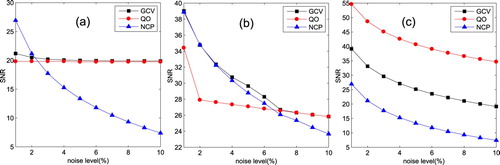
Analyzing Figure 8, it is recommended to use the QO criterion for this problem, especially for larger noise. The method always obtains smooth solutions by choosing very large parameters. Among the other two methods whose performances are more sensitive to the noise level, the GCV criterion is only suitable for L₁ and L₂ operators with relatively low noise imposed. By contrast, the NCP method is more likely to fail in obtaining the effective parameter for larger noise. It can be found that the parameters selected by NCP have little change with the increase of noise, which leads to under-smoothing. Thus for this kind of problem, the L₂ operator with parameter selected by QO criterion is more robust. The test is not sufficient to show which parameter-choice is the favour one, but it is beneficial to try different types of parameter-choice methods for real problems until we find the preferable ones.

6. Conclusions

In this paper, a modified regularization scheme is proposed to reconstruct the current density of a vacuum switching arc by inverting the magnetic data as measured with an array of sensors. The finite element technique is employed to discretize the current region concerning the boundary conditions to approximate the real model. The underdetermined regularization format for GSVD is analyzed. The numerical tests show that incorporating the derivative operators into the regularization process leads to better arc inversion results. The TGSVD and Tikhonov methods behave equivalently. In addition, the effectiveness of GCV, QO and NCP methods on optimizing the regularization parameter has been studied. In the future, a more accurate discrete arc model along with other robust regularization techniques can be developed. And the disturbances of the components in vacuum circuit breakers will be considered to be eliminated. Furthermore, the experimental verification will be used to validate the numerical process.

Acknowledgements

We thank the reviewers and editors for their warm work in the paper revision process. Meanwhile we thank LetPub (www.letpub.com) for its linguistic assistance during the preparation of this manuscript.

Disclosure statement

No potential conflict of interest was reported by the author(s).

Additional information

Funding

This work was supported by the National Natural Science Foundation of China [grant number 51777136].

References

- Debellut E, Gary F, Cajal D, et al. Study of re-strike phenomena in a low-voltage breaking device by means of the magnetic camera. J Phys D Appl Phys. 2001;34:1665–1674. doi: 10.1088/0022-3727/34/11/317
- Brdys C, Toumazet JP, Velleaud G, et al. Study of the low-voltage electric breaking arc restrike by means of an inverse method. IEEE Trans Plasma Sci. 1999;27(2):595–603. doi: 10.1109/27.772291
- Brdys C, Toumazet JP, Laurent A, et al. Optical and magnetic diagnostics of the electric arc dynamics in a low voltage circuit breaker. Meas Sci Technol. 2002;13:1146–1153. doi: 10.1088/0957-0233/13/7/324
- Toumazet JP, Brdys C, Laurent A, et al. Combined use of an inverse method and a voltage measurement: estimation of the arc column volume and its variations. Meas Sci Technol. 2005;16:1525–1533. doi: 10.1088/0957-0233/16/7/015
- Zhang PF, Zhang GG, Dong JL, et al. Non-intrusive magneto-optic detecting system for investigations of air switching arcs. Plasma Sci Technol. 2014;16(7):661–668. doi: 10.1088/1009-0630/16/7/06
- Zhao HC, Liu XM, Wang G. Switching arc inversion based on analysis of electromagnetic characteristics. Rineng. 2019;3:100016.
- Ghezzi L, Piva D, Rienzo LD. Current density reconstruction in vacuum arcs by inverting magnetic field data. IEEE Trans Magn. 2012;48(8):2324–2333. doi: 10.1109/TMAG.2012.2192287
- Dong JL, Zhang GG, Geng YS, et al. Influence of magnetic measurement modeling on the solution of magnetostatic inverse problems applied to current distribution reconstruction in switching air arcs. IEEE Trans Magn. 2018;54(3):1–4. doi: 10.1109/TMAG.2017.2773265
- Dong JL, Zhang GG, Zhang ZQ, et al. Inverse problem solution and regularization parameter selection for current distribution reconstruction in switching arcs by inverting magnetic fields. Math Probl Eng. 2018;2018:7452863. DOI:10.1155/2018/7452863
- Dong JL, Zhang GG, Geng YS, et al. Current distribution reconstruction in low-voltage circuit breakers based on magnetic inverse problem solution considering ferromagnetic splitters. IEEE Trans Magn. 2018;54(10):8001509. doi: 10.1109/TMAG.2018.2858745
- Kress R, Kuhn L, Potthast R. Reconstruction of a current distribution from its magnetic field. Inverse Probl. 2002;18:1127–1146. doi: 10.1088/0266-5611/18/4/312
- Hauer KH, Kuhn L, Potthast R. On uniqueness and non-uniqueness for current reconstruction from magnetic fields. Inverse Probl. 2005;21:955–967. doi: 10.1088/0266-5611/21/3/010
- Hauer KH, Potthast R, Wannert M. Algorithms for magnetic tomography – on the role of a priori knowledge and constraints. Inverse Probl. 2008;24:1–18. doi: 10.1088/0266-5611/24/4/045008
- Potthast R, Kuhn L. On the convergence of the finite integration technique for the anisotropic boundary value problem of magnetic tomography. Math Method Appl Sci. 2003;26:739–757. doi: 10.1002/mma.392
- Ny ML, Chadebec O, Cauffet G. Current distribution identification in fuel cell stacks from external magnetic field measurements. IEEE Trans Magn. 2013;49(5):1925–1928. doi: 10.1109/TMAG.2013.2239967
- Ghasemifard F, Johansson M, Norgren M. Current reconstruction from magnetic field using spherical harmonic expansion to reduce impact of disturbance fields. Inverse Prob Sci Eng. 2017;25(6):795–809. doi: 10.1080/17415977.2016.1201661
- Jeon KW, Lee C, Woo EJ. A harmonic Bz-based conductivity reconstruction method in MREIT with influence of non-transversal current density. Inverse Prob Sci Eng. 2018;26(6):811–833. doi: 10.1080/17415977.2017.1352587
- Marion D, Jérémy H, Stephanie L. Sensitivity analysis for 3D Maxwell’s equations and its use in the resolution of an inverse medium problem at fixed frequency. Inverse Prob Sci Eng. 2019;28(4):459–496.
- Liu J, Sun XS, Meng XH, et al. A novel shape function approach of dynamic load identification for the structures with interval uncertainty. Int J Mech Mater Des. 2016;12(3):375–386. doi: 10.1007/s10999-015-9304-3
- Liu J, Meng XH, Zhang DQ, et al. An efficient method to reduce ill-posedness for structural dynamic load identification. Mech Syst Siganl Pr. 2017;95:273–285. doi: 10.1016/j.ymssp.2017.03.039
- Sun XS, Liu J, Han X, et al. A new improved regularization method for dynamic load identifation. Inverse Prob Sci Eng. 2014;22(7):1062–1076. doi: 10.1080/17415977.2013.854353
- Hansen PC. Regularization, GSVD and truncated GSVD. BIT. 1989;29(3):491–504. doi: 10.1007/BF02219234
- Christensen-Dalsgaard J, Hansen PC, Thompson MJ, et al. Generalized singular value decomposition analysis of helioseismic inversions. Mon Not R Astron Soc. 1993;264(3):541–564. doi: 10.1093/mnras/264.3.541
- Hansen PC. Rank-Deficient and discrete ill-posed problems. Philadelphia (PA): SIAM Press; 1998.
- Noschese S, Reichel L. Some matrix nearness problems suggested by Tikhonov regularization. Linear Algerbra Appl. 2016;502:66–386.
- Huang GX, Noschese S, Reichel L. Regularization matrices determined by matrix nearness problems. Linear Algebra Appl. 2016;502:41–57. doi: 10.1016/j.laa.2015.12.008
- Reichel L, Ye Q. Simple square smoothing regularization operators. Electron T Numer Ana. 2009;33:63–83.
- Hansen PC, Kilmer ME, Kjeldsen RH. Exploiting residual information in the parameter choice for discrete ill-posed problems. BIT. 2006;46:41–59. doi: 10.1007/s10543-006-0042-7