Spectral graph wavelet regularization and adaptive wavelet for the backward heat conduction problem

Abstract

This paper proposes a new regularization technique using spectral graph wavelet for backward heat conduction problem (BHCP) on the graph. The method uses the fourth-order compact difference for an approximation of differential operators. Meanwhile, the error estimate between the exact and wavelet regularized solution is derived. Adaptive node arrangement is obtained using spectral graph wavelet. The essence of the method is that the same operator can be used for the construction of the spectral graph wavelet and the approximation of the differential operator. The proposed method is applied to solve BHCP on graph arising from regular one-dimensional and two-dimensional mesh. Numerical results show that we can obtain a stable solution using spectral graph wavelet regularization. Moreover, spectral graph wavelet adaptivity and fourth-order compact difference scheme lead to a very efficient solution.

Keywords:

• Backward heat conduction problem
• spectral graph wavelet
• regularization
• adaptive node arrangement
• compact difference scheme
• inverse problem
• graph

2010 Mathematics Subject Classifications:

• 35
• 41
• 65

1. Introduction

The inverse problems [1] are those in which one would like to determine causes provided a desired or observed effect is known. The applications include the inverse problem of gravimetry, tomography, the inverse conductivity problem, inverse scattering, inverse spectral problems, etc. Generally, an inverse problem is classified into three types: determination of the boundary conditions [2], identification of the physical parameters or parameter identification [3], determination of the initial state of the system [4, 5]. We deal with the third type of inverse problem in the field of heat transfer, i.e. to find the temperature distribution for 0<t<T from measured temperature distribution at a time t = T>0, called the backward heat conduction problem (BHCP) [6]. The BHCP we consider is (1) $\begin{array}{rl}{u}_t& =\nu \mathrm{△}u\mathrm{in}\Omega ,\\ u& =u_B\mathrm{on}\mathrm{\partial }D\times (0,T),\\ u& =u_F\mathrm{on}D\times \{T\}.\end{array}$(1) Practically, this situation arises where measured temperature distribution in a finite strip is known at some final time T with the known value of temperature across the boundary of the domain. Here, ν is the constant heat diffusion coefficient and $\mathrm{△}$ stands for $\mathrm{k}$-dimensional Laplacian operator. The space–time domain is denoted as $\mathrm{\Omega }=D\times (0,T)$ where D is the bounded domain in $R^{\mathrm{k}}$.

BHCP is ill-posed since it violates the third property in the sense of Hadamard, i.e. the solution does not depend continuously on the final temperature. Moreover, any small disruption in the input data may yield drastic change to the solution. In fact, there is a quick disappearance of the characteristic of the initial temperature due to the rapid decay of temperature with respect to time t. Hence, due to measurement and computational error, the numerical recovery of initial temperature from measured data is a tough task. Such difficulties can be overcome by using some regularization techniques [7].

Now, we brief several methods with different regularization techniques proposed for the BHCP in literature. The mollification method is used in [8] where a sequence of mollification operators is used to mollifying the improper data. The modified boundary element method has been studied in [9]. In [4], iterative Boundary element method (BEM) is used where an iterative algorithm is numerically implemented using BEM and thus reduces the BHCP to a sequence of well-posed forward heat conduction problem. Some other methods include optimal filtering method [10], quasi-reversibility technique [11], kernel-based method [12], operator-splitting method [13] and the method of fundamental solutions [14]. Seeking a group preserving scheme, BHCP has been solved in [5]. The Fourier regularization method has been entrenched in [15] to eliminate all high frequencies from the solution and thus converting them to well-posed. Central difference regularization is discussed in [16].

In articles [5, 16, 17], the authors use standard finite difference scheme for spatial discretization of second derivative for BHCP. Compact difference scheme which is a viable alternative to standard finite difference scheme was first introduced by Lele [18] as a generalization of Padè scheme. Additionally, it is also useful for filtering and interpolation applications to evaluate the derivatives. Compact schemes are a simple and powerful tool to inherit the spectral-like resolution in the evaluation of derivatives of numerical solutions and very low numerical dissipation with the freedom of choosing the complex geometries and boundary conditions. With compact difference scheme, one can obtain numerical solutions with high accuracy without requiring extra boundary conditions which include one of its advantages. Due to smaller stencil size compared to standard finite difference scheme for the same accuracy, the matrices obtained in compact schemes have smaller bandwidth. This results in the low computational cost for compact schemes which adds on to the salient features of this scheme. In recent years, compact scheme has been applied to solve numerous problems like non-linear dispersive wave problem [19], Navier–Stokes equations [20], option pricing problems [21], Reaction–Diffusion problems [22], viscous incompressible flows on non-uniform grids [23] and the numerical solution of PDE (partial differential equation) [24].

The wavelet methods have been used to efficiently solve partial differential equations (PDEs) [25] due to its attractive mathematical properties which include multiscale analysis, wavelet decomposition, fast wavelet transform, vanishing moments, localization and data compression. Due to this useful properties, wavelet methods have been successfully applied to direct as well as inverse problems. For example, Haar wavelet is used by authors in [26, 27] for some direct and inverse problems. Legendre wavelets is used in [28] to solve nonlinear problems, Chebyshev and Hermite wavelet are used in [29, 30]. The numerical solution of some integral equations using wavelets based method can be seen in [31–34]. The application to some other inverse problems includes sideways heat equation [35], the Cauchy problem for the Laplace equation [36], the Cauchy problem for the Helmholtz equation [37] and backward heat conduction problem [38]. The wavelets used until now to solve inverse problems are classical wavelets which are defined on flat geometries. The critical issue is to solve the inverse problems on a general manifold and graph. The spectral graph wavelets [39] (introduced by Hammond et al. in 2011) exhibit good localization properties in the limit of fine scale. Other attractive properties include smoothness, shape-awareness, multiscale, and being flexible and adaptable for complex geometry and arbitrary topology. Moreover, in the construction of this wavelet, the mesh is not required to discretize the domain, hence is well suited for dealing with the inverse problems on general manifold and graph.

While numerically dealing with PDEs, one can either opt static node arrangement [40] or can work with adaptive/dynamic node arrangement [41, 42]. Static node arrangement is formulated at the beginning of the numerical computation where a huge set of nodes are needed to determine all the features of the solution. This continuously growing demands on computation raise the computational as well as storage cost. To overcome these issues, adaptive node arrangement is required where the strategy is to dynamically adapt discretizations in the way of the computational solution process. Instead of dealing with a large set of uniform points in the whole domain, more and more points are added only in the neighbourhood of the solution having sharp features thus leads to the dynamic adaption of the node arrangement. To guide the refinenemt, an indicator function is required for the generation of adaptive node arrangement. In the spectral graph wavelet, the graph Laplacian serves this purpose. While adaptive spectral graph wavelet method (ASGWM) is already applied for solving some linear and non-linear direct problems on the sphere and graph structure [43, 44], it has never been applied to solve inverse problems on general manifold or graph-like structure.

In this paper, we deal with the BHCP on path graph (graph arising from regular one-dimensional mesh) and 2d-grid graph (graph arising from regular two-dimensional mesh). Though, we are dealing here only with a simple graph, BHCP on the complex graph will be considered in the near future. Moreover, in this article, our aim is only to introduce a new regularization technique which can be applied to solve any inverse problem defined on the graph. To the best of our knowledge, there is no regularization technique available in the literature to solve an inverse problem on the graph. The primary contribution of this paper can be seen in the following manner:

• In adaptive spectral graph wavelet method, the same operator, i.e. the approximation of graph laplacian, is used for constructing wavelet as well as for the approximation of second-order differential operator occurred in the PDE.

• Spectral graph wavelet is used for the regularization of BHCP by filtering the high frequency instabilities of the noisy data, thus converting them to well-posed.

• Error estimate between exact and wavelet regularized solution is obtained.

• For the first time, useful properties of the spectral graph wavelet (BHCP in our case) are exploited here to solve the inverse problem on graph arising from the regular mesh.

The paper is organized as follows: a brief description of spectral graph wavelet is given in Section 2. In Section 3, the adaptive spectral graph wavelet method is explained. Second derivative approximation using fourth-order compact difference scheme with its Fourier analysis is also discussed in this section. In Section 4, spectral graph wavelet regularization with the error estimate is given. Some numerical problems are considered in Section 5. The conclusion of the paper with some proposed future work is given in Section 6.

2. Spectral graph wavelet: a brief description

In spectral graph wavelet [39], wavelets are defined on the graph by working in the spectral graph domain, where the basis consists of the eigenfunction of the graph Laplacian $\mathcal{L}$. Classical wavelets which are constructed by translating and dilating a single wavelet cannot be directly extended on the graph as it is not clear how to define translation and dilation on an irregular graph. In this section, a brief description of the spectral graph wavelet defined on the arbitrary finite weighted graph is given.

2.1. Weighted graph

A weighted graph $G=\{E,V,w\}$ consists of a set of vertices V, a set of edges E and a weight function $w:E\to {\mathbb{R}}^{+}$. The weighted function assigns a positive weight to each edge. Suppose the graph is finite (i.e. the number of vertices $|V|=N$ in the graph $<\mathrm{\infty }$). The adjacency matrix $A=\{a_{m,k}\}$ for the weighted graph G is the $N\times N$ matrix where $a_{m,k}=\{\begin{array}{ll}w(e)& \mathrm{if}e\in E\mathrm{connects}\mathrm{vertices}m\mathrm{and}k,\\ 0& \mathrm{otherwise}.\end{array}$ It will be assumed that the graph is undirected, i.e. the adjacency matrix A is symmetric matrix. The possibility of negative weights is not considered.

The degree of each vertex m for a weighed graph is written as $d(m)$. It is defined as the sum of weights of all the edges incident to it, i.e. $d(m)=\sum _m{a}_{m,k}$. A diagonal matrix D is defined with diagonal elements equal to the degrees $d(m)$. Consider a function $f:V\to \mathbb{R}$ on the vertices of the graph G. The value of function f on each vertex defines each coordinate and thus it can be viewed as a vector in ${\mathbb{R}}^N$. Adopting this identification, $f\in {\mathbb{R}}^N$ is written as a function on the vertices of the graph and $f(m)$ as the mth vertex value.

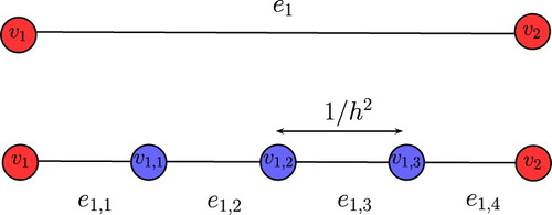
A non-normalized Laplacian is defined as $\mathcal{L}=D-A$. For any function $f\in {\mathbb{R}}^N$, $\mathcal{L}$ can be written as $(\mathcal{L}f)(m)=\sum a_{m,k}.(f(m)-f(k)),$ where the summation is done over all vertices k that are connected to the vertex m. Consider the graph G arising from a regular mesh defined by taking vertices $v_{m,k}$ as points on a regular one-dimensional grid, with each points connected to its two neighbours with weight $\frac{1}{h^2}$ (where h is the distance between adjacent grid points). The graph Laplacian $\mathcal{L}$ to function $f=f_{m,k}$ defined on the vertices is $(\mathcal{L}f{)}_{m.k}=(2f_{m,k}-f_{m,k-1}-f_{m,k+1})/h^2$ which corresponds to standard 3-point stencil approximation of the continuous Beltrami operator with a difference in sign.

In the matrix form, the adjacency matrix A and the matrix D, corresponding to the above mentioned graph G shown in Figure (1) are given by $A=\left[\begin{array}{ccccc}0& {\displaystyle \frac{1}{h^2}}& 0& 0& 0\\ {\displaystyle \frac{1}{h^2}}& 0& {\displaystyle \frac{1}{h^2}}& 0& 0\\ 0& {\displaystyle \frac{1}{h^2}}& 0& {\displaystyle \frac{1}{h^2}}& 0\\ 0& 0& {\displaystyle \frac{1}{h^2}}& 0& {\displaystyle \frac{1}{h^2}}\\ 0& 0& 0& {\displaystyle \frac{1}{h^2}}& 0\end{array}\right],D=\left[\begin{array}{ccccc}{\displaystyle \frac{1}{h^2}}& 0& 0& 0& 0\\ 0& {\displaystyle \frac{2}{h^2}}& 0& 0& 0\\ 0& 0& {\displaystyle \frac{2}{h^2}}& 0& 0\\ 0& 0& 0& {\displaystyle \frac{2}{h^2}}& 0\\ 0& 0& 0& 0& {\displaystyle \frac{1}{h^2}}\end{array}\right].$ Hence, the graph Laplacian $\mathcal{L}$ which is central difference approximation of $-\mathrm{△}$ is written as $\mathcal{L}=\frac{1}{h^2}\left[\begin{array}{ccccc}1& -1& 0& 0& 0\\ -1& 2& -1& 0& 0\\ 0& -1& 2& -1& 0\\ 0& 0& -1& 2& -1\\ 0& 0& 0& -1& 1\end{array}\right].$

Remark 2.1

If vertices $v_{m,k}$ are points on a regular two-dimensional grid (k = 2), with each points connected to its four neighbouring point, then the graph Laplacian $\mathcal{L}$ to function f defined on the vertices is $(\mathcal{L}f{)}_{m.k}=(4f_{m,k}-f_{m,k-1}-f_{m,k+1}-f_{m-1,k}-f_{m+1,k})/h^2$ which corresponds to standard 5-point stencil approximation for $-\mathrm{△}f$.

Figure 1. The graph arising from regular one-dimensional mesh and its discretization.

2.2. Spectral graph wavelet transform (SGWT)

As the graph Laplacian $\mathcal{L}$ is a real symmetric matrix, it has a complete set of orthonormal eigenvectors. Let ${\chi }_l$ $\{l=0,1,2,\dots ,N-1\}$ are the eigenvectors corresponding to the eigenvalues $0={\lambda }_0<{\lambda }_1\le {\lambda }_2\cdots \le {\lambda }_{N-1}$ of the matrix $\mathcal{L}$ (like ${\mathrm{e}}^{\mathrm{i}\omega x}$ used in defining the Fourier transform of the function defined on $\mathbb{R}$ are eigenfunctions of the one–dimensional Laplacian operator $\frac{{\mathrm{d}}^2}{\mathrm{d}{x}^2}$) which satisfy $\mathcal{L}{\chi }_l={\lambda }_l{\chi }_l$.

For any $f\in {\mathbb{R}}^N$ defined on the vertices of the graph G, its graph Fourier transform $\hat{f}$ is defined by (2) $\hat{f}(l)=⟨{\chi }_l,f⟩=\sum _{k=1}^N{\chi }_l^{\ast }(k)f(k),$(2) where the convention is adopted that the inner product be conjugate-linear in the first argument. The inverse graph Fourier transform is (3) $f(k)=\sum _{l=0}^{N-1}\hat{f}(l){\chi }_l(k).$(3) Let $\mathbb{Z}$ denotes the set of integers, then the finite set ${\mathbb{Z}}_N$ can be defined as ${\mathbb{Z}}_N:=\{1,2,\dots ,N\}$. For $f\in l_2({\mathbb{Z}}_N)$ defined on the vertices of graph G, the associated norm is given by $\Vert f{\Vert }_2={(\sum _{k=1}^N|f(k){|}^2)}^{\frac{1}{2}}.$ If we denote $l_2^p({\mathbb{Z}}_N)$ as discrete analogue of Sobolev space $H_p(\mathbb{R})$, then the norm for a function $f\in l_2^p({\mathbb{Z}}_N)$ is given by $\Vert f{\Vert }_p={(\sum _{l=0}^{N-1}(1+l^2{)}^p|\hat{f}(l){|}^2)}^{\frac{1}{2}}.$

Now to define the spectral graph wavelet transform, initially a kernel function $g:{\mathbb{R}}^{+}\to {\mathbb{R}}^{+}$ is chosen satisfying $g(0)=0$ and $\underset{x\to \mathrm{\infty }}{lim}g(x)=0$. The kernel g satisfying these properties is called the wavelet kernel. These assumptions are sufficient for the kernel g to be localized in the spectral domain and the associated spectral graph wavelets will also be localized in the spectral domain. For the wavelet kernel g to be localized in the limit of fine scales, behaviour of g should be monic power of x near the origin [39], i.e. (4) $g(x;\alpha ,\beta ,x_1,x_2)=\{\begin{array}{ll}{x}_1^{-\alpha }{x}^{\alpha }& \mathrm{for}x<x_1\\ s(x)& x_1\le x\le x_2\\ x_2^{\beta }{x}^{-\beta }& \mathrm{for}x>x_2\end{array},$(4) where $g(x_1)=g(x_2)=1$ as g is normalized. The coefficients of the cubic polynomial $s(x)$ are determined by the continuity constraints $s(x_1)=s(x_2)=1$, $s^{\prime }(x_1)=\frac{\alpha }{x_1}$ and $s^{\prime }(x_2)=\frac{\beta }{x_2}$.

For the given spectral graph wavelet kernel g, the wavelet operator $T_g=g(\mathcal{L})$ acts on a given function f by modulating each Fourier mode as (5) $\widehat{T_{g}f}(l)=g({\lambda }_l)\hat{f}(l),$(5) which gives SGWT. The inverse spectral graph wavlet transform (ISGWT) is (6) $(T_{g}f)(m)=\sum _{l=0}^{N-1}g({\lambda }_l)\hat{f}(l){\chi }_l(m).$(6) The wavelet operator at scale $\mathrm{t}$ is then defined by $T_g^{\mathrm{t}}=g(t\mathcal{L})$. It should be noted that even though the spatial domain of the graph is discrete, the domain of the wavelet kernel g is continuous and thus the scaling may be defined for any positive real number $\mathrm{t}$. The spectral graph wavelets are defined as ${\psi }_k^{\mathrm{t}}=T_g^{\mathrm{t}}{\delta }_k,$ where ${\delta }_k$ represents the Kronecker delta vector which takes value 1 at the kth vertex and 0 otherwise, such that ${\psi }_k^{\mathrm{t}}(m)=T_g^{\mathrm{t}}{\delta }_k(m)=\sum _{l=0}^{N-1}g(\mathrm{t}{\lambda }_l){\chi }_l^{\ast }(k){\chi }_l(m).$ The wavelet coefficients of a function f are obtained by taking the inner product of that function with these wavelets, as $W_f(\mathrm{t},k)=⟨{\psi }_k^{\mathrm{t}},f⟩.$ Using the orthonormality of the $\{{\chi }_l\}$, the wavelet coefficients can be achieved directly from the wavelet operators as (7) $W_f(\mathrm{t},k)=(T_g^{\mathrm{t}})(k)=\sum _{l=0}^{N-1}g(\mathrm{t}{\lambda }_l)\hat{f}(l){\chi }_l(k).$(7)

For all numerical computations in this paper, $g(x)$ is choosen according to (4(4) $g(x;\alpha ,\beta ,x_1,x_2)=\{\begin{array}{ll}{x}_1^{-\alpha }{x}^{\alpha }& \mathrm{for}x<x_1\\ s(x)& x_1\le x\le x_2\\ x_2^{\beta }{x}^{-\beta }& \mathrm{for}x>x_2\end{array},$(4) ), where we have taken $s(x)=-5+11x-6x^2+x^3$, $x_1=1,x_2=2$ and $\alpha =\beta =2$, so that (8) $g(x)=\{\begin{array}{ll}{x}^2& \mathrm{for}0<x<1\\ -5+11x-6x^2+x^3& 1\le x\le 2\\ 4x^{-2}& \mathrm{for}x>2\end{array},$(8) One could refer to [39] for other permissible values of $g(x)$.

2.3. Spectral graph scaling function transform (SGST)

Initially, the spectral graph scaling functions ${\varphi }_k=T_{\mathsf{\text{h}}}{\delta }_k=\mathsf{\text{h}}(\mathcal{L}){\delta }_k$ are determined by a single real-valued function $\mathsf{\text{h}}:{\mathbb{R}}^{+}\to \mathbb{R}$ which acts as a low pass filter and satisfies two properties: $\mathsf{\text{h}}(0)>0$ and $\underset{x\to \mathrm{\infty }}{lim}\mathsf{\text{h}}(x)=0$. We will refer to $\mathsf{\text{h}}$ as scaling kernel. In our computation, the chosen scaling kernel is (9) $\mathsf{\text{h}}(\lambda )=\gamma {\mathrm{e}}^{-{\left(\frac{\lambda }{.6{\lambda }_{min}}\right)}^4},$(9) where γ is set such that $\mathsf{\text{h}}(0)=maxg$. The scaling kernel $\mathsf{\text{h}}(\lambda )$ and wavelet kernel $g({\mathrm{t}}_j\lambda )$ for path graph is plotted against λ in Figure 2 with $J=4,{\lambda }_{max}=4.038$. 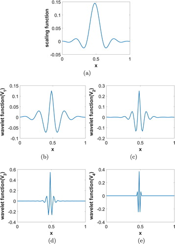The plot of scaling function ${\varphi }_k$ and wavelet function ${\psi }_k^{{\mathrm{t}}_j}$ for the path graph are given in Figure 3 with k is choosen as mid point of the graph. From the figure, the space localization for the wavelets is readily apparent in the limit of fine scale, i.e. as ${\mathrm{t}}_j\to 0$.

Figure 2. The scaling kernel $\mathsf{\text{h}}(\lambda )$ and wavelet generating kernels $g(t_j(\lambda ))$ for $J=4,{\lambda }_{max}=4.038$: (a) $\mathsf{\text{h}}(\lambda )$ and (b) $g(t_j(\lambda ))$.

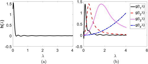
Figure 3. The scaling and wavelet function for J = 4: (a) scaling function, (b) $t_1=9.92$, (c) $t_2=2.89$, (d) $t_3=0.84$, (e) $t_4=0.23$.

The scaling function coefficients are given by (10) $S_f(k)=⟨{\varphi }_k,f⟩.$(10) Note that the scaling functions defined in this way are present merely to smoothly represent the low frequency content of the function f.

Remark 2.2

In spectral graph wavelet, wavelets ψ are not generated through the two-scale relation as for traditional orthogonal wavelets. Therefore, this wavelet will fall under the category of non-MRA wavelet.

2.4. Fast SGWT and fast SGST

The naive way of computing SGWT and SGST, by directly using Equation (7(7) $W_f(\mathrm{t},k)=(T_g^{\mathrm{t}})(k)=\sum _{l=0}^{N-1}g(\mathrm{t}{\lambda }_l)\hat{f}(l){\chi }_l(k).$(7) ) and Equation (10(10) $S_f(k)=⟨{\varphi }_k,f⟩.$(10) ) respectively, requires explicit computation of entire set of eigenvalues and eigenfunctions of the Laplacian operator $\mathcal{L}$. This approach is computationally inefficient for large graphs. 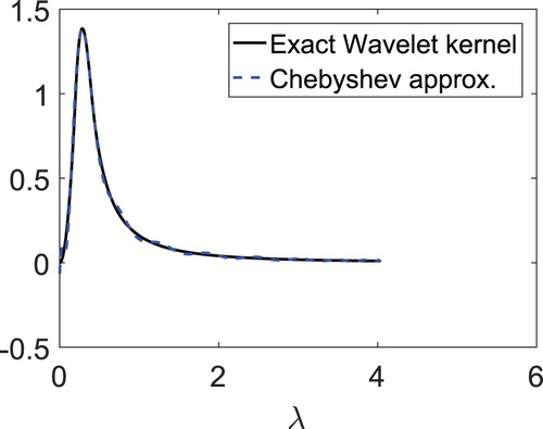A fast transform that avoids the need for computing the complete spectrum of $\mathcal{L}$ is needed for SGWT and SGST to be a useful tool for practical computational problems. In order to achieve this, the wavelet kernel g (discussed in Section 2.2) and the scaling function kernel $\mathsf{\text{h}}$ (discussed in Section 2.3) are approximated by low order polynomials.

The kernels g and $\mathsf{\text{h}}$ are approximated by their Chebyshev polynomials as they form an orthogonal basis for $L_2([-1,1],\frac{\mathrm{d}x}{\sqrt{1-x^2}})$. Any $f\in L_2([-1,1],\frac{\mathrm{d}x}{\sqrt{1-x^2}})$ has a convergent Chebyshev series $f(x)=\frac{1}{2}{e}_0+\sum _{s=1}^{\mathrm{\infty }}{e}_s{T}_s(x),$ with the Chebyshev coefficients $e_s=\frac{2}{\pi }{\int }_{-1}^1\frac{T_s(x)f(x)}{\sqrt{1-x^2}}\mathrm{d}x=\frac{2}{\pi }{\int }_0^{\pi }\cos (s\theta )f(\cos \theta )\mathrm{d}\theta .$ For a fixed wavelet scale ${\mathrm{t}}_j$, approximating $g({\mathrm{t}}_{j}x)$ for $x\in [0,{\lambda }_{max}]$ can be done by shifting the domain using the transformation $y=a(x+1)$ with $a=\frac{{\lambda }_{max}}{2}$. Denoting the shifted Chebyshev polynomials ${\overline{T}}_s(x)=T_s(\frac{x-a}{a})$, we can write (11) $g({\mathrm{t}}_{j}x)=\frac{1}{2}{e}_0^j+\sum _{s=1}^{\mathrm{\infty }}{e}_s^j{\overline{T}}_s(x),$(11) valid for $x\in [0,{\lambda }_{max}]$, with $e_s^j=\frac{2}{\pi }{\int }_0^{\pi }\cos (s\theta )g({\mathrm{t}}_j(a\cos \theta +1))\mathrm{d}\theta .$ For each scale ${\mathrm{t}}_j$, the approximating polynomial $p_j$ is achieved by terminating the Chebyshev expansion given by the equation (11(11) $g({\mathrm{t}}_{j}x)=\frac{1}{2}{e}_0^j+\sum _{s=1}^{\mathrm{\infty }}{e}_s^j{\overline{T}}_s(x),$(11) ) to $M_j$ terms. Exactly the same scheme is used to approximate the scaling function kernel h by the polynomial $p_0$.

The selection of the values of $M_j$ may be considered a design problem, posing a trade off between accuracy and computational cost. The approximate wavelet and scaling function coefficients are given be $\begin{array}{rl}{\tilde{W}}_f({\mathrm{t}}_j,k)& =\frac{1}{2}{e}_0^{j}f(k)+\sum _{s=1}^{M_j}{e}_s^j{\overline{T}}_s(\mathcal{L})f(k),\\ {\tilde{S}}_f(k)& =\frac{1}{2}{e}_0^{0}f(k)+\sum _{s=1}^{M_j}{e}_s^0{\overline{T}}_s(\mathcal{L})f(k).\end{array}$ The plot of the wavelet kernel $g(\lambda )$ and its approximate polynomial $p_4$ for the path graph is plotted in Figure 4.

Figure 4. The wavelet kernel $g({\mathrm{t}}_4\lambda )$ and its approximated polynomial $p_4$ using $M_4=20$.

The spectral graph wavelets depend on the continuous scale parameter $\mathrm{t}$. But for any practical computation, $\mathrm{t}$ must be sampled to a finite number of scales. Choosing J scales $\{{\mathrm{t}}_j{\}}_{j=1}^J$ will yield a collection of NJ wavelets ${\psi }_k^{{\mathrm{t}}_j}={\psi }_k^j$, along with N scaling functions ${\varphi }_k$. Therefore, any function f defined on the vertices of the graph can be written as (12) $f(m)=\sum _{k=1}^N{c}_k{\varphi }_k(m)+\sum _{j=1}^J\sum _{k=1}^N{d}_k^j{\psi }_k^j(m),$(12) where $\{c_k{\}}_{k=1}^N$ are the scaling function coefficients and $\{d_k^j{\}}_{k=1}^N$ are wavelet coefficients at the scale j.

3. Adaptive spectral graph wavelet method (ASGWM)

In this section, we will explain adaptive spectral graph wavelet method to solve BHCP on graph arising from the regular mesh. It should be noted that the graph Laplacian $\mathcal{L}$ can be defined for graphs arising from sampling points on a differential manifold. The graph arising from the regular mesh which we are using is a simple example of such a sampling process. The graph Laplacian $\mathcal{L}$ obtained in the construction of spectral graph wavelet can serve the purpose of the approximation of Laplacian operator. The essence of this method is that the same operator is used for the approximation of the differential operator involved in the differential equation and for the construction of the spectral graph wavelets. We will use fourth-order compact difference approximation (CDA4) for approximating the Laplacian operator.

3.1. Compact difference approximation for second derivative

For a graph arising from regular mesh on an one-dimensional grid (path graph), the value of $\mathrm{k}=1$, hence $\mathrm{△}f=f_{xx}$. Let $x_m=mh$, $t_n=n\tau$ where m and n denote the indices for discrete space and time and h, τ are, respectively, the spatial and temporal variations. Let $(f_{xx}{)}_m$ be second derivative approximation of f at node $x_m$. The compact difference approximation for second derivative at all interior points derived from the formula [18] (13) $\begin{array}{rl}\alpha (f_{xx}{)}_{m-1}+(f_{xx}{)}_m+\alpha (f_{xx}{)}_{m+1}& =a_1\left(\frac{f_{m-1}-2f_m+f_{m+1}}{h^2}\right)\\ & +a_2\left(\frac{f_{m-2}-2f_m+f_{m+2}}{h^2}\right),\end{array}$(13) for $2\le m\le N-1$. For the fourth-order accurate compact finite difference approximation, the coefficients in (13(13) $\begin{array}{rl}\alpha (f_{xx}{)}_{m-1}+(f_{xx}{)}_m+\alpha (f_{xx}{)}_{m+1}& =a_1\left(\frac{f_{m-1}-2f_m+f_{m+1}}{h^2}\right)\\ & +a_2\left(\frac{f_{m-2}-2f_m+f_{m+2}}{h^2}\right),\end{array}$(13) ) are $\alpha =\frac{1}{10},a_1=\frac{6}{5}$ and $a_2=0$ which gives the fourth-order compact difference scheme as follows: (14) $\frac{1}{10}(f_{xx}{)}_{m-1}+(f_{xx}{)}_m+\frac{1}{10}(f_{xx}{)}_{m+1}=\frac{6}{5}\left(\frac{f_{m-1}-2f_m+f_{m+1}}{h^2}\right),2\le m\le N-1.$(14) For boundary points $x_1$ and $x_N$, the fourth-order approximation of second derivative is given by $\begin{array}{rl}(f_{xx}{)}_1+11(f_{xx}{)}_2& =\frac{1}{h^2}(13u{f}_1-27f_2+15f_3-f_4),\\ (f_{xx}{)}_N+11(f_{xx}{)}_{N-1}& =\frac{1}{h^2}(13f_N-27f_{N-1}+15f_{N-2}-f_{N-3}).\end{array}$ The details about compact finite difference scheme with its graphical representation have been discussed in [45].

Remark 3.1

We are using here only fourth-order compact difference scheme for simplicity. In general, one can use any higher order compact difference scheme obtained using (13(13) $\begin{array}{rl}\alpha (f_{xx}{)}_{m-1}+(f_{xx}{)}_m+\alpha (f_{xx}{)}_{m+1}& =a_1\left(\frac{f_{m-1}-2f_m+f_{m+1}}{h^2}\right)\\ & +a_2\left(\frac{f_{m-2}-2f_m+f_{m+2}}{h^2}\right),\end{array}$(13) ).

3.2. Fourier analysis of differencing errors

To compare the difference approximations in numerical analysis, we require additional information to analyse the error characteristics of approximations. Therefore, we study resolution characteristics which can be measured via Fourier analysis/von-Neumann analysis. Resolution characteristics give the measure of error between difference scheme and its exact value over the full grid. Good resolution characteristics mean difference scheme more accurately represents the exact value. We compare above-mentioned approximation for the second derivative with the standard fourth-order finite difference approximation to determine the improvement in error characteristics. One can see [18] for more details about Fourier analysis.

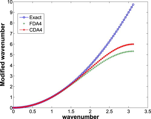
Let ω be wave number ${\omega }^{\mathrm{\prime }\mathrm{\prime }}$ be modified wave number of the difference approximation for second derivative, then the modified wave number for fourth-order compact difference approximation (FDA4) given in (14(14) $\frac{1}{10}(f_{xx}{)}_{m-1}+(f_{xx}{)}_m+\frac{1}{10}(f_{xx}{)}_{m+1}=\frac{6}{5}\left(\frac{f_{m-1}-2f_m+f_{m+1}}{h^2}\right),2\le m\le N-1.$(14) ) (15) ${\omega }^{\mathrm{\prime }\mathrm{\prime }}=-\left[\frac{24{\sin }^2(\omega /2)}{5+\cos (\omega )}\right],$(15) and modified wave number for fourth-order finite difference approximation (CDA4) (16) ${\omega }^{\mathrm{\prime }\mathrm{\prime }}=-[\frac{16}{3}{\sin }^2(\omega /2)-\frac{1}{3}{\sin }^2(\omega )].$(16) The plot for modified wave number of FDA4 and CDA4 with respect to wave number of the exact differentiation (${\omega }^{\mathrm{\prime }\mathrm{\prime }}=-{\omega }^2$) are plotted versus wave number ω in Figure 5. Error in the approximation of the second derivative is measured by the difference between modified wave number for FDA4 and CDA4 with modified wave number of exact differentiation respectively. It is clear from the plot that resolution ability of CDA4 is better than FDA4 since curve of CDA4 remains close to the exact differentiation over relatively vast range of wave number. Note that we are neglecting the negative sign from the expression of modified wavenumbers for plotting the graph.

Figure 5. Plot of modified wave number versus wave number.

3.3. Reconstruction and compression error

For any f defined on the vertices of the graph and a given threshold ε, Equation (12(12) $f(m)=\sum _{k=1}^N{c}_k{\varphi }_k(m)+\sum _{j=1}^J\sum _{k=1}^N{d}_k^j{\psi }_k^j(m),$(12) ) can be written as $f(m)=f_{\ge ϵ}(m)+f_{<ϵ}(m)$, where $f_{\ge ϵ}(m)=\sum _{k=1}^N{c}_k{\varphi }_k(m)+\sum _{j=1}^J\sum _{|d_k^j|\ge ϵ}{d}_k^j{\psi }_k^j(m)\mathrm{and}{f}_{<ϵ}(m)=\sum _{j=1}^J\sum _{|d_k^j|<ϵ}{d}_k^j{\psi }_k^j(m).$$\Vert f-f_{\ge ϵ}\Vert$ is called the compression error and for $ϵ=0$ there is no compression and in that case it is reconstruction error. The number of the node points required for $f_{\ge ϵ}$ is called number of significant coefficients denoted by $N(ϵ)$.

The two test functions which we are considering are:

Test function 1: $f(x)=e^{\frac{-(x-b{)}^2}{c^2}}$ with $b=\frac{1}{3}$ and $c=\frac{1}{8}$ on the interval $[0,1]$.

Test function 2: $f(x,y)={\mathrm{e}}^{-c((x-x_0{)}^2+(y-y_0{)}^2)}$ with c = 1000 and $x_0=y_0=\frac{1}{2}$ in the domain $[0,1]\times [0,1]$.

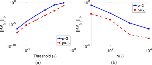
For test function 1, we obtain the following results: for $N=2^7$, the reconstructed function is of order ${10}^{-8}$. The test function $f(x)$ and reconstructed function $f_{\ge ϵ}$ for two different values of ε are given in Figure 6. The plot for compression error $\Vert f-f_{\ge ϵ}\Vert$ versus ε is shown in Figure 7(a). It is clear from the figure that compression error increases with increase in ε. Figure 7(b) shows the plot of compression error versus $N(ϵ)$ from which we can easily observe that compression error decreases with increase in ε.

Figure 6. Test function 1 and reconstructed function for (a) $ϵ={10}^{-1}$ and (b) $ϵ={10}^{-4}.$

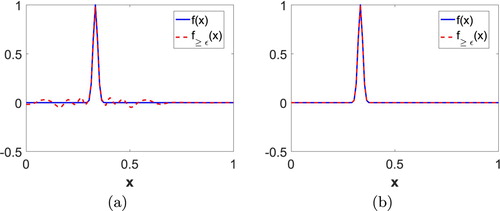
Figure 7. Compression error versus (a) ε and (b) $N(ϵ)$ for test function 1.

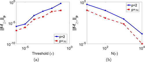
For test function 2, we obtain the following results: for $N=2^7$, the reconstructed function is of order ${10}^{-8}$. In Figure 8, test function 2 and corresponding reconstructed function $f_{\ge ϵ}$ are plotted for different values of ε. The plot for compression error $\Vert f-f_{\ge ϵ}\Vert$ versus ε is shown in Figure 9(a). It is clear from the figure that compression error increases with increase in ε. Figure 9(b) shows the plot of compression error versus $N(ϵ)$ from which we can easily observe that compression error decreases with increase in ε.

Figure 8. Test function 2 and corresponding reconstructed function for different values of ε: (a) test function 2, (b) $f_{\ge ϵ}$ for $ϵ={10}^{-1}$, (c) $f_{\ge ϵ}$ for $ϵ={10}^{-4}$.

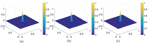
Figure 9. Compression error versus (a) ε and (b) $N(ϵ)$ for test function 2.

3.4. Adaptive node arrangement

The numerical solution of the BHCP is computed by approximating the solution at a discrete set of node points. To discover all the features of the solution, we need a large set of node points, but this will increase the computational as well as storage cost. In some cases, the set which is required to capture all the features of the solution may exceed the practical limitations. To handle with such problem, we work on an adaptive node arrangement. In adaptive node arrangement, the node will keep on modifying according to how the numerical solution of the PDE evolves with time. Instead of taking a larger set of node points, more points are added only in the areas where the solution of PDE has sharp features.

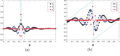
Node adaptation occurs quite naturally in wavelet methods. One of the important properties of wavelets is that the wavelet coefficients $d_k^j$ decreases rapidly for smooth functions. Moreover, if a function has a discontinuity in one of its derivatives then the wavelet coefficients will decrease slowly only near the point of discontinuity and maintains fast decay where the function is smooth. This property of wavelets makes it suitable to detect where in the numerical solution of a partial differential equation shocks or regions with large gradients are located and hence an adaptive node arrangement can be generated. In the case of spectral graph wavelet, if $\{{\mathrm{t}}_j{\}}_{j=1}^J$ is the set of scales, then $d_k^j$ follows the above said fact strictly when j is near J. Hence, we will consider $d_k^J$s (wavelet coefficients at scale ${\mathrm{t}}_J$) for node adaptation. The wavelet coefficient $d_k^j$ at different value of j for two above considered test functions is shown in Figure (10). From the figure, we can see that wavelet coefficients are more localized near non-smooth part of the functions and this localized pattern increases with increase in j.

Figure 10. Wavelet coefficients $d_k^j$ at different value of j for two different test functions: (a) $d_k^j$ for test function 1 and (b) $d_k^j$ for sawtooth function with discontinuity at x = 0.5.

To illustrate the algorithm for node adaptation, we consider a function $f(x)$ defined on a set of node points $x^{old}$ and a pre-defined threshold parameter ε. Perform SGST and SGWT to obtain the set of coefficients $\{c_k{\}}_{k=1}^{|x^{old}|}\cup \{d_k^j{\}}_{j=1,k=1}^{J|x^{old}|}$. We will construct $x^{new}$ (fine node arrangement) from $x^{old}$ (coarse node arrangement). Since each $x_k\in x^{old}$ is associated with a spectral scaling function ${\varphi }_k$, we will keep all the points of $x^{old}$ in $x^{new}$. We recall that every spectral wavelet function at the scale ${\mathrm{t}}_J$, i.e. ${\psi }_k^J$, is uniquely associated with an $x_k\in x^{old}$. We analyse the wavelet coefficients $d_k^J$. If $|d_k^J|\ge ϵ$, then the corresponding node point $x_k\in x^{old}$ is called an active node point. For each active node point $x_k$, an adjacent zone will be added in $x^{new}$. The adjacent zone will serve two purposes:

1. It will make $x^{new}$ finer in the area of sharp features.

2. In solving evolutionary PDEs, additional criteria for node adaptation should be added. In particular, the computational set of node points should consist of node points associated with wavelets whose coefficients are or can possibly become significant during the period of the time when the set of node points remain unchanged.

For an active node point $x_k$, we fix two positive numbers R and M called adjacent zone constants. In the region $\Vert (x-x_k){\Vert }_2\le R$, we obtain M points simulating on the neighbourhood of $x_k$. This will be called the adjacent zone of the point $x_k$.

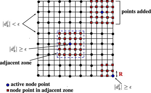
The graphical representation of adaptive grid generation for one and two-dimensional cases is shown in Figures 11 and 12 respectively. For example, as shown in Figure 11, for an active node point with M = 2, we have added two points in the adjacent zone. The process of spectral graph wavelet based adaptive node arrangement generation is as follows:

$x^{new}$ = AdaptiveNodeArrangement(f, $x^{old}$)

• Choose a threshold parameter ε and positive adjacent zone constants R and M.

• m = 0, $x^m=x^{old}$, $f^m=f$.

• do while m = 0 or $x^m\ne x^{m-1}$

  	$-$	Perform SGWT on $f^m$ to get $\{d_k^J{\}}_{k=1}^{|x^m|}$.
  	$-$	$x^{m+1}=x^m$.
  	$-$	Analyse wavelet coefficients $\{d_k^J{\}}_{k=1}^{|x^m|}$ and collect all the active node points.
  	$-$	Corresponding to each active node point, add an adjacent zone in $x^{m+1}$.
  	$-$	Interpolate $f^m$ onto new grid $x^{m+1}$ and call it $f^{m+1}$.
  	$-$	m = m + 1.

• $x^{new}=x^m$.

Figure 11. Adaptive node generation for path graph.

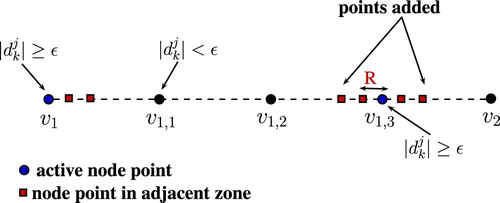
Figure 12. Adaptive node generation for 2-d grid graph.

The adaptive node arrangement for two different test functions in one dimension using the algorithm mentioned above is shown in Figure 13(a,b). In Figure 14, test function 2 and corresponding adaptive node arrangement are plotted.

Figure 13. Functions and the corresponding adaptive node arrangements in one-dimensional setting for R = 0.1 and M = 6. (a) Test function 1, (b) Sawtooth function with discontinuity at x = 0.5.

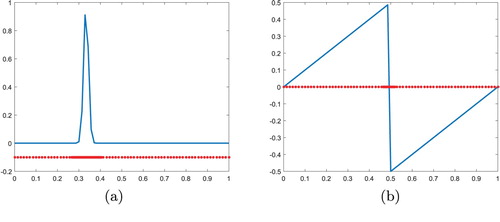
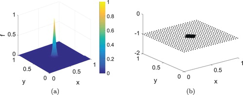
Figure 14. Function and the corresponding adaptive node arrangement in two-dimensional setting for R = 0.1 and M = 6: (a) Test function 2 and (b) adaptive grid.

4. Wavelet regularization

In order to obtain the stable numerical solution for BHCP, we have to apply an appropriate regularization technique. Filtering technique is one of the regularization techniques for constructing the good approximate solution from a severely ill-posed problem. It is very popular due to its ease of implementation (especially in Fourier domain), effectiveness and possibility of obtaining the good approximate solution for ill-posed PDEs. Filtering can be done either in the spatial domain (spatial filtering) or Fourier domain (Fourier filtering) by filtering short wave modes participate in numerical calculations. In filtering technique, the solution is obtained by completely eliminating or suppressing the spurious errors which present in high frequency component of the data. Some of the filtering techniques for ill-posed problems are discussed in [46]. The key disadvantage of Fourier filtering [15] is that the Fourier bases are only localized in the frequency domain yet having global support in the spatial domain. Therefore, they are not efficient in encoding the local signal information. A popular and powerful solution is to use wavelet bases, which are functions localized in both space and frequency. Thus it can capture local signal information in a more efficient and compact way. In this article, we will use spectral graph wavelet as a regularization technique for filtering of high frequency.

Let ${\mathbf{u}}_m(t)$ represents the approximated value of $u(x,t)$ at node $x_m$ for any t>0. By using central difference approximation for second derivative $u_{xx}$ and denoting $u_F=\mathrm{\Phi }$, the difference equation for the one-dimensional backward heat equation (1(1) $\begin{array}{rl}{u}_t& =\nu \mathrm{△}u\mathrm{in}\Omega ,\\ u& =u_B\mathrm{on}\mathrm{\partial }D\times (0,T),\\ u& =u_F\mathrm{on}D\times \{T\}.\end{array}$(1) ) is (17) $\begin{array}{rl}({\mathbf{u}}_m{)}_t(t)& =\nu \frac{{\mathbf{u}}_{m-1}(t)-2{\mathbf{u}}_m(t)+{\mathbf{u}}_{m+1}(t)}{h^2},2\le m\le N-1,\\ {\mathbf{u}}_m(T)& =\mathrm{\Phi }(m),\end{array}$(17) with $\mathbf{u}=({\mathbf{u}}_1(t),{\mathbf{u}}_2(t),\dots ,{\mathbf{u}}_N(t))$ as a vector and boundary conditions ${\mathbf{u}}_1(t)={\mathbf{u}}_N(t)=0$. On the real line, the eigenvector for the one-dimensional Laplacian operator is the complex exponentials ${\mathrm{e}}^{2\pi ilhm}$, thus Fourier and inverse Fourier transform will be (18) $\begin{array}{rl}\hat{f}(l)& =\sum _{m=1}^{M}f(m){\mathrm{e}}^{-2\pi ilhm},\end{array}$(18) (19) $\begin{array}{rl}f(m)& =\sum _{l=0}^{\mathrm{\infty }}\hat{f}(l){\mathrm{e}}^{2\pi ilhm},\end{array}$(19) where $m=\frac{x_m}{h}$. Putting $2\pi lh=\omega$ as scaled wave number, (18(18) $\begin{array}{rl}\hat{f}(l)& =\sum _{m=1}^{M}f(m){\mathrm{e}}^{-2\pi ilhm},\end{array}$(18) ) and (19(19) $\begin{array}{rl}f(m)& =\sum _{l=0}^{\mathrm{\infty }}\hat{f}(l){\mathrm{e}}^{2\pi ilhm},\end{array}$(19) ) become (20) $\begin{array}{rl}\hat{f}(l)& =\sum _{m=1}^{N}f(m){\mathrm{e}}^{-\mathrm{i}\omega m},\end{array}$(20) (21) $\begin{array}{rl}f(m)& =\sum _{l=0}^{\mathrm{\infty }}\hat{f}(l){\mathrm{e}}^{\mathrm{i}\omega m},\end{array}$(21) where ${\mathrm{e}}^{\mathrm{i}\omega m}$ is the Fourier mode. If we consider one particular mode ω in (21(21) $\begin{array}{rl}f(m)& =\sum _{l=0}^{\mathrm{\infty }}\hat{f}(l){\mathrm{e}}^{\mathrm{i}\omega m},\end{array}$(21) ) and put ${\mathbf{u}}_m(t)=\hat{\mathbf{u}}(l,t){\mathrm{e}}^{\mathrm{i}\omega m}$ in (17(17) $\begin{array}{rl}({\mathbf{u}}_m{)}_t(t)& =\nu \frac{{\mathbf{u}}_{m-1}(t)-2{\mathbf{u}}_m(t)+{\mathbf{u}}_{m+1}(t)}{h^2},2\le m\le N-1,\\ {\mathbf{u}}_m(T)& =\mathrm{\Phi }(m),\end{array}$(17) ) for $2\le m\le N-1$, we obtain (22) ${\hat{\mathbf{u}}}_t(l,t)=\nu \hat{\mathbf{u}}(l,t)\left(\frac{{\mathrm{e}}^{\mathrm{i}\omega }-2+{\mathrm{e}}^{-\mathrm{i}\omega }}{h^2}\right),$(22) with (23) $\hat{\mathbf{u}}(l,T)=\hat{\mathrm{\Phi }}(l).$(23) Solving (22(22) ${\hat{\mathbf{u}}}_t(l,t)=\nu \hat{\mathbf{u}}(l,t)\left(\frac{{\mathrm{e}}^{\mathrm{i}\omega }-2+{\mathrm{e}}^{-\mathrm{i}\omega }}{h^2}\right),$(22) ), we get (24) ${\hat{\mathbf{u}}}_t(l,t)=(-4si{n}^2(\omega /2))\frac{\nu \hat{\mathbf{u}}(l,t)}{h^2}.$(24) From (24(24) ${\hat{\mathbf{u}}}_t(l,t)=(-4si{n}^2(\omega /2))\frac{\nu \hat{\mathbf{u}}(l,t)}{h^2}.$(24) ), we observe that $-4si{n}^2(\omega /2)$ is nothing but modified wave number ${\omega }^{\mathrm{\prime }\mathrm{\prime }}$ for finite difference approximation.

Finally, the solution for problem (17(17) $\begin{array}{rl}({\mathbf{u}}_m{)}_t(t)& =\nu \frac{{\mathbf{u}}_{m-1}(t)-2{\mathbf{u}}_m(t)+{\mathbf{u}}_{m+1}(t)}{h^2},2\le m\le N-1,\\ {\mathbf{u}}_m(T)& =\mathrm{\Phi }(m),\end{array}$(17) ) in spectral domain can be obtained by solving (24(24) ${\hat{\mathbf{u}}}_t(l,t)=(-4si{n}^2(\omega /2))\frac{\nu \hat{\mathbf{u}}(l,t)}{h^2}.$(24) ) together with (23(23) $\hat{\mathbf{u}}(l,T)=\hat{\mathrm{\Phi }}(l).$(23) ) which gives (25) $\hat{\mathbf{u}}(l,t)={\mathrm{e}}^{\frac{4\nu {\sin }^2(\omega /2)(T-t)}{h^2}}\hat{\mathrm{\Phi }}(l).$(25) Similarly, if fourth-order compact difference approximation is used instead of finite difference approximation, (22(22) ${\hat{\mathbf{u}}}_t(l,t)=\nu \hat{\mathbf{u}}(l,t)\left(\frac{{\mathrm{e}}^{\mathrm{i}\omega }-2+{\mathrm{e}}^{-\mathrm{i}\omega }}{h^2}\right),$(22) ) can be written as (26) $\hat{\mathbf{u}}(l,t)={\mathrm{e}}^{\frac{24\nu (T-t){\sin }^2(\omega /2)}{h^2(5+cos(\omega ))}}\hat{\mathrm{\Phi }}(l),$(26) where approximation of Laplacian operator is obtained using CDA4 given in (14(14) $\frac{1}{10}(f_{xx}{)}_{m-1}+(f_{xx}{)}_m+\frac{1}{10}(f_{xx}{)}_{m+1}=\frac{6}{5}\left(\frac{f_{m-1}-2f_m+f_{m+1}}{h^2}\right),2\le m\le N-1.$(14) ). Equivalently, (27) ${\mathbf{u}}_m(t)=\sum _{l=0}^{\mathrm{\infty }}{\mathrm{e}}^{\mathrm{i}\omega m}{\mathrm{e}}^{\frac{24\nu (T-t){\sin }^2(\omega /2)}{h^2(5+cos(\omega ))}}\hat{\mathrm{\Phi }}(l).$(27) Moreover, for t = 0, we can easily see from (26(26) $\hat{\mathbf{u}}(l,t)={\mathrm{e}}^{\frac{24\nu (T-t){\sin }^2(\omega /2)}{h^2(5+cos(\omega ))}}\hat{\mathrm{\Phi }}(l),$(26) ) that (28) ${\hat{\mathbf{u}}}_0(l)={\mathrm{e}}^{\frac{24\nu T{\sin }^2(\omega /2)}{h^2(5+cos(\omega ))}}\hat{\mathrm{\Phi }}(l).$(28) The SGWT and ISGWT for a given function f can be written as (29) $\begin{array}{rl}\hat{T_g^{{\mathrm{t}}_j}f}(l)& =\sum _{m=1}^{N}g(t_j{\lambda }_l)f(m){\mathrm{e}}^{-\mathrm{i}\omega m},\end{array}$(29) (30) $\begin{array}{rl}(T_g^{{\mathrm{t}}_j}f)(m)& =\sum _{l=0}^{N-1}g(t_j{\lambda }_l)\hat{f}(l){\mathrm{e}}^{\mathrm{i}\omega m},\end{array}$(30) where $\omega =2\pi lh$. Choose $h=\frac{1}{2(N-1)}$ so that scaled wave number $\omega \in [0,\pi ]$.

Practically, we can never have completely accurate data Φ since it depends on (physical) observations. Thus the data available to us are measured data ${\mathrm{\Phi }}^{\delta }$, so it is perturbed with noise because of the errors in the measurements and the limitations of the measuring instruments. Using (29(29) $\begin{array}{rl}\hat{T_g^{{\mathrm{t}}_j}f}(l)& =\sum _{m=1}^{N}g(t_j{\lambda }_l)f(m){\mathrm{e}}^{-\mathrm{i}\omega m},\end{array}$(29) ) and (30(30) $\begin{array}{rl}(T_g^{{\mathrm{t}}_j}f)(m)& =\sum _{l=0}^{N-1}g(t_j{\lambda }_l)\hat{f}(l){\mathrm{e}}^{\mathrm{i}\omega m},\end{array}$(30) ), the spectral graph wavelet solution ${\mathbf{u}}_J^{\delta }(.,t)$ with measured data ${\mathrm{\Phi }}^{\delta }$ in spectral domain will be (31) ${\hat{\mathbf{u}}}_J^{\delta }(l,t)={\mathrm{e}}^{\frac{24\nu (T-t){\sin }^2(\omega /2)}{h^2(5+cos(\omega ))}}g(t_J{\lambda }_l){\hat{\mathrm{\Phi }}}^{\delta }(l),$(31) or equivalently, the wavelet regularized approximate solution ${\mathbf{u}}_{J,m}^{\delta }(t)$ is (32) ${\mathbf{u}}_{J,m}^{\delta }(t)=\sum _{l=0}^{N-1}{\mathrm{e}}^{\mathrm{i}\omega m}{\mathrm{e}}^{\frac{24\nu (T-t){\sin }^2(\omega /2)}{h^2(5+cos(\omega ))}}g(t_J{\lambda }_l){\hat{\mathrm{\Phi }}}^{\delta }(l).$(32)

Lemma 4.1

The unique solution for the semi discrete problem (17(17) $\begin{array}{rl}({\mathbf{u}}_m{)}_t(t)& =\nu \frac{{\mathbf{u}}_{m-1}(t)-2{\mathbf{u}}_m(t)+{\mathbf{u}}_{m+1}(t)}{h^2},2\le m\le N-1,\\ {\mathbf{u}}_m(T)& =\mathrm{\Phi }(m),\end{array}$(17) ) can be obtained if and only if (33) $\sum _{l=0}^{\mathrm{\infty }}{|{\mathrm{e}}^{\frac{24\nu T{\sin }^2(\omega /2)}{h^2(5+cos(\omega ))}}\hat{\mathrm{\Phi }}(l)|}^2<\mathrm{\infty }.$(33)

Proof.

As already stated earlier, the exact solution u for the problem 17(17) $\begin{array}{rl}({\mathbf{u}}_m{)}_t(t)& =\nu \frac{{\mathbf{u}}_{m-1}(t)-2{\mathbf{u}}_m(t)+{\mathbf{u}}_{m+1}(t)}{h^2},2\le m\le N-1,\\ {\mathbf{u}}_m(T)& =\mathrm{\Phi }(m),\end{array}$(17) can be written in the frequency domain as (34) ${\mathbf{u}}_m(t)=\sum _{l=0}^{\mathrm{\infty }}{\mathrm{e}}^{\mathrm{i}\omega m}{\mathrm{e}}^{\frac{24\nu (T-t){\sin }^2(\omega /2)}{h^2(5+cos(\omega ))}}\hat{\mathrm{\Phi }}(l),$(34) with its Fourier coefficients $\hat{\mathbf{u}}(l,t)={\mathrm{e}}^{\frac{24\nu (T-t){\sin }^2(\omega /2)}{h^2(5+cos(\omega ))}}\hat{\mathrm{\Phi }}(l).$ At t = 0, it becomes ${\hat{\mathbf{u}}}_0(l)={\mathrm{e}}^{\frac{24\nu T{\sin }^2(\omega /2)}{h^2(5+cos(\omega ))}}\hat{\mathrm{\Phi }}(l),$ which implies that (35) $\Vert \mathbf{u}(.,0){\Vert }_2^2=\sum _{l=0}^{\mathrm{\infty }}{|{\hat{\mathbf{u}}}_0(l)|}^2=\sum _{l=0}^{\mathrm{\infty }}{|{\mathrm{e}}^{\frac{24\nu T{\sin }^2(\omega /2)}{h^2(5+cos(\omega ))}}\hat{\mathrm{\Phi }}(l)|}^2.$(35) Using the condition (33(33) $\sum _{l=0}^{\mathrm{\infty }}{|{\mathrm{e}}^{\frac{24\nu T{\sin }^2(\omega /2)}{h^2(5+cos(\omega ))}}\hat{\mathrm{\Phi }}(l)|}^2<\mathrm{\infty }.$(33) ), we obtain (36) $\Vert u(.,0){\Vert }_2^2<\mathrm{\infty }.$(36) Now we define the vector ρ with ${\rho }_m$ as ${\rho }_m=\sum _{l=0}^{\mathrm{\infty }}{\mathrm{e}}^{\mathrm{i}\omega m}{\mathrm{e}}^{\frac{24\nu T{\sin }^2(\omega /2)}{h^2(5+cos(\omega ))}}\hat{\mathrm{\Phi }}(l),$ so that ρ $\in l_2(D)$ and (37) $\hat{\rho }(l)={\mathrm{e}}^{\frac{24\nu T{\sin }^2(\omega /2)}{h^2(5+cos(\omega ))}}\hat{\mathrm{\Phi }}(l).$(37) Now consider the direct semi discrete problem (38) $\begin{array}{rl}({\mathbf{u}}_m{)}_t(t)& =\nu \frac{{\mathbf{u}}_{m-1}(t)-2{\mathbf{u}}_m(t)+{\mathbf{u}}_{m+1}(t)}{h^2},2\le m\le N-1,\\ {\mathbf{u}}_m(0)& ={\rho }_m,\end{array}$(38) with ${\mathbf{u}}_1(t)={\mathbf{u}}_N(t)=0$. The problem (38(38) $\begin{array}{rl}({\mathbf{u}}_m{)}_t(t)& =\nu \frac{{\mathbf{u}}_{m-1}(t)-2{\mathbf{u}}_m(t)+{\mathbf{u}}_{m+1}(t)}{h^2},2\le m\le N-1,\\ {\mathbf{u}}_m(0)& ={\rho }_m,\end{array}$(38) ) is the direct problem which has a unique solution, say $\mathbf{u}$. We can write the solution for (38(38) $\begin{array}{rl}({\mathbf{u}}_m{)}_t(t)& =\nu \frac{{\mathbf{u}}_{m-1}(t)-2{\mathbf{u}}_m(t)+{\mathbf{u}}_{m+1}(t)}{h^2},2\le m\le N-1,\\ {\mathbf{u}}_m(0)& ={\rho }_m,\end{array}$(38) ) as (39) ${\mathbf{u}}_m(t)=\sum _{l=0}^{\mathrm{\infty }}{\mathrm{e}}^{\mathrm{i}\omega m}{\mathrm{e}}^{\frac{-24\nu t{\sin }^2(\omega /2)}{h^2(5+cos(\omega ))}}\hat{\rho }(l).$(39) Putting t = T in (39(39) ${\mathbf{u}}_m(t)=\sum _{l=0}^{\mathrm{\infty }}{\mathrm{e}}^{\mathrm{i}\omega m}{\mathrm{e}}^{\frac{-24\nu t{\sin }^2(\omega /2)}{h^2(5+cos(\omega ))}}\hat{\rho }(l).$(39) ) and using (37(37) $\hat{\rho }(l)={\mathrm{e}}^{\frac{24\nu T{\sin }^2(\omega /2)}{h^2(5+cos(\omega ))}}\hat{\mathrm{\Phi }}(l).$(37) ), we get $\begin{array}{rl}{\mathbf{u}}_m(T)& =\sum _{l=0}^{\mathrm{\infty }}{\mathrm{e}}^{\mathrm{i}\omega m}{\mathrm{e}}^{\frac{-24\nu T{\sin }^2(\omega /2)}{h^2(5+cos(\omega ))}}\hat{\rho }(l)\\ & =\sum _{l=0}^{\mathrm{\infty }}{\mathrm{e}}^{\frac{-24\nu T{\sin }^2(\omega /2)}{h^2(5+cos(\omega ))}}({\mathrm{e}}^{\frac{24\nu T{\sin }^2(\omega /2)}{h^2(5+cos(\omega ))}}\hat{\mathrm{\Phi }}(l)){\mathrm{e}}^{\mathrm{i}\omega m}\\ & =\sum _{l=0}^{\mathrm{\infty }}\hat{\mathrm{\Phi }}(l){\mathrm{e}}^{\mathrm{i}wm}=\mathrm{\Phi }(m).\end{array}$ This proves that problem (17(17) $\begin{array}{rl}({\mathbf{u}}_m{)}_t(t)& =\nu \frac{{\mathbf{u}}_{m-1}(t)-2{\mathbf{u}}_m(t)+{\mathbf{u}}_{m+1}(t)}{h^2},2\le m\le N-1,\\ {\mathbf{u}}_m(T)& =\mathrm{\Phi }(m),\end{array}$(17) ) has a unique solution.

The localization result for kernels g which have a zero of integer multiplicity at the origin will be given by the following lemma. Such kernels can be approximated by a single monomial for small scales.

Lemma 4.2

Let g be $(K+1)$ times continuously differentiable, satisfying $g(0)=0,$ $g^{(r)}=0$ for all $r<K,$ and $g^{(K)}(0)=C\ne 0$. Assume that there is some $t^{\prime }\ge 0$ such that $|g^{(K+1)}(\lambda )|\le b$ for all $\lambda \in [0,t^{\prime }{\lambda }_{N-1}]$. Then, for $\tilde{g}(t\lambda )=(C/K!)(t\lambda {)}^K,$ we have $M(t)=\underset{\lambda \in [0,{\lambda }_{N-1}]}{sup}|g(t\lambda )-\tilde{g}(t\lambda )|\le t^{K+1}\frac{{\lambda }_{N-1}^{K+1}}{(K+1)!}b$

Proof.

For detail about the proof, one can refer to [39].

Theorem 4.1

Let g be a kernel satisfying the hypothesis of Lemma 4.2, with constant $t^{\prime }$ and b. Then for a given exact data $\mathrm{\Phi }(x),$ the wavelet regularized solution ${\mathit{u}}_J$ as defined by (32(32) ${\mathbf{u}}_{J,m}^{\delta }(t)=\sum _{l=0}^{N-1}{\mathrm{e}}^{\mathrm{i}\omega m}{\mathrm{e}}^{\frac{24\nu (T-t){\sin }^2(\omega /2)}{h^2(5+cos(\omega ))}}g(t_J{\lambda }_l){\hat{\mathrm{\Phi }}}^{\delta }(l).$(32) ) continuously depends on $\mathrm{\Phi }(x)$ in $C([0,T];L_2(\Omega ))$. Furthermore, we have (40) $\Vert {\mathit{u}}_J-{\mathit{u}}_J^{\delta }{\Vert }_2\le a{\mathrm{e}}^{\frac{6\nu (T-t)}{h^2}}{2}^{-JK}\delta$(40)

Proof.

Let ${\mathbf{u}}_J$ and ${\mathbf{w}}_J$ are two solutions of (32(32) ${\mathbf{u}}_{J,m}^{\delta }(t)=\sum _{l=0}^{N-1}{\mathrm{e}}^{\mathrm{i}\omega m}{\mathrm{e}}^{\frac{24\nu (T-t){\sin }^2(\omega /2)}{h^2(5+cos(\omega ))}}g(t_J{\lambda }_l){\hat{\mathrm{\Phi }}}^{\delta }(l).$(32) ) corresponding to the final values Φ and ψ respectively. From (32(32) ${\mathbf{u}}_{J,m}^{\delta }(t)=\sum _{l=0}^{N-1}{\mathrm{e}}^{\mathrm{i}\omega m}{\mathrm{e}}^{\frac{24\nu (T-t){\sin }^2(\omega /2)}{h^2(5+cos(\omega ))}}g(t_J{\lambda }_l){\hat{\mathrm{\Phi }}}^{\delta }(l).$(32) ), we have (41) $\begin{array}{rl}{\mathbf{u}}_{J,m}^{\delta }(t)& =\sum _{l=0}^{N-1}{\mathrm{e}}^{\mathrm{i}\omega m}{\mathrm{e}}^{\frac{24\nu (T-t){\sin }^2(\omega /2)}{h^2(5+cos(\omega ))}}g(t_J{\lambda }_l)\hat{\mathrm{\Phi }}(l),\end{array}$(41) (42) $\begin{array}{rl}{\mathbf{w}}_{J,m}^{\delta }(t)& =\sum _{l=0}^{N-1}{\mathrm{e}}^{\mathrm{i}\omega m}{\mathrm{e}}^{\frac{24\nu (T-t){\sin }^2(\omega /2)}{h^2(5+cos(\omega ))}}g(t_J{\lambda }_l)\hat{\psi }(l).\end{array}$(42) $\begin{array}{rl}\Vert {\mathbf{u}}_J-{\mathbf{w}}_J{\Vert }_2& =\Vert {\hat{\mathbf{w}}}_J-{\hat{\mathbf{u}}}_J{\Vert }_2\\ & ={\left[\sum _{l=0}^{N-1}{({\mathrm{e}}^{\frac{24\nu (T-t){\sin }^2(\omega /2)}{h^2(5+cos(\omega ))}}g(t_J{\lambda }_l)\hat{\mathrm{\Phi }}(l)-{\mathrm{e}}^{\frac{24\nu (T-t){\sin }^2(\omega /2)}{h^2(5+cos(\omega ))}}g(t_J{\lambda }_l)\hat{\psi }(l))}^2\right]}^{\frac{1}{2}}\\ & =\underset{l}{sup}|{\mathrm{e}}^{\frac{24\nu (T-t){\sin }^2(\omega /2)}{h^2(5+cos(\omega ))}}g(t_J{\lambda }_l)|{(\sum _{l=0}^{N-1}|\hat{\mathrm{\Phi }}(l)-\hat{\psi }(l){|}^2)}^{\frac{1}{2}}\\ & =\underset{l}{sup}|{\mathrm{e}}^{\frac{24\nu (T-t){\sin }^2(\omega /2)}{h^2(5+cos(\omega ))}}g(t_J{\lambda }_l)|\Vert \hat{\mathrm{\Phi }}-\hat{\psi }{\Vert }_2\\ & \le \underset{l}{sup}B(l)\Vert \hat{\mathrm{\Phi }}-\hat{\psi }{\Vert }_2,\end{array}$ where $B(l):=|{\mathrm{e}}^{\frac{24\nu (T-t){\sin }^2(\omega /2)}{h^2(5+cos(\omega ))}}g(t_J{\lambda }_l)|.$

Now we choose $g(t_J{\lambda }_l)$ as (43) $g(t_J{\lambda }_l)=\{\begin{array}{ll}{\displaystyle \frac{C}{K!}}(t_J{\lambda }_l{)}^K,& 0\le \lambda \le N-1\\ 0,& \mathrm{otherwise}\end{array},$(43) so that $\begin{array}{rl}\underset{l}{sup}B(l)& =\underset{l}{sup}|{\mathrm{e}}^{\frac{24\nu (T-t){\sin }^2(\omega /2)}{h^2(5+cos(\omega ))}}\frac{C}{K!}(t_J{\lambda }_l{)}^K|\\ & \le {\mathrm{e}}^{\frac{6\nu (T-t)}{h^2}}\underset{\lambda \in [0,{\lambda }_{N-1}]}{sup}\frac{C}{K!}(t_J{\lambda }_l{)}^K\\ & \le {\mathrm{e}}^{\frac{6\nu (T-t)}{h^2}}\frac{C}{K!}(t_J{\lambda }_{N-1}{)}^K.\end{array}$ Now we choose the scales for wavelets as $t_j=2^{-j}$ for $j\in [1,2,\dots ,J]$ and $a=\frac{C}{K!}{\lambda }_{N-1}$, then we get $\underset{l}{sup}B(l)\le a{\mathrm{e}}^{\frac{6\nu (T-t)}{h^2}}{2}^{-JK}.$ Hence, (44) $\Vert {\mathbf{u}}_J-{\mathbf{w}}_J{\Vert }_2\le a{\mathrm{e}}^{\frac{6\nu (T-t)}{h^2}}{2}^{-JK}\Vert \hat{\mathrm{\Phi }}-\hat{\psi }{\Vert }_2.$(44) This completes the proof of the theorem.

Furthermore, using (44(44) $\Vert {\mathbf{u}}_J-{\mathbf{w}}_J{\Vert }_2\le a{\mathrm{e}}^{\frac{6\nu (T-t)}{h^2}}{2}^{-JK}\Vert \hat{\mathrm{\Phi }}-\hat{\psi }{\Vert }_2.$(44) ) and the condition $\Vert \mathrm{\Phi }-{\mathrm{\Phi }}^{\delta }{\Vert }_2\le \delta$, we have (45) $\Vert {\mathbf{u}}_J-{\mathbf{u}}_J^{\delta }{\Vert }_2\le a{\mathrm{e}}^{\frac{6\nu (T-t)}{h^2}}{2}^{-JK}\delta .$(45)

Error estimate

Next, we will prove the error estimate between the exact solution and wavelet regularized solution for BHCP.

Theorem 4.2

Let $\mathbf{u}$ be the solution using exact data Φ and ${\mathbf{u}}_J^{\delta }$ be the wavelet regularized solution using measured data ${\mathrm{\Phi }}^{\delta }$. Assume that there exists a priori bound $\Vert {\mathbf{u}}_0{\Vert }_2\le E$ and $\Vert \mathrm{\Phi }-{\mathrm{\Phi }}^{\delta }{\Vert }_2\le \delta$. Let g be a kernel satisfying the hypothesis of Lemma (4.2, with constant $t^{\prime }$ and b. If we choose $h=\frac{1}{2(N-1)}$ with $N=\left[\sqrt{\frac{\ln (E/\delta {)}^{1/T}}{24\nu }}\right]+1,J=[\frac{1}{K}{\log }_2{\left(\frac{E}{\delta }\right)}^{t/T}],$ where $[\cdot ]$ denotes the largest integer part of the real number, then we obtain the following error estimate: (46) $\Vert \mathbf{u}-{\mathbf{u}}_J^{\delta }{\Vert }_2\le E^{1-\frac{t}{T}}{\delta }^{\frac{t}{T}}(2+a{E}^{-\frac{t}{T}}{\delta }^{\frac{t}{T}}).$(46)

Proof.

Using Parseval relation and (26(26) $\hat{\mathbf{u}}(l,t)={\mathrm{e}}^{\frac{24\nu (T-t){\sin }^2(\omega /2)}{h^2(5+cos(\omega ))}}\hat{\mathrm{\Phi }}(l),$(26) ), (31(31) ${\hat{\mathbf{u}}}_J^{\delta }(l,t)={\mathrm{e}}^{\frac{24\nu (T-t){\sin }^2(\omega /2)}{h^2(5+cos(\omega ))}}g(t_J{\lambda }_l){\hat{\mathrm{\Phi }}}^{\delta }(l),$(31) ), (28(28) ${\hat{\mathbf{u}}}_0(l)={\mathrm{e}}^{\frac{24\nu T{\sin }^2(\omega /2)}{h^2(5+cos(\omega ))}}\hat{\mathrm{\Phi }}(l).$(28) ), we can write $\Vert \mathbf{u}-{\mathbf{u}}_J^{\delta }{\Vert }_2\le \Vert \mathbf{u}-{\mathbf{u}}_J{\Vert }_2+\Vert {\mathbf{u}}_J-{\mathbf{u}}_J^{\delta }{\Vert }_2:=I_1+I_2.$ Now we estimate $I_1$ and $I_2$ separately. First (47) $\begin{array}{rl}{I}_1=\Vert \mathbf{u}-{\mathbf{u}}_J{\Vert }_2& =\Vert \hat{\mathbf{u}}-{\hat{\mathbf{u}}}_J{\Vert }_2\\ & \le {\left[\sum _{l=0}^{N-1}{({\mathrm{e}}^{\frac{24\nu (T-t){\sin }^2(\omega /2)}{h^2(5+cos(\omega ))}}\hat{\mathrm{\Phi }}(l)-{\mathrm{e}}^{\frac{24\nu (T-t){\sin }^2(\omega /2)}{h^2(5+cos(\omega ))}}g(t_J{\lambda }_l)\hat{\mathrm{\Phi }}(l))}^2\right]}^{\frac{1}{2}}\\ & +{\left[\sum _{l\ge N-1}^{}{({\mathrm{e}}^{\frac{24\nu (T-t){\sin }^2(\omega /2)}{h^2(5+cos(\omega ))}}\hat{\mathrm{\Phi }}(l))}^2\right]}^{\frac{1}{2}}\\ & ={\left[\sum _{l=0}^{N-1}{({\mathrm{e}}^{\frac{24\nu (T-t){\sin }^2(\omega /2)}{h^2(5+cos(\omega ))}}((I-g(t_J{\lambda }_l))\mathrm{\Phi }{)}^{\hat{}}(l))}^2\right]}^{\frac{1}{2}}\\ & +{\left[\sum _{l\ge N-1}^{}{({\mathrm{e}}^{-\frac{24\nu t{\sin }^2(\omega /2)}{h^2(5+cos(\omega ))}}{\hat{\mathbf{u}}}_0(l))}^2\right]}^{\frac{1}{2}}\\ & ={\left[\sum _{l=0}^{N-1}{({\mathrm{e}}^{-\frac{24\nu t{\sin }^2(\omega /2)}{h^2(5+cos(\omega ))}}((I-g(t_J{\lambda }_l)){\mathbf{u}}_0{)}^{\hat{}}(l))}^2\right]}^{\frac{1}{2}}\\ & +{\left[\sum _{l\ge N-1}^{}{({\mathrm{e}}^{-\frac{24\nu t{\sin }^2(\omega /2)}{h^2(5+cos(\omega ))}}{\hat{\mathbf{u}}}_0(l))}^2\right]}^{\frac{1}{2}}\\ & ={\left[\sum _{l\ge N-1}^{}{({\mathrm{e}}^{-\frac{24\nu t{\sin }^2(\omega /2)}{h^2(5+cos(\omega ))}}{\hat{\mathbf{u}}}_0(l))}^2\right]}^{\frac{1}{2}}+{\left[\sum _{l\ge N-1}^{}{({\mathrm{e}}^{-\frac{24\nu t{\sin }^2(\omega /2)}{h^2(5+cos(\omega ))}}{\hat{\mathbf{u}}}_0(l))}^2\right]}^{\frac{1}{2}}\\ & \le 2\underset{l\ge N-1}{sup}\left|{\mathrm{e}}^{-\frac{24\nu t{\sin }^2(\omega /2)}{h^2(5+cos(\omega ))}}\right|{(\sum _{l\ge N-1}^{}|{\hat{\mathbf{u}}}_0(l){|}^2)}^{\frac{1}{2}}\\ & \le 2\underset{l\ge N-1}{sup}\left|{\mathrm{e}}^{-\frac{24\nu t{\sin }^2(\omega /2)}{h^2(5+cos(\omega ))}}\right|\Vert {\hat{\mathbf{u}}}_0{\Vert }_2\\ & \le 2\underset{l\ge N-1}{sup}A(l)E\end{array}$(47) where $A(l):=|{\mathrm{e}}^{-\frac{24\nu t{\sin }^2(\omega /2)}{h^2(5+cos(\omega ))}}|.$

Now $\begin{array}{rl}A(l)E& \le \left|{\mathrm{e}}^{-\frac{24\nu t{\sin }^2(\omega /2)}{h^2(5+cos(\omega ))}}\right|E\\ & \le {\mathrm{e}}^{-\frac{6\nu t}{h^2}}E={\mathrm{e}}^{-24\nu t(N-1{)}^2}E,(\mathrm{using}\mathrm{the}\mathrm{value}\mathrm{of}N)\\ & ={\left(\frac{E}{\delta }\right)}^{-\frac{t}{T}}E=E^{1-\frac{t}{T}}{\delta }^{\frac{t}{T}}.\end{array}$ Thus (48) $I_1\le 2E^{1-\frac{t}{T}}{\delta }^{\frac{t}{T}}.$(48) Now we estimate $I_2$. From Theorem (4.1), we get (49) $\begin{array}{rl}\Vert {\mathbf{u}}_J-{\mathbf{u}}_J^{\delta }{\Vert }_2& \le a{\mathrm{e}}^{\frac{6\nu (T-t)}{h^2}}{2}^{-JK}\delta =a{\mathrm{e}}^{24\nu (T-t)(N-1{)}^2}{2}^{-JK}\delta \\ & =a{\left(\frac{E}{\delta }\right)}^{\frac{T-t}{T}}{\left(\frac{E}{\delta }\right)}^{-t/T}\delta =a{E}^{1-\frac{2t}{T}}{\delta }^{\frac{2t}{T}}.\end{array}$(49) Finally, using (48(48) $I_1\le 2E^{1-\frac{t}{T}}{\delta }^{\frac{t}{T}}.$(48) ) and (49(49) $\begin{array}{rl}\Vert {\mathbf{u}}_J-{\mathbf{u}}_J^{\delta }{\Vert }_2& \le a{\mathrm{e}}^{\frac{6\nu (T-t)}{h^2}}{2}^{-JK}\delta =a{\mathrm{e}}^{24\nu (T-t)(N-1{)}^2}{2}^{-JK}\delta \\ & =a{\left(\frac{E}{\delta }\right)}^{\frac{T-t}{T}}{\left(\frac{E}{\delta }\right)}^{-t/T}\delta =a{E}^{1-\frac{2t}{T}}{\delta }^{\frac{2t}{T}}.\end{array}$(49) ) we obtain $\begin{array}{rl}\Vert \mathbf{u}-{\mathbf{u}}_J^{\delta }{\Vert }_2& =2E^{1-\frac{t}{T}}{\delta }^{\frac{t}{T}}+a{E}^{1-\frac{2t}{T}}{\delta }^{\frac{2t}{T}}\\ & =E^{1-\frac{t}{T}}{\delta }^{\frac{t}{T}}(2+a{E}^{-\frac{t}{T}}{\delta }^{\frac{t}{T}}).\end{array}$ This completes the proof.

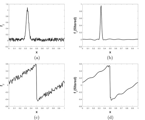
In order to illustrate the effect of wavelet regularization, we considered test function 1. To this test function, some noise δ is manually added to obtain $f_{\delta }$. The noisy function and corresponding filtered data using spectral graph wavelet are shown in Figure 15

Figure 15. Test function with noise and corresponding regularized data: (a) test function 1 with noise, (b) filtered function, (c) sawtooth function with discontinuity at x = 0.5 with noise and (d) filtered function.

5. Numerical results

Applying the change of variable $t\to T-t$ in problem (1(1) $\begin{array}{rl}{u}_t& =\nu \mathrm{△}u\mathrm{in}\Omega ,\\ u& =u_B\mathrm{on}\mathrm{\partial }D\times (0,T),\\ u& =u_F\mathrm{on}D\times \{T\}.\end{array}$(1) ), we retrieve the following formulation of the backward problem with $v(x,t)=u(x,T-t)$: (50) $\begin{array}{rl}{v}_t+\nu \mathrm{△}v& =0\mathrm{in}\Omega ,\\ v& =v_B\mathrm{on}\mathrm{\partial }D\times (0,T),\\ v& =v_F\mathrm{on}D\times \{0\}.\end{array}$(50)

Now, we apply the proposed numerical method on two different test problems in order to illustrate the efficiency and accuracy. All the computations are performed on MATLAB (9.0.0.341360 (R2016a)) software, on a 64 bit machine with processor Intel(R) Core(TM) i5-8250U CPU @1.80 GHz and 8 GB RAM. The operating system used is Windows 10 (version-1903).

Test problem 1: For test problem 1, we consider the BHCP given in (50(50) $\begin{array}{rl}{v}_t+\nu \mathrm{△}v& =0\mathrm{in}\Omega ,\\ v& =v_B\mathrm{on}\mathrm{\partial }D\times (0,T),\\ v& =v_F\mathrm{on}D\times \{0\}.\end{array}$(50) ) for $\mathrm{k}=1$, i.e. one-dimensional Laplacian operator with $\mathrm{△}v=v_{xx}$, boundary condition $v_B=0$ and bounded domain $\mathit{D}\in \mathit{[}\mathit{0}\mathit{,}\mathit{1}\mathit{]}$. To obtain $v_F=\mathrm{\Phi }(x)$, we first solve the forward heat conduction problem numerically using the initial condition $u(x,0)$ taken as test function 1. For all numerical examples, the scaling kernel $h(\lambda )$ and wavelet kernel $g(x)$ are choosen according to (8(8) $g(x)=\{\begin{array}{ll}{x}^2& \mathrm{for}0<x<1\\ -5+11x-6x^2+x^3& 1\le x\le 2\\ 4x^{-2}& \mathrm{for}x>2\end{array},$(8) ) and (9(9) $\mathsf{\text{h}}(\lambda )=\gamma {\mathrm{e}}^{-{\left(\frac{\lambda }{.6{\lambda }_{min}}\right)}^4},$(9) ) respectively.

To obtain noisy initial data ${\mathrm{\Phi }}^{\delta }(x)$ for our backward problem, we introduce some random noise η in $\mathrm{\Phi }(x)$, i.e. ${\mathrm{\Phi }}^{\delta }(x)=\mathrm{\Phi }(x)+\eta ,$ where $\eta =\delta \times rand(x)\times \Vert \mathrm{\Phi }{\Vert }_{\mathrm{\infty }}$,  rand(x) is the random vector obtained using MATLAB function ‘rand’ and δ is the noise parameter which is chosen according to the problem. For our numerical computation, we are using $\delta =5\times {10}^{-3}$. For comparing the numerical and exact solution, we use the following relative error: $e_2=\frac{\Vert v(.,t)-v_e(.,t){\Vert }_2}{\Vert v_e(.,t){\Vert }_2},$ where $v(.,t)$ and $v_e(.,t)$ stand for numerical and exact solution at time t for the problem considered.

For our numerical results, we have fixed J = 4 and the value of regularization parameter J, N and corresponding h is chosen as according to (4.2). The initial condition and corresponding adaptive grid are already shown in Figure 13(a). The regularized numerical solution for this problem and corresponding adaptive node arrangement using spectral graph wavelet method are shown in Figure 16 at different times. It is evident from the figure that the regularized solution becomes stable after wavelet filtering. The localized pattern of the solution is captured accurately and efficiently using the proposed method.

Figure 16. Evolution of the solution and dynamically adapted node arrangement for test problem 1 using $ϵ={10}^{-3},R=0.1,M=6$: (a) $T=0.1(N(ϵ)=176)$, (b) $T=0.4(N(ϵ)=248)$, (c) $T=0.8(N(ϵ)=301)$, (d) $T=1(N(ϵ)=377)$.

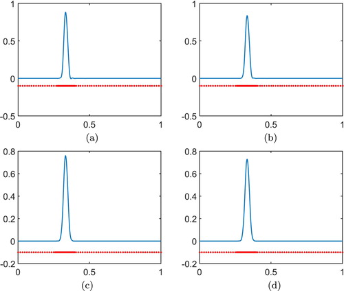
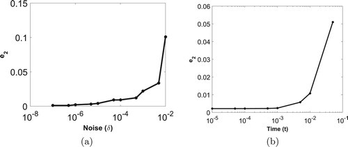
Figure 17(a) shows the plot of error between numerical and exact solution with noise δ for test problems 1. For this experiment, we fixed the time at $T={10}^{-2}$. The plot shows that error of regularized problem is less sensitive to noise. Moreover, it is observed that the growth rate of error suppresses after regularization. For example, at fixed $T={10}^{-2}$ and $\delta ={10}^{-2}$, error $e_2$ for original problem is $1.18\times {10}^{32}$ and for wavelet regularized solution is $2.95\times {10}^{-1}$. The plot in Figure 17(b) gives the relation of error with time for test problem 1 at fixed value of noise parameter which is $\delta ={10}^{-3}$. The figure shows that error increases with time after wavelet regularization but with less growth rate. The graph of error versus $N(ϵ)$ is given in Figure 18 which proves the convergence of the method. To compare our proposed method, we have solved test problem 1 with Fourier regularization method as given by Fu et al. in the paper [15]. We have compared both the results in terms of relative error and CPU time which is given in Table 1. From the table, it can be observed that the relative error using ASGWM and the method given in [15] are almost comparable. From the CPU time of both the methods, we can see that the proposed method is more efficient.

Figure 17. Plot of (a) error versus noise parameter δ with fixed $T={10}^{-2}$ and (b) error versus time T with fixed $\delta ={10}^{-3}$ for test problem 1.

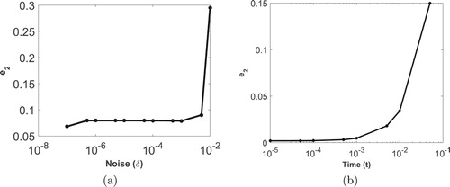
Figure 18. Plot of error versus $N(ϵ)$ for test problem 1.

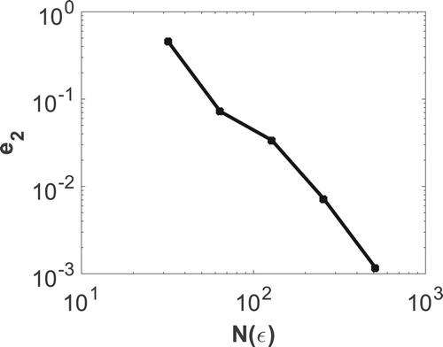
Table 1. Comparison of relative error for test problem 1 between Fu et al. [15] and ASGWM.

Time (T)	$e_2$ (Fu et al.)	$e_2$ (ASGWM)	CPU (Fu et al.)	CPU (ASGWM)
0.01	$6.24\times {10}^{-3}$	$8.47\times {10}^{-3}$	0.93	0.76
0.1	$1.21\times {10}^{-2}$	$0.82\times {10}^{-2}$	2.43	0.91
0.5	$7.53\times {10}^{-2}$	$7.07\times {10}^{-2}$	3.81	1.64
1	$2.60\times {10}^{-1}$	$3.19\times {10}^{-1}$	5.30	2.97

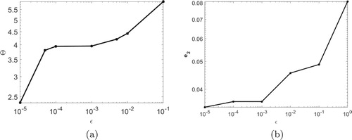
For efficiency of the proposed method, we have to calculate the efficiency coefficient Θ which is defined as $\mathrm{\Theta }=\frac{\mathrm{CPU}(ϵ=0)}{\mathrm{CPU}(ϵ)}$. Here, $\mathrm{CPU}(ϵ=0)$ is the CPU time taken by the finite difference method at $ϵ=0$ and $\mathrm{CPU}(ϵ)$ is the CPU time taken by ASGWM. The adaptive algorithm will be more efficient for larger efficiency coefficient. For the test problem 1, the plot of Θ versus ε is shown in Figure 19(a) and the plot of error versus ε is shown in Figure 19(b). From Figure 19(a), we can observe that the method is more efficient for large ε. But for large ε, as we can see from Figure 19(b) that error also increases as expected. Thus, for good accuracy and efficiency, we have to choose an optimal value of ε.

Figure 19. (a) Θ versus ε for test problem 1 at $t={10}^{-2}$. (b) $e_2$ versus ε for test problem 1.

Test problem 2: For test problem 2, we consider the problem (50(50) $\begin{array}{rl}{v}_t+\nu \mathrm{△}v& =0\mathrm{in}\Omega ,\\ v& =v_B\mathrm{on}\mathrm{\partial }D\times (0,T),\\ v& =v_F\mathrm{on}D\times \{0\}.\end{array}$(50) ) for $\mathrm{k}=2$, i.e. two-dimensional BHCP. For this problem, $\mathrm{△}v=v_{xx}+v_{yy}$ in bounded domain $\mathit{D}\in \mathit{[}\mathit{0}\mathit{,}\mathit{1}\mathit{]}\times \mathit{[}\mathit{0}\mathit{,}\mathit{1}\mathit{]}$ with boundary condition $v_B=0$. We solve the forward heat conduction problem numerically using the initial condition $u(x,0)$ which is same as test function 2 to obtain $v_F=\mathrm{\Phi }(x,y)$. 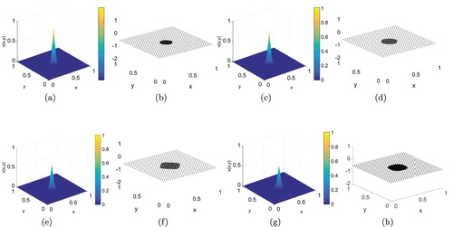In Figure 14, the initial condition for two-dimensional BHCP and corresponding adaptive grid are plotted. The stable regularized numerical solution and corresponding dynamically adaptive node arrangement using spectral graph wavelet method are shown in Figure 20 for different times. It can be easily demonstrated from the figure that proposed method is able to accurately and efficiently capture the emergence of localized pattern.

Figure 20. Evolution of the regularized numerical solution and corresponding dynamically adapted node arrangement for test problem 2 using $ϵ={10}^{-3},R=0.1,M=6$. (a) Solution for T = 0.1. (b) Adaptive node arrangement ($N(ϵ)=1258$). (c) Solution for T = 0.2. (d) Adaptive node arrangement ($N(ϵ)=2665$). (e) Solution for T = 0.4. (f) Adaptive node arrangement ($N(ϵ)=4382$). (g) Solution for T = 0.8. (h) Adaptive node arrangement ($N(ϵ)=4724$).

To see the performance of our proposed method, Table (2) is given which shows the values of $\mathrm{CPU}(ϵ)$ and corresponding Θ for different values of ε for test problem 2, $\mathrm{CPU}(ϵ=0)=3.1$. Relation between error in numerical and exact solution with noise for test problems 2 is shown in Figure 21(a) for fixed time $T={10}^{-2}$. In Figure 21(b), plot of error versus time at fixed value of noise parameter $\delta ={10}^{-3}$ is given for test problem 2. It is observed from numerical experiments and can be easily concluded from both the figures that the growth of error suppresses after regularization.

Table 2. The performance of ASGWM for test problem 2 with regularization.

ε	${10}^{-1}$	${10}^{-2}$	${10}^{-3}$	${10}^{-4}$	${10}^{-5}$
$\mathrm{CPU}(ϵ)$	0.51	0.68	0.73	0.891	1.21
Θ	6.078	4.55	4.24	3.479	2.561

Figure 21. Plot of (a) error versus noise parameter δ with fixed $T={10}^{-2}$ and (b) error versus time T with fixed $\delta ={10}^{-3}$ for test problem 2.

6. Conclusion and future work

In this paper, we have proposed a new regularization method based on spectral graph wavelet for stable solution of BHCP on graph. Fourth-order compact difference scheme with adaptive node technique is used to increase the efficiency of the proposed method. Fourier analysis shows that the fourth-order compact difference approximation has better resolution ability as compared to the standard fourth-order finite difference approximation. We have also provided the error estimate between the exact and wavelet regularized solution for BHCP. The efficiency and the convergence of the method is verified. To the best of our knowledge, till now, no one has proposed any regularization method to solved inverse problems on graph like structure. We want to point out here that the useful properties of spectral graph wavelet are for the first time exploited here for the solution of BHCP on graph.

In future, we will use spectral graph wavelet for the regularization of BHCP on a general/complex graph as well as for predicting shock waves. We will also try to extend the proposed method to solve some non-linear inverse problems. It will also be a good future research topic to solve some other complex inverse problems arises from real-life applications using this method.

Acknowledgments

The authors like to thanks the anonymous reviewers whose comments/suggestions helped improve and clarify this manuscript. The second author acknowledges the support provided by the Department of Science and Technology, India, under the grant number SERB/F/11946/2018-2019.

Disclosure statement

No potential conflict of interest was reported by the author(s).

Additional information

Funding

The second author acknowledges the support provided by the Department of Science and Technology, India, under the grant number SERB/F/11946/2018-2019.

References

- Isakov V. Inverse problems for partial differential equations. New York: Springer; 2006.
- Yin HM, Rundell W. A parabolic inverse problem with an unknown boundary condition. J Differ Equ. 1990;86:234–242. doi: 10.1016/0022-0396(90)90031-J
- Dehghan M. Determination of an unknown parameter in a semi-linear parabolic equation. Math Probl Eng. 2002;8:111–122. doi: 10.1080/10241230212906
- Mera NS, Elliott L, Ingham DB, et al. An iterative boundary element method for solving the one-dimensional backward heat conduction problem. Int J Heat Mass Transf. 2001;44:1937–1946. doi: 10.1016/S0017-9310(00)00235-0
- Liu CS. Group preserving scheme for backward heat conduction problems. Int J Heat Mass Transf. 2004;47:2567–2576. doi: 10.1016/j.ijheatmasstransfer.2003.12.019
- Beck JV, Blackwell B. Inverse heat conduction, Ill-posed problems. New York: Wiley Interscience; 1985.
- Engl HW, Hanke M, Neubauer A. Regularizaton of inverse problems. Dordrecht: Kluwer Academics; 1996.
- Hào DN. A mollification method for ill-posed problems. Numer Math. 1994;68:469–506. doi: 10.1007/s002110050073
- Han H, Ingham DB, Yuan Y. The boundary element method for the solution of the backward heat conduction equation. J Eng Des. 1994;516:292–299.
- Seidman TI. Optimal filtering for the backward heat equation. SIAM J Numer Anal. 1996;33:162–170. doi: 10.1137/0733010
- Lattès R, Lions JL. The method of quasi-reversibility. Applications to partial differential equations. Vol. 18. New York: American Elsevier Publishing Co., Inc.; 1969.
- Ames KA, Epperson JF. A kernel-based method for the approximate solution of backward parabolic problems. SIAM J Numer Anal. 1997;34:1357–1390. doi: 10.1137/S0036142994276785
- Kirkup SM, Wadsworth M. Solution of inverse diffusion problems by operator-splitting methods. Appl Math Model. 2002;26:1003–1018. doi: 10.1016/S0307-904X(02)00053-7
- Mera NS. The method of fundamental solutions for the backward heat conduction problem. Inverse Probl Sci Eng. 2005;13:65–78. doi: 10.1080/10682760410001710141
- Fu CL, Xiong XT, Qian Z. Fourier regularization for a backward heat equation. J Math Anal Appl. 2007;331:472–480. doi: 10.1016/j.jmaa.2006.08.040
- Xiong XT, Fu CL, Qian Z. Two numerical methods for solving a backward heat conduction problem. Appl Math Comput. 2006;179:370–377.
- Beck JV. Nonlinear estimation applied to the nonlinear inverse heat conduction problem. Int J Heat Mass Transf. 1970;13:703–716. doi: 10.1016/0017-9310(70)90044-X
- Lele SK. Compact finite difference schemes with spectral-like resolution. J Comput Phys. 1992;103:16–42. doi: 10.1016/0021-9991(92)90324-R
- Li J, Visbal MR. High order compact schemes for nonlinear dispersive waves. J Sci Comput. 2006;26:1–23. doi: 10.1007/s10915-004-4797-1
- Shukla RK, Tatineni M, Zhong X. Very high-order compact finite difference schemes on non-uniform grids for incompressible Navier–Stokes equations. J Comput Phys. 2007;224:1064–1094. doi: 10.1016/j.jcp.2006.11.007
- Patel KS, Mehra M. High order compact finite difference scheme for pricing asian option with moving boundary condition. Differ Equ Dyn Syst. 2017;27:39–56. doi: 10.1007/s12591-017-0372-8
- Kumar V. High-order compact finite-difference scheme for singularly-perturbed reaction-diffusion problems on a new mesh of Shishkin type. J Optim Theory Appl. 2009;143:123–147. doi: 10.1007/s10957-009-9547-y
- Pandit SK, Kalita JC, Dalal DC. A transient higher order compact scheme for incompressible viscous flows on geometries beyond rectangular equation on non-uniform grids. J Comput Phys. 2007;225:1100–1124. doi: 10.1016/j.jcp.2007.01.016
- Ahmed MO. An exploration of compact finite difference methods for the numerical solution of PDE [PhD dissertation]. Western Ontario London University; 1997.
- Mehra M. Wavelets theory and its applications. Singapore: Springer; 2018.
- Pourgholi R, Tavallaie N, Foadian S. Applications of Haar basis method for solving some ill-posed inverse problems. J Math Chem. 2012;50:2317–2337. doi: 10.1007/s10910-012-0036-4
- Lepik Ü. Numerical solution of evolution equations by the Haar wavelet method. Appl Math Comput. 2007;185:695–704.
- Razzaghi M. Legendre wavelets method for the solution of nonlinear problems in the calculus of variations. Math Comput Model. 2001;34:45–54. doi: 10.1016/S0895-7177(01)00048-6
- Babolian E, Fattahzadeh F. Numerical solution of differential equations by using Chebyshev wavelet operational matrix of integration. Appl Math Comput. 2007;188:417–426.
- Oruç Ö. A computational method based on Hermite wavelets for two-dimensional Sobolev and regularized long wave equations in fluids. Numer Methods Partial Differ Equ. 2018;34:1693–1715. doi: 10.1002/num.22232
- Adibi H, Assari P. Using CAS wavelets for numerical solution of Volterra integral equations of the second kind. Dyn Continuous Discrete Impulsive Syst Ser A. 2009;16:673–685.
- Adibi H, Assari P. Chebyshev wavelet method for numerical solution of Fredholm integral equations of the first kind. Math Prob Eng. 2010;2010:1–17. doi: 10.1155/2010/138408
- Adibi H, Assari P. On the numerical solution of weakly singular Fredholm integral equations of the second kind using Legendre wavelets. J Vib Control. 2011;17:689–698. doi: 10.1177/1077546310366865
- Assari P, Dehghan M. Application of dual-Chebyshev wavelets for the numerical solution of boundary integral equations with logarithmic singular kernels. Eng Comput. 2019;35:175–190. doi: 10.1007/s00366-018-0591-9
- Eldén L, Berntsson F, Regińska T. Wavelet and Fourier methods for solving the sideways heat equation. SIAM J Sci Comput. 2000;21:2187–2205. doi: 10.1137/S1064827597331394
- Qiu CY, Fu CL. Wavelets and regularization of the Cauchy problem for the Laplace equation. J Math Anal Appl. 2008;338:1440–1447. doi: 10.1016/j.jmaa.2007.06.035
- Regińska T, Wakulicz A. Wavelet moment method for the Cauchy problem for the Helmholtz equation. J Comput Appl Math. 2009;223:218–229. doi: 10.1016/j.cam.2008.01.005
- Wang JR. Shannon wavelet regularization methods for a backward heat equation. J Comput Appl Math. 2011;235:3079–3085. doi: 10.1016/j.cam.2011.01.001
- Hammond DK, Vandergheynst P, Gribonval R. Wavelets on graphs via spectral graph theory. Appl Comput Harmon Anal. 2011;30:129–150. doi: 10.1016/j.acha.2010.04.005
- Zhang L, Ouyang J, Wang X, et al. Variational multiscale element-free Galerkin's method for 2D Burger's equation. J Comput Phys. 2010;229:7147–7161. doi: 10.1016/j.jcp.2010.06.004
- Jameson L. A wavelet-optimized, very high order adaptive grid and order numerical method. SIAM J Sci Comput. 1998;19:1980–2013. doi: 10.1137/S1064827596301534
- Goyal K, Mehra M. A fast adaptive diffusion wavelet method for Burgers equations. Comput Math Appl. 2014;4:568–577. doi: 10.1016/j.camwa.2014.06.007
- Goyal K, Mehra M. An adaptive meshfree spectral graph wavelet method for partial differential equations. Appl Numer Math. 2017;113:168–185. doi: 10.1016/j.apnum.2016.11.011
- Shukla A, Mehra M, Leugering G. A fast adaptive spectral graph wavelet method for the viscous Burgers'equation on a star-shaped connected graph. Math Method Appl Sci. 2019: 1–20. doi: 10.1002/mma.5907
- Mehra M, Patel KS. Algorithm 986: a suite of compact finite difference schemes. ACM Trans Math Softw. 2017;44:1–31. doi: 10.1145/3119905
- Daripa P. Some useful filtering techniques for illposed problems. J Comput Appl Math. 1998;2:161–171. doi: 10.1016/S0377-0427(98)00186-1