Chebyshev pseudospectral method in the reconstruction of orthotropic conductivity

Abstract

In this paper, we present a method to reconstruct the spatially varying conductivity tensor in isotropic and orthotropic materials, involved in a two-dimensional transient anisotropic model with Robin boundary conditions. For the reconstruction, the partial differential equation is solved by a semi-discrete method that combines a pseudospectral collocation method for spatial variables and Crank–Nicolson for time. The conductivity tensor is reconstructed through a non-linear least-squares problem solved by Levenberg–Marquardt method (LMM), along with Morozov's discrepancy principle as stopping rule to cope with noise in the data. Unlike classic LMM implementations that mitigate poor conditioning in calculating iterates using nonsingular diagonal scaling matrices, in this paper, singular regularization matrices are used. The impact of such a modification is illustrated with numerical experiments using discrete differential operators as scaling matrices. Numerical results show that accurate conductivity values can be obtained using a fairly small number of discretization points at a very low computational cost.

Keywords:

• Orthotropic conductivity reconstruction
• Chebyshev pseudospectral method
• Levenberg–Marquardt method
• Morozov's discrepancy principle
• inverse problem

2010 Mathematics Subject Classifications:

• 65M70
• 65M32

1. Introduction

Materials whose physical properties, such as elasticity moduli, Poisson coefficients, heat conductivity, etc., vary depending on spatial orientation of the physical body are referred to as anisotropic, while those materials that do not change with spatial orientation are referred to as isotropic [1]. Orthotropic material is a type of the anisotropic material whose characteristics remain unchanged along its planes of elastic symmetry. In nature, there are many materials that can be considered anisotropic such as crystal, woods, geological sediments and biological tissues. With the advent of new technologies, new anisotropic materials have been manufactured by industrial engineering, making it necessary to know their driving properties. These properties can be roughly defined by the difference in physical material or mechanical attributes when measured along different axes, such as absorbance, refraction, conductivity, tensile strength, etc.

In this paper, we study anisotropy in a two-dimensional transient conduction problem, with spatially varying conductivity tensor, aiming at a practical method for conductivity estimation based on experimental transient data.

Consider a two-dimensional anisotropic transport problem in the finite domain $\mathrm{\Gamma }\times (0,\overline{t}]$, $\overline{t}>0$, with $\mathrm{\Gamma }=(0,1)\times (0,1)\subseteq {\mathbb{R}}^2$, where $\mathbb{R}$ denotes the set of real numbers, described by the partial differential equation (1) $C(x,y)\frac{\mathrm{\partial }T}{\mathrm{\partial }t}(x,y,t)=\mathrm{\nabla }\cdot [K(x,y)\mathrm{\nabla }T(x,y,t)]+g(x,y,t)\mathrm{in}\mathrm{region}\mathrm{\Gamma }\times (0,\overline{t}],$(1) constrained to boundary conditions (2) $\begin{array}{rl}-(K\mathrm{\nabla }T)\cdot \mathbf{n}=f_1(y,t),& \mathrm{on}x=0,y\in (0,1),t\in (0,\overline{t}],\end{array}$(2) (3) $\begin{array}{rl}-(K\mathrm{\nabla }T)\cdot \mathbf{n}+h_2(y)T(1,y,t)=f_2(y,t),& \mathrm{on}x=1,y\in (0,1),t\in (0,\overline{t}],\end{array}$(3) (4) $\begin{array}{rl}-(K\mathrm{\nabla }T)\cdot \mathbf{n}=f_3(x,t),& \mathrm{on}y=0,x\in (0,1),t\in (0,\overline{t}],\end{array}$(4) (5) $\begin{array}{rl}-(K\mathrm{\nabla }T)\cdot \mathbf{n}+h_4(x)T(x,1,t)=f_4(x,t),& \mathrm{on}y=1,x\in (0,1),t\in (0,\overline{t}],\end{array}$(5) and initial condition (6) $T(x,y,0)=T_0(x,y)\mathrm{in}\mathrm{region}\mathrm{\Gamma }.$(6) In this model, $T(x,y,t)$ stands for temperature, C>0 is the heat capacity, K is the conductivity matrix, (7) $K(x,y)=\left[\begin{array}{cc}{k}_{11}(x,y)& k_{12}(x,y)\\ k_{21}(x,y)& k_{22}(x,y)\end{array}\right]$(7) and g is a source term. In addition, $h_i$, i = 2, 4, are heat transfer functions, $f_i$, $i=1,\dots ,4$, are heat flux functions, and $\mathbf{n}=[{\mathbf{n}}_x{\mathbf{n}}_y{]}^{\mathrm{T}}$ is the outward unit normal vector to the boundary of Γ. Here and elsewhere superscript $\mathrm{T}$ stands for transpose of a vector or a matrix. For future development and to be clear with the notation, observe that $-(K\mathrm{\nabla }T)\cdot \mathbf{n}=-(k_{11}\frac{\mathrm{\partial }T}{\mathrm{\partial }x}+k_{12}\frac{\mathrm{\partial }T}{\mathrm{\partial }y}){\mathbf{n}}_x-(k_{21}\frac{\mathrm{\partial }T}{\mathrm{\partial }x}+k_{22}\frac{\mathrm{\partial }T}{\mathrm{\partial }y}){\mathbf{n}}_y.$ The conductivity K is assumed continuous and positive definite matrix, which means $k_{11}>0$ and $k_{11}{k}_{22}-k_{12}{k}_{21}>0$. To classify the problem, K is said to be isotropic ($k_{11}=k_{22},k_{12}=k_{21}=0$), orthotropic ($k_{11}\ne k_{22},k_{12}=k_{21}=0$) or anisotropic ($k_{11}\ne k_{22},k_{12}\ne 0$, $k_{21}\ne 0$). We note in passing that model (1(1) $C(x,y)\frac{\mathrm{\partial }T}{\mathrm{\partial }t}(x,y,t)=\mathrm{\nabla }\cdot [K(x,y)\mathrm{\nabla }T(x,y,t)]+g(x,y,t)\mathrm{in}\mathrm{region}\mathrm{\Gamma }\times (0,\overline{t}],$(1) )–(6(6) $T(x,y,0)=T_0(x,y)\mathrm{in}\mathrm{region}\mathrm{\Gamma }.$(6) ) is also encountered in other applications areas in which K does not necessarily stand for thermal conductivity and where $T(x,y,t)$ describes transient data of other nature as, e.g. electrostatic potential [2–4]. Irrespective of the application under consideration, several problems associated with model (1(1) $C(x,y)\frac{\mathrm{\partial }T}{\mathrm{\partial }t}(x,y,t)=\mathrm{\nabla }\cdot [K(x,y)\mathrm{\nabla }T(x,y,t)]+g(x,y,t)\mathrm{in}\mathrm{region}\mathrm{\Gamma }\times (0,\overline{t}],$(1) )–(6(6) $T(x,y,0)=T_0(x,y)\mathrm{in}\mathrm{region}\mathrm{\Gamma }.$(6) ) are found in literature and we are concerned with two of them. The first one, referred to as forward or direct problem, devoted to determine the function $T(x,y,t)$ satisfying (1(1) $C(x,y)\frac{\mathrm{\partial }T}{\mathrm{\partial }t}(x,y,t)=\mathrm{\nabla }\cdot [K(x,y)\mathrm{\nabla }T(x,y,t)]+g(x,y,t)\mathrm{in}\mathrm{region}\mathrm{\Gamma }\times (0,\overline{t}],$(1) )–(6(6) $T(x,y,0)=T_0(x,y)\mathrm{in}\mathrm{region}\mathrm{\Gamma }.$(6) ) where the remaining parameters are regarded as input data, and the second one referred to as an inverse problem, where the conductivity K is regarded as unknown and has to be estimated from measured temperature data. In this regard, it is known that, while the forward problem is governed by a linear elliptic well-posed operator, this is not the case with the inverse problem, which is non-linear and is ill-posed [5, Chapter 9]. In fact, it is not obvious whether the conductivity K is (uniquely) determined by the data T. However, it is known that the uniqueness of the solution is only valid in some special cases [5,6]. For example, in the isotropic case, we quote the recovery of a discontinuous conductivity in a multidimensional problem with null source and homogeneous boundary conditions [7], the identification problem of aquifer parameters [8], and a 1D identification problem under certain Hölder smoothness conditions [9]; for the orthotropic case, we quote the recovery of thermal conductivity from heat flux measurements [10], whereas for the anisotropic case, we highlight the conductivity reconstruction problem on the homogeneous steady-state case under the constraint that the conductor is known up to an unknown multiple scalar [11]. Anyway, even if the reconstruction problem allows for a (unique) solution, as the problem is ill-posed, small data errors can result in major disturbances in the solution, i.e. the solution does not depend continuously on the data.

Many studies to identify anisotropic conductivity from experimental data have been developed and reported in the literature [12–14]. However, the limited availability of observational measures as well as the indirect nature of the estimation itself makes the problem solution difficult and thus more effective inverse solution techniques should be utilized. It is noteworthy that, in particular for the conduction problem addressed in this paper, Equations  (1(1) $C(x,y)\frac{\mathrm{\partial }T}{\mathrm{\partial }t}(x,y,t)=\mathrm{\nabla }\cdot [K(x,y)\mathrm{\nabla }T(x,y,t)]+g(x,y,t)\mathrm{in}\mathrm{region}\mathrm{\Gamma }\times (0,\overline{t}],$(1) )–(6(6) $T(x,y,0)=T_0(x,y)\mathrm{in}\mathrm{region}\mathrm{\Gamma }.$(6) ), closed form solutions exist only for the orthotropic conductivity case, which does not happen for the anisotropic case [15]. On the other hand, the inverse problem of reconstructing an anisotropic conductivity based on the steady-state assumption, in general, is not unique, even knowing the complete heat/current flux at the boundary [11]. A similar observation holds true for the isotropic case, where conductivity is uniquely identified when the full Dirichlet-to-Neumann boundary map is known [16], which is not always available in practice. To overcome this difficulty, other schemes were hence developed, including more information on the problem such as evaluations of temperature/potential inside the solution domain. As an example, Mera et al. [17] applied the boundary element method (BEM) to solve the Cauchy steady-state heat conduction problem in an anisotropic medium. Other BEM-like techniques may be found in [18,19]. Recently, in connection with a time-dependent model, a finite difference method (FDM) has been employed together with a regularized non-linear minimization process to determine the orthotropic inhomogeneous tensor [20]. In this case, numeric experiments were accomplished using the MATLAB lsqnonlin toolbox routine. In a similar flavour, a method for reconstructing orthotropic thermal conductivity based on the combination of FDM based on an alternating-direction-implicit scheme for solving the direct problem and the conjugate gradient method (CGM) as optimization tool, has been recently reported in [21]. The novelty here is that the optimization problem is formulated in the $L_2$ infinite-dimensional environment, which is interesting, but can be expensive due to the calculation of the involved $L_2$-norm.

As mentioned above, mathematically equivalent applications for the conduction problem include reconstruction of electrical conductivity. For instance, in medical imaging applications, the numerical reconstructions of anisotropic conductivity arises in electrical impedance tomography [2–4,22]. Several techniques for computing anisotropic conductivity in this context have been used. In particular, in thermal tomography [23], where the coefficient K is characterized by a finite number of parameters in a high-dimensional subset of ${\mathbb{R}}^p$ referred to as parameter domain, the direct problem is solved by coupling the finite element methods (FEM) in the spatial domain and a semi-implicit Euler method in the time interval. On its turn, the inverse problem is formulated as a non-linear least squares problem coupled with Tikhonov regularization. In contrast, in [24], the parameter identification problem is modelled as a variational problem over stochastic Sobolev spaces, where a spectral approximation of the observation field is used to estimate the solution problem using a finite noisy model. In resume, most of these techniques approach the partial differential equation given by (1(1) $C(x,y)\frac{\mathrm{\partial }T}{\mathrm{\partial }t}(x,y,t)=\mathrm{\nabla }\cdot [K(x,y)\mathrm{\nabla }T(x,y,t)]+g(x,y,t)\mathrm{in}\mathrm{region}\mathrm{\Gamma }\times (0,\overline{t}],$(1) ), with Neumann, Dirichlet or mixed boundary conditions, by using one or more numerical methods, then an objective function is formulated and an optimization technique is chosen to find an optimal parameter.

The Chebyshev pseudospectral method (CPM), also referred to as orthogonal collocation, is a method for computing approximate solutions of ordinary or partial differential equations. It differs from other methods such as finite difference methods in that the solution is represented as a continuous or piecewise continuous function [25]. Further, compared to other methods such as BEM or FEM, CPM is known to produce highly accurate solutions at lower computation cost, see, e.g. [26–31]. The purpose of this paper is to offer an alternative method to reconstruct the orthotropic conductivity tensor, which is simple to implement and generalize to the anisotropic case, and relatively inexpensive when compared to existing ones. The main idea behind the method is to combine an efficient solver for the direct problem and the acknowledged value of the Levenberg–Marquardt method in solving non-linear last squares methods. Specifically, the solver involves a spatial discretization of the conduction problem (1(1) $C(x,y)\frac{\mathrm{\partial }T}{\mathrm{\partial }t}(x,y,t)=\mathrm{\nabla }\cdot [K(x,y)\mathrm{\nabla }T(x,y,t)]+g(x,y,t)\mathrm{in}\mathrm{region}\mathrm{\Gamma }\times (0,\overline{t}],$(1) )–(6(6) $T(x,y,0)=T_0(x,y)\mathrm{in}\mathrm{region}\mathrm{\Gamma }.$(6) ), through Chebyshev pseudospectral method and the solution of the resulting semi-discrete model using the trapezoidal rule in time. The inverse conduction problem is solved through Levenberg–Marquardt method based on a version of Yamashita and Fukushima [32], along with Morozov's discrepancy principle [33] as stopping rule to cope with noisy data. In this respect, as opposed to classic LMM implementations that mitigate poor conditioning in calculating iterates using nonsingular diagonal scaling matrices, in this paper singular regularization matrices are used. This marks a significant difference from the version of LMM implemented in lsqnonlin used in [20]. In addition, since the chosen regularization matrices correspond to discrete versions of differential operators, they produce, without additional cost, a smoothing effect in the computed solution similar to that produced by the Sobolev gradient used in [21] (at the expense of additional work).

This paper is organized as follows. In Section 2, we consider the conduction model (1(1) $C(x,y)\frac{\mathrm{\partial }T}{\mathrm{\partial }t}(x,y,t)=\mathrm{\nabla }\cdot [K(x,y)\mathrm{\nabla }T(x,y,t)]+g(x,y,t)\mathrm{in}\mathrm{region}\mathrm{\Gamma }\times (0,\overline{t}],$(1) )–(6(6) $T(x,y,0)=T_0(x,y)\mathrm{in}\mathrm{region}\mathrm{\Gamma }.$(6) ) in the isotropic case, with the conductivity as input data, and derive a semi-discrete model for the forward problem using CPM in order to compute function values T (temperature or electrostatic potential). Then, in Section 3, we describe and analyse a strategy to solve the inverse problem of finding conductivity values based on measured values of T at a few time steps, including in particular, a method for computing Jacobians as well as a precise description of LMM with singular regularization matrices instead of scaling diagonal matrices. Numerical results are also included. Section 4 follows the same organization as Section 3 but now in connection with the orthotropic scenario. We finish the paper with conclusions and references.

2. Chebyshev pseudospectral method for forward problem – isotropic case

In this section, we will describe how to solve (1(1) $C(x,y)\frac{\mathrm{\partial }T}{\mathrm{\partial }t}(x,y,t)=\mathrm{\nabla }\cdot [K(x,y)\mathrm{\nabla }T(x,y,t)]+g(x,y,t)\mathrm{in}\mathrm{region}\mathrm{\Gamma }\times (0,\overline{t}],$(1) )–(6(6) $T(x,y,0)=T_0(x,y)\mathrm{in}\mathrm{region}\mathrm{\Gamma }.$(6) ) with the Chebyshev pseudospectral method. This method has become popular in solving ordinary or partial differential equations (PDEs) due to its high accuracy and lower computational cost compared with finite difference or finite element-based methods and has been successfully applied in solving forward and inverse heat conduction problems, see, e.g. [27–29]. The construction of highly accurate solutions for PDEs lies on the fact that spatial derivatives can be approximated to high precision by means of the Chebyshev differentiation matrix.

Roughly speaking, pseudospectral methods construct approximate solutions in a space of algebraic polynomials of lower degree so that the differential equation being solved is satisfied in a specified number of points referred to as collocation points. For linear stationary and unidimensional problems on a bounded interval, for instance, if the collocation points are denoted by $x_j$, $j=0,\dots ,n$, and if the approximate solution is denoted by $u_n$ and expressed as (8) $u_n(x)=\sum _{k=0}^n{\alpha }_k{\ell }_k(x),$(8) where ${\alpha }_k\doteq u_n(x_k),k=0,\dots ,n$, and ${\ell }_k(x)$ denotes the related Lagrange polynomial, then the coefficients ${\alpha }_j$ become the unknowns of a linear system obtained by discretizing the differential equation in such a way that derivatives of the exact solution are estimated at the collocation points by differentiating (8(8) $u_n(x)=\sum _{k=0}^n{\alpha }_k{\ell }_k(x),$(8) ) and evaluating the result at $x_j$. As a matter of fact, note that derivative values $u_n^{\prime }(x_j)$, $u_n^{\prime }(x_j)=\sum _{k=0}^n{\alpha }_k{\ell }_k^{\prime }(x_j),j=0,\dots n,$ can be expressed in matrix form as (9) ${\mathsf{\text{u}}}_n^{(1)}=D{\mathsf{\text{u}}}_n,$(9) with ${\mathsf{\text{u}}}_n^{(1)}=[u_n^{\prime }(x_0),\dots ,u_n^{\prime }(x_n){]}^{\mathrm{T}},{\mathsf{\text{u}}}_n=[u_n(x_0),\dots ,u_n(x_n){]}^{\mathrm{T}},$ where D denotes the $(n+1)\times (n+1)$ differentiation matrix whose entries are (10) $D_{j,k}={\ell }_k^{\prime }(x_j),j=0,\dots ,n,k=0,\dots ,n.$(10) A consequence of (9(9) ${\mathsf{\text{u}}}_n^{(1)}=D{\mathsf{\text{u}}}_n,$(9) ) is that if $u_n(x)$ interpolates $u(x)$ at the collocation points, derivative values $u^{\prime }(x_j)$ can be approximated as $u^{\prime }(x_j)\approx u_n^{\prime }(x_j)$ [30], or in vector form, with abuse of notation, as (11) $\left[\begin{array}{c}{u}^{\prime }(x_0)\\ ⋮\\ u^{\prime }(x_n)\end{array}\right]\approx {\mathsf{\text{u}}}_n^{(1)}=D\left[\begin{array}{c}u(x_0)\\ ⋮\\ u(x_n)\end{array}\right].$(11) The Chebyshev pseudospectral method takes as collocation points the Chebyshev–Gauss–Lobatto points, (12) $x_j=\cos \left(\frac{\pi j}{n}\right),j=0,\dots ,n,$(12) and for this case, explicit formulas for $D_{j,k}$ can be found in several references, see e.g. [30]. Without getting into any details, we note that for the Chebyshev differentiation matrix the following $L_2$ discrete estimate for $u^{\prime }$ at the collocation points is known to hold [34, Chapter 9, estimate 9.5.22] (13) $\Vert u^{\prime }-u_n^{\prime }\Vert =\mathcal{O}(n^{2-m})$(13) where m denotes the regularity (smoothness) of u. This result implies that (11(11) $\left[\begin{array}{c}{u}^{\prime }(x_0)\\ ⋮\\ u^{\prime }(x_n)\end{array}\right]\approx {\mathsf{\text{u}}}_n^{(1)}=D\left[\begin{array}{c}u(x_0)\\ ⋮\\ u(x_n)\end{array}\right].$(11) ) can lead to exponential order of convergence as far as u is sufficiently smooth. In words, the smoother the function u, the smaller the approximation error. We will end this very short explanation on pseudospectral methods by noting that multidimensional problems are treated similarly as above. For 2D cases for instance, if for the sake of simplicity we use the same number of collocation points, n + 1, in the x and y directions, then the Chebyshev pseudospectral method looks as approximate solution for a polynomial $u_n(x,y)$, $u_n(x,y)=\sum _{j=0}^n\sum _{k=0}^n{u}_n(x_j,y_k){\ell }_j(x){\ell }_k(y),$ where $u_n(x_j,y_j)$ are unknowns to be determined by requiring that the given equation (and boundary condition) is satisfied at the grid points $(x_j,y_k)$. For PDEs with time and space variables, on the other hand, the construction of the approximate solution is as above but with the sole difference that the problem is now transformed into a time-dependent system of ordinary differential equations for which several methods exist.

Returning to the problem we are concerned with, we will first focus on the isotropic case to describe more clearly how CPM works. As mentioned above this case means $k_{11}=k_{22}=:k$ and $k_{12}=k_{21}=0$, which simplifies the numerical analysis. Therefore we can rewrite (1(1) $C(x,y)\frac{\mathrm{\partial }T}{\mathrm{\partial }t}(x,y,t)=\mathrm{\nabla }\cdot [K(x,y)\mathrm{\nabla }T(x,y,t)]+g(x,y,t)\mathrm{in}\mathrm{region}\mathrm{\Gamma }\times (0,\overline{t}],$(1) ) as (14) $C(x,y)\frac{\mathrm{\partial }T}{\mathrm{\partial }t}(x,y,t)={\displaystyle \frac{\mathrm{\partial }}{\mathrm{\partial }x}}(k(x,y){\displaystyle \frac{\mathrm{\partial }T}{\mathrm{\partial }x}}(x,y,t))+{\displaystyle \frac{\mathrm{\partial }}{\mathrm{\partial }y}}(k(x,y){\displaystyle \frac{\mathrm{\partial }T}{\mathrm{\partial }y}}(x,y,t))+g(x,y,t).$(14) For simplicity, we shall consider a mesh consisting of $(n+1)\times (n+1)$ points on the reference domain Γ based on $(n+1)$ Chebyshev–Gauss–Lobatto points in the horizontal and vertical directions, (15) $x_i=\frac{1}{2}[1-\cos \left(\frac{i\pi }{n}\right)],i=0,\dots ,n,y_j=\frac{1}{2}[1-\cos \left(\frac{j\pi }{n}\right)],j=0,\dots ,n,$(15) and assume that grid points are numbered in lexicographic ordering. Assume also that the Chebyshev differentiation matrix is expressed in row-wise (resp. column-wise) form, (16) $D=\left[\begin{array}{c}{r}_0^{\mathrm{T}}\\ ⋮\\ r_n^{\mathrm{T}}\end{array}\right]=[d_0,\dots ,d_n],r_i,d_i\in {\mathbb{R}}^{n+1},i=0,\dots ,n.$(16) The next step is to approximate spatial derivatives in (14(14) $C(x,y)\frac{\mathrm{\partial }T}{\mathrm{\partial }t}(x,y,t)={\displaystyle \frac{\mathrm{\partial }}{\mathrm{\partial }x}}(k(x,y){\displaystyle \frac{\mathrm{\partial }T}{\mathrm{\partial }x}}(x,y,t))+{\displaystyle \frac{\mathrm{\partial }}{\mathrm{\partial }y}}(k(x,y){\displaystyle \frac{\mathrm{\partial }T}{\mathrm{\partial }y}}(x,y,t))+g(x,y,t).$(14) ) by using matrix D. In fact, along the horizontal direction, we have (17) ${\displaystyle \frac{\mathrm{\partial }}{\mathrm{\partial }x}}(k(x_i,y_j){\displaystyle \frac{\mathrm{\partial }T}{\mathrm{\partial }x}}(x_i,y_j,t))\approx e_{i+1}^{\mathrm{T}}D{\mathbf{K}}_j^x{\dot{\mathbf{T}}}_j,i=0,\dots ,n,j=0,1,\dots ,n,$(17) where $e_i$, denotes the i-th canonical vector in ${\mathbb{R}}^{n+1}$, ${\mathbf{K}}_j^x$ is the diagonal matrix (18) ${\mathbf{K}}_j^x=\mathrm{diag}(k(x_0,y_j),k(x_1,y_j),\dots ,k(x_n,y_j)),j=0,1,\dots ,n,$(18) and ${\dot{\mathbf{T}}}_j$ is the column vector (19) ${\dot{\mathbf{T}}}_j={[{\displaystyle \frac{\mathrm{\partial }T}{\mathrm{\partial }x}}(x_0,y_j,t),{\displaystyle \frac{\mathrm{\partial }T}{\mathrm{\partial }x}}(x_1,y_j,t),\dots ,{\displaystyle \frac{\mathrm{\partial }T}{\mathrm{\partial }x}}(x_n,y_j,t)]}^{\mathrm{T}},j=0,1,\dots ,n.$(19) Clearly, provided the functions k and T are sufficiently regular, the order of approximation of (17(17) ${\displaystyle \frac{\mathrm{\partial }}{\mathrm{\partial }x}}(k(x_i,y_j){\displaystyle \frac{\mathrm{\partial }T}{\mathrm{\partial }x}}(x_i,y_j,t))\approx e_{i+1}^{\mathrm{T}}D{\mathbf{K}}_j^x{\dot{\mathbf{T}}}_j,i=0,\dots ,n,j=0,1,\dots ,n,$(17) ) is analogous to that given in (13(13) $\Vert u^{\prime }-u_n^{\prime }\Vert =\mathcal{O}(n^{2-m})$(13) ). Now let ${\mathbf{T}}_j^x$ be defined by (20) ${\mathbf{T}}_j^x=\left[\begin{array}{c}{\displaystyle \frac{\mathrm{\partial }}{\mathrm{\partial }x}}(k(x_0,y_j){\displaystyle \frac{\mathrm{\partial }T}{\mathrm{\partial }x}}(x_0,y_j,t))\\ ⋮\\ {\displaystyle \frac{\mathrm{\partial }}{\mathrm{\partial }x}}(k(x_n,y_j){\displaystyle \frac{\mathrm{\partial }T}{\mathrm{\partial }x}}(x_n,y_j,t))\end{array}\right],j=0,1,\dots ,n.$(20) With this notation, observe that the approximation (17(17) ${\displaystyle \frac{\mathrm{\partial }}{\mathrm{\partial }x}}(k(x_i,y_j){\displaystyle \frac{\mathrm{\partial }T}{\mathrm{\partial }x}}(x_i,y_j,t))\approx e_{i+1}^{\mathrm{T}}D{\mathbf{K}}_j^x{\dot{\mathbf{T}}}_j,i=0,\dots ,n,j=0,1,\dots ,n,$(17) ) can be expressed in vector form as (21) ${\mathbf{T}}_j^x\approx D{\mathbf{K}}_j^x{\dot{\mathbf{T}}}_j=\sum _{i=0}^n{d}_{i}k(x_i,y_j){\displaystyle \frac{\mathrm{\partial }T}{\mathrm{\partial }x}}(x_i,y_j,t),$(21) and that, since the boundary conditions (2(2) $\begin{array}{rl}-(K\mathrm{\nabla }T)\cdot \mathbf{n}=f_1(y,t),& \mathrm{on}x=0,y\in (0,1),t\in (0,\overline{t}],\end{array}$(2) )–(3(3) $\begin{array}{rl}-(K\mathrm{\nabla }T)\cdot \mathbf{n}+h_2(y)T(1,y,t)=f_2(y,t),& \mathrm{on}x=1,y\in (0,1),t\in (0,\overline{t}],\end{array}$(3) ) and (16(16) $D=\left[\begin{array}{c}{r}_0^{\mathrm{T}}\\ ⋮\\ r_n^{\mathrm{T}}\end{array}\right]=[d_0,\dots ,d_n],r_i,d_i\in {\mathbb{R}}^{n+1},i=0,\dots ,n.$(16) ) imply (22) $\begin{array}{rl}{\displaystyle \sum _{i=0}^n{d}_{i}k(x_i,y_j){\displaystyle \frac{\mathrm{\partial }T}{\mathrm{\partial }x}}(x_i,y_j,t)}& =d_0{f}_1(y_j,t)+{\displaystyle \sum _{i=1}^{n-1}{d}_{i}k(x_i,y_j){\displaystyle \frac{\mathrm{\partial }T}{\mathrm{\partial }x}}(x_i,y_j,t)}\\ & +d_n{h}_2(y_j)T(x_n,y_j,t)-d_n{f}_2(y_j,t)\\ & =[D_1{\check{\mathbf{K}}}_j{D}_2+h_2(y_j)d_n{e}_{n+1}^{\mathrm{T}}]{\mathbf{T}}_j(t)\\ & +d_0{f}_1(y_j,t)-d_n{f}_2(y_j,t),\end{array}$(22) where (23) $\begin{array}{rl}{\mathbf{T}}_j(t)& =[T(x_0,y_j,t),T(x_1,y_j,t),\dots ,T(x_n,y_j,t){]}^{\mathrm{T}},\end{array}$(23) $\begin{array}{rl}{D}_1& =[d_1,\dots ,d_{n-1}],D_2=\left[\begin{array}{c}{r}_1^{\mathrm{T}}\\ ⋮\\ r_{n-1}^{\mathrm{T}}\end{array}\right],{\check{\mathbf{K}}}_j=\mathrm{diag}(k(x_1,y_j),\dots ,k(x_{n-1},y_j)),\end{array}$ we conclude that (24) ${\mathbf{T}}_j^x\approx [D_1{\check{\mathbf{K}}}_j{D}_2+h_2(y_j)d_n{e}_{n+1}^{\mathrm{T}}]{\mathbf{T}}_j+d_0{f}_1(y_j,t)-d_n{f}_2(y_j,t).$(24) Before proceeding, note that although ${\mathbf{T}}_j$ is a vector function in ${\mathbb{R}}^{n+1}$ that depends on time, to simplify the notation, ${\mathbf{T}}_j(t)$ will be denoted by ${\mathbf{T}}_j$. With this convention and based on (24(24) ${\mathbf{T}}_j^x\approx [D_1{\check{\mathbf{K}}}_j{D}_2+h_2(y_j)d_n{e}_{n+1}^{\mathrm{T}}]{\mathbf{T}}_j+d_0{f}_1(y_j,t)-d_n{f}_2(y_j,t).$(24) ), discretization of ${\displaystyle \frac{\mathrm{\partial }}{\mathrm{\partial }x}}(k(x,y){\displaystyle \frac{\mathrm{\partial }T}{\mathrm{\partial }x}}(x,y,t))$ along all grid points with $T(x_i,y_j,t)$ enumerated in lexicographic order leads to (25) $\left[\begin{array}{c}{\mathbf{T}}_0^x\\ {\mathbf{T}}_1^x\\ ⋮\\ {\mathbf{T}}_n^x\end{array}\right]\approx \left(\begin{array}{cccc}{\mathbf{F}}_0& & & \\ & {\mathbf{F}}_1& & \\ & & \ddots & \\ & & & {\mathbf{F}}_n\end{array}\right)\left[\begin{array}{c}{\mathbf{T}}_0\\ {\mathbf{T}}_1\\ ⋮\\ {\mathbf{T}}_n\end{array}\right]+\left[\begin{array}{c}{d}_0{f}_1(y_0,t)-d_n{f}_2(y_0,t)\\ d_0{f}_1(y_1,t)-d_n{f}_2(y_1,t)\\ ⋮\\ d_0{f}_1(y_n,t)-d_n{f}_2(y_n,t)\end{array}\right],$(25) where we have set ${\mathbf{F}}_j=D_1{\check{\mathbf{K}}}_j{D}_2+h_2(y_j)d_n{e}_{n+1}^{\mathrm{T}}$, $j=0,1,\dots ,n.$

To discretize spatial derivatives with respect to y, let ${\mathbf{T}}_j^y$ be defined as in (20(20) ${\mathbf{T}}_j^x=\left[\begin{array}{c}{\displaystyle \frac{\mathrm{\partial }}{\mathrm{\partial }x}}(k(x_0,y_j){\displaystyle \frac{\mathrm{\partial }T}{\mathrm{\partial }x}}(x_0,y_j,t))\\ ⋮\\ {\displaystyle \frac{\mathrm{\partial }}{\mathrm{\partial }x}}(k(x_n,y_j){\displaystyle \frac{\mathrm{\partial }T}{\mathrm{\partial }x}}(x_n,y_j,t))\end{array}\right],j=0,1,\dots ,n.$(20) ) with ${\displaystyle \frac{\mathrm{\partial }}{\mathrm{\partial }x}}$ replaced by ${\displaystyle \frac{\mathrm{\partial }}{\mathrm{\partial }y}}$. Define also (26) ${\hat{\mathbf{T}}}_i^y=\left[\begin{array}{c}{\displaystyle \frac{\mathrm{\partial }}{\mathrm{\partial }y}}(k(x_i,y_0){\displaystyle \frac{\mathrm{\partial }T}{\mathrm{\partial }y}}(x_i,y_0))\\ ⋮\\ {\displaystyle \frac{\mathrm{\partial }}{\mathrm{\partial }y}}(k(x_i,y_n){\displaystyle \frac{\mathrm{\partial }T}{\mathrm{\partial }y}}(x_i,y_n))\end{array}\right],i=0,1,\dots ,n.$(26) Then, using the respective spatial approximation with respect to y, analogous to (17(17) ${\displaystyle \frac{\mathrm{\partial }}{\mathrm{\partial }x}}(k(x_i,y_j){\displaystyle \frac{\mathrm{\partial }T}{\mathrm{\partial }x}}(x_i,y_j,t))\approx e_{i+1}^{\mathrm{T}}D{\mathbf{K}}_j^x{\dot{\mathbf{T}}}_j,i=0,\dots ,n,j=0,1,\dots ,n,$(17) ), and boundary conditions (4(4) $\begin{array}{rl}-(K\mathrm{\nabla }T)\cdot \mathbf{n}=f_3(x,t),& \mathrm{on}y=0,x\in (0,1),t\in (0,\overline{t}],\end{array}$(4) )–(5(5) $\begin{array}{rl}-(K\mathrm{\nabla }T)\cdot \mathbf{n}+h_4(x)T(x,1,t)=f_4(x,t),& \mathrm{on}y=1,x\in (0,1),t\in (0,\overline{t}],\end{array}$(5) ), an approximation result similar to (25(25) $\left[\begin{array}{c}{\mathbf{T}}_0^x\\ {\mathbf{T}}_1^x\\ ⋮\\ {\mathbf{T}}_n^x\end{array}\right]\approx \left(\begin{array}{cccc}{\mathbf{F}}_0& & & \\ & {\mathbf{F}}_1& & \\ & & \ddots & \\ & & & {\mathbf{F}}_n\end{array}\right)\left[\begin{array}{c}{\mathbf{T}}_0\\ {\mathbf{T}}_1\\ ⋮\\ {\mathbf{T}}_n\end{array}\right]+\left[\begin{array}{c}{d}_0{f}_1(y_0,t)-d_n{f}_2(y_0,t)\\ d_0{f}_1(y_1,t)-d_n{f}_2(y_1,t)\\ ⋮\\ d_0{f}_1(y_n,t)-d_n{f}_2(y_n,t)\end{array}\right],$(25) ) is (27) $\left[\begin{array}{c}{\hat{\mathbf{T}}}_0^y\\ {\hat{\mathbf{T}}}_1^y\\ ⋮\\ {\hat{\mathbf{T}}}_n^y\end{array}\right]\approx \left(\begin{array}{cccc}{\mathbf{G}}_0& & & \\ & {\mathbf{G}}_1& & \\ & & \ddots & \\ & & & {\mathbf{G}}_n\end{array}\right)\left[\begin{array}{c}{\hat{\mathbf{T}}}_0\\ {\hat{\mathbf{T}}}_1\\ ⋮\\ {\hat{\mathbf{T}}}_n\end{array}\right]+\left[\begin{array}{c}{d}_0{f}_3(x_0,t)-d_n{f}_4(x_0,t)\\ d_0{f}_3(x_1,t)-d_n{f}_4(x_1,t)\\ ⋮\\ d_0{f}_3(x_n,t)-d_n{f}_4(x_n,t)\end{array}\right],$(27) where ${\mathbf{G}}_i=D_1{\hat{\mathbf{K}}}_i{D}_2+h_4(x_i)d_n{e}_{n+1}^{\mathrm{T}},$ with ${\hat{\mathbf{K}}}_i=\mathrm{diag}(k(x_i,y_1),k(x_i,y_2),\dots ,k(x_i,y_{n-1})),i=0,1,\dots ,n,$ and ${\hat{\mathbf{T}}}_i=[T(x_i,y_0,t),T(x_i,y_1,t),\dots ,T(x_i,y_n,t){]}^{\mathrm{T}},i=0,1,\dots ,n.$ Observe that the entries of ${\hat{\mathbf{T}}}_i$ follow a different ordering as that described in (23(23) $\begin{array}{rl}{\mathbf{T}}_j(t)& =[T(x_0,y_j,t),T(x_1,y_j,t),\dots ,T(x_n,y_j,t){]}^{\mathrm{T}},\end{array}$(23) ). To fix this, it suffices to observe that there exists a permutation matrix $\mathbf{P}\in {\mathbb{R}}^{(n+1)\times (n+1)}$ such that (28) $\left[\begin{array}{c}{\hat{\mathbf{T}}}_0\\ {\hat{\mathbf{T}}}_1\\ ⋮\\ {\hat{\mathbf{T}}}_n\end{array}\right]={\mathbf{P}}^{\mathrm{T}}\left[\begin{array}{c}{\mathbf{T}}_0\\ {\mathbf{T}}_1\\ ⋮\\ {\mathbf{T}}_n\end{array}\right]\mathrm{and}\left[\begin{array}{c}{\hat{\mathbf{T}}}_0^y\\ {\hat{\mathbf{T}}}_1^y\\ ⋮\\ {\hat{\mathbf{T}}}_n^y\end{array}\right]={\mathbf{P}}^{\mathrm{T}}\left[\begin{array}{c}{\mathbf{T}}_0^y\\ {\mathbf{T}}_1^y\\ ⋮\\ {\mathbf{T}}_n^y\end{array}\right].$(28) Recall that a permutation matrix is a matrix obtained by reordering the rows (or columns) of an identity matrix. Finally, mixing (27(27) $\left[\begin{array}{c}{\hat{\mathbf{T}}}_0^y\\ {\hat{\mathbf{T}}}_1^y\\ ⋮\\ {\hat{\mathbf{T}}}_n^y\end{array}\right]\approx \left(\begin{array}{cccc}{\mathbf{G}}_0& & & \\ & {\mathbf{G}}_1& & \\ & & \ddots & \\ & & & {\mathbf{G}}_n\end{array}\right)\left[\begin{array}{c}{\hat{\mathbf{T}}}_0\\ {\hat{\mathbf{T}}}_1\\ ⋮\\ {\hat{\mathbf{T}}}_n\end{array}\right]+\left[\begin{array}{c}{d}_0{f}_3(x_0,t)-d_n{f}_4(x_0,t)\\ d_0{f}_3(x_1,t)-d_n{f}_4(x_1,t)\\ ⋮\\ d_0{f}_3(x_n,t)-d_n{f}_4(x_n,t)\end{array}\right],$(27) ) and (28(28) $\left[\begin{array}{c}{\hat{\mathbf{T}}}_0\\ {\hat{\mathbf{T}}}_1\\ ⋮\\ {\hat{\mathbf{T}}}_n\end{array}\right]={\mathbf{P}}^{\mathrm{T}}\left[\begin{array}{c}{\mathbf{T}}_0\\ {\mathbf{T}}_1\\ ⋮\\ {\mathbf{T}}_n\end{array}\right]\mathrm{and}\left[\begin{array}{c}{\hat{\mathbf{T}}}_0^y\\ {\hat{\mathbf{T}}}_1^y\\ ⋮\\ {\hat{\mathbf{T}}}_n^y\end{array}\right]={\mathbf{P}}^{\mathrm{T}}\left[\begin{array}{c}{\mathbf{T}}_0^y\\ {\mathbf{T}}_1^y\\ ⋮\\ {\mathbf{T}}_n^y\end{array}\right].$(28) ) along with the fact that $\mathbf{P}{\mathbf{P}}^{\mathrm{T}}$ is the identity matrix as $\mathbf{P}$ is an orthogonal matrix, we have (29) $\left[\begin{array}{c}{\mathbf{T}}_0^y\\ {\mathbf{T}}_1^y\\ ⋮\\ {\mathbf{T}}_n^y\end{array}\right]\approx \mathbf{P}\left(\begin{array}{cccc}{\mathbf{G}}_0& & & \\ & {\mathbf{G}}_1& & \\ & & \ddots & \\ & & & {\mathbf{G}}_n\end{array}\right){\mathbf{P}}^{\mathrm{T}}\left[\begin{array}{c}{\mathbf{T}}_0\\ {\mathbf{T}}_1\\ ⋮\\ {\mathbf{T}}_n\end{array}\right]+\mathbf{P}\left[\begin{array}{c}{d}_0{f}_3(x_0,t)-d_n{f}_4(x_0,t)\\ d_0{f}_3(x_1,t)-d_n{f}_4(x_1,t)\\ ⋮\\ d_0{f}_3(x_n,t)-d_n{f}_4(x_n,t)\end{array}\right].$(29) To simplify the notation, here and throughout we use $T(x_i,y_j,t)$ to denote both the exact value and the corresponding approximation associated with the discretized problem. With this assumption, (14(14) $C(x,y)\frac{\mathrm{\partial }T}{\mathrm{\partial }t}(x,y,t)={\displaystyle \frac{\mathrm{\partial }}{\mathrm{\partial }x}}(k(x,y){\displaystyle \frac{\mathrm{\partial }T}{\mathrm{\partial }x}}(x,y,t))+{\displaystyle \frac{\mathrm{\partial }}{\mathrm{\partial }y}}(k(x,y){\displaystyle \frac{\mathrm{\partial }T}{\mathrm{\partial }y}}(x,y,t))+g(x,y,t).$(14) ) together with (25(25) $\left[\begin{array}{c}{\mathbf{T}}_0^x\\ {\mathbf{T}}_1^x\\ ⋮\\ {\mathbf{T}}_n^x\end{array}\right]\approx \left(\begin{array}{cccc}{\mathbf{F}}_0& & & \\ & {\mathbf{F}}_1& & \\ & & \ddots & \\ & & & {\mathbf{F}}_n\end{array}\right)\left[\begin{array}{c}{\mathbf{T}}_0\\ {\mathbf{T}}_1\\ ⋮\\ {\mathbf{T}}_n\end{array}\right]+\left[\begin{array}{c}{d}_0{f}_1(y_0,t)-d_n{f}_2(y_0,t)\\ d_0{f}_1(y_1,t)-d_n{f}_2(y_1,t)\\ ⋮\\ d_0{f}_1(y_n,t)-d_n{f}_2(y_n,t)\end{array}\right],$(25) ) and (29(29) $\left[\begin{array}{c}{\mathbf{T}}_0^y\\ {\mathbf{T}}_1^y\\ ⋮\\ {\mathbf{T}}_n^y\end{array}\right]\approx \mathbf{P}\left(\begin{array}{cccc}{\mathbf{G}}_0& & & \\ & {\mathbf{G}}_1& & \\ & & \ddots & \\ & & & {\mathbf{G}}_n\end{array}\right){\mathbf{P}}^{\mathrm{T}}\left[\begin{array}{c}{\mathbf{T}}_0\\ {\mathbf{T}}_1\\ ⋮\\ {\mathbf{T}}_n\end{array}\right]+\mathbf{P}\left[\begin{array}{c}{d}_0{f}_3(x_0,t)-d_n{f}_4(x_0,t)\\ d_0{f}_3(x_1,t)-d_n{f}_4(x_1,t)\\ ⋮\\ d_0{f}_3(x_n,t)-d_n{f}_4(x_n,t)\end{array}\right].$(29) ) yield the initial value problem (30) $\{\begin{array}{l}\mathbf{C}{\displaystyle \frac{\mathrm{d}\mathbf{T}}{\mathrm{d}t}}=\mathbf{H}(t,\mathbf{T}),t\in (0,\overline{t}]\\ \mathbf{T}(0)={\mathbf{T}}^0\end{array},$(30) where ${\mathbf{T}}^0$ has entries $T_0(x_i,y_j)$ with $T_0$ defined in (6(6) $T(x,y,0)=T_0(x,y)\mathrm{in}\mathrm{region}\mathrm{\Gamma }.$(6) ) and grid points $(x_i,y_j)$ being ordered in lexicographic form, (31) $\mathbf{C}=\left(\begin{array}{cccc}{\mathbf{C}}_0& & & \\ & {\mathbf{C}}_1& & \\ & & \ddots & \\ & & & {\mathbf{C}}_n\end{array}\right),{\mathbf{C}}_j=\mathrm{diag}(C(x_0,y_j),\dots ,C(x_n,y_j)),j=0,\dots ,n,$(31) and (32) $\mathbf{H}(t,\mathbf{T})=[\left(\begin{array}{cccc}{\mathbf{F}}_0& & & \\ & {\mathbf{F}}_1& & \\ & & \ddots & \\ & & & {\mathbf{F}}_n\end{array}\right)+\mathbf{P}\left(\begin{array}{cccc}{\mathbf{G}}_0& & & \\ & {\mathbf{G}}_1& & \\ & & \ddots & \\ & & & {\mathbf{G}}_n\end{array}\right){\mathbf{P}}^{\mathrm{T}}]\left[\begin{array}{c}{\mathbf{T}}_0\\ {\mathbf{T}}_1\\ ⋮\\ {\mathbf{T}}_n\end{array}\right]+\mathbf{S}(t),$(32) with $\mathbf{S}(t)$ being used to accommodate terms that do not involve unknowns in (25(25) $\left[\begin{array}{c}{\mathbf{T}}_0^x\\ {\mathbf{T}}_1^x\\ ⋮\\ {\mathbf{T}}_n^x\end{array}\right]\approx \left(\begin{array}{cccc}{\mathbf{F}}_0& & & \\ & {\mathbf{F}}_1& & \\ & & \ddots & \\ & & & {\mathbf{F}}_n\end{array}\right)\left[\begin{array}{c}{\mathbf{T}}_0\\ {\mathbf{T}}_1\\ ⋮\\ {\mathbf{T}}_n\end{array}\right]+\left[\begin{array}{c}{d}_0{f}_1(y_0,t)-d_n{f}_2(y_0,t)\\ d_0{f}_1(y_1,t)-d_n{f}_2(y_1,t)\\ ⋮\\ d_0{f}_1(y_n,t)-d_n{f}_2(y_n,t)\end{array}\right],$(25) )–(29(29) $\left[\begin{array}{c}{\mathbf{T}}_0^y\\ {\mathbf{T}}_1^y\\ ⋮\\ {\mathbf{T}}_n^y\end{array}\right]\approx \mathbf{P}\left(\begin{array}{cccc}{\mathbf{G}}_0& & & \\ & {\mathbf{G}}_1& & \\ & & \ddots & \\ & & & {\mathbf{G}}_n\end{array}\right){\mathbf{P}}^{\mathrm{T}}\left[\begin{array}{c}{\mathbf{T}}_0\\ {\mathbf{T}}_1\\ ⋮\\ {\mathbf{T}}_n\end{array}\right]+\mathbf{P}\left[\begin{array}{c}{d}_0{f}_3(x_0,t)-d_n{f}_4(x_0,t)\\ d_0{f}_3(x_1,t)-d_n{f}_4(x_1,t)\\ ⋮\\ d_0{f}_3(x_n,t)-d_n{f}_4(x_n,t)\end{array}\right].$(29) ) as well as source term $g(x,y,t)$ values along the grid. Clearly, $\mathbf{T}\doteq \mathbf{T}(t)$ is the vector formed by temperature values $T(x_i,y_j,t)$ with grid points enumerated in lexicographic form, i.e, $\mathbf{T}=\left[\begin{array}{c}{\mathbf{T}}_0\\ ⋮\\ {\mathbf{T}}_n\end{array}\right].$ The semidiscrete model (30(30) $\{\begin{array}{l}\mathbf{C}{\displaystyle \frac{\mathrm{d}\mathbf{T}}{\mathrm{d}t}}=\mathbf{H}(t,\mathbf{T}),t\in (0,\overline{t}]\\ \mathbf{T}(0)={\mathbf{T}}^0\end{array},$(30) ), and hence, its solution, does not depend on the conductivity k at the corners. Therefore, if we try to recover conductivity values from temperature values that satisfy (30), difficulties should certainly appear because in these points, there is no explicit connection between k and temperature values. An alternative semi-discrete model that circumvents the above difficulty can be described as follows. Choose positive numbers $\alpha ,\beta$ such that $\alpha +\beta =1$ and then split the first and last term in the sum (22(22) $\begin{array}{rl}{\displaystyle \sum _{i=0}^n{d}_{i}k(x_i,y_j){\displaystyle \frac{\mathrm{\partial }T}{\mathrm{\partial }x}}(x_i,y_j,t)}& =d_0{f}_1(y_j,t)+{\displaystyle \sum _{i=1}^{n-1}{d}_{i}k(x_i,y_j){\displaystyle \frac{\mathrm{\partial }T}{\mathrm{\partial }x}}(x_i,y_j,t)}\\ & +d_n{h}_2(y_j)T(x_n,y_j,t)-d_n{f}_2(y_j,t)\\ & =[D_1{\check{\mathbf{K}}}_j{D}_2+h_2(y_j)d_n{e}_{n+1}^{\mathrm{T}}]{\mathbf{T}}_j(t)\\ & +d_0{f}_1(y_j,t)-d_n{f}_2(y_j,t),\end{array}$(22) ) into (33) $\begin{array}{rl}{d}_{0}k(x_0,y_j){\displaystyle \frac{\mathrm{\partial }T}{\mathrm{\partial }x}}(x_0,y_j,t)& =\alpha d_{0}k(x_0,y_j){\displaystyle \frac{\mathrm{\partial }T}{\mathrm{\partial }x}}(x_0,y_j,t)+\beta d_{0}k(x_0,y_j){\displaystyle \frac{\mathrm{\partial }T}{\mathrm{\partial }x}}(x_0,y_j,t)\\ & =\alpha d_{0}k(x_0,y_j){\displaystyle \frac{\mathrm{\partial }T}{\mathrm{\partial }x}}(x_0,y_j,t)+\beta d_0{f}_1(y_j,t),\end{array}$(33) (34) $\begin{array}{rl}{d}_{n}k(x_n,y_j){\displaystyle \frac{\mathrm{\partial }T}{\mathrm{\partial }x}}(x_n,y_j,t)& =\alpha d_{n}k(x_n,y_j){\displaystyle \frac{\mathrm{\partial }T}{\mathrm{\partial }x}}(x_n,y_j,t)+\beta d_{n}k(x_n,y_j){\displaystyle \frac{\mathrm{\partial }T}{\mathrm{\partial }x}}(x_n,y_j,t)\\ & =\alpha d_{0}k(x_0,y_j){\displaystyle \frac{\mathrm{\partial }T}{\mathrm{\partial }x}}(x_0,y_j,t)\\ & +\beta [h_2(y_j)T(x_n,y_j,t)d_n-f_2(y_j,t)d_n].\end{array}$(34) The above equalities come on using the boundary conditions (2(2) $\begin{array}{rl}-(K\mathrm{\nabla }T)\cdot \mathbf{n}=f_1(y,t),& \mathrm{on}x=0,y\in (0,1),t\in (0,\overline{t}],\end{array}$(2) ) and (3(3) $\begin{array}{rl}-(K\mathrm{\nabla }T)\cdot \mathbf{n}+h_2(y)T(1,y,t)=f_2(y,t),& \mathrm{on}x=1,y\in (0,1),t\in (0,\overline{t}],\end{array}$(3) ). Thanks to this splitting, Equation (22(22) $\begin{array}{rl}{\displaystyle \sum _{i=0}^n{d}_{i}k(x_i,y_j){\displaystyle \frac{\mathrm{\partial }T}{\mathrm{\partial }x}}(x_i,y_j,t)}& =d_0{f}_1(y_j,t)+{\displaystyle \sum _{i=1}^{n-1}{d}_{i}k(x_i,y_j){\displaystyle \frac{\mathrm{\partial }T}{\mathrm{\partial }x}}(x_i,y_j,t)}\\ & +d_n{h}_2(y_j)T(x_n,y_j,t)-d_n{f}_2(y_j,t)\\ & =[D_1{\check{\mathbf{K}}}_j{D}_2+h_2(y_j)d_n{e}_{n+1}^{\mathrm{T}}]{\mathbf{T}}_j(t)\\ & +d_0{f}_1(y_j,t)-d_n{f}_2(y_j,t),\end{array}$(22) ) can be rewritten as (35) $\sum _{i=0}^n{d}_{i}k(x_i,y_j)\frac{\mathrm{\partial }T}{\mathrm{\partial }x}(x_i,y_j,t)=[\hat{D}{\mathbf{K}}_j^{x}D+\beta h_2(y_j)d_n{e}_{n+1}^{\mathrm{T}}]{\mathbf{T}}_j+\beta [d_0{f}_1(y_j,t)-d_n{f}_2(y_j,t)],$(35) where $\hat{D}=[\alpha d_0,d_1,\dots ,d_{n-1},\alpha d_n]$, and this serves as an alternative approximation for spatial derivatives with respect to x deduced in (24(24) ${\mathbf{T}}_j^x\approx [D_1{\check{\mathbf{K}}}_j{D}_2+h_2(y_j)d_n{e}_{n+1}^{\mathrm{T}}]{\mathbf{T}}_j+d_0{f}_1(y_j,t)-d_n{f}_2(y_j,t).$(24) ). Proceeding this way, a similar expression for derivatives with respect to y can be deduced and then used to write down the following semi-discrete model (36) $\{\begin{array}{l}\mathbf{C}{\displaystyle \frac{\mathrm{d}\mathbf{T}}{\mathrm{d}t}}=\hat{\mathbf{H}}(t,\mathbf{T}),t\in (0,\overline{t}]\\ \mathbf{T}(0)={\mathbf{T}}^0\end{array},$(36) where (37) $\hat{\mathbf{H}}(t,\mathbf{T})=\mathbf{M}\mathbf{T}+\hat{\mathbf{S}}(t),$(37) (38) $\mathbf{M}=\left(\begin{array}{cccc}{\hat{\mathbf{F}}}_0& & & \\ & {\hat{\mathbf{F}}}_1& & \\ & & \ddots & \\ & & & {\hat{\mathbf{F}}}_n\end{array}\right)+\mathbf{P}\left(\begin{array}{cccc}{\hat{\mathbf{G}}}_0& & & \\ & {\hat{\mathbf{G}}}_1& & \\ & & \ddots & \\ & & & {\hat{\mathbf{G}}}_n\end{array}\right){\mathbf{P}}^{\mathrm{T}},$(38) with $\begin{array}{l}{\hat{\mathbf{F}}}_j=[\hat{D}{\mathbf{K}}_j^{x}D+\beta h_2(y_j)d_n{e}_{n+1}^{\mathrm{T}}],j=0,1,\dots n,\\ \\ {\hat{\mathbf{G}}}_i=[\hat{D}{\mathbf{K}}_i^{y}D+\beta h_4(x_i)d_n{e}_{n+1}^{\mathrm{T}}],{\mathbf{K}}_i^y=\mathrm{diag}(k(x_i,y_0),\dots ,k(x_i,y_n)),i=0,1,\dots n.\end{array}$ As before, $\hat{\mathbf{S}}\mathbf{(}\mathbf{t}\mathbf{)}$ accommodates terms that do not include unknowns. Observe that by taking $\alpha =0$, the Initial Value Problem (IVP) (36(36) $\{\begin{array}{l}\mathbf{C}{\displaystyle \frac{\mathrm{d}\mathbf{T}}{\mathrm{d}t}}=\hat{\mathbf{H}}(t,\mathbf{T}),t\in (0,\overline{t}]\\ \mathbf{T}(0)={\mathbf{T}}^0\end{array},$(36) ) reduces to the IVP (30(30) $\{\begin{array}{l}\mathbf{C}{\displaystyle \frac{\mathrm{d}\mathbf{T}}{\mathrm{d}t}}=\mathbf{H}(t,\mathbf{T}),t\in (0,\overline{t}]\\ \mathbf{T}(0)={\mathbf{T}}^0\end{array},$(30) ).

When using a pseudospectral method to construct approximate solutions of PDEs, the error of the approximate solution in relation to the exact one is naturally of great interest. Theoretical error estimates regarding 1D and 2D problems are well documented in several places, e.g. Canuto et al. [34] and Bernardi and Maday [35]. In most cases, the behaviour of the error estimate is similar to that given in (13(13) $\Vert u^{\prime }-u_n^{\prime }\Vert =\mathcal{O}(n^{2-m})$(13) ). It depends essentially on the smoothness of the solution, the rule of thumb being: the more the exact solution is smooth, the more the approximate solution is accurate. The rationale behind this is as follows. Since the spatial derivatives of smooth solutions are approximated to high precision, the solution of the associated semi-discrete problem should be close to that of the original problem.

Next step is to apply a numerical method for IVPs to (36(36) $\{\begin{array}{l}\mathbf{C}{\displaystyle \frac{\mathrm{d}\mathbf{T}}{\mathrm{d}t}}=\hat{\mathbf{H}}(t,\mathbf{T}),t\in (0,\overline{t}]\\ \mathbf{T}(0)={\mathbf{T}}^0\end{array},$(36) ) such as explicit and implicit Euler methods, trapezoidal rule method (Crank–Nicolson method), Runge–Kutta class methods, or any other. Among them, due to its simplicity, second-order accuracy, and mainly because it is absolutely stable, we choose Crank–Nicolson (CN) method [36]. CN method becomes relevant in our context since the inversion procedure, to be described later on, requires the semi-discrete model (36(36) $\{\begin{array}{l}\mathbf{C}{\displaystyle \frac{\mathrm{d}\mathbf{T}}{\mathrm{d}t}}=\hat{\mathbf{H}}(t,\mathbf{T}),t\in (0,\overline{t}]\\ \mathbf{T}(0)={\mathbf{T}}^0\end{array},$(36) ) to be solved many times for distinct conductivity values and with guaranteed stability. Having said that, we now proceed to describe how CN method works when applied to (36(36) $\{\begin{array}{l}\mathbf{C}{\displaystyle \frac{\mathrm{d}\mathbf{T}}{\mathrm{d}t}}=\hat{\mathbf{H}}(t,\mathbf{T}),t\in (0,\overline{t}]\\ \mathbf{T}(0)={\mathbf{T}}^0\end{array},$(36) ). In fact, for a positive integer N, we define the time step $\mathrm{\Delta }t=\overline{t}/N$ and discrete times $t_q=q\mathrm{\Delta }t$, $q=0,1,\dots ,N$, so that we have a uniformly spaced mesh on $[0,\overline{t}]$. Recalling that the solution of the semidiscrete model (36(36) $\{\begin{array}{l}\mathbf{C}{\displaystyle \frac{\mathrm{d}\mathbf{T}}{\mathrm{d}t}}=\hat{\mathbf{H}}(t,\mathbf{T}),t\in (0,\overline{t}]\\ \mathbf{T}(0)={\mathbf{T}}^0\end{array},$(36) ) depends on t, $\mathbf{T}\doteq \mathbf{T}(t)$, CN method generates approximate solutions ${\mathbf{T}}^q$ to $\mathbf{T}(t_q)$ given by $\mathbf{C}{\mathbf{T}}^{(q+1)}=\mathbf{C}{\mathbf{T}}^{(q)}+\frac{\mathrm{\Delta }t}{2}(\mathbf{M}{\mathbf{T}}^{(q)}+\mathbf{S}(t_q)+\mathbf{M}{\mathbf{T}}^{(q+1)}+\mathbf{S}(t_{q+1})),q=0,1,2,\dots ,$ where ${\mathbf{T}}^{(0)}={\mathbf{T}}^0$ is the initial condition (36(36) $\{\begin{array}{l}\mathbf{C}{\displaystyle \frac{\mathrm{d}\mathbf{T}}{\mathrm{d}t}}=\hat{\mathbf{H}}(t,\mathbf{T}),t\in (0,\overline{t}]\\ \mathbf{T}(0)={\mathbf{T}}^0\end{array},$(36) ). Rearranging terms, the CN method provides a fully discrete method characterized by being high-order accurate in space and second-order in time, i.e. temporal errors should dominate. It is given as (39) ${\mathbf{M}}_m{\mathbf{T}}^{(q+1)}={\mathbf{M}}_p{\mathbf{T}}^{(q)}+\frac{\mathrm{\Delta }t}{2}[\mathbf{S}(t_q)+\mathbf{S}(t_{q+1})],q=0,1,2,\dots ,$(39) where ${\mathbf{M}}_m:=\mathbf{C}-\frac{\mathrm{\Delta }t}{2}\mathbf{M}$ and ${\mathbf{M}}_p:=\mathbf{C}+\frac{\mathrm{\Delta }t}{2}\mathbf{M}$. Consequently, to calculate approximate solutions at each time step, the system of linear equations (39(39) ${\mathbf{M}}_m{\mathbf{T}}^{(q+1)}={\mathbf{M}}_p{\mathbf{T}}^{(q)}+\frac{\mathrm{\Delta }t}{2}[\mathbf{S}(t_q)+\mathbf{S}(t_{q+1})],q=0,1,2,\dots ,$(39) ) must be solved as efficiently as possible. One way to do this is to explore the sparse structure of the matrix ${\mathbf{M}}_m$ to calculate its LU or QR factorization and then use the factors to solve the system. In this case, the factorization is calculated only once at the beginning of the CN iteration. 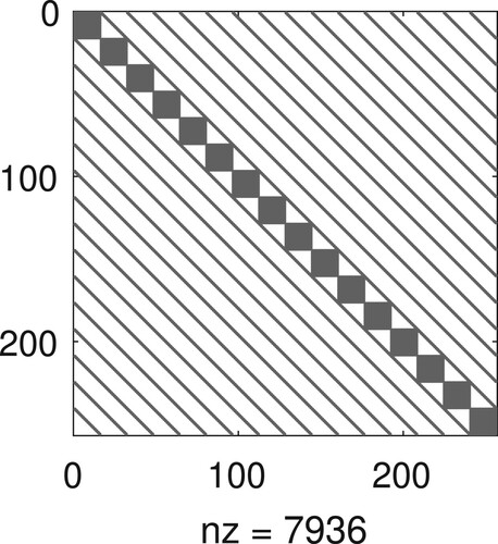The sparse structure of ${\mathbf{M}}_m$ can be seen in Figure 1.

Figure 1. Sparse structure of matrix ${\mathbf{M}}_{\mathbf{m}}$, for n + 1 = 16 grid points on both directions.

As an example to illustrate the effectiveness of the Chebyshev pseudospectral method in conjunction with Crank–Nicolson method, we consider a heat conduction model (1(1) $C(x,y)\frac{\mathrm{\partial }T}{\mathrm{\partial }t}(x,y,t)=\mathrm{\nabla }\cdot [K(x,y)\mathrm{\nabla }T(x,y,t)]+g(x,y,t)\mathrm{in}\mathrm{region}\mathrm{\Gamma }\times (0,\overline{t}],$(1) )–(6(6) $T(x,y,0)=T_0(x,y)\mathrm{in}\mathrm{region}\mathrm{\Gamma }.$(6) ) on $\mathrm{\Gamma }=(0,1)\times (0,1)$, $0\le t\le \overline{t}=1$, extracted from [21], whose solution is given by (40) $T(x,y,t)=(1-e^{-t})(\sin (\pi x)\sin (\pi y)+(\pi +1)(x+y)),$(40) for input data $\begin{array}{rl}{f}_1(y,t)& =\frac{1+y}{12}(1-e^{-t})(\pi \sin (\pi y)+\pi +1),\\ f_2(y,t)& =-\frac{2+y}{12}(1-e^{-t})(-\pi \sin (\pi y)+\pi +1),\\ f_3(x,t)& =\frac{1+x}{12}(1-e^{-t})(\pi \sin (\pi x)+\pi +1),\\ f_4(x,t)& =-\frac{2+x}{12}(1-e^{-t})(-\pi \sin (\pi x)+\pi +1),\\ h_2(y)& =h_4(x)=0,\end{array}$ source term $\begin{array}{rl}g(x,y,t)& =(e^{-t}+\frac{{\pi }^2}{6}(1+x+y)(1-e^{-t}))\sin (\pi x)\sin (\pi y)+\\ & +(\pi +1)e^{-t}(x+y)-\frac{1-e^{-t}}{12}(\pi \sin (\pi (x+y))+2\pi +2),\end{array}$ capacity C = 1, and conductivity given by $k(x,y)=\frac{1+x+y}{12}.$ For this example, we calculate approximate solutions as well as the associated errors with respect to the exact solution of (1(1) $C(x,y)\frac{\mathrm{\partial }T}{\mathrm{\partial }t}(x,y,t)=\mathrm{\nabla }\cdot [K(x,y)\mathrm{\nabla }T(x,y,t)]+g(x,y,t)\mathrm{in}\mathrm{region}\mathrm{\Gamma }\times (0,\overline{t}],$(1) )–(6(6) $T(x,y,0)=T_0(x,y)\mathrm{in}\mathrm{region}\mathrm{\Gamma }.$(6) ). 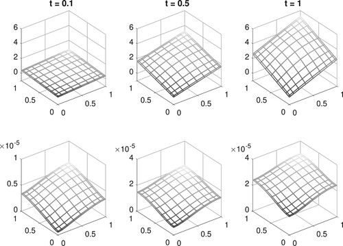CPM is implemented with n + 1 = 11 grid points in both horizontal and vertical directions, $\alpha =0$ and CN runs with time step $\mathrm{\Delta }t=0.01$. Numerical results for three time stages are shown in Figure 2. The accuracy of the approximate solutions is evident when we inspect the pointwise errors at the bottom of the figure.

Figure 2. Numerical solutions for three time stages (top) and associated pointwise absolute error (bottom).

To better evaluate the accuracy of the fully discrete method, we calculate normwise errors in the maximum norm defined by (41) $E_q=||{\mathbf{T}}^{(q)}-\mathbf{T}(t_q){\Vert }_{\mathrm{\infty }}\doteq \underset{k}{max}|[{\mathbf{T}}^{(q)}-\mathbf{T}(t_q){]}_k|,$(41) where $\mathbf{T}(t)$ has entries $T(x_i,y_j,t)$ with gridpoints $(x_i,y_j)$ in lexicographic order. For $q=10,q=50$ and $q=100,$ which correspond to $t=0.1,t=0.5$ and t = 1, respectively, we obtain $E_{10}=5.9071\times {10}^{-6},E_{50}=2.1342\times {10}^{-5}\mathrm{and}{E}_{100}=3.0597\times {10}^{-5}.$ The errors not only verify the theoretical accuracy predicted in theory, but also the potentiality of the proposed method of providing approximate solutions, with relatively high accuracy, using few grid points and therefore at low cost.

3. Numerical method for the inverse problem – isotropic case

Based on the solver for the direct problem described in the previous section, we will now introduce a method for solving the associated inverse problem, namely the conductivity estimation problem from measured transient data. For the numerical treatment of the inverse problem, unknowns values $k(x_i,y_j)$ are arranged in a vector, say $\mathbf{k}$, and function values T (temperature or electrostatic potential) are regarded as functions of $\mathbf{k}$. Assuming that the unknowns are ordered like functions values, let (42) $\ell =i+j(n+1)+1,i=0,1,\dots ,n,j=0,1,\dots ,n.$(42) It is clear that for each unknown $k(x_i,y_j)$ there is a unique entry ${\mathbf{k}}_{\ell }$ of $\mathbf{k}$ so that the lexicographic ordering of the grid $(x_i,y_j)$, as illustrated in Figure 3, is preserved in the entries of $\mathbf{k}$. The ordering in ${\mathbf{k}}_{\ell }$ is taken into account when implementing the inverse problem approach to be described below. The objective of this section is to determine conductivity values $\mathbf{k}$ from measured temperature values $\stackrel{\mathsf{~}}{\mathsf{T}}=\mathsf{\text{T}}+e$, where e denotes an unknown perturbation term and $\mathsf{\text{T}}$ is a vector of exact temperature values on the grid at time steps $t_q,q=1,\dots ,N$, (43) $\mathsf{\text{T}}=\left[\begin{array}{c}\mathbf{T}(t_1)\\ ⋮\\ \mathbf{T}(t_N)\end{array}\right]\in {\mathbb{R}}^{N(n+1{)}^2},$(43) where $\mathbf{T}(t_q)\in {\mathbb{R}}^{(n+1{)}^2}$ has entries $T_{\ell }^{(t_q)}\doteq T(x_i,y_j,t_q)$ with ℓ defined in (42(42) $\ell =i+j(n+1)+1,i=0,1,\dots ,n,j=0,1,\dots ,n.$(42) ) and $(x_i,y_j)$ following the lexicographic ordering. Similar observations apply to $\stackrel{\mathsf{~}}{\mathsf{T}}$. We will assume that an estimate of the error e is available such that (44) $\Vert \stackrel{\mathsf{~}}{\mathsf{T}}-\mathsf{\text{T}}\Vert =\Vert e\Vert \le \delta ,$(44) though, of course, this may not be the case when dealing with reconstruction problems based on experimental measurements. If not, it is essential that the error $\Vert e\Vert$ be estimated either based on prior knowledge or by other means. In addition, observe that, under mild conditions, for each $\mathbf{k}$ we can solve the direct problem (36(36) $\{\begin{array}{l}\mathbf{C}{\displaystyle \frac{\mathrm{d}\mathbf{T}}{\mathrm{d}t}}=\hat{\mathbf{H}}(t,\mathbf{T}),t\in (0,\overline{t}]\\ \mathbf{T}(0)={\mathbf{T}}^0\end{array},$(36) ) to produce a related solution $\mathbf{T}(\mathbf{k},t)$ which contains approximations to $T(x_i,y_j,t)$ on the grid, and hence, a vector $\mathsf{\text{T}}(\mathbf{k})$ with entries $T_{\ell }^{(t_q)}(\mathbf{k})$. With this observation in mind the conductivity estimation problem can be formulated as one of estimating a vector $\mathbf{k}$ such that the difference between computed solutions $\mathsf{\text{T}}(\mathbf{k})$, and measured transient data $\stackrel{\mathsf{~}}{\mathsf{T}}$ is small enough in some sense. More precisely, the estimation problem can be formulated as the non-linear least squares problem of finding ${\mathbf{k}}^{\ast }$ such that (45) ${\mathbf{k}}^{\ast }=\underset{\mathbf{k}\in {\mathbb{R}}^{(n+1{)}^2}}{\mathrm{argmin}}\varphi (\mathbf{k}),\varphi (\mathbf{k})=\frac{1}{2}\Vert \mathsf{\text{T}}(\mathbf{k})-\stackrel{\mathsf{~}}{\mathsf{T}}{\Vert }_2^2=\frac{1}{2}\sum _{j=1}^N\sum _{\ell =1}^{(n+1{)}^2}{(T_{\ell }^{(t_j)}(\mathbf{k})-{\tilde{T}}_{\ell }^{(t_j)})}^2,$(45) where $\mathbf{k}=[{\mathbf{k}}_1,\dots ,{\mathbf{k}}_{(n+1{)}^2}{]}^{\mathrm{T}}$ is the vector of unknowns. The non-linear problem (45(45) ${\mathbf{k}}^{\ast }=\underset{\mathbf{k}\in {\mathbb{R}}^{(n+1{)}^2}}{\mathrm{argmin}}\varphi (\mathbf{k}),\varphi (\mathbf{k})=\frac{1}{2}\Vert \mathsf{\text{T}}(\mathbf{k})-\stackrel{\mathsf{~}}{\mathsf{T}}{\Vert }_2^2=\frac{1}{2}\sum _{j=1}^N\sum _{\ell =1}^{(n+1{)}^2}{(T_{\ell }^{(t_j)}(\mathbf{k})-{\tilde{T}}_{\ell }^{(t_j)})}^2,$(45) ) can be handled in a number of ways, e.g. by using Tikhonov regularization, trust region methods, nonmonotone line search methods, Levenberg–Marquardt method (LMM), or others, see, e.g. [37–40], though clearly the presence of multiple minima cannot be ruled out.

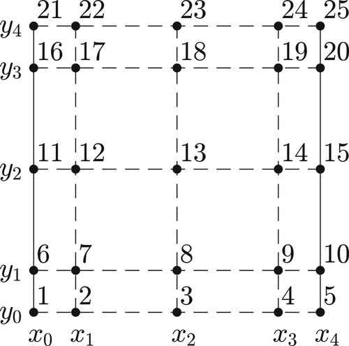
Figure 3. Example of grid, for n = 4, enumerated in accordance with Equation (42(42) $\ell =i+j(n+1)+1,i=0,1,\dots ,n,j=0,1,\dots ,n.$(42) ), i.e, lexicographic order.

In this work, we choose to apply the Levenberg–Marquardt method (LMM), following a version described by Yamashita and Fukushima [32] who consider LMM with line search and Armijo stepsize rule. To simplify the notation, we set $\varphi (\mathbf{k})=\frac{1}{2}\Vert \mathcal{F}(\mathbf{k}){\Vert }_2^2$, and observe that the first-order necessary condition for minimization of φ, $\mathrm{\nabla }\varphi (\mathbf{k})=0,$ reads (46) ${{\mathcal{F}}^{\prime }}^{\mathrm{T}}(\mathbf{k})[\mathsf{\text{T}}(\mathbf{k})-\stackrel{\mathsf{~}}{\mathsf{T}}]=0,$(46) where ${\mathcal{F}}^{\prime }(\mathbf{k})$ denotes derivative of $\mathcal{F}(\mathbf{k})$. LMM minimizes iteratively $\varphi (\mathbf{k})$ (hence solves approximately (46(46) ${{\mathcal{F}}^{\prime }}^{\mathrm{T}}(\mathbf{k})[\mathsf{\text{T}}(\mathbf{k})-\stackrel{\mathsf{~}}{\mathsf{T}}]=0,$(46) )) by determining an estimate, say $\hat{\mathbf{k}}$, such that $\Vert {{\mathcal{F}}^{\prime }}^{\mathrm{T}}(\hat{\mathbf{k}})[\mathsf{\text{T}}(\hat{\mathbf{k}})-\stackrel{\mathsf{~}}{\mathsf{T}}]{\Vert }_2$ is small enough. Roughly speaking, chosen an initial guess ${\mathbf{k}}^0$, the underlying idea of LMM is to determine a minimizer of $\varphi (\mathbf{k})$ iteratively by solving a sequence of linear problems of the form (47) $({\mathcal{F}}^{\prime \mathrm{T}}({\mathbf{k}}^j){\mathcal{F}}^{\prime }({\mathbf{k}}^j)+{\mu }^j{\mathrm{\Omega }}^j)\mathbf{d}=-{\mathcal{F}}^{\prime \mathrm{T}}({\mathbf{k}}^j)\mathcal{F}({\mathbf{k}}^j),j=0,1,\dots ,$(47) where ${\mu }^j$ is the so-called damping parameter and ${\mathrm{\Omega }}^j$ is a diagonal matrix with positive entries. Yamashita and Fukushima choose ${\mathrm{\Omega }}^j$ as the identity matrix and the damping parameter ${\mu }^j$ as the squared residual norm at iteration j. This version can be described as follows.

• LMM with line search

• Step 0: choose parameters $\nu ,\eta ,\gamma \in (0,1)$ and a initial guess ${\mathbf{k}}^0\in {\mathbb{R}}^{(n+1{)}^2}$. Set j = 0 and ${\mu }^0=\Vert \mathcal{F}({\mathbf{k}}^0){\Vert }_2^2$.

• Step 1: If ${\mathbf{k}}^j$ satisfies some termination criterion, stop. Else, go to Step 2.

• Step 2: Find the solution ${\mathbf{d}}^j$ of the system of linear equations (47(47) $({\mathcal{F}}^{\prime \mathrm{T}}({\mathbf{k}}^j){\mathcal{F}}^{\prime }({\mathbf{k}}^j)+{\mu }^j{\mathrm{\Omega }}^j)\mathbf{d}=-{\mathcal{F}}^{\prime \mathrm{T}}({\mathbf{k}}^j)\mathcal{F}({\mathbf{k}}^j),j=0,1,\dots ,$(47) ). If ${\mathbf{d}}^j$ satisfies $\Vert \mathcal{F}({\mathbf{k}}^j+{\mathbf{d}}^j){\Vert }_2\le \gamma \Vert \mathcal{F}({\mathbf{k}}^j){\Vert }_2,$then ${\mathbf{k}}^{j+1}={\mathbf{k}}^j+{\mathbf{d}}^j$ and go to Step 4. Otherwise, go to Step 3.

• Step 3: (Armijo's rule) Take m as the smallest nonnegative integer such that $\varphi ({\mathbf{k}}^j+{\eta }^m{\mathbf{d}}^j)-\varphi ({\mathbf{k}}^j)\le \nu {\eta }^m\mathrm{\nabla }\varphi ({\mathbf{k}}^j{)}^{\mathrm{T}}{\mathbf{d}}^j$and set ${\mathbf{k}}^{j+1}={\mathbf{k}}^j+{\eta }^m{\mathbf{d}}^j$.

• Step 4: Set ${\mu }^{j+1}=\Vert \mathcal{F}({\mathbf{k}}^{j+1}){\Vert }_2^2$ and j = j + 1. Go to Step 1.

As already mentioned, in this work ${\mathrm{\Omega }}^j$ in (47(47) $({\mathcal{F}}^{\prime \mathrm{T}}({\mathbf{k}}^j){\mathcal{F}}^{\prime }({\mathbf{k}}^j)+{\mu }^j{\mathrm{\Omega }}^j)\mathbf{d}=-{\mathcal{F}}^{\prime \mathrm{T}}({\mathbf{k}}^j)\mathcal{F}({\mathbf{k}}^j),j=0,1,\dots ,$(47) ) is replaced by a product of the form ${\mathbf{R}}^{\mathrm{T}}\mathbf{R}$, in a way that ${\mathbf{d}}^j$ is computed by solving the ‘scaled’ system (48) $({\mathcal{F}}^{\prime \mathrm{T}}({\mathbf{k}}^j){\mathcal{F}}^{\prime }({\mathbf{k}}^j)+{\mu }^j{\mathbf{R}}^{\mathrm{T}}\mathbf{R}\mathbf{)}\mathbf{d}\mathbf{=}\mathbf{-}{\mathcal{F}}^{\prime \mathrm{T}}\mathbf{(}{\mathbf{k}}^{\mathbf{j}}\mathbf{)}\mathcal{F}\mathbf{(}{\mathbf{k}}^{\mathbf{j}}\mathbf{)}\mathbf{,}$(48) where $\mathbf{R}$ is a 2D discrete differentiation operator referred to as regularization matrix, $\mathbf{R}\doteq {\mathcal{L}}_i,$ (49) ${\mathcal{L}}_i=\left[\begin{array}{c}{I}_{n+1}\otimes L_i(n+1)\\ L_i(n+1)\otimes I_{n+1}\end{array}\right],i=1,2,$(49) with matrices $L_1(m)\in {\mathbb{R}}^{(m-1)\times m}$ and $L_2(m)\in {\mathbb{R}}^{(m-2)\times m}$ given by $L_1(m)=\left[\begin{array}{cccc}-1& 1& & \\ & \ddots & \ddots & \\ & & -1& 1\end{array}\right]\mathrm{and}{L}_2(m)=\left[\begin{array}{ccccc}1& -2& 1& & \\ & \ddots & \ddots & \ddots & \\ & & 1& -2& 1\end{array}\right].$ Matrices $L_1$ and $L_2$ represent, respectively, the 1D first and second order discrete differentiation operator; they are often employed in image reconstruction problems [41]. Such a modification is introduced to incorporate in the iterative process smoothing properties of conductivity in the horizontal and vertical directions, as well as to provide the reader with further insight into the role that the regularizer matrix plays into the stabilization of the inverse problem. Illustrative numerical examples are postponed to next sections.

3.1. Jacobian matrix

To apply Step 2 above, it is mandatory the calculation of the derivative of $\mathcal{F}$ with respect to $\mathbf{k}$, that depends, implicitly, on the derivative of $\mathbf{T}$ with respect to the same variable. Variation of $\mathbf{T}$ as a function of $\mathbf{k}$ at time step t is determined by the Jacobian of $\mathbf{T}$ denoted here by $\mathbf{J}(t)$, $\mathbf{J}(t)=[\frac{\mathrm{\partial }\mathbf{T}}{\mathrm{\partial }{\mathbf{k}}_1}(\mathbf{k},t),\dots ,\frac{\mathrm{\partial }\mathbf{T}}{\mathrm{\partial }{\mathbf{k}}_{(n+1{)}^2}}(\mathbf{k},t)].$ It can be calculated as follows. Taking derivative with respect to ${\mathbf{k}}_{\ell }$ on both sides of (36(36) $\{\begin{array}{l}\mathbf{C}{\displaystyle \frac{\mathrm{d}\mathbf{T}}{\mathrm{d}t}}=\hat{\mathbf{H}}(t,\mathbf{T}),t\in (0,\overline{t}]\\ \mathbf{T}(0)={\mathbf{T}}^0\end{array},$(36) ) and assuming continuity of $\mathbf{T}$ leads to (50) $\mathbf{C}{\displaystyle \frac{\mathrm{d}}{\mathrm{d}t}}(\frac{\mathrm{\partial }\mathbf{T}}{\mathrm{\partial }{\mathbf{k}}_{\ell }}(\mathbf{k},t))=\frac{\mathrm{\partial }\mathbf{M}}{\mathrm{\partial }{\mathbf{k}}_{\ell }}\mathbf{T}(\mathbf{k},t)+\mathbf{M}\frac{\mathrm{\partial }\mathbf{T}}{\mathrm{\partial }{\mathbf{k}}_{\ell }}(\mathbf{k},t),$(50) where $\mathbf{M}$ denotes the matrix in (38(38) $\mathbf{M}=\left(\begin{array}{cccc}{\hat{\mathbf{F}}}_0& & & \\ & {\hat{\mathbf{F}}}_1& & \\ & & \ddots & \\ & & & {\hat{\mathbf{F}}}_n\end{array}\right)+\mathbf{P}\left(\begin{array}{cccc}{\hat{\mathbf{G}}}_0& & & \\ & {\hat{\mathbf{G}}}_1& & \\ & & \ddots & \\ & & & {\hat{\mathbf{G}}}_n\end{array}\right){\mathbf{P}}^{\mathrm{T}},$(38) ). Now, since initial values of $\mathbf{T}$ do not depend on $\mathbf{k}$, it follows that the ℓ-th column of the Jacobian matrix solves the IVP (51) $\{\begin{array}{l}\mathbf{C}{\displaystyle \frac{\mathrm{d}}{\mathrm{d}t}}({\displaystyle \frac{\mathrm{\partial }\mathbf{T}}{\mathrm{\partial }{\mathbf{k}}_{\ell }}}(\mathbf{k},t))=\mathbf{M}{\displaystyle \frac{\mathrm{\partial }\mathbf{T}}{\mathrm{\partial }{\mathbf{k}}_{\ell }}}(\mathbf{k},t)+{\mathbf{W}}_{\ell }(t)\\ {\displaystyle \frac{\mathrm{\partial }\mathbf{T}}{\mathrm{\partial }{\mathbf{k}}_{\ell }}}(\mathbf{k},0)=0\end{array},$(51) where (52) ${\mathbf{W}}_{\ell }(t)=\frac{\mathrm{\partial }\mathbf{M}}{\mathrm{\partial }{\mathbf{k}}_{\ell }}\mathbf{T}(\mathbf{k},t),\ell =1,2,\dots ,(n+1{)}^2.$(52) Therefore, computing the columns of the Jacobian matrix requires solving a sequence of IVPs with distinct source terms ${\mathbf{W}}_{\ell }(t)$, the computation of which is straightforward. In fact, it is not difficult to see that $\begin{array}{rl}\frac{\mathrm{\partial }\mathbf{M}}{\mathrm{\partial }{\mathbf{k}}_1}& =[\left(\begin{array}{clll}\alpha d_0{r}_0^{\mathrm{T}}& & & \\ & \mathbf{0}& & \\ & & \ddots & \\ & & & \mathbf{0}\end{array}\right)+\mathbf{P}\left(\begin{array}{clll}\alpha d_0{r}_0^{\mathrm{T}}& & & \\ & \mathbf{0}& & \\ & & \ddots & \\ & & & \mathbf{0}\end{array}\right){\mathbf{P}}^{\mathrm{T}}],\\ \frac{\mathrm{\partial }\mathbf{M}}{\mathrm{\partial }{\mathbf{k}}_2}& =[\left(\begin{array}{rlll}{d}_1{r}_1^{\mathrm{T}}& & & \\ & \mathbf{0}& & \\ & & \ddots & \\ & & & \mathbf{0}\end{array}\right)+\mathbf{P}\left(\begin{array}{rlll}\mathbf{0}& & & \\ & \alpha d_0{r}_0^{\mathrm{T}}& & \\ & & \ddots & \\ & & & \mathbf{0}\end{array}\right){\mathbf{P}}^{\mathrm{T}}],\\ & ⋮\\ \frac{\mathrm{\partial }\mathbf{M}}{\mathrm{\partial }{\mathbf{k}}_{n+1}}& =[\left(\begin{array}{rlll}\alpha d_n{r}_n^{\mathrm{T}}& & & \\ & \mathbf{0}& & \\ & & \ddots & \\ & & & \mathbf{0}\end{array}\right)+\mathbf{P}\left(\begin{array}{rlll}\mathbf{0}& & & \\ & \mathbf{0}& & \\ & & \ddots & \\ & & & \alpha d_0{r}_0^{\mathrm{T}}\end{array}\right){\mathbf{P}}^{\mathrm{T}}].\end{array}$ Derivatives with respect to the remaining parameters are calculated similarly. Summarizing, to apply LMM we compute ${\mathcal{F}}^{\prime }(\mathbf{k})$ at every needed time step, which is done by solving IVPs (51(51) $\{\begin{array}{l}\mathbf{C}{\displaystyle \frac{\mathrm{d}}{\mathrm{d}t}}({\displaystyle \frac{\mathrm{\partial }\mathbf{T}}{\mathrm{\partial }{\mathbf{k}}_{\ell }}}(\mathbf{k},t))=\mathbf{M}{\displaystyle \frac{\mathrm{\partial }\mathbf{T}}{\mathrm{\partial }{\mathbf{k}}_{\ell }}}(\mathbf{k},t)+{\mathbf{W}}_{\ell }(t)\\ {\displaystyle \frac{\mathrm{\partial }\mathbf{T}}{\mathrm{\partial }{\mathbf{k}}_{\ell }}}(\mathbf{k},0)=0\end{array},$(51) ) for all source terms. For clarity purposes, observe that, because $\mathsf{\text{T}}$ is vector in ${\mathbb{R}}^{N(n+1{)}^2}$ with block entries $\mathbf{T}(t_i)$, $i=1,\dots ,N$, as described in  (43(43) $\mathsf{\text{T}}=\left[\begin{array}{c}\mathbf{T}(t_1)\\ ⋮\\ \mathbf{T}(t_N)\end{array}\right]\in {\mathbb{R}}^{N(n+1{)}^2},$(43) ), it is easy to see that ${\mathcal{F}}^{\prime }(\mathbf{k})=\left[\begin{array}{c}{\mathbf{J}}_1\\ {\mathbf{J}}_2\\ ⋮\\ {\mathbf{J}}_N\end{array}\right],$ where ${\mathbf{J}}_q=\mathbf{J}(t_q)$ represents the Jacobian of $\mathbf{T}$ with respect to $\mathbf{k}$ at time step $t_q$, for $q=1,2,\dots ,N$. We recall that the computation of ${\mathbf{J}}_q$ demands to solve a sequence of $(n+1{)}^2$ IVPs and, in this sense, for large problems, it may be interesting to use parallel computing, in order to reduce operational time along with memory usage.

3.2. Numerical experiments

We report the outcome of numerical experiments to illustrate the effectiveness of the proposed reconstruction method on some test problems using synthetic data. To this end, noisy measurements are simulated by adding random noise to actual data $T(x_i,y_j,t_q)$ and arranged in a vector data $\stackrel{\mathsf{~}}{\mathsf{T}}=\mathsf{\text{T}}+e$, with $\mathsf{\text{T}}$ defined in (43(43) $\mathsf{\text{T}}=\left[\begin{array}{c}\mathbf{T}(t_1)\\ ⋮\\ \mathbf{T}(t_N)\end{array}\right]\in {\mathbb{R}}^{N(n+1{)}^2},$(43) ), where e is a vector containing zero-mean random numbers scaled in such a way that (53) $\Vert \stackrel{\mathsf{~}}{\mathsf{T}}-\mathsf{\text{T}}\Vert =\mathrm{NL}\Vert \mathsf{\text{T}}\Vert \le \delta ,$(53) where $\mathrm{NL}$ stands for relative noise level in the data and δ is assumed to be available.

As it is often difficult to get exact solutions of problem (1(1) $C(x,y)\frac{\mathrm{\partial }T}{\mathrm{\partial }t}(x,y,t)=\mathrm{\nabla }\cdot [K(x,y)\mathrm{\nabla }T(x,y,t)]+g(x,y,t)\mathrm{in}\mathrm{region}\mathrm{\Gamma }\times (0,\overline{t}],$(1) )–(6(6) $T(x,y,0)=T_0(x,y)\mathrm{in}\mathrm{region}\mathrm{\Gamma }.$(6) ), in our numerical experiments we will use synthetic data generated by solving the transport model by the finite element method (FEM). For this, the input data will be extracted from [20]. Before proceeding, it is instructive to compare the quality of the solutions obtained by CPM and FEM. To do this, we will use the test problem described at the end of Section 2 whose solution is available. Recall that, when using FEM the domain Γ is discretized using a triangular mesh with $\tilde{N}$ nodes and approximate solutions are determined as (54) $T_h(x,y,t)=\sum _{i=1}^{\tilde{N}}{c}_i(t){\phi }_i(x,y),(x,y,t)\in \mathrm{\Gamma }\times (0,\overline{t}],$(54) where $c_i(t)$ are unknowns to be determined and ${\phi }_i$ are frequently called hat functions, every one being continuous, piecewise linear (a plane inside every element/triangle of the mesh), taking a unit value at the ith node and zero elsewhere. Parameter h stands for the global mesh size, defined as the maximum distance between each pair of nodes in the mesh. Considering $C(x,y)=C$ constant in (1(1) $C(x,y)\frac{\mathrm{\partial }T}{\mathrm{\partial }t}(x,y,t)=\mathrm{\nabla }\cdot [K(x,y)\mathrm{\nabla }T(x,y,t)]+g(x,y,t)\mathrm{in}\mathrm{region}\mathrm{\Gamma }\times (0,\overline{t}],$(1) ), FEM turns Equations (1(1) $C(x,y)\frac{\mathrm{\partial }T}{\mathrm{\partial }t}(x,y,t)=\mathrm{\nabla }\cdot [K(x,y)\mathrm{\nabla }T(x,y,t)]+g(x,y,t)\mathrm{in}\mathrm{region}\mathrm{\Gamma }\times (0,\overline{t}],$(1) )–(6(6) $T(x,y,0)=T_0(x,y)\mathrm{in}\mathrm{region}\mathrm{\Gamma }.$(6) ) into the semidiscrete model (55) $\{\begin{array}{l}C\stackrel{\mathbf{~}}{\mathbf{M}}{\displaystyle \frac{\mathrm{d}\mathbf{c}}{\mathrm{d}t}}+\stackrel{\mathbf{~}}{\mathbf{A}}\mathbf{c}=\tilde{\mathbf{f}}(t),t\in (0,\overline{t}]\\ \mathbf{c}(0)=0\end{array},$(55) where $\mathbf{c}(t)=(c_1(t),\dots ,c_{\tilde{N}}(t){)}^{\mathrm{T}}$, $\stackrel{\mathbf{~}}{\mathbf{M}}$ and $\stackrel{\mathbf{~}}{\mathbf{A}}$ are $\tilde{N}\times \tilde{N}$ known as mass and stiffness matrices, resp., and $\tilde{\mathbf{f}}(t)$ contains other independent terms. For more information on FEM discretization, see, for example, Johnson [42] and Larson and Bengzon [43].

To proceed, in a similar way as the semi-discrete problem associated with CPM was solved in Section 2, here the IVP (55(55) $\{\begin{array}{l}C\stackrel{\mathbf{~}}{\mathbf{M}}{\displaystyle \frac{\mathrm{d}\mathbf{c}}{\mathrm{d}t}}+\stackrel{\mathbf{~}}{\mathbf{A}}\mathbf{c}=\tilde{\mathbf{f}}(t),t\in (0,\overline{t}]\\ \mathbf{c}(0)=0\end{array},$(55) ) is also solved by the CN method. This guarantees second-order approximations in space and time, the order in space being in relation to the global mesh size h [42]. We calculate approximate solutions $T_h$ for $h=0.1$ and $h=0.01$ with $\mathrm{\Delta }t=0.01$ for both cases. In practice, for chosen h, a structured mesh with $\tilde{N}$ nodes is generated using MATLAB's PDE toolbox via function initmesh. It is noteworthy mentioning that for the above values of h correspond meshes consisting of $\tilde{N}=185$ and $\tilde{N}=17361$ nodes, respectively. Note that the refinement made on the mesh results in a significant increase in computational cost, since the unknowns of the linear system grow from $\tilde{N}=183$ to $\tilde{N}=17361$, which in addition to making the application of the CN method more expensive, allows for the potential growth of rounding errors. Figure 4 shows a simple mesh, the respective approximate solution $T_h$ at time t = 1 and also the structure of mass matrix, which is repeated in the stiffness matrix, both with density around $3.53\mathrm{\%}$.

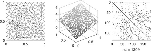
Figure 4. Example of FEM mesh's structure with 185 nodes, 328 triangles and global mesh size h = 0.1 (left), respective solution with CN ($\mathrm{\Delta }t=0.01$) at time t = 1 (middle) and sparse structure of mass matrix $\stackrel{\mathbf{~}}{\mathbf{M}}$ (right), for data used in Figure 2.

Normwise errors in the maximum norm are also calculated and defined by ${\hat{E}}_h(t)=\underset{(x_i,y_j)}{max}|T_h(x_i,y_j,t)-T(x_i,y_j,t)|,$ with $(x_i,y_j)$ varying along the nodes. The errors associated with the approximate solutions $T_h$ for three time stages are shown in Table 1, in which, for comparison purposes, the errors of CPM-based solutions reported in the previous section are also included. The superior performance of CPM is clearly seen in this table, even in the case h = 0.01, which involves working with linear systems of size $17361\times 17361$, as opposed to CPM that deals with systems $121\times 121$. This ends the desired comparison.

Table 1. Errors associated with FEM-based solutions for two global mesh sizes and errors associated with CPM.

t	${\hat{E}}_h(t)$ $(h=0.1)$	${\hat{E}}_h(t)$ $(h=0.01)$	$E_q$ $(n=10)$
0.1	$9.3656\times {10}^{-3}$	$1.2089\times {10}^{-4}$	$5.9071\times {10}^{-6}$
0.5	$2.5849\times {10}^{-2}$	$4.2066\times {10}^{-4}$	$2.1342\times {10}^{-5}$
1.0	$3.6829\times {10}^{-2}$	$6.3101\times {10}^{-4}$	$3.0597\times {10}^{-5}$

We are now in a position to describe some examples of conductivity reconstruction. As already mentioned, in practice, it is difficult to get exact temperature data $T(x,y,t)$ satisfying the conduction model. So, to challenge the reconstruction method, we shall use synthetic data generated by solving the direct problem through the combination of FEM and CN method. All our numerical experiments are conducted using the following input data: (56) $\begin{array}{rl}g(x,y,t)& =0,f_1(y,t)=-1,f_2(y,t)=1,\end{array}$(56) (57) $\begin{array}{rl}{f}_3(x,t)& =-1,f_4(x,t)=1,\mathrm{and}{h}_2(y)=h_4(x)=0,\end{array}$(57) with $\mathrm{\Gamma }=(0,1)\times (0,1)$, $\overline{t}=1$, capacity $C(x,y)=1$, initial condition $T_0(x,y)=0$, with conductivity $k(x,y)$ to be described in consonance with the case/example under consideration. For all examples, we choose $h=0.01=\mathrm{\Delta }t$; Thus, $T_h$ is $\mathcal{O}(h^2)=\mathcal{O}({10}^{-4})$ at each time step and we accept it as a reliable alternative to the lack of exact T. We emphasize that our decision of using FEM instead of CPM to generate data obeys the need to prevent the inverse crime [44,45]: the inverse crime occurs when the same numerical model is used to synthesize as well as to invert data in an inverse problem. For this, in our numerical examples, what we call ‘exact’ data, supposed to satisfy (43(43) $\mathsf{\text{T}}=\left[\begin{array}{c}\mathbf{T}(t_1)\\ ⋮\\ \mathbf{T}(t_N)\end{array}\right]\in {\mathbb{R}}^{N(n+1{)}^2},$(43) ), are values obtained by interpolating $T_h$ in the grid generated by Chebyshev points.

All the reconstruction examples in this section are performed using noisy data $\stackrel{\mathsf{~}}{\mathsf{T}}$ consisting of temperature values on a grid of n + 1 = 16 Chebyshev points associated with N = 5 time steps equally distributed from $0.1$ to $0.5$. We emphasize that, since the number of unknowns is $(n+1{)}^2$ and as the temperature in the entire mesh generates $(n+1{)}^2$ non-linear relations at each stage of time, temperature values of only N = 2 stages are sufficient to make the minimization problem overdetermined. In this case, $N=2$ would be sufficient to determine conductivity estimates. Our choice N = 5 aims to make the minimization problem highly overdetermined to, on the one hand, allow better noise filtering and, on the other hand, expect that the minimization process results in a unique solution. As for LMM, it starts with ${\mathbf{k}}^0$ constant equals to 1/12 along the grid. Other parameters, necessary to LMM, are taken as $\eta =\gamma =0.7$ and $\nu ={10}^{-2}$. For more information about LMM parameters the reader is referred to [46, Section ].

To terminate the estimation process, LMM is stopped by means of the discrepancy principle (DP) [33], i.e. the iterates stop at the first j such that (58) $\Vert \mathsf{\text{T}}({\mathbf{k}}^j)-\stackrel{\mathsf{~}}{\mathsf{T}}{\Vert }_2\le \tau \delta ,\tau >1,$(58) where τ is a safeward parameter intended to prevent underestimation of the data error $\Vert \stackrel{\mathsf{~}}{\mathsf{T}}-\mathsf{\text{T}}\Vert$, see (44(44) $\Vert \stackrel{\mathsf{~}}{\mathsf{T}}-\mathsf{\text{T}}\Vert =\Vert e\Vert \le \delta ,$(44) ). In agreement with this, τ is often chosen close to 1, though the option τ close to 2 be also found in literature, see e.g. [47, Section ]. In this paper, all implementations consider $\tau =1.1$. 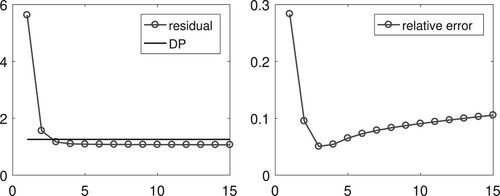DP is commonly used in solving ill-posed problems because the presence of noise in the data generates during the iterations the so-called semi-convergence behaviour [48]. Roughly speaking, while early iterations capture relevant information about the sought solution, as j grows the iterations capture information about the noise, corrupting gradually the iterative process, see Figure 5. Thus, DP is used to select an iterate capable of balancing accuracy and stability on the approximate solution.

Figure 5. Residual $\Vert \mathsf{\text{T}}({\mathbf{k}}^j)-\stackrel{\mathsf{~}}{\mathsf{T}}{\Vert }_2$ (left) and relative error between ${\mathbf{k}}^j$ and the exact conductivity $k(x,y)=(1+x+y)/12$ (right), $\mathrm{NL}=1\mathrm{\%}$.

As for notation on tables and figures, RE denotes the relative error between exact k and the approximation and IE represents the relative error considering just grid points inside the grid, i.e. without nodes on the boundary. The error IE is calculated to evaluate the behaviour of the solutions close to the boundary.

Example 1

Consider conductivity $k(x,y)=(1+x+y)/12$ and noise level $\mathrm{NL}=0.1\mathrm{\%}$. This first example aims to show the influence of different scaling matrices ${\mathbf{R}}^{\mathrm{T}}\mathbf{R}$ introduced in (48(48) $({\mathcal{F}}^{\prime \mathrm{T}}({\mathbf{k}}^j){\mathcal{F}}^{\prime }({\mathbf{k}}^j)+{\mu }^j{\mathbf{R}}^{\mathrm{T}}\mathbf{R}\mathbf{)}\mathbf{d}\mathbf{=}\mathbf{-}{\mathcal{F}}^{\prime \mathrm{T}}\mathbf{(}{\mathbf{k}}^{\mathbf{j}}\mathbf{)}\mathcal{F}\mathbf{(}{\mathbf{k}}^{\mathbf{j}}\mathbf{)}\mathbf{,}$(48) ) on the LMM performance in solving the inverse problem, for different values of α in the modified model (36(36) $\{\begin{array}{l}\mathbf{C}{\displaystyle \frac{\mathrm{d}\mathbf{T}}{\mathrm{d}t}}=\hat{\mathbf{H}}(t,\mathbf{T}),t\in (0,\overline{t}]\\ \mathbf{T}(0)={\mathbf{T}}^0\end{array},$(36) ). Figure 6 compares generated solutions. Note that the effect of increasing α, Figure 6(b, c), is seen as a correction of discontinuities at the edge of the reconstructions. This can be explained as follows. As $\alpha +\beta =1$ with $\alpha ,\beta \ge 0$, a consequence of (33(33) $\begin{array}{rl}{d}_{0}k(x_0,y_j){\displaystyle \frac{\mathrm{\partial }T}{\mathrm{\partial }x}}(x_0,y_j,t)& =\alpha d_{0}k(x_0,y_j){\displaystyle \frac{\mathrm{\partial }T}{\mathrm{\partial }x}}(x_0,y_j,t)+\beta d_{0}k(x_0,y_j){\displaystyle \frac{\mathrm{\partial }T}{\mathrm{\partial }x}}(x_0,y_j,t)\\ & =\alpha d_{0}k(x_0,y_j){\displaystyle \frac{\mathrm{\partial }T}{\mathrm{\partial }x}}(x_0,y_j,t)+\beta d_0{f}_1(y_j,t),\end{array}$(33) )–(34(34) $\begin{array}{rl}{d}_{n}k(x_n,y_j){\displaystyle \frac{\mathrm{\partial }T}{\mathrm{\partial }x}}(x_n,y_j,t)& =\alpha d_{n}k(x_n,y_j){\displaystyle \frac{\mathrm{\partial }T}{\mathrm{\partial }x}}(x_n,y_j,t)+\beta d_{n}k(x_n,y_j){\displaystyle \frac{\mathrm{\partial }T}{\mathrm{\partial }x}}(x_n,y_j,t)\\ & =\alpha d_{0}k(x_0,y_j){\displaystyle \frac{\mathrm{\partial }T}{\mathrm{\partial }x}}(x_0,y_j,t)\\ & +\beta [h_2(y_j)T(x_n,y_j,t)d_n-f_2(y_j,t)d_n].\end{array}$(34) ) is that, if on the one hand $\alpha \approx 1$ strengthens the conductivity values $k(x,y)$ on the boundaries, on the other hand, $\beta =1-\alpha \approx 0$ weakens the influence of both the source term and boundary conditions in the model, see again (33(33) $\begin{array}{rl}{d}_{0}k(x_0,y_j){\displaystyle \frac{\mathrm{\partial }T}{\mathrm{\partial }x}}(x_0,y_j,t)& =\alpha d_{0}k(x_0,y_j){\displaystyle \frac{\mathrm{\partial }T}{\mathrm{\partial }x}}(x_0,y_j,t)+\beta d_{0}k(x_0,y_j){\displaystyle \frac{\mathrm{\partial }T}{\mathrm{\partial }x}}(x_0,y_j,t)\\ & =\alpha d_{0}k(x_0,y_j){\displaystyle \frac{\mathrm{\partial }T}{\mathrm{\partial }x}}(x_0,y_j,t)+\beta d_0{f}_1(y_j,t),\end{array}$(33) )–(34(34) $\begin{array}{rl}{d}_{n}k(x_n,y_j){\displaystyle \frac{\mathrm{\partial }T}{\mathrm{\partial }x}}(x_n,y_j,t)& =\alpha d_{n}k(x_n,y_j){\displaystyle \frac{\mathrm{\partial }T}{\mathrm{\partial }x}}(x_n,y_j,t)+\beta d_{n}k(x_n,y_j){\displaystyle \frac{\mathrm{\partial }T}{\mathrm{\partial }x}}(x_n,y_j,t)\\ & =\alpha d_{0}k(x_0,y_j){\displaystyle \frac{\mathrm{\partial }T}{\mathrm{\partial }x}}(x_0,y_j,t)\\ & +\beta [h_2(y_j)T(x_n,y_j,t)d_n-f_2(y_j,t)d_n].\end{array}$(34) ). Clearly, a reverse effect should occur when $\alpha \approx 0$. This suggests that an appropriate balance between α and β is needed, and this is what the numerical results seem to show as α increases starting from values close to zero. However, finding such a balance is difficult since, as it can be seen in Table 2, as α increases, the number of iterations increases as well, bringing instability to the iterates and not significantly reducing the relative error. On the other hand, Figure 6(d,e) presents the regularizing effect of ${\mathcal{L}}_1$ and ${\mathcal{L}}_2$ from (49(49) ${\mathcal{L}}_i=\left[\begin{array}{c}{I}_{n+1}\otimes L_i(n+1)\\ L_i(n+1)\otimes I_{n+1}\end{array}\right],i=1,2,$(49) ), smoothing up the solutions, both in interior and boundary, even with $\alpha =0.1$, at a fairly small number of iterations. Tests for bigger/smaller α brought small changes and were omitted. Table 2 summarizes the results. In resume, the information we emphasize is that a good choice of the regularizer $\mathbf{R}$ can lead to good results, while reducing computational effort.

Figure 6. Comparison between solutions for $k(x,y)=(1+x+y)/12$ calculated with different choices of $\mathbf{R}$ and α. For (d) and (e), $\alpha =0.1$.

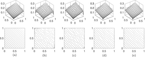
Table 2. Errors and number of iterations until DP is satisfied, for different choices of $\mathbf{R}$ and α, considering as exact $k(x,y)=(1+x+y)/12$.

$\mathbf{R}$	I	I	${\mathcal{L}}_1$	${\mathcal{L}}_2$
α	0.1	0.35	0.1	0.1
RE	0.0946	0.0717	0.0128	0.0134
IE	0.0236	0.0250	0.0096	0.0084
Iterations	7	29	4	4

Example 2

Consider again noise level $\mathrm{NL}=0.1\mathrm{\%}$ and take $\alpha =0.1$ fixed. To assess the effectiveness of the proposed method we choose four different conductivities, namely: $\begin{array}{rl}{k}_1(x,y)& =(1+x^2+y^2)/12,\\ k_2(x,y)& =(1+y^3)/12,\\ k_3(x,y)& =(1+\sin (x)\sin (y))/12\mathrm{and}\\ k_4(x,y)& =(1+\sin (2\pi x{)}^2\sin (2\pi y{)}^2)/12,\end{array}$ where the regularizer is taken as $\mathbf{R}={\mathcal{L}}_2$. Considering the results in Figure 4, it is observed that the use of $\mathbf{R}$ produces smoothing effect on the calculated solutions $\mathbf{k}$, while reducing unwanted artefacts both at the boundary and inside Γ. Results are summarized in Figure 7 and Table 3. Observe the good fitting between the sought solution and the reconstruction, with small number of iterations, contributing on the numerical applications, especially bearing in mind that calculating the Jacobian may become expensive.

Figure 7. Contour plots for every exact $k_i(x,y)$ (top) and the respective approximation (bottom), $i=1,\dots ,4$.

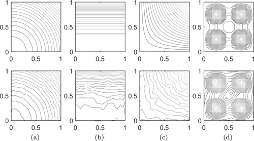
Table 3. Relative errors RE, interior error IE and number of LMM iterations until DP is satisfied.

Function	$k_1(x,y)$	$k_2(x,y)$	$k_3(x,y)$	$k_4(x,y)$
RE	0.0151	0.0196	0.0300	0.0320
IE	0.0093	0.0117	0.0130	0.0310
Iterations	4	3	3	2

Example 3

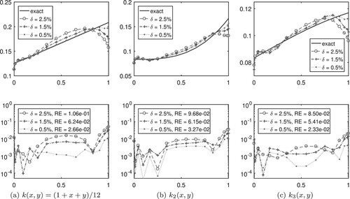
This last example refers to the reconstruction of three conductivities namely, k used in Example 1 and $k_2$, $k_3$ of the previous example, for different noise levels in the data. To this end we set $\mathbf{R}={\mathcal{L}}_2$, $\alpha =0.1$ and choose three values for NL: 2.5%, 1.5% and 0.5%. In Figure 8, top, we show reconstructions of the lines $k(0.5,y)$, $k_2(0.5,y)$ and $k_3(0.5,y),$ while at the bottom, we show relative reconstruction errors on the whole mesh. The numerical results confirm what is often seen in solving inverse problems: as NL gets smaller, so does the reconstruction error.

Figure 8. Behavior of reconstruction results solution for different noise levels. Top: exact conductivities and respective approximations along the line x = 0.5. Bottom: absolute value of reconstruction errors along the line x = 0.5 and relative error RE.

4. Numerical method for the inverse problem – orthotropic case

We now consider the conduction problem (1(1) $C(x,y)\frac{\mathrm{\partial }T}{\mathrm{\partial }t}(x,y,t)=\mathrm{\nabla }\cdot [K(x,y)\mathrm{\nabla }T(x,y,t)]+g(x,y,t)\mathrm{in}\mathrm{region}\mathrm{\Gamma }\times (0,\overline{t}],$(1) )–(6(6) $T(x,y,0)=T_0(x,y)\mathrm{in}\mathrm{region}\mathrm{\Gamma }.$(6) ) focusing on the orthotropic case, i.e.with conductivity tensor $K(x,y)=\left[\begin{array}{cc}{k}_{11}(x,y)& 0\\ 0& k_{22}(x,y)\end{array}\right],$ and we first describe the Chebyshev pseudospectral method used to solve the direct problem. To this end rewrite (1(1) $C(x,y)\frac{\mathrm{\partial }T}{\mathrm{\partial }t}(x,y,t)=\mathrm{\nabla }\cdot [K(x,y)\mathrm{\nabla }T(x,y,t)]+g(x,y,t)\mathrm{in}\mathrm{region}\mathrm{\Gamma }\times (0,\overline{t}],$(1) ) as (59) $C(x,y)\frac{\mathrm{\partial }T}{\mathrm{\partial }t}(x,y,t)={\displaystyle \frac{\mathrm{\partial }}{\mathrm{\partial }x}}(k_{11}(x,y){\displaystyle \frac{\mathrm{\partial }T}{\mathrm{\partial }x}}(x,y,t))+{\displaystyle \frac{\mathrm{\partial }}{\mathrm{\partial }y}}(k_{22}(x,y){\displaystyle \frac{\mathrm{\partial }T}{\mathrm{\partial }y}}(x,y,t))+g(x,y,t)$(59) and then note that along the horizontal direction we have a process identical to (17(17) ${\displaystyle \frac{\mathrm{\partial }}{\mathrm{\partial }x}}(k(x_i,y_j){\displaystyle \frac{\mathrm{\partial }T}{\mathrm{\partial }x}}(x_i,y_j,t))\approx e_{i+1}^{\mathrm{T}}D{\mathbf{K}}_j^x{\dot{\mathbf{T}}}_j,i=0,\dots ,n,j=0,1,\dots ,n,$(17) ), changing k by $k_{11}$ in (20(20) ${\mathbf{T}}_j^x=\left[\begin{array}{c}{\displaystyle \frac{\mathrm{\partial }}{\mathrm{\partial }x}}(k(x_0,y_j){\displaystyle \frac{\mathrm{\partial }T}{\mathrm{\partial }x}}(x_0,y_j,t))\\ ⋮\\ {\displaystyle \frac{\mathrm{\partial }}{\mathrm{\partial }x}}(k(x_n,y_j){\displaystyle \frac{\mathrm{\partial }T}{\mathrm{\partial }x}}(x_n,y_j,t))\end{array}\right],j=0,1,\dots ,n.$(20) ), which leads to (60) $\left[\begin{array}{c}{\mathbf{T}}_0^x\\ {\mathbf{T}}_1^x\\ ⋮\\ {\mathbf{T}}_n^x\end{array}\right]\approx \left(\begin{array}{cccc}{\mathbf{F}}_0& & & \\ & {\mathbf{F}}_1& & \\ & & \ddots & \\ & & & {\mathbf{F}}_n\end{array}\right)\left[\begin{array}{c}{\mathbf{T}}_0\\ {\mathbf{T}}_1\\ ⋮\\ {\mathbf{T}}_n\end{array}\right]+\left[\begin{array}{c}{d}_0{f}_1(y_0,t)-d_n{f}_2(y_0,t)\\ d_0{f}_1(y_1,t)-d_n{f}_2(y_1,t)\\ ⋮\\ d_0{f}_1(y_n,t)-d_n{f}_2(y_n,t)\end{array}\right]$(60) where we set ${\mathbf{F}}_j=D_1{\check{\mathbf{K}}}_j{D}_2+h_2(y_j)d_n{e}_{n+1}^{\mathrm{T}}$ with ${\check{\mathbf{K}}}_j=\mathrm{diag}(k_{11}(x_1,y_j),\dots ,k_{11}(x_{n-1},y_j)),j=0,1,\dots ,n,$ and $T(x_i,y_j)$ enumerated in lexicographic order. For approximations in the vertical direction we change k by $k_{22}$ and proceed as before, leading to the initial value problem (61) $\{\begin{array}{l}\mathbf{C}\frac{\mathrm{d}\mathbf{T}}{\mathrm{d}t}=\mathbf{H}(t,\mathbf{T}),t\in (0,\overline{t}]\\ \mathbf{T}(0)={\mathbf{T}}^0\end{array},$(61) where (62) $\mathbf{H}(t,\mathbf{T})=[\left(\begin{array}{cccc}{\mathbf{F}}_0& & & \\ & {\mathbf{F}}_1& & \\ & & \ddots & \\ & & & {\mathbf{F}}_n\end{array}\right)+\mathbf{P}\left(\begin{array}{cccc}{\mathbf{G}}_0& & & \\ & {\mathbf{G}}_1& & \\ & & \ddots & \\ & & & {\mathbf{G}}_n\end{array}\right){\mathbf{P}}^{\mathrm{T}}]\left[\begin{array}{c}{\mathbf{T}}_0\\ {\mathbf{T}}_1\\ ⋮\\ {\mathbf{T}}_n\end{array}\right]+\mathbf{S}(t),$(62) for ${\mathbf{G}}_i=D_1{\hat{\mathbf{K}}}_i{D}_2+h_4(x_i)d_n{e}_{n+1}^{\mathrm{T}},$ with ${\hat{\mathbf{K}}}_i=\mathrm{diag}(k_{22}(x_i,y_1),k_{22}(x_i,y_2),\dots ,k_{22}(x_i,y_{n-1})),i=0,1,\dots ,n,$ and $\mathbf{S}(t)$ being used to accommodate terms which do not involve unknowns. Essentially, blocks of $\mathbf{F}$ and $\mathbf{G}$ contain information related to $k_{11}$ and $k_{22}$, respectively, and the rest is kept unchanged, exactly as in the isotropic case.

It is easy to see that function T does not depend on the values of $k_{11}(x,y)$ when $x=x_0$ and $x=x_n$, due to the incorporation of boundary conditions. The same happens for $k_{22}(x,y)$ at $y=y_0$ and $y=y_n$, and again, an alternative discretization can be applied, for example, by considering a strategy such as in (33(33) $\begin{array}{rl}{d}_{0}k(x_0,y_j){\displaystyle \frac{\mathrm{\partial }T}{\mathrm{\partial }x}}(x_0,y_j,t)& =\alpha d_{0}k(x_0,y_j){\displaystyle \frac{\mathrm{\partial }T}{\mathrm{\partial }x}}(x_0,y_j,t)+\beta d_{0}k(x_0,y_j){\displaystyle \frac{\mathrm{\partial }T}{\mathrm{\partial }x}}(x_0,y_j,t)\\ & =\alpha d_{0}k(x_0,y_j){\displaystyle \frac{\mathrm{\partial }T}{\mathrm{\partial }x}}(x_0,y_j,t)+\beta d_0{f}_1(y_j,t),\end{array}$(33) ) and (34(34) $\begin{array}{rl}{d}_{n}k(x_n,y_j){\displaystyle \frac{\mathrm{\partial }T}{\mathrm{\partial }x}}(x_n,y_j,t)& =\alpha d_{n}k(x_n,y_j){\displaystyle \frac{\mathrm{\partial }T}{\mathrm{\partial }x}}(x_n,y_j,t)+\beta d_{n}k(x_n,y_j){\displaystyle \frac{\mathrm{\partial }T}{\mathrm{\partial }x}}(x_n,y_j,t)\\ & =\alpha d_{0}k(x_0,y_j){\displaystyle \frac{\mathrm{\partial }T}{\mathrm{\partial }x}}(x_0,y_j,t)\\ & +\beta [h_2(y_j)T(x_n,y_j,t)d_n-f_2(y_j,t)d_n].\end{array}$(34) ). Therefore, the semidiscrete model takes the form (63) $\{\begin{array}{l}\mathbf{C}{\displaystyle \frac{d\mathbf{T}}{dt}}=\hat{\mathbf{H}}(t,\mathbf{T}),t\in (0,\overline{t}]\\ \mathbf{T}(0)={\mathbf{T}}^0\end{array},$(63) where (64) $\hat{\mathbf{H}}(t,\mathbf{T})=\mathbf{M}\mathbf{T}+\hat{\mathbf{S}}(t),$(64) and, again following previous notation, (65) $\mathbf{M}=\left(\begin{array}{cccc}{\hat{\mathbf{F}}}_0& & & \\ & {\hat{\mathbf{F}}}_1& & \\ & & \ddots & \\ & & & {\hat{\mathbf{F}}}_n\end{array}\right)+\mathbf{P}\left(\begin{array}{cccc}{\hat{\mathbf{G}}}_0& & & \\ & {\hat{\mathbf{G}}}_1& & \\ & & \ddots & \\ & & & {\hat{\mathbf{G}}}_n\end{array}\right){\mathbf{P}}^{\mathrm{T}},$(65) for $\begin{array}{l}{\hat{\mathbf{F}}}_j=[\hat{D}{\mathbf{K}}_j^{x}D+\beta h_2(y_j)d_n{e}_{n+1}^{\mathrm{T}}],{\mathbf{K}}_j^x=\mathrm{diag}(k_{11}(x_0,y_j),\dots ,k_{11}(x_n,y_j)),j=0,1,\dots n,\\ \\ {\hat{\mathbf{G}}}_i=[\hat{D}{\mathbf{K}}_i^{y}D+\beta h_4(x_i)d_n{e}_{n+1}^{\mathrm{T}}],{\mathbf{K}}_i^y=\mathrm{diag}(k_{22}(x_i,y_0),\dots ,k_{22}(x_i,y_n)),i=0,1,\dots n,\end{array}$ and $\hat{\mathbf{S}}\mathbf{(}\mathbf{t}\mathbf{)}$ accommodating independent terms. Although the notation here is the same as for the isotropic case, the reader should be aware that the variables involved are different. In fact, in the previous sections, ${\mathbf{K}}_j^x$ and ${\mathbf{K}}_i^y$ were related exclusively to k, while in the orthotropic case they involve $k_{11}$ and $k_{22}$. Ultimately, above relations recover the isotropic case by taking $k_{11}=k_{22}=k$.

Remark 1

Although beyond the scope of this paper, we note that a semi-discrete model similar to (63(63) $\{\begin{array}{l}\mathbf{C}{\displaystyle \frac{d\mathbf{T}}{dt}}=\hat{\mathbf{H}}(t,\mathbf{T}),t\in (0,\overline{t}]\\ \mathbf{T}(0)={\mathbf{T}}^0\end{array},$(63) ) for the anisotropic case can be developed analogously. In fact, in this case, Equation (1(1) $C(x,y)\frac{\mathrm{\partial }T}{\mathrm{\partial }t}(x,y,t)=\mathrm{\nabla }\cdot [K(x,y)\mathrm{\nabla }T(x,y,t)]+g(x,y,t)\mathrm{in}\mathrm{region}\mathrm{\Gamma }\times (0,\overline{t}],$(1) ) takes the form $C\frac{\mathrm{\partial }T}{\mathrm{\partial }t}={\displaystyle \frac{\mathrm{\partial }}{\mathrm{\partial }x}}(k_{11}{\displaystyle \frac{\mathrm{\partial }T}{\mathrm{\partial }x}}+k_{12}{\displaystyle \frac{\mathrm{\partial }T}{\mathrm{\partial }y}})+{\displaystyle \frac{\mathrm{\partial }}{\mathrm{\partial }y}}(k_{21}{\displaystyle \frac{\mathrm{\partial }T}{\mathrm{\partial }x}}+k_{22}{\displaystyle \frac{\mathrm{\partial }T}{\mathrm{\partial }y}})+g$ and every derivative can be approximated using CPM as in (25(25) $\left[\begin{array}{c}{\mathbf{T}}_0^x\\ {\mathbf{T}}_1^x\\ ⋮\\ {\mathbf{T}}_n^x\end{array}\right]\approx \left(\begin{array}{cccc}{\mathbf{F}}_0& & & \\ & {\mathbf{F}}_1& & \\ & & \ddots & \\ & & & {\mathbf{F}}_n\end{array}\right)\left[\begin{array}{c}{\mathbf{T}}_0\\ {\mathbf{T}}_1\\ ⋮\\ {\mathbf{T}}_n\end{array}\right]+\left[\begin{array}{c}{d}_0{f}_1(y_0,t)-d_n{f}_2(y_0,t)\\ d_0{f}_1(y_1,t)-d_n{f}_2(y_1,t)\\ ⋮\\ d_0{f}_1(y_n,t)-d_n{f}_2(y_n,t)\end{array}\right],$(25) ) and (29(29) $\left[\begin{array}{c}{\mathbf{T}}_0^y\\ {\mathbf{T}}_1^y\\ ⋮\\ {\mathbf{T}}_n^y\end{array}\right]\approx \mathbf{P}\left(\begin{array}{cccc}{\mathbf{G}}_0& & & \\ & {\mathbf{G}}_1& & \\ & & \ddots & \\ & & & {\mathbf{G}}_n\end{array}\right){\mathbf{P}}^{\mathrm{T}}\left[\begin{array}{c}{\mathbf{T}}_0\\ {\mathbf{T}}_1\\ ⋮\\ {\mathbf{T}}_n\end{array}\right]+\mathbf{P}\left[\begin{array}{c}{d}_0{f}_3(x_0,t)-d_n{f}_4(x_0,t)\\ d_0{f}_3(x_1,t)-d_n{f}_4(x_1,t)\\ ⋮\\ d_0{f}_3(x_n,t)-d_n{f}_4(x_n,t)\end{array}\right].$(29) ).

As for the inverse problem for the orthotropic case, the goal now is to recover conductivities $k_{11}$ and $k_{22}$ based on data values of T contaminated by noise. We start by enumerating variables $k_{11}(x_i,y_j)$ and $k_{22}(x_i,y_j)$ as done before (see Section 3) and arranging them in a vector (66) $\mathbf{k}=\left[\begin{array}{c}{\mathbf{k}}^{11}\\ {\mathbf{k}}^{22}\end{array}\right],{\mathbf{k}}^{11},{\mathbf{k}}^{22}\in {\mathbb{R}}^{(n+1{)}^2},$(66) such that function values $\mathbf{T}$ depend on $\mathbf{k}$. The computation of the Jacobian matrix $\begin{array}{rl}\mathbf{J}(t)& =[\frac{\mathrm{\partial }\mathbf{T}}{\mathrm{\partial }{\mathbf{k}}_1}(\mathbf{k},t),\dots ,\frac{\mathrm{\partial }\mathbf{T}}{\mathrm{\partial }{\mathbf{k}}_{2(n+1{)}^2}}(\mathbf{k},t)]\\ & =[\frac{\mathrm{\partial }\mathbf{T}}{\mathrm{\partial }{\mathbf{k}}_1^{11}}(\mathbf{k},t),\dots ,\frac{\mathrm{\partial }\mathbf{T}}{\mathrm{\partial }{\mathbf{k}}_{(n+1{)}^2}^{11}}(\mathbf{k},t),\frac{\mathrm{\partial }\mathbf{T}}{\mathrm{\partial }{\mathbf{k}}_1^{22}}(\mathbf{k},t),\dots ,\frac{\mathrm{\partial }\mathbf{T}}{\mathrm{\partial }{\mathbf{k}}_{(n+1{)}^2}^{22}}(\mathbf{k},t)]\end{array}$ remains essentially the same, but noting that the problem now has $2(n+1{)}^2$ unknown parameters and that the source terms in (52(52) ${\mathbf{W}}_{\ell }(t)=\frac{\mathrm{\partial }\mathbf{M}}{\mathrm{\partial }{\mathbf{k}}_{\ell }}\mathbf{T}(\mathbf{k},t),\ell =1,2,\dots ,(n+1{)}^2.$(52) ) change accordingly. Of course, if $\mathbf{M}$ is the matrix in (65(65) $\mathbf{M}=\left(\begin{array}{cccc}{\hat{\mathbf{F}}}_0& & & \\ & {\hat{\mathbf{F}}}_1& & \\ & & \ddots & \\ & & & {\hat{\mathbf{F}}}_n\end{array}\right)+\mathbf{P}\left(\begin{array}{cccc}{\hat{\mathbf{G}}}_0& & & \\ & {\hat{\mathbf{G}}}_1& & \\ & & \ddots & \\ & & & {\hat{\mathbf{G}}}_n\end{array}\right){\mathbf{P}}^{\mathrm{T}},$(65) ), its derivatives with respect to $\mathbf{k}$ involve only ${\hat{\mathbf{F}}}_j$ blocks for the first $(n+1{)}^2$ entries of $\mathbf{k}$ and ${\hat{\mathbf{G}}}_i$: $\frac{\mathrm{\partial }\mathbf{M}}{\mathrm{\partial }{\mathbf{k}}_1^{11}}=\left(\begin{array}{clll}\alpha d_0{r}_0^{\mathrm{T}}& & & \\ & \mathbf{0}& & \\ & & \ddots & \\ & & & \mathbf{0}\end{array}\right),\frac{\mathrm{\partial }\mathbf{M}}{\mathrm{\partial }{\mathbf{k}}_2^{11}}=\left(\begin{array}{clll}{d}_1{r}_1^{\mathrm{T}}& & & \\ & \mathbf{0}& & \\ & & \ddots & \\ & & & \mathbf{0}\end{array}\right),\dots ,$ $\frac{\mathrm{\partial }\mathbf{M}}{\mathrm{\partial }{\mathbf{k}}_{(n+1{)}^2}^{11}}=\left(\begin{array}{clll}\mathbf{0}& & & \\ & \ddots & & \\ & & \mathbf{0}& \\ & & & \alpha d_n{r}_n^{\mathrm{T}}\end{array}\right),\frac{\mathrm{\partial }\mathbf{M}}{\mathrm{\partial }{\mathbf{k}}_1^{22}}=\mathbf{P}\left(\begin{array}{clll}\alpha d_0{r}_0^{\mathrm{T}}& & & \\ & \mathbf{0}& & \\ & & \ddots & \\ & & & \mathbf{0}\end{array}\right){\mathbf{P}}^{\mathrm{T}},$ $\frac{\mathrm{\partial }\mathbf{M}}{\mathrm{\partial }{\mathbf{k}}_2^{22}}=\mathbf{P}\left(\begin{array}{clll}{d}_1{r}_1^{\mathrm{T}}& & & \\ & \mathbf{0}& & \\ & & \ddots & \\ & & & \mathbf{0}\end{array}\right){\mathbf{P}}^{\mathrm{T}},\dots ,\frac{\mathrm{\partial }\mathbf{M}}{\mathrm{\partial }{\mathbf{k}}_{(n+1{)}^2}^{22}}=\mathbf{P}\left(\begin{array}{clll}\mathbf{0}& & & \\ & \ddots & & \\ & & \mathbf{0}& \\ & & & \alpha d_n{r}_n^{\mathrm{T}}\end{array}\right){\mathbf{P}}^{\mathrm{T}},$ hence the computation of the source term in (52(52) ${\mathbf{W}}_{\ell }(t)=\frac{\mathrm{\partial }\mathbf{M}}{\mathrm{\partial }{\mathbf{k}}_{\ell }}\mathbf{T}(\mathbf{k},t),\ell =1,2,\dots ,(n+1{)}^2.$(52) ) is straightforward. Thus in this case, computing $\mathbf{J}$ requires solving $2(n+1{)}^2$ IVPs. Nevertheless, we anticipate that in practice only a small number of Jacobians are necessary to produce good results, which in a way encourages the application of the proposed method.

Next step is to apply LMM coupled with the discrepancy principle, as described in Section 3, to the problem of finding ${\mathbf{k}}^{\ast }$ such that (67) ${\mathbf{k}}^{\ast }=\underset{\mathbf{k}\in {\mathbb{R}}^{2(n+1{)}^2}}{\mathrm{argmin}}\varphi (\mathbf{k}),\varphi (\mathbf{k})=\frac{1}{2}\Vert \mathsf{\text{T}}(\mathbf{k})-\stackrel{\mathsf{~}}{\mathsf{T}}{\Vert }_2^2,$(67) with $\stackrel{\mathsf{~}}{\mathsf{T}}$ as in (53(53) $\Vert \stackrel{\mathsf{~}}{\mathsf{T}}-\mathsf{\text{T}}\Vert =\mathrm{NL}\Vert \mathsf{\text{T}}\Vert \le \delta ,$(53) ).

As before, for the scaling matrix used in LMM we choose a regularizer $\mathbf{R}$, that now has the form (68) $\mathbf{R}=\left[\begin{array}{cc}{\mathbf{R}}^{11}& \mathbf{0}\\ \mathbf{0}& {\mathbf{R}}^{22}\end{array}\right],$(68) where ${\mathbf{R}}^{11}$ and ${\mathbf{R}}^{22}$ are introduced to enforce smoothness on ${\mathbf{k}}^{11}$ and ${\mathbf{k}}^{22}$ separately. To see this effect more clearly, it suffices to note that LMM solves (48(48) $({\mathcal{F}}^{\prime \mathrm{T}}({\mathbf{k}}^j){\mathcal{F}}^{\prime }({\mathbf{k}}^j)+{\mu }^j{\mathbf{R}}^{\mathrm{T}}\mathbf{R}\mathbf{)}\mathbf{d}\mathbf{=}\mathbf{-}{\mathcal{F}}^{\prime \mathrm{T}}\mathbf{(}{\mathbf{k}}^{\mathbf{j}}\mathbf{)}\mathcal{F}\mathbf{(}{\mathbf{k}}^{\mathbf{j}}\mathbf{)}\mathbf{,}$(48) ), (69) $\underset{\mathbf{k}\in {\mathbb{R}}^{2(n+1{)}^2}}{\mathrm{argmin}}\{\Vert {\mathcal{F}}^{\prime }({\mathbf{k}}^j)\mathbf{d}-\mathcal{F}({\mathbf{k}}^j){\Vert }_2^2+({\mu }^j{)}^2\Vert \mathbf{R}\mathbf{d}{\Vert }_2^2\},$(69) with $\mathbf{d}$ partitioned as $\mathbf{k}$ in (66(66) $\mathbf{k}=\left[\begin{array}{c}{\mathbf{k}}^{11}\\ {\mathbf{k}}^{22}\end{array}\right],{\mathbf{k}}^{11},{\mathbf{k}}^{22}\in {\mathbb{R}}^{(n+1{)}^2},$(66) ), i.e, $\mathbf{d}$ possessing two blocks ${\mathbf{d}}^{11}$ and ${\mathbf{d}}^{22}$, with the same size and position of ${\mathbf{k}}^{11}$ and ${\mathbf{k}}^{22}$, respectively, so that $\mathbf{R}\mathbf{d}=\left[\begin{array}{c}{\mathbf{R}}^{11}{\mathbf{d}}^{11}\\ {\mathbf{R}}^{22}{\mathbf{d}}^{22}\end{array}\right],$ with every block of the regularizer acting in each part of the unknown vector $\mathbf{d}$ during the minimization process (69(69) $\underset{\mathbf{k}\in {\mathbb{R}}^{2(n+1{)}^2}}{\mathrm{argmin}}\{\Vert {\mathcal{F}}^{\prime }({\mathbf{k}}^j)\mathbf{d}-\mathcal{F}({\mathbf{k}}^j){\Vert }_2^2+({\mu }^j{)}^2\Vert \mathbf{R}\mathbf{d}{\Vert }_2^2\},$(69) ). It is important to note that there is no formula for choosing $\mathbf{R}$ and that the choice is related to the properties we want to preserve in our solutions. For numerical computations we use ${\mathbf{R}}^{11}={\mathbf{R}}^{22}={\mathcal{L}}_i$, i = 1, 2, as described in (49(49) ${\mathcal{L}}_i=\left[\begin{array}{c}{I}_{n+1}\otimes L_i(n+1)\\ L_i(n+1)\otimes I_{n+1}\end{array}\right],i=1,2,$(49) ); this choice incorporates smoothing properties directly in ${\mathbf{k}}^{11}$ and ${\mathbf{k}}^{22}$.

4.1. Numerical experiments

Similar to the isotropic case, we report numerical results to illustrate the effectiveness of the proposed method using synthetic data generated by FEM. All FEM and LMM parameters are as in Section 3.2. For CPM we take n + 1 = 16 grid points in each direction and consider noise level $\mathrm{NL}=0.1\mathrm{\%}$ and $\alpha =0.1$. Data comprises T values at N = 5 time steps equally distributed from 0.1 to 0.5 and initial data ${\mathbf{k}}^0$ is taken again as the constant 1/12. It is important to mention, however, that temperature measurements at 3 time stages turn the problem to be overdetermined, in which case we could expect a unique solution. As for the regularization matrices, due to the good fitting presented in our previous numerical results, we choose ${\mathbf{R}}^{11}={\mathbf{R}}^{22}={\mathcal{L}}_2$ for all tests of this section, with $\mathbf{R}$ in the form of (68(68) $\mathbf{R}=\left[\begin{array}{cc}{\mathbf{R}}^{11}& \mathbf{0}\\ \mathbf{0}& {\mathbf{R}}^{22}\end{array}\right],$(68) ). Finally, our tests are divided into three cases, described in Table 4, with respective results displayed in Table 5 and contour plots in Figure 9.

Table 4. Orthotropic test cases.

Case	$k_{11}(x,y)$	$k_{22}(x,y)$
1	$(1+x+y)/12$	$(1+0.5x+y)/12$
2	$(1+x^2)/12$	$(1+y^2)/12$
3	$(1+x^2+y^2)/12$	$(1+\sin (x)\sin (y))/12$

Table 5. Orthotropic results for test cases in Table 4.

	$k_{11}(x,y)$		$k_{22}(x,y)$
Case	RE	IE	RE	IE	Iterations
1	0.0223	0.0141	0.0100	0.0068	3
2	0.0277	0.0190	0.0257	0.0195	2
3	0.0221	0.0135	0.0179	0.0129	3

Figure 9. Contour plots for every test case: 1 (top row), 2 (middle row) and 3 (bottom row).

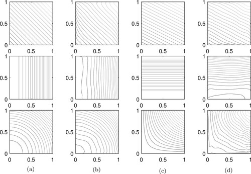
Observe that the number of unknowns is $2(n+1{)}^2=512$, which is exactly the number of IVPs solved every time the Jacobian is needed. However, as it can be seen in Table 5, good quality results are obtained in a fairly small number of iterations (and so Jacobian computations as well). This shows that the proposed strategy is able to produce suitable reconstructions with acceptable computational effort, and so it can be useful in real-world applications.

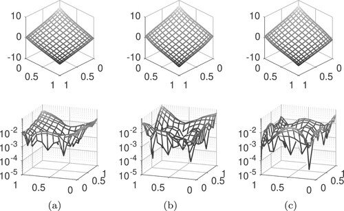
Finally, to assess the quality of recovered conductivities, we solve the forward problem with conductivities determined with LMM as input data and compare the obtained solution T against the considered true function values T (generated via FEM). Results of the comparison as well as absolute value of the errors are displayed in Figure 10. Good fitting between data provided by FEM and approximations given by our strategy is evident. We point out that FEM solutions may contain imprecisions due to discretization and/or numerical treatment, in a way that our solutions could be even better if compared with the exact (yet unavailable) data.

Figure 10. Computed temperature T (above) at time t = 1 using the reconstructions of $k_{11}$ and $k_{22}$ and the absolute value of the error between FEM's T and its approximation (below).

5. Conclusion

We proposed a method for reconstructing orthotropic conductivity combining a solver for the direct problem based on a Chebyshev pseudospectral method and Levenberg–Marquardt method for solving a related non-linear least squares problem. The main feature of the proposed method is that instead of scaling diagonal matrices often used in classical LMM implementations, we use singular regularization matrices. The impact of such a replacement in terms of the quality of the reconstruction was illustrated with numerical experiments. Further, to cope with typical instabilities in inverse reconstruction problems due to noise in the data, we use the Morozov discrepancy principle as stopping rule. Numerical results show a good fit between exact and recovered conductivity at a very low computational cost, and exceptional stability when inverting noisy data due to the use of Morozov's stopping rule. The reason for this is because the method is simple to implement as well as because CPM builds high-order approximations using a rather small set of discretization points, contributing greatly for the reduction of computational effort. Future work includes the extension to simultaneous reconstruction of capacity and conductivity, as well as the LMM convergence analysis under the assumption that scaling matrices are replaced by singular matrices, as made in this paper.

Disclosure statement

No potential conflict of interest was reported by the author(s).

Additional information

Funding

EB was supported by Coordenação de Aperfeiçoamento de Pessoal de Nível Superior (CAPES), Brazil [grant number 88887.178114/2018-00] and Fundação de Amparo à Pesquisa e Inovação do Estado de Santa Catarina (FAPESC), Brazil [grant number 88887.178114/2018-00]. FSVB was supported by Conselho Nacional de Desenvolvimento Científico e Tecnológico (CNPq), Brazil [grant number 308523/2017-2].

References

- Özişik MN. Boundary value problems of heat conduction. Mineola (NY): ITC; 1968.
- Alessandrini G, de Hoop MV, Gaburro R. Uniqueness for the electrostatic inverse boundary value problem with piecewise constant anisotropic conductivities. Inverse Probl. 2017;33(12):125013.
- Astala K, Päivärinta L. Calderón's inverse problem for anisotropic conductivity in the plane. Commun Par Diff Eq. 2005;30(1–2):207–224.
- Gaburro R, Sincich E. Lipschitz stability for the inverse conductivity problem for a conformal class of anisotropic conductivities. Inverse Probl. 2015;31(1):015008.
- Isakov V. Inverse problems for partial differential equations. 2nd ed. Applied Mathematical Sciences. New York (NY): Springer; 2006.
- Alifanov OM. Inverse heat transfer problems. 1st ed. International Series in Heat and Mass Transfer. Berlin: Springer-Verlag; 1994.
- Elayyan A, Isakov V. On uniqueness of recovery of the discontinuous conductivity coefficient of a parabolic equation. SIAM J Math Anal. 1997;28(1):49–59.
- Carrera J, Neuman SP. Estimation of aquifer parameters under transient and steady-state conditions: 2. Uniqueness, stability and solution algorithms. Water Resour Res. 1986;22:211–227.
- Gol'dman NL. Inverse problems with final overdetermination for parabolic equations with unknown coefficients multiplying the highest derivative. Dokl Math. 2011;83:316–320.
- Huntul MJ, Hussein MS, Lesnic D, et al. Reconstruction of an orthotropic thermal conductivity from non-local heat flux measurements. Int J Math Model Numer Optim. 2020;10(1):102–122.
- Lionheart WRB. Conformal uniqueness results in anisotropic electrical impedance imaging. Inverse Probl. 1997;13(1):125–134.
- Mejias MM, Orlande HRB, Özişik MN. Effects of the heating process and body dimensions on the estimation of the thermal conductivity components of orthotropic solids. Inverse Probl Sci Eng. 2003;11(1):75–89.
- Rodrigues FA, Orlande HRB, Mejias MM. Use of a single heated surface for the estimation of thermal conductivity components of orthotropic 3D solids. Inverse Probl Sci Eng. 2004;12(5):501–517.
- Yen RH, Chen CY, Huang CT, et al. Numerical study of anisotropic thermal conductivity fabrics with heating elements. Int J Numer Method Heat Fluid Flow. 2013;23(5):750–771.
- Pasdunkorale J, Turner IW. A second order finite volume technique for simulating transport in anisotropic media. Int J Numer Method Heat Fluid Flow. 2003;13(1):31–56.
- Kohn R, Vogelius M. Determining conductivity by boundary measurements II. Interior results. Commun Pure Appl Math. 1985;38(5):643–667.
- Mera NS, Elliott L, Ingham DB, et al. A comparison of different regularization methods for a Cauchy problem in anisotropic heat conduction. Int J Numer Method Heat Fluid Flow. 2003;13(5):528–546.
- Mera NS, Elliott L, Ingham DB, et al. An iterative BEM for the Cauchy steady state heat conduction problem in an anisotropic medium with unknown thermal conductivity tensor. Inverse Probl Eng. 2000;8(6):579–607.
- Zhou HL, Xiao X, Chen HL, et al. Identification of thermal conductivity for orthotropic FGMs by DT-DRBEM and L-M algorithm. Inverse Probl Sci Eng. 2020;28(2):196–219.
- Mahmood MS, Lesnic D. Identification of conductivity in inhomogeneous orthotropic media. Int J Numer Method Heat Fluid Flow. 2019;29(1):165–183.
- Cao K, Lesnic D, Cola MJ. Determination of thermal conductivity of inhomogeneous orthotropic materials from temperature measurements. Inverse Probl Sci Eng. 2019;27(10):1372–1398.
- Monard F, Rim D. Imaging of isotropic and anisotropic conductivities from power densities in three dimensions. Inverse Probl. 2018;34(7):075005.
- Mustonen L. Numerical study of a parametric parabolic equation and a related inverse boundary value problem. Inverse Probl. 2016;32(10):105008.
- Borggaard J, van Wyk HW. Gradient-based estimation of uncertain parameters for elliptic partial differential equations. Inverse Probl. 2015;31(6):065008.
- Young LC. Orthogonal collocation revisited. Comput Methods Appl Mech Engrg. 2019;345:1033–1076.
- Berntsson F. A spectral method for solving the sideways heat equation. Inverse Probl. 1999;15(4):891–906.
- Ismailov MI, Bazán FSV, Bedin L. Time-dependent perfusion coefficient estimation in a bioheat transfer problem. Comput Phys Commun. 2018;230:50–58.
- Bazán FSV. Chebyshev pseudospectral method for wave equation with absorbing boundary conditions that does not use a first order hyperbolic system. Math Comput Simul. 2010;80(11):2124–2133.
- Bazán FSV, Bedin L, Bozzoli F. New methods for numerical estimation of convective heat transfer coefficient in circular ducts. Int J Therm Sci. 2019;139:387–402.
- Trefethen LN. Spectral methods in MATLAB. Vol. 10. Philadelphia (PA): Society for Industrial and Applied Mathematics; 2000.
- Gottlieb D, Orzag SA. Numerical analysis of spectral methods: theory and applications. Philadelphia (PA): SIAM; 1977.
- Yamashita N, Fukushima M. On the rate of convergence of the Levenberg-Marquardt method. In: Alefeld G, Chen X, editors. Topics in numerical analysis. Vol. 15. Vienna: Springer; 2001. p. 239–249.
- Morozov VA. Regularization methods for solving incorrectly posed problems. 1st ed. New York (NY): Springer-Verlag; 1984.
- Canuto C, Hussaini MY, Quarteroni A. Spectral methods in fluid dynamics. 1st ed. Springer Series in Computational Physics. Berlin: Springer-Verlag; 1988.
- Bernardi C, Maday Y. Approximations spectrales de problèmes methods aux limites elliptiques. 1st ed. Berlin: Springer-Verlag; 1992.
- Crank J, Nicolson P. A practical method for numerical evaluation of solutions of partial differential equations of the heat-conduction type. Math Proc Cambridge Philos Soc. 1947;43(1):50–67.
- Tikhonov AN, Goncharsky AV, Stepanov VV. Numerical methods for the solution of ill-posed problems. 1st ed. Vol. 328. Dordrecht: Springer Science & Business Media; 1995.
- Toint PL. Non-monotone trust region algorithm for nonlinear optimization subject to convex constraints. Math Program. 1997;77(3):69–94.
- Francisco JB, Bazán FSV. Nonmonotone algorithm for minimization on closed sets with application to minimization on Stiffen manifolds. J Comput Appl Math. 2012;236(10):2717–2727.
- Moré JJ. The Levenberg-Marquardt algorithm: implementation and theory. In: Watson GA, editor. Numerical analysis. Lecture Notes in Mathematics; Vol. 630. Berlin: Springer; 1978. p. 105–116.
- Bazán FSV, Cunha MCC, Borges LS. Extension of GKB-FP algorithm to large-scale general-form Tikhonov regularization. Numer Linear Algebra. 2014;21(3):316–339.
- Johnson C. Numerical solution of partial differential equations by the finite element method. 1st ed. Cambridge: Cambridge University Press; 1987.
- Larson MG, Bengzon F. The finite element method: theory, implementation, and applications. 1st ed. Berlin: Springer; 2013; Texts in Computational Science and Engineering.
- Mueller J, Siltanen S. Linear and nonlinear inverse problems with practical applications. Vol. 10. Philadelphia (PA): Society for Industrial and Applied Mathematics; 2012.
- Chávez CE, Atienza FA, Álvarez D. Avoiding the inverse crime in the inverse problem of electrocardiography: estimating the shape and location of cardiac ischemia. In: Computing in cardiology 2013; 2013. p. 687–690.
- Kelley CT. Iterative methods for optimization. Philadelphia (PA): Society for Industrial and Applied Mathematics; 1999.
- Kaltenbacher B, Neubauer A, Scherzer O. Iterative regularization methods for nonlinear ill-posed problems. Radon Series on Computational and Applied Mathematics; Vol. 6. Berlin: De Gruyter; 2008.
- Natterer F. The mathematics of computerized tomography. Stuttgart: Wiley; 1986.