An inverse problem of a simultaneous reconstruction of the dielectric constant and conductivity from experimental backscattering data

Abstract

This report extends our recent progress in tackling a challenging 3D inverse scattering problem governed by the Helmholtz equation. Our target application is to reconstruct dielectric constants, electric conductivities and shapes of front surfaces of objects buried very closely under the ground. These objects mimic explosives, like, e.g. antipersonnel land mines and improvised explosive devices. We solve a coefficient inverse problem with the backscattering data generated by a moving source at a fixed frequency. This scenario has been studied so far by our newly developed convexification method that consists in a new derivation of a boundary value problem for a coupled quasilinear elliptic system. However, in our previous work only the unknown dielectric constants of objects and shapes of their front surfaces were calculated. Unlike this, in the current work performance of our numerical convexification algorithm is verified for the case when the dielectric constants, the electric conductivities and those shapes of objects are unknown. By running several tests with experimentally collected backscattering data, we find that we can accurately image both the dielectric constants and shapes of targets of interests including a challenging case of targets with voids. The computed electrical conductivity serves for reliably distinguishing conductive and non-conductive objects. The global convergence of our numerical procedure is shortly revisited.

Keywords:

• Coefficient inverse problem
• multiple point sources
• experimental data
• Carleman weight
• global convergence
• Fourier series

MSC:

• 78A46
• 65L70
• 65C20

1. Introduction

In this paper, we present an extension of our previous numerical studies of the performance on both computationally simulated [1] and experimental data [2] of our newly developed globally convergent convexification numerical method for a Coefficient Inverse Problem (CIP) for the Helmholtz equation in the 3D case. This new approach has been established so far to solve a 3D CIP with a fixed frequency and the point source moving along an interval of a straight line. Our target application is in the reconstruction of physical properties of explosive-like objects buried closely under the ground, such as antipersonnel land mines and improvised explosive devices (IEDs). There are four (4) important properties of such targets that we are currently interested in:

1. Dielectric constants

2. Locations

3. Shapes of front surfaces

4. Electrical conductivities.

The previous work [3] was concerned with the first two properties for a different set of experimental data and for a different version of the convexification method. In [3], the point source was fixed and the frequency was varied. However, shapes of targets of interests or, at the very least, their front surfaces were not accurately imaged in that scenario. This reveals an advantage of the context considered both in [1,2] and in this paper, compared with the previous studies of the research group of the third author.

As we have seen, the dielectric constants and shapes of front surfaces of the targets with different types of materials and geometries can be recovered via the convexification from our experimentally collected data [2]. Thus this paper is about the recovery of the fourth property, the electrical conductivity, simultaneously with the three above ones. We refer to publications of the research group of Novikov for a variety of CIPs with the data at a single frequency [4–8]. Both statements of those CIPs and methods of their treatments are different from ours. Also, we refer to [9] for a different numerical method for a similar CIP.

A conventional way to solve a CIP is numerically via the minimization of a conventional least squares cost functional; see, e.g. [10–12]. The major problem with this approach, however, is that such a functional is nonconvex and typically suffers from the phenomenon of multiple local minima and ravines. Since any gradient-like method stops at any point of a local minimum, then any convergence result for this method would be valid only if the starting point of iterations would be located in a small neighbourhood of the correct solution. However, it is unclear how to a priori find such a point. In other words, conventional numerical methods for CIPs are locally convergent ones.

Definition 1.1

We call a numerical method for a CIP globally convergent if there is a theorem, which claims that this method delivers at least one point in a sufficiently small neighbourhood of the correct solution without any advanced knowledge of this neighbourhood.

The convexification is a globally convergent numerical method. It works with the most challenging case of data collection: our data are both backscattering and non-overdetermined ones. Given a CIP, we call the data for it non-overdetermined if the number m of free variables in the data equals the number n of free variables in the unknown coefficient, i.e. m = n. If m>n, then the data are overdetermined. In this paper, m = n = 3. The authors are unaware about such numerical methods for the CIPs with the non-overdetermined data at $m=n\ge 2$, which would be based on the minimization of a conventional least squares cost functional and, at the same time, would be globally convergent in terms of the above definition.

The latter is the reason why the third author and his collaborators have been working on the convexification for a number of years; see, e.g. [13–16] for some first publications in this direction. After a certain change of variables, the convexification constructs a weighted cost functional $J_{\lambda }$, where $\lambda \ge 1$ is a parameter. The main element of $J_{\lambda }$ is the presence of the Carleman Weight Function (CWF) in it. This is the function, which participates as a weight in the Carleman estimate for the corresponding partial differential operator. The main theorem then is that, given a convex bounded set $B(d)\subset H$ of an arbitrary diameter d in an appropriate Hilbert space H, one can choose such a set of parameters λ that the functional $J_{\lambda }$ is strictly convex on $B(d).$ This guarantees, of course, the absence of local minima and ravines on $B(d).$ Using that theorem, the global convergence to the correct solution of the gradient projection method on $B(d)$ is established.

The above cited first works on the convexification lacked some theorems justifying the latter global convergence property and, therefore, numerical results in them were not present, except of some first ones in [16]. Fortunately, however, the paper [17] has cleared that global convergence issue, which has resulted in a number of recent publications, where the theory of the convexification is complemented by numerical studies, see, e.g. [1,18–20]. In particular, experimental data are treated by the convexification in [2,3,21]. In [22,23], the second version of the convexification is developed for CIPs for hyperbolic PDEs. Ideas of [22,23] are explored further in [24,25].

In both versions of the convexification, the ideas of the Bukhgeim–Klibanov method play the foundational role. This method is based on Carleman estimates. Initially it was proposed in 1981 only for proofs of uniqueness theorems for multidimensional CIPs; see [26] for the first publication, and a survey of this method can be found in [27].

This paper is organized as follows. In Section 2, we state our CIP. In Section 3, we construct our functional $J_{\lambda }$ and formulate main theoretical results about it, which we took from our recent work [2]. Finally, in Section 4 we present our numerical results.

2. Statement of the inverse problem

Even though the propagation of electromagnetic waves is governed by the Maxwell's equations, we use only the Helmholtz equation in this paper. Indeed, it was demonstrated numerically in the appendix of the paper [28] that this equation describes the propagation of one component of the electric field equally well with the Maxwell's equations. Another confirmation comes from our successful work with experimental data, both in [2,3] and in this paper.

Let $\mathbf{x}=(x,y,z)\in {\mathbb{R}}^3$. Prior to the statement of the inverse problem, we first consider the following time-harmonic Helmholtz wave equation with conductivity: (1) $\mathrm{\Delta }u+({\omega }^2\mu {\epsilon }^{\mathrm{\prime }}\left(\mathbf{x}\right)-\mathrm{i}\omega \mu \sigma \left(\mathbf{x}\right))u=-\delta (\mathbf{x}-{\mathbf{x}}_{\alpha })\mathrm{in}{\mathbb{R}}^3,\mathrm{i}=\sqrt{-1}.$(1) Cf. [29, Section 3.3], the function $u=u(\mathbf{x},\alpha )$ in (1(1) $\mathrm{\Delta }u+({\omega }^2\mu {\epsilon }^{\mathrm{\prime }}\left(\mathbf{x}\right)-\mathrm{i}\omega \mu \sigma \left(\mathbf{x}\right))u=-\delta (\mathbf{x}-{\mathbf{x}}_{\alpha })\mathrm{in}{\mathbb{R}}^3,\mathrm{i}=\sqrt{-1}.$(1) ) can be physically understood as a component of the electric field $E=(E_x,E_y,E_z)$, which corresponds to a single nonzero component of the incident field. In our case, this component is $E_y$ (voltage) which is being incident upon the medium. The backscattering signal of the same component was measured in our experiments. In (1(1) $\mathrm{\Delta }u+({\omega }^2\mu {\epsilon }^{\mathrm{\prime }}\left(\mathbf{x}\right)-\mathrm{i}\omega \mu \sigma \left(\mathbf{x}\right))u=-\delta (\mathbf{x}-{\mathbf{x}}_{\alpha })\mathrm{in}{\mathbb{R}}^3,\mathrm{i}=\sqrt{-1}.$(1) ), ω is the angular frequency ($\mathrm{rad}/\mathrm{m}$), $\mu ,{\epsilon }^{\mathrm{\prime }}(\mathbf{x}),\sigma (\mathbf{x})$ represent respectively the permeability ($\mathrm{H}/\mathrm{m}$), permittivity ($\mathrm{F}/\mathrm{m}$) and (effective) conductivity ($\mathrm{S}/\mathrm{m}$) of the medium. Furthermore, ${\mathbf{x}}_{\alpha }$ is the point source which will be defined below.

Suppose that we only consider non-magnetic targets. Then their relative permeability has to be unity. With ${\epsilon }_0,{\mu }_0$ being the vacuum permittivity and vacuum permeability, respectively, and $k=\omega \sqrt{{\mu }_0{\epsilon }_0}$, (1(1) $\mathrm{\Delta }u+({\omega }^2\mu {\epsilon }^{\mathrm{\prime }}\left(\mathbf{x}\right)-\mathrm{i}\omega \mu \sigma \left(\mathbf{x}\right))u=-\delta (\mathbf{x}-{\mathbf{x}}_{\alpha })\mathrm{in}{\mathbb{R}}^3,\mathrm{i}=\sqrt{-1}.$(1) ) becomes (2) $\mathrm{\Delta }u+(k^2\frac{\mu }{{\mu }_0}\frac{{\epsilon }^{\mathrm{\prime }}}{{\epsilon }_0}-\mathrm{i}k\sqrt{\frac{\mu }{{\mu }_0}}\sqrt{\frac{\mu }{{\epsilon }_0}}\sigma )u=-\delta (\mathbf{x}-{\mathbf{x}}_{\alpha })\mathrm{in}{\mathbb{R}}^3.$(2) In (2(2) $\mathrm{\Delta }u+(k^2\frac{\mu }{{\mu }_0}\frac{{\epsilon }^{\mathrm{\prime }}}{{\epsilon }_0}-\mathrm{i}k\sqrt{\frac{\mu }{{\mu }_0}}\sqrt{\frac{\mu }{{\epsilon }_0}}\sigma )u=-\delta (\mathbf{x}-{\mathbf{x}}_{\alpha })\mathrm{in}{\mathbb{R}}^3.$(2) ), the fraction $\mu /{\epsilon }_0$ is essentially close to the so-called characteristic impedance of free space ${\mu }_0/{\epsilon }_0=:{\eta }_0$, which is approximately 377 (${\mathrm{S}}^{-1}$). Denote $c={\epsilon }^{\mathrm{\prime }}/\epsilon$ as the dielectric constant. We therefore rewrite the Helmholtz equation (2(2) $\mathrm{\Delta }u+(k^2\frac{\mu }{{\mu }_0}\frac{{\epsilon }^{\mathrm{\prime }}}{{\epsilon }_0}-\mathrm{i}k\sqrt{\frac{\mu }{{\mu }_0}}\sqrt{\frac{\mu }{{\epsilon }_0}}\sigma )u=-\delta (\mathbf{x}-{\mathbf{x}}_{\alpha })\mathrm{in}{\mathbb{R}}^3.$(2) ) and impose the Sommerfeld radiation condition: (3) $\begin{array}{rl}& \mathrm{\Delta }u+(k^{2}c-\mathrm{i}k{\eta }_0\sigma )u=-\delta (\mathbf{x}-{\mathbf{x}}_{\alpha })\mathrm{in}{\mathbb{R}}^3,\end{array}$(3) (4) $\begin{array}{rl}& \underset{r\to \mathrm{\infty }}{lim}r({\mathrm{\partial }}_{r}u-\mathrm{i}ku)=0\mathrm{for}r=|\mathbf{x}-{\mathbf{x}}_{\alpha }|,\mathrm{i}=\sqrt{-1}.\end{array}$(4)

We now pose the inverse problem. Consider a rectangular prism $\mathrm{\Omega }=(-R,R)\times (-R,R)\times (-b,b)$ in ${\mathbb{R}}^3$ for numbers R, b>0. This prism is our computational domain of interest. Let $c=c(\mathbf{x})$ and $\sigma =\sigma (\mathbf{x})$ be the spatially distributed dielectric constant and electrical conductivity of the medium, respectively. We assume that these functions are smooth and satisfy the following conditions: (5) $\{\begin{array}{ll}c\left(\mathbf{x}\right)\ge 1& \mathrm{in}\mathrm{\Omega },\\ c\left(\mathbf{x}\right)=1& \mathrm{in}{\mathbb{R}}^3\mathrm{\setminus }\mathrm{\Omega },\end{array}\mathrm{and}\{\begin{array}{ll}\sigma \left(\mathbf{x}\right)\ge 0& \mathrm{in}\mathrm{\Omega },\\ \sigma \left(\mathbf{x}\right)=0& \mathrm{in}{\mathbb{R}}^3\mathrm{\setminus }\mathrm{\Omega }.\end{array}$(5) The second line of (5(5) $\{\begin{array}{ll}c\left(\mathbf{x}\right)\ge 1& \mathrm{in}\mathrm{\Omega },\\ c\left(\mathbf{x}\right)=1& \mathrm{in}{\mathbb{R}}^3\mathrm{\setminus }\mathrm{\Omega },\end{array}\mathrm{and}\{\begin{array}{ll}\sigma \left(\mathbf{x}\right)\ge 0& \mathrm{in}\mathrm{\Omega },\\ \sigma \left(\mathbf{x}\right)=0& \mathrm{in}{\mathbb{R}}^3\mathrm{\setminus }\mathrm{\Omega }.\end{array}$(5) ) means that we are assuming to have vacuum outside of the domain of interest Ω. Let the number d>b and let $a_1<a_2$. We consider the line of sources, (6) $L_{\mathrm{src}}:=\{(\alpha ,0,-d):a_1\le \alpha \le a_2\}.$(6) This line is parallel to the x-axis and is located outside of the closed domain $\overline{\mathrm{\Omega }}$. The distance between $L_{\mathrm{src}}$ and the xy-plane is d, and the length of the line of sources is $(a_2-a_1)$. Using this setting, we arrange for each $\alpha \in [a_1,a_2]$ the point source ${\mathbf{x}}_{\alpha }:=(\alpha ,0,-d)$ located on the straight line $L_{\mathrm{src}}$. We also define the near-field measurement site as the lower side of the prism Ω, $\mathrm{\Gamma }:=\{\mathbf{x}:\left|x\right|,\left|y\right|<R,z=-b\}.$ To this end, we use either α or ${\mathbf{x}}_{\alpha }$ to indicate the dependence of a function/parameter/number on those point sources. We denote by u, $u_i$ and $u_s$ the total wave, incident wave and scattered wave, respectively. Also, we note that $u=u_i+u_s$.

Forward problem

Given the wavenumber k>0 and the functions $c(\mathbf{x}),\sigma (\mathbf{x}),$ the forward problem is to seek the function $u(\mathbf{x},\alpha ){|}_{\mathrm{\Gamma }}$ such that the function $u=u(\mathbf{x},\alpha )$ is the solution of problem (3(3) $\begin{array}{rl}& \mathrm{\Delta }u+(k^{2}c-\mathrm{i}k{\eta }_0\sigma )u=-\delta (\mathbf{x}-{\mathbf{x}}_{\alpha })\mathrm{in}{\mathbb{R}}^3,\end{array}$(3) )–(4(4) $\begin{array}{rl}& \underset{r\to \mathrm{\infty }}{lim}r({\mathrm{\partial }}_{r}u-\mathrm{i}ku)=0\mathrm{for}r=|\mathbf{x}-{\mathbf{x}}_{\alpha }|,\mathrm{i}=\sqrt{-1}.\end{array}$(4) ).

Here, the incident wave is (7) $u_i(\mathbf{x},\alpha )=\frac{\exp \left(\mathrm{i}k|\mathbf{x}-{\mathbf{x}}_{\alpha }|\right)}{4\pi |\mathbf{x}-{\mathbf{x}}_{\alpha }|}.$(7) Moreover, we can deduce that the scattered wave is (8) $u_s(\mathbf{x},\alpha )={\int }_{\mathrm{\Omega }}\frac{\exp \left(\mathrm{i}k|\mathbf{x}-{\mathbf{x}}^{\mathrm{\prime }}|\right)}{4\pi |\mathbf{x}-{\mathbf{x}}^{\mathrm{\prime }}|}[k^2(c\left({\mathbf{x}}^{\mathrm{\prime }}\right)-1)-\mathrm{i}k{\eta }_0\sigma \left({\mathbf{x}}^{\mathrm{\prime }}\right)]u({\mathbf{x}}^{\mathrm{\prime }},\alpha )\mathrm{d}{\mathbf{x}}^{\mathrm{\prime }},\mathbf{x}\in {\mathbb{R}}^3,$(8) since functions c−1 and σ are compactly supported in Ω; see (5(5) $\{\begin{array}{ll}c\left(\mathbf{x}\right)\ge 1& \mathrm{in}\mathrm{\Omega },\\ c\left(\mathbf{x}\right)=1& \mathrm{in}{\mathbb{R}}^3\mathrm{\setminus }\mathrm{\Omega },\end{array}\mathrm{and}\{\begin{array}{ll}\sigma \left(\mathbf{x}\right)\ge 0& \mathrm{in}\mathrm{\Omega },\\ \sigma \left(\mathbf{x}\right)=0& \mathrm{in}{\mathbb{R}}^3\mathrm{\setminus }\mathrm{\Omega }.\end{array}$(5) ). We then combine (7(7) $u_i(\mathbf{x},\alpha )=\frac{\exp \left(\mathrm{i}k|\mathbf{x}-{\mathbf{x}}_{\alpha }|\right)}{4\pi |\mathbf{x}-{\mathbf{x}}_{\alpha }|}.$(7) ) and (8(8) $u_s(\mathbf{x},\alpha )={\int }_{\mathrm{\Omega }}\frac{\exp \left(\mathrm{i}k|\mathbf{x}-{\mathbf{x}}^{\mathrm{\prime }}|\right)}{4\pi |\mathbf{x}-{\mathbf{x}}^{\mathrm{\prime }}|}[k^2(c\left({\mathbf{x}}^{\mathrm{\prime }}\right)-1)-\mathrm{i}k{\eta }_0\sigma \left({\mathbf{x}}^{\mathrm{\prime }}\right)]u({\mathbf{x}}^{\mathrm{\prime }},\alpha )\mathrm{d}{\mathbf{x}}^{\mathrm{\prime }},\mathbf{x}\in {\mathbb{R}}^3,$(8) ) to obtain the Lippmann–Schwinger equation [30]: $\begin{array}{rl}u(\mathbf{x},\alpha )& =u_i(\mathbf{x},\alpha )+{\int }_{\mathrm{\Omega }}\frac{\exp \left(\mathrm{i}k|\mathbf{x}-{\mathbf{x}}^{\mathrm{\prime }}|\right)}{4\pi |\mathbf{x}-{\mathbf{x}}^{\mathrm{\prime }}|}[k^2(c\left({\mathbf{x}}^{\mathrm{\prime }}\right)-1)-\mathrm{i}k{\eta }_0\sigma \left({\mathbf{x}}^{\mathrm{\prime }}\right)]u({\mathbf{x}}^{\mathrm{\prime }},\alpha )\mathrm{d}{\mathbf{x}}^{\mathrm{\prime }},\\ & \mathbf{x}\in {\mathbb{R}}^3.\end{array}$ In fact, we generate our data $u(\mathbf{x},\alpha ){|}_{\mathrm{\Gamma }}$ via solving this equation.

Coefficient Inverse Problem (CIP)

Given k>0, the CIP is to reconstruct the two smooth functions: the dielectric constant $c(\mathbf{x})$ and the conductivity $\sigma (\mathbf{x})$ for $\mathbf{x}\in \mathrm{\Omega }$ satisfying conditions (5(5) $\{\begin{array}{ll}c\left(\mathbf{x}\right)\ge 1& \mathrm{in}\mathrm{\Omega },\\ c\left(\mathbf{x}\right)=1& \mathrm{in}{\mathbb{R}}^3\mathrm{\setminus }\mathrm{\Omega },\end{array}\mathrm{and}\{\begin{array}{ll}\sigma \left(\mathbf{x}\right)\ge 0& \mathrm{in}\mathrm{\Omega },\\ \sigma \left(\mathbf{x}\right)=0& \mathrm{in}{\mathbb{R}}^3\mathrm{\setminus }\mathrm{\Omega }.\end{array}$(5) ) from the boundary measurement $F_0(\mathbf{x},{\mathbf{x}}_{\alpha })$ of the near-field data, (9) $F_0(\mathbf{x},{\mathbf{x}}_{\alpha })=u(\mathbf{x},\alpha )\mathrm{for}\mathbf{x}\in \mathrm{\Gamma },{\mathbf{x}}_{\alpha }\in L_{\mathrm{src}},$(9) where $u(\mathbf{x},\alpha )$ is the total wave associated with the incident wave $u_i$ of (7(7) $u_i(\mathbf{x},\alpha )=\frac{\exp \left(\mathrm{i}k|\mathbf{x}-{\mathbf{x}}_{\alpha }|\right)}{4\pi |\mathbf{x}-{\mathbf{x}}_{\alpha }|}.$(7) ).

Remark 2.1

Although the far-field data are collected in our experimental setup, our CIP is posed for the case of the near-field data. Experimentally measured backscattering far-field data are not convenient to work with since they do not provide a good indication of the location of the target of interest. This is clear from, e.g. Figure 2 (left). The same observation took place in [2] and [31]. Besides, if using the far-field data in the inversion procedure described below, then the computational domain would be very large. The latter would lead to a significant increase of the computational time and would put unnecessary demands on computer's memory. These considerations led the authors of [2,31] to the so-called ‘data propagation procedure’. By getting rid of high spatial frequencies, this procedure essentially delivers a good approximation for both the near-field data $F_0$ in (9(9) $F_0(\mathbf{x},{\mathbf{x}}_{\alpha })=u(\mathbf{x},\alpha )\mathrm{for}\mathbf{x}\in \mathrm{\Gamma },{\mathbf{x}}_{\alpha }\in L_{\mathrm{src}},$(9) ) (i.e. data at the assigned boundary Γ) and the z-derivative of the function $u(\mathbf{x},\alpha )$ on Γ, (10) $F_1(\mathbf{x},{\mathbf{x}}_{\alpha })=u_z(\mathbf{x},\alpha )\mathrm{for}\mathbf{x}\in \mathrm{\Gamma },{\mathbf{x}}_{\alpha }\in L_{\mathrm{src}}.$(10) In our experience, the function $F_0$ is much more informative than the raw far-field: compare, e.g. left and right figures (Figure 2).

Figure 1. A schematic diagram illustrating our experimental configuration. The transmitter is the antenna put in front of the detector placing the far-field measurement site. The backscattering waves hit the antenna before reaching the detectors. This causes a certain noise in the data.

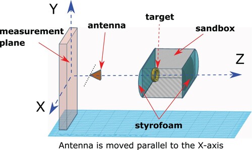
Figure 2. Aluminium cylinder; see Tables 1–2 for further details. (a) and (b) A clear advantage of the data propagation procedure in data preprocessing. (a) Real part of raw and propagated data at $\alpha =0.4$. (b) Imaginary part of raw and propagated data at $\alpha =0.4$. (c) Left: Aluminium cylinder (cf. [2]). Middle: Image of computed dielectric constant. Right: Image of computed conductivity.

Table 1. Chosen wavenumbers, frequencies and wavelength for Examples 1–5.

Example	1	2	3	4	5
k	8.51	6.62	11.43	9.55	8.79
Frequency (GHz)	4.06	3.16	5.45	4.55	4.19
Wavelength (cm)	7.39	9.49	5.50	6.59	7.16

Table 2. True $c_{\mathrm{true}}$, computed $max(c_{\mathrm{comp}})$ dielectric constants and computed conductivity $max({\sigma }_{\mathrm{comp}})$ of Examples 1–5 of experimental data. True values of dielectric constants were taken from: (a) Examples 1, 4, 5: formula (7.2) of [40], (b) Example 2 (clear water) [38], (c) Example 3 [41].

Example	1	2	3	4	5
Object	Metallic cylinder	Water	Wood	Metallic letter ‘A’	Metallic letter ‘O’
$max(c_{\mathrm{comp}})$	28.78	23.18	6.33	16.24	16.22
$c_{\mathrm{true}}$	$[10,30]$	23.8	$[2,6]$	$[10,30]$	$[10,30]$
$max({\sigma }_{\mathrm{comp}})$	2.33	0.94	0.94	1.32	1.66

Remark 2.2

In our experimental setup (cf. Section 4), the inclusions are buried in a sandbox. The sand in this box is our background medium. We know a priori that the dielectric constant and electric conductivity of this sand are $c_{\mathrm{bckgr}}=4$ and ${\sigma }_{\mathrm{bckgr}}=0$ respectively. Although we do not use this information in our numerical method described below, still inclusions in our resulting images are characterized by such values of the parameters $c(\mathbf{x})$ and $\sigma (\mathbf{x})$ that c>4 and $\sigma >0.$ Naturally, a postprocessing procedure is applied to get reasonable values of these parameters inside the inclusions, see Step 3 of section 4.1. The functions $c(\mathbf{x})$ and $\sigma (\mathbf{x})$ in our mathematical statements involve the information of both sand and inclusion. To resolve this issue, in our configuration we measure the raw data twice: when the sandbox is without and with the buried target, respectively. Heuristically, subtraction of these data should be helpful in filtering the information of sand. Our resulting ‘actual’ data (after subtraction) can be applied to the mathematical setting under consideration.

3. A globally convergent numerical method

3.1. A system of coupled quasilinear elliptic PDEs

Since our line of sources $L_{\mathrm{src}}$ is located outside of $\overline{\mathrm{\Omega }}$, we deduce this system from the homogeneous version of Equation (3(3) $\begin{array}{rl}& \mathrm{\Delta }u+(k^{2}c-\mathrm{i}k{\eta }_0\sigma )u=-\delta (\mathbf{x}-{\mathbf{x}}_{\alpha })\mathrm{in}{\mathbb{R}}^3,\end{array}$(3) ) and for each $\alpha \in [a_1,a_2]$ (11) $\mathrm{\Delta }u+(k^{2}c\left(\mathbf{x}\right)-\mathrm{i}k{\eta }_0\sigma \left(\mathbf{x}\right))u=0\mathrm{in}\mathrm{\Omega }.$(11) We set $\log u_i(\mathbf{x},\alpha )=\mathrm{i}k|\mathbf{x}-{\mathbf{x}}_{\alpha }|-\log \left(4\pi |\mathbf{x}-{\mathbf{x}}_{\alpha }|\right),$ which then leads to (12) $\mathrm{\nabla }(\log u_i(\mathbf{x},\alpha ))=\frac{\mathrm{i}k(\mathbf{x}-{\mathbf{x}}_{\alpha })}{|\mathbf{x}-{\mathbf{x}}_{\alpha }|}-\frac{\mathbf{x}-{\mathbf{x}}_{\alpha }}{{|\mathbf{x}-{\mathbf{x}}_{\alpha }|}^2}.$(12) It was established in [32] that, under certain conditions, the function $u(\mathbf{x},\alpha )$ is nowhere nonzero at every point in Ω for sufficiently large values of k, at least in the case when $\sigma (\mathbf{x})\equiv 0.$ This, in turn, has allowed in [1] to uniquely define the function $\log (u(\mathbf{x},\alpha ))$ for those values of k. Thus we assume below that we can uniquely define the function $\log (u(\mathbf{x},\alpha ))$ as in [1]. We note, however, that the condition $u(\mathbf{x},\alpha )\ne 0$ is more important for our derivations below than just defining $\log (u(\mathbf{x},\alpha ))$. This is because only derivatives $\mathrm{\nabla }\log (u(\mathbf{x},\alpha ))=\mathrm{\nabla }u(\mathbf{x},\alpha )/u(\mathbf{x},\alpha )$ and ${\mathrm{\partial }}_{\alpha }\log (u(\mathbf{x},\alpha ))={\mathrm{\partial }}_{\alpha }u(\mathbf{x},\alpha )/u(\mathbf{x},\alpha )$ are involved below and these derivatives are defined uniquely of course.

Denote $v_0(\mathbf{x},\alpha )=u(\mathbf{x},\alpha )/u_i(\mathbf{x},\alpha )$. We define the function $v(\mathbf{x},\alpha )$ as $v(\mathbf{x},\alpha ):=\log \left(v_0(\mathbf{x},\alpha )\right)=\log \left(u(\mathbf{x},\alpha )\right)-\log \left(u_i(\mathbf{x},\alpha )\right)\mathrm{for}\mathbf{x}\in \mathrm{\Omega },\alpha \in [a_1,a_2].$ Hence, one computes that (13) $\mathrm{\nabla }v(\mathbf{x},\alpha )=\frac{\mathrm{\nabla }{v}_0(\mathbf{x},\alpha )}{v_0(\mathbf{x},\alpha )},\mathrm{\Delta }v(\mathbf{x},\alpha )=\frac{\mathrm{\Delta }{v}_0(\mathbf{x},\alpha )}{v_0(\mathbf{x},\alpha )}-{\left(\frac{\mathrm{\nabla }{v}_0(\mathbf{x},\alpha )}{v_0(\mathbf{x},\alpha )}\right)}^2.$(13) Note that $u_i(\mathbf{x},\alpha )$ is the fundamental solution of Equation (11(11) $\mathrm{\Delta }u+(k^{2}c\left(\mathbf{x}\right)-\mathrm{i}k{\eta }_0\sigma \left(\mathbf{x}\right))u=0\mathrm{in}\mathrm{\Omega }.$(11) ) when $c\equiv 1$ and $\sigma \equiv 0$. We have (14) $\mathrm{\Delta }u(\mathbf{x},\alpha )=u_i(\mathbf{x},\alpha )\mathrm{\Delta }{v}_0(\mathbf{x},\alpha )+2\mathrm{\nabla }{u}_i(\mathbf{x},\alpha )\cdot \mathrm{\nabla }{v}_0(\mathbf{x},\alpha )-v_0(\mathbf{x},\alpha )k^2{u}_i(\mathbf{x},\alpha ).$(14) Thus it follows from (11(11) $\mathrm{\Delta }u+(k^{2}c\left(\mathbf{x}\right)-\mathrm{i}k{\eta }_0\sigma \left(\mathbf{x}\right))u=0\mathrm{in}\mathrm{\Omega }.$(11) ) and (14(14) $\mathrm{\Delta }u(\mathbf{x},\alpha )=u_i(\mathbf{x},\alpha )\mathrm{\Delta }{v}_0(\mathbf{x},\alpha )+2\mathrm{\nabla }{u}_i(\mathbf{x},\alpha )\cdot \mathrm{\nabla }{v}_0(\mathbf{x},\alpha )-v_0(\mathbf{x},\alpha )k^2{u}_i(\mathbf{x},\alpha ).$(14) ) that $\begin{array}{rl}& u_i(\mathbf{x},\alpha )\mathrm{\Delta }{v}_0(\mathbf{x},\alpha )+2\mathrm{\nabla }{u}_i(\mathbf{x},\alpha )\cdot \mathrm{\nabla }{v}_0(\mathbf{x},\alpha )\\ & =-[k^2(c\left(\mathbf{x}\right)-1)-\mathrm{i}k\sigma \left(\mathbf{x}\right)]v_0(\mathbf{x},\alpha )u_i(\mathbf{x},\alpha ).\end{array}$ Therefore, combining (11(11) $\mathrm{\Delta }u+(k^{2}c\left(\mathbf{x}\right)-\mathrm{i}k{\eta }_0\sigma \left(\mathbf{x}\right))u=0\mathrm{in}\mathrm{\Omega }.$(11) )–(13(13) $\mathrm{\nabla }v(\mathbf{x},\alpha )=\frac{\mathrm{\nabla }{v}_0(\mathbf{x},\alpha )}{v_0(\mathbf{x},\alpha )},\mathrm{\Delta }v(\mathbf{x},\alpha )=\frac{\mathrm{\Delta }{v}_0(\mathbf{x},\alpha )}{v_0(\mathbf{x},\alpha )}-{\left(\frac{\mathrm{\nabla }{v}_0(\mathbf{x},\alpha )}{v_0(\mathbf{x},\alpha )}\right)}^2.$(13) ) we derive the equation for v, (15) $\mathrm{\Delta }v+{\left(\mathrm{\nabla }v\right)}^2+2\mathrm{\nabla }v\cdot \mathrm{\nabla }(\log \left(u_i(\mathbf{x},\alpha )\right))=-[k^2(c\left(\mathbf{x}\right)-1)-\mathrm{i}k\sigma \left(\mathbf{x}\right)]\mathrm{for}\mathbf{x}\in \mathrm{\Omega }.$(15) We now differentiate (15(15) $\mathrm{\Delta }v+{\left(\mathrm{\nabla }v\right)}^2+2\mathrm{\nabla }v\cdot \mathrm{\nabla }(\log \left(u_i(\mathbf{x},\alpha )\right))=-[k^2(c\left(\mathbf{x}\right)-1)-\mathrm{i}k\sigma \left(\mathbf{x}\right)]\mathrm{for}\mathbf{x}\in \mathrm{\Omega }.$(15) ) with respect to α and use (12(12) $\mathrm{\nabla }(\log u_i(\mathbf{x},\alpha ))=\frac{\mathrm{i}k(\mathbf{x}-{\mathbf{x}}_{\alpha })}{|\mathbf{x}-{\mathbf{x}}_{\alpha }|}-\frac{\mathbf{x}-{\mathbf{x}}_{\alpha }}{{|\mathbf{x}-{\mathbf{x}}_{\alpha }|}^2}.$(12) ) to obtain the following third-order PDE: (16) $\mathrm{\Delta }{\mathrm{\partial }}_{\alpha }v+2\mathrm{\nabla }v\cdot \mathrm{\nabla }{\mathrm{\partial }}_{\alpha }v+2\mathrm{\nabla }{\mathrm{\partial }}_{\alpha }v\cdot {\tilde{\mathbf{x}}}_{\alpha }+2{\hat{\mathbf{x}}}_{\alpha }\cdot \mathrm{\nabla }v=0\mathrm{for}\mathbf{x}\in \mathbf{\Omega },$(16) where, for $\mathbf{x}-{\mathbf{x}}_{\alpha }=(x-\alpha ,y,z+d)\in {\mathbb{R}}^3,$ $\begin{array}{rl}{\tilde{\mathbf{x}}}_{\alpha }& =\frac{\mathrm{i}k(\mathbf{x}-{\mathbf{x}}_{\alpha })}{|\mathbf{x}-{\mathbf{x}}_{\alpha }|}-\frac{\mathbf{x}-{\mathbf{x}}_{\alpha }}{{|\mathbf{x}-{\mathbf{x}}_{\alpha }|}^2},\\ {\hat{\mathbf{x}}}_{\alpha }& =\frac{\mathrm{i}k}{{|\mathbf{x}-{\mathbf{x}}_{\alpha }|}^3}(-y^2-{(z+d)}^2,(x-\alpha )y,(x-\alpha )z)\\ & -\frac{1}{{|\mathbf{x}-{\mathbf{x}}_{\alpha }|}^4}({(x-\alpha )}^2-y^2-{(z+d)}^2,2(x-\alpha )y,2(x-\alpha )z).\end{array}$

Remark 3.1

It is obvious that if the function $v(\mathbf{x},\alpha )$ is known, then we can immediately find the target coefficients $c(\mathbf{x})$ and $\sigma (\mathbf{x})$ by taking the real and imaginary parts of the left-hand side of (15(15) $\mathrm{\Delta }v+{\left(\mathrm{\nabla }v\right)}^2+2\mathrm{\nabla }v\cdot \mathrm{\nabla }(\log \left(u_i(\mathbf{x},\alpha )\right))=-[k^2(c\left(\mathbf{x}\right)-1)-\mathrm{i}k\sigma \left(\mathbf{x}\right)]\mathrm{for}\mathbf{x}\in \mathrm{\Omega }.$(15) ). In order to get rid of the presence of those unknowns in (15(15) $\mathrm{\Delta }v+{\left(\mathrm{\nabla }v\right)}^2+2\mathrm{\nabla }v\cdot \mathrm{\nabla }(\log \left(u_i(\mathbf{x},\alpha )\right))=-[k^2(c\left(\mathbf{x}\right)-1)-\mathrm{i}k\sigma \left(\mathbf{x}\right)]\mathrm{for}\mathbf{x}\in \mathrm{\Omega }.$(15) ), we take advantage of the moving point source via the differentiation with respect to α. This leads to solving the nonlinear third order PDE (16(16) $\mathrm{\Delta }{\mathrm{\partial }}_{\alpha }v+2\mathrm{\nabla }v\cdot \mathrm{\nabla }{\mathrm{\partial }}_{\alpha }v+2\mathrm{\nabla }{\mathrm{\partial }}_{\alpha }v\cdot {\tilde{\mathbf{x}}}_{\alpha }+2{\hat{\mathbf{x}}}_{\alpha }\cdot \mathrm{\nabla }v=0\mathrm{for}\mathbf{x}\in \mathbf{\Omega },$(16) ), which is not an easy task. To overcome this, we apply the Fourier series approach using a special orthonormal basis with respect to α.

For $\alpha \in (a_1,a_2)$, let $\{{\mathrm{\Psi }}_n(\alpha ){\}}_{n=0}^{\mathrm{\infty }}$ be the special orthonormal basis in $L^2(a_1,a_2)$, which was first proposed in [33]. Herewith, the construction of this basis is shortly revisited. For each $n\in \mathbb{N}$, let ${\phi }_n(\alpha )={\alpha }^n{e}^{\alpha }$ for $\alpha \in [a_1,a_2]$. The set $\{{\phi }_n(\alpha ){\}}_{n=0}^{\mathrm{\infty }}$ is linearly independent and complete in $L^2(a_1,a_2)$. Using the Gram–Schmidt orthonormalization procedure, we can obtain the orthonormal basis $\{{\mathrm{\Psi }}_n(\alpha ){\}}_{n=0}^{\mathrm{\infty }}$ in $L^2(a_1,a_2)$, which possesses the following special properties:

• ${\mathrm{\Psi }}_n\in C^{\mathrm{\infty }}[a_1,a_2]$ for all $n\in \mathbb{N}$;

• Let $s_{m,n}=⟨{\mathrm{\Psi }}_n^{\mathrm{\prime }},{\mathrm{\Psi }}_m⟩$, where $⟨\cdot ,\cdot ⟩$ denotes the scalar product in $L^2(a_1,a_2)$. Then the square matrix $S_N=(s_{m,n}{)}_{m,n=0}^{N-1}$ for $N\in \mathbb{N}$ is invertible with $s_{m,n}=1$ if m = n and $s_{m,n}=0$ if n<m.

We note that in the cases of both classical orthonormal polynomials and the basis of trigonometric functions, the first term ${\mathrm{\Psi }}_0$ is a constant, which implies ${\mathrm{\Psi }}_0^{\mathrm{\prime }}\equiv 0$ and $s_{m,0}=0.$ This means that the matrix $S_N$ is not invertible for neither of these cases. Meanwhile, our matrix $S_N$ is an upper diagonal matrix with $det(S_N)=1$. On the other hand, the special second property allows us to reduce the third-order PDE (16(16) $\mathrm{\Delta }{\mathrm{\partial }}_{\alpha }v+2\mathrm{\nabla }v\cdot \mathrm{\nabla }{\mathrm{\partial }}_{\alpha }v+2\mathrm{\nabla }{\mathrm{\partial }}_{\alpha }v\cdot {\tilde{\mathbf{x}}}_{\alpha }+2{\hat{\mathbf{x}}}_{\alpha }\cdot \mathrm{\nabla }v=0\mathrm{for}\mathbf{x}\in \mathbf{\Omega },$(16) ) to a system of coupled elliptic PDEs.

Given $N\in \mathbb{N}$, we consider the following truncated Fourier series for v: (17) $v(\mathbf{x},\alpha )=\sum _{n=0}^{N-1}⟨v(\mathbf{x},\cdot ),{\mathrm{\Psi }}_n(\cdot )⟩{\mathrm{\Psi }}_n\left(\alpha \right)\mathrm{for}\mathbf{x}\in \mathrm{\Omega },\alpha \in [a_1,a_2].$(17) As in [1,2], we substitute (17(17) $v(\mathbf{x},\alpha )=\sum _{n=0}^{N-1}⟨v(\mathbf{x},\cdot ),{\mathrm{\Psi }}_n(\cdot )⟩{\mathrm{\Psi }}_n\left(\alpha \right)\mathrm{for}\mathbf{x}\in \mathrm{\Omega },\alpha \in [a_1,a_2].$(17) ) into (16(16) $\mathrm{\Delta }{\mathrm{\partial }}_{\alpha }v+2\mathrm{\nabla }v\cdot \mathrm{\nabla }{\mathrm{\partial }}_{\alpha }v+2\mathrm{\nabla }{\mathrm{\partial }}_{\alpha }v\cdot {\tilde{\mathbf{x}}}_{\alpha }+2{\hat{\mathbf{x}}}_{\alpha }\cdot \mathrm{\nabla }v=0\mathrm{for}\mathbf{x}\in \mathbf{\Omega },$(16) ), multiplying both sides of the resulting equation by ${\mathrm{\Psi }}_m(\alpha )$ for $0\le m\le N-1$ and then taking the integration with respect to α, we obtain the following system of coupled elliptic equations: (18) $\begin{array}{rl}& \mathrm{\Delta }V\left(\mathbf{x}\right)+K\left(\mathrm{\nabla }V\left(\mathbf{x}\right)\right)=0\mathrm{for}\mathbf{x}\in \mathrm{\Omega },\end{array}$(18) (19) $\begin{array}{rl}& {\mathrm{\partial }}_{\nu }V\left(\mathbf{x}\right)=0\mathrm{for}\mathbf{x}\in \mathrm{\partial }\mathrm{\Omega }\mathrm{\setminus }\mathrm{\Gamma },\end{array}$(19) (20) $\begin{array}{rl}& V\left(\mathbf{x}\right)={\psi }_0\left(\mathbf{x}\right),V_z\left(\mathbf{x}\right)={\psi }_1\left(\mathbf{x}\right)\mathrm{for}\mathbf{x}\in \mathrm{\Gamma },\end{array}$(20) where $\nu =\nu (\mathbf{x})$ is the outward looking normal vector on $\mathrm{\partial }\mathrm{\Omega }\mathrm{\setminus }\mathrm{\Gamma }.$ Here, $V(\mathbf{x})\in {\mathbb{R}}^N$ is the unknown vector function given by (21) $V\left(\mathbf{x}\right)={\left(\begin{array}{cccc}{v}_0\left(\mathbf{x}\right)& v_1\left(\mathbf{x}\right)& \cdots & v_{N-1}\left(\mathbf{x}\right)\end{array}\right)}^T.$(21) Boundary conditions (20(20) $\begin{array}{rl}& V\left(\mathbf{x}\right)={\psi }_0\left(\mathbf{x}\right),V_z\left(\mathbf{x}\right)={\psi }_1\left(\mathbf{x}\right)\mathrm{for}\mathbf{x}\in \mathrm{\Gamma },\end{array}$(20) ) are Cauchy data and are overdetermined ones. A Lipschitz stability estimate for problem (18(18) $\begin{array}{rl}& \mathrm{\Delta }V\left(\mathbf{x}\right)+K\left(\mathrm{\nabla }V\left(\mathbf{x}\right)\right)=0\mathrm{for}\mathbf{x}\in \mathrm{\Omega },\end{array}$(18) )–(20(20) $\begin{array}{rl}& V\left(\mathbf{x}\right)={\psi }_0\left(\mathbf{x}\right),V_z\left(\mathbf{x}\right)={\psi }_1\left(\mathbf{x}\right)\mathrm{for}\mathbf{x}\in \mathrm{\Gamma },\end{array}$(20) ) is obtained in [1] using a Carleman estimate with the same CWF as we work with below.

In PDE (18(18) $\begin{array}{rl}& \mathrm{\Delta }V\left(\mathbf{x}\right)+K\left(\mathrm{\nabla }V\left(\mathbf{x}\right)\right)=0\mathrm{for}\mathbf{x}\in \mathrm{\Omega },\end{array}$(18) ), we denote $K(\mathrm{\nabla }V(\mathbf{x}))=S_N^{-1}f(\mathrm{\nabla }V(\mathbf{x}))$, where $f=((f_m{)}_{m=0}^{N-1}{)}^T\in {\mathbb{R}}^N$ is quadratic with respect to the first derivative of components of $V(\mathbf{x})$, (22) $\begin{array}{rl}{f}_m\left(\mathrm{\nabla }V\left(\mathbf{x}\right)\right)& =2\sum _{n,l=0}^{N-1}\mathrm{\nabla }{v}_n\left(\mathbf{x}\right)\cdot \mathrm{\nabla }{v}_l\left(\mathbf{x}\right){\int }_{a_1}^{a_2}{\mathrm{\Psi }}_m\left(\alpha \right){\mathrm{\Psi }}_n\left(\alpha \right){\mathrm{\Psi }}_l^{\mathrm{\prime }}\left(\alpha \right)\mathrm{d}\alpha \\ & +2\sum _{n=0}^{N-1}{\int }_{a_1}^{a_2}{\mathrm{\Psi }}_m\left(\alpha \right){\mathrm{\Psi }}_n^{\mathrm{\prime }}\left(\alpha \right)\mathrm{\nabla }{v}_n\left(\mathbf{x}\right)\cdot {\tilde{\mathbf{x}}}_{\alpha }\mathrm{d}\alpha \\ & +2\sum _{n=0}^{N-1}{\int }_{a_1}^{a_2}{\mathrm{\Psi }}_m\left(\alpha \right){\mathrm{\Psi }}_n\left(\alpha \right){\hat{\mathbf{x}}}_{\alpha }\cdot \mathrm{\nabla }{v}_n\left(\mathbf{x}\right)\mathrm{d}\alpha .\end{array}$(22)

Remark 3.2

In (20(20) $\begin{array}{rl}& V\left(\mathbf{x}\right)={\psi }_0\left(\mathbf{x}\right),V_z\left(\mathbf{x}\right)={\psi }_1\left(\mathbf{x}\right)\mathrm{for}\mathbf{x}\in \mathrm{\Gamma },\end{array}$(20) ), the boundary value ${\psi }_0$ at Γ is a direct application of the expansion (17(17) $v(\mathbf{x},\alpha )=\sum _{n=0}^{N-1}⟨v(\mathbf{x},\cdot ),{\mathrm{\Psi }}_n(\cdot )⟩{\mathrm{\Psi }}_n\left(\alpha \right)\mathrm{for}\mathbf{x}\in \mathrm{\Omega },\alpha \in [a_1,a_2].$(17) ) to the near field data (9(9) $F_0(\mathbf{x},{\mathbf{x}}_{\alpha })=u(\mathbf{x},\alpha )\mathrm{for}\mathbf{x}\in \mathrm{\Gamma },{\mathbf{x}}_{\alpha }\in L_{\mathrm{src}},$(9) ). As mentioned in Remark 2.1, using the data propagation technique will result in an approximation of the z -derivative $F_1$ of the function  u at Γ, see (10(10) $F_1(\mathbf{x},{\mathbf{x}}_{\alpha })=u_z(\mathbf{x},\alpha )\mathrm{for}\mathbf{x}\in \mathrm{\Gamma },{\mathbf{x}}_{\alpha }\in L_{\mathrm{src}}.$(10) ). The function $F_1$ generates the Neumann boundary condition ${\psi }_1$ in (20(20) $\begin{array}{rl}& V\left(\mathbf{x}\right)={\psi }_0\left(\mathbf{x}\right),V_z\left(\mathbf{x}\right)={\psi }_1\left(\mathbf{x}\right)\mathrm{for}\mathbf{x}\in \mathrm{\Gamma },\end{array}$(20) ) at Γ. It is shown in [2] that the zero Neumann boundary condition (19(19) $\begin{array}{rl}& {\mathrm{\partial }}_{\nu }V\left(\mathbf{x}\right)=0\mathrm{for}\mathbf{x}\in \mathrm{\partial }\mathrm{\Omega }\mathrm{\setminus }\mathrm{\Gamma },\end{array}$(19) ) at $\mathrm{\partial }\mathrm{\Omega }\mathrm{\setminus }\mathrm{\Gamma }$ follows from an approximation of the radiation condition (4(4) $\begin{array}{rl}& \underset{r\to \mathrm{\infty }}{lim}r({\mathrm{\partial }}_{r}u-\mathrm{i}ku)=0\mathrm{for}r=|\mathbf{x}-{\mathbf{x}}_{\alpha }|,\mathrm{i}=\sqrt{-1}.\end{array}$(4) ).

Remark 3.3

From now on we work only within the framework of an approximate mathematical model. This means that we fix the number N of Fourier harmonics in the truncated Fourier series (17(17) $v(\mathbf{x},\alpha )=\sum _{n=0}^{N-1}⟨v(\mathbf{x},\cdot ),{\mathrm{\Psi }}_n(\cdot )⟩{\mathrm{\Psi }}_n\left(\alpha \right)\mathrm{for}\mathbf{x}\in \mathrm{\Omega },\alpha \in [a_1,a_2].$(17) ) and ignore the residual in (18(18) $\begin{array}{rl}& \mathrm{\Delta }V\left(\mathbf{x}\right)+K\left(\mathrm{\nabla }V\left(\mathbf{x}\right)\right)=0\mathrm{for}\mathbf{x}\in \mathrm{\Omega },\end{array}$(18) ). Furthermore, we cannot prove convergence of our method at $N\to \mathrm{\infty }$ since such a proof is an extremely challenging problem. We refer to [1] for a detailed discussion of this issue. We also note that similar approximate mathematical models without proofs of convergence at $N\to \mathrm{\infty }$ are actually used quite often in the field of inverse problems. In this regard, we refer to [4–8,34,35].

3.2. Weighted cost functional in partial finite differences

We set (23) $L\left(V\right)\left(\mathbf{x}\right)=\mathrm{\Delta }V\left(\mathbf{x}\right)+K\left(\mathrm{\nabla }V\left(\mathbf{x}\right)\right).$(23) Let the numbers $\theta >b$ and $\lambda \ge 1$. We define our CWF as (24) ${\mu }_{\lambda }\left(z\right)=\exp \left(2\lambda {(z-\theta )}^2\right)\mathrm{for}z\in [-b,b].$(24) The choice $\theta >b$ is based on the fact that the gradient of the CWF should not vanish in the closed domain $\overline{\mathrm{\Omega }}$. Our CWF is decreasing for $z\in (-b,b)$ and $\underset{z\in [-b,b]}{max}{\mu }_{\lambda }\left(z\right)={\mu }_{\lambda }(-b)={\mathrm{e}}^{2\lambda {(b+\theta )}^2},\underset{z\in [-b,b]}{min}{\mu }_{\lambda }\left(z\right)={\mu }_{\lambda }\left(b\right)={\mathrm{e}}^{2\lambda {(b-\theta )}^2}.$ Therefore, the CWF (24(24) ${\mu }_{\lambda }\left(z\right)=\exp \left(2\lambda {(z-\theta )}^2\right)\mathrm{for}z\in [-b,b].$(24) ) attains its maximal value on the site Γ, and it attains its minimal value on the opposite side. By this way, it ‘maximizes’ the influence of the measured boundary data at z = −b. Furthermore, the notion behind this use of the CWF is to ‘convexify’ the cost functional globally and, especially, to control the nonlinear term $K(\mathrm{\nabla }V(\mathbf{x}))$ in (18(18) $\begin{array}{rl}& \mathrm{\Delta }V\left(\mathbf{x}\right)+K\left(\mathrm{\nabla }V\left(\mathbf{x}\right)\right)=0\mathrm{for}\mathbf{x}\in \mathrm{\Omega },\end{array}$(18) ).

3.2.1. Abstract setting and notation

While the convergence analysis in [1] was done for the case when derivatives in (18(18) $\begin{array}{rl}& \mathrm{\Delta }V\left(\mathbf{x}\right)+K\left(\mathrm{\nabla }V\left(\mathbf{x}\right)\right)=0\mathrm{for}\mathbf{x}\in \mathrm{\Omega },\end{array}$(18) )–(20(20) $\begin{array}{rl}& V\left(\mathbf{x}\right)={\psi }_0\left(\mathbf{x}\right),V_z\left(\mathbf{x}\right)={\psi }_1\left(\mathbf{x}\right)\mathrm{for}\mathbf{x}\in \mathrm{\Gamma },\end{array}$(20) ), (23(23) $L\left(V\right)\left(\mathbf{x}\right)=\mathrm{\Delta }V\left(\mathbf{x}\right)+K\left(\mathrm{\nabla }V\left(\mathbf{x}\right)\right).$(23) )) are considered in their regular continuous setting, in [2], so as in the current paper, we consider the convergence analysis for the case when (18(18) $\begin{array}{rl}& \mathrm{\Delta }V\left(\mathbf{x}\right)+K\left(\mathrm{\nabla }V\left(\mathbf{x}\right)\right)=0\mathrm{for}\mathbf{x}\in \mathrm{\Omega },\end{array}$(18) )–(20(20) $\begin{array}{rl}& V\left(\mathbf{x}\right)={\psi }_0\left(\mathbf{x}\right),V_z\left(\mathbf{x}\right)={\psi }_1\left(\mathbf{x}\right)\mathrm{for}\mathbf{x}\in \mathrm{\Gamma },\end{array}$(20) ), (23(23) $L\left(V\right)\left(\mathbf{x}\right)=\mathrm{\Delta }V\left(\mathbf{x}\right)+K\left(\mathrm{\nabla }V\left(\mathbf{x}\right)\right).$(23) ) are written via ‘partial finite differences’. This means that we use finite differences with respect the variables x, y and keep the standard derivatives with respect to z. It was pointed out in [2] that an important reason of doing so is that partial finite differences allow us not to use the penalty regularization term in our weighted cost functional, which is convenient for computations. When doing so, we use the same grid step size h in x and y directions and do not allow h to tend to zero. Note that it is impractical to use too small grid step sizes in computations. Consider two partitions of the interval $[-R,R],$ $\begin{array}{rl}& -R=x_0<x_1<\dots <x_{Z_h-1}<x_{Z_h}=R,x_p-x_{p-1}=h,\\ & -R=y_0<y_1<\dots <y_{Z_h-1}<y_{Z_h}=R,y_q-y_{q-1}=h.\end{array}$ Then, for any N-dimensional vector function $u(\mathbf{x})$, we denote by $u_{p,q}^h(z)=u(x_p,y_q,z)$ the corresponding semi-discrete function defined at grid points $\{(x_p,y_q){\}}_{p,q=0}^{Z_h}$. Thus the interior grid points are $\{(x_p,y_q){\}}_{p,q=1}^{Z_h-1}$. Denote $\begin{array}{rl}& {\mathrm{\Omega }}_h=\{(x_p,y_q,z):{\left\{(x_p,y_q)\right\}}_{p,q=0}^{Z_h-1}\subset [-R,R]\times [-R,R],z\in (-b,b)\},\\ & {\mathrm{\Gamma }}_h=\{(x_p,y_q,-b):{\left\{(x_p,y_q)\right\}}_{p,q=0}^{Z_h-1}\subset [-R,R]\times [-R,R]\}.\end{array}$ Henceforth, the corresponding Laplace operator in partial finite differences is given by ${\mathrm{\Delta }}^h{u}^h=u_{zz}^h+u_{xx}^h+u_{yy}^h$, where, for interior points of ${\mathrm{\Omega }}_h$, we use $u_{xx}^h=h^{-2}(u_{p+1,q}^h\left(z\right)-2u_{p,q}^h\left(z\right)+u_{p-1,q}^h\left(z\right)),p,q\in [1,Z_h-1]$ and similarly for $u_{yy}^h$. We define for interior points ${\mathrm{\nabla }}^h{u}_{p,q}(z)=({\mathrm{\partial }}_x^h{u}_{p,q}(z),{\mathrm{\partial }}_y^h{u}_{p,q}(z),{\mathrm{\partial }}_z{u}_{p,q}^h(z))$. Here, ${\mathrm{\partial }}_x^h{u}_{p,q}^h(z)=(2h{)}^{-1}(u_{p+1,q}^h(z)-u_{p-1,q}^h(z))$. Hence, the differential operator (23(23) $L\left(V\right)\left(\mathbf{x}\right)=\mathrm{\Delta }V\left(\mathbf{x}\right)+K\left(\mathrm{\nabla }V\left(\mathbf{x}\right)\right).$(23) ) has the following form in the partial finite differences: (25) $L^h\left(V^h\left(z\right)\right)={\mathrm{\Delta }}^h{V}^h\left(z\right)+K\left({\mathrm{\nabla }}^h{V}^h\left(z\right)\right).$(25) To simplify the presentation, we consider any N–D complex valued function $W=\mathrm{Re}W+$i$\mathrm{Im}W$ as the $2N$–D vector function with real valued components $(\mathrm{Re}W,\mathrm{Im}W):=(W_1,W_2):=W\in {\mathbb{R}}^{2N}$.

Denote $w^h(z)$ the vector function $w^h(z)=\{w_{p,q}(z){\}}_{p,q=0}^{Z_h},$ where $w_{p,q}^h(z)=w(x_p,y_q,z).$ Next, we consider $2N-$D vector functions (26) $W^h\left(z\right)={(w_{0,1}^h\left(z\right),w_{0,2}^h\left(z\right),w_{1,1}^h\left(z\right),w_{1,2}^h\left(z\right),\dots ,w_{N-1,1}^h\left(z\right),w_{N-1,2}^h\left(z\right))}^T,$(26) where $w_{s,1}^h(z)=\mathrm{Re}{w}_s^h(z)$ and $w_{s,2}^h(z)=\mathrm{Im}{w}_s^h(z).$ In notations of spaces below, the subscript ‘$2N$’ means that this space consists of such vector functions. As in [2], we consider the Hilbert spaces $H_{2N}^{2,h}=H_{2N}^{2,h}({\mathrm{\Omega }}_h)$ and $L_{2N}^{2,h}=L_{2N}^{2,h}({\mathrm{\Omega }}_h)$ of semi-discrete real valued functions: $\begin{array}{rl}{H}_{2N}^{2,h}& =\{W^h\left(z\right):{\Vert W^h\Vert }_{H_{2N}^{2,h}}^2:=\sum _{s=1}^{N-1}\sum _{j=1}^2\sum _{p,q=1}^{Z_h-1}\sum _{m=0}^2{h}^2{\int }_{-b}^b{\left|{\mathrm{\partial }}_z^m{w}_{s,j,p,q}^h\left(z\right)\right|}^2\mathrm{d}z<\mathrm{\infty }\},\\ L_{2N}^{2,h}& =\{w^h\left(z\right):{\Vert w^h\Vert }_{L_{2N}^{2,h}}^2:=\sum _{s=1}^{N-1}\sum _{j=1}^2\sum _{p,q=1}^{Z_h-1}{h}^2{\int }_{-b}^b{\left|w_{s,j,p,q}^h\left(z\right)\right|}^2\mathrm{d}z<\mathrm{\infty }\}.\end{array}$ Denote $(\cdot ,\cdot )$ the scalar product in the space $H_{2N}^{2,h}({\mathrm{\Omega }}_h)$. The subspace $H_{2N,0}^{2,h}\subset H_{2N}^{2,h}$ is defined as $H_{2N,0}^{2,h}=\{w^h\left(z\right)\in H_{2N}^{2,h}:{{\mathrm{\nabla }}^h{w}_{p,q}^h\left(z\right)|}_{\mathrm{\partial }{\mathrm{\Omega }}_h\mathrm{\setminus }{\mathrm{\Gamma }}_h}\cdot \nu =0,{w_{p,q}^h\left(z\right)|}_{{\mathrm{\Gamma }}_h}={{\mathrm{\partial }}_z{w}_{p,q}^h\left(z\right)|}_{{\mathrm{\Gamma }}_h}=0\}.$ Let $h_0>0$ be a fixed positive number. We assume below that (27) $h\ge h_0>0.$(27) For an arbitrary M>0 let the sets $B(M)\subset H_{2N}^{2,h}({\mathrm{\Omega }}_h)$ and $B_0(M)\subset H_{2N,0}^{2,h}$ be (28) $\begin{array}{rl}& B\left(M\right):=\{V^h\in H_{2N}^{2,h}:{\Vert V^h\Vert }_{H_{2N}^{2,h}}<M,{{\mathrm{\nabla }}^h{V}^h|}_{\mathrm{\partial }{\mathrm{\Omega }}_h\mathrm{\setminus }{\mathrm{\Gamma }}_h}\\ & \cdot \nu =0,{V^h|}_{{\mathrm{\Gamma }}_h}={\psi }_0^h,{{\mathrm{\partial }}_z{V}^h|}_{{\mathrm{\Gamma }}_h}={\psi }_1^h\},\end{array}$(28) (29) $\begin{array}{rl}& B_0\left(M\right)=\{V^h\in H_{2N,0}^{2,h}:{\Vert V^h\Vert }_{H_{2N}^{2,h}}<M\}.\end{array}$(29)

3.2.2. Minimization problem and convergence results

Under the partial finite differences setting, we seek an approximate solution of system (18(18) $\begin{array}{rl}& \mathrm{\Delta }V\left(\mathbf{x}\right)+K\left(\mathrm{\nabla }V\left(\mathbf{x}\right)\right)=0\mathrm{for}\mathbf{x}\in \mathrm{\Omega },\end{array}$(18) )–(20(20) $\begin{array}{rl}& V\left(\mathbf{x}\right)={\psi }_0\left(\mathbf{x}\right),V_z\left(\mathbf{x}\right)={\psi }_1\left(\mathbf{x}\right)\mathrm{for}\mathbf{x}\in \mathrm{\Gamma },\end{array}$(20) ) using the minimization of the following weighted Tikhonov-type functional. We define the cost functional $J_{h,\lambda }:H_{2N}^{2,h}({\mathrm{\Omega }}_h)\to {\mathbb{R}}_{+}$ as follows: (30) $J_{h,\lambda }\left(V^h\right)=\sum _{p,q=1}^{Z_h-1}{h}^2{\int }_{-b}^b{\left|L^h\left(V^h\left(z\right)\right)\right|}^2{\mu }_{\lambda }\left(z\right)\mathrm{d}z.$(30) In (30(30) $J_{h,\lambda }\left(V^h\right)=\sum _{p,q=1}^{Z_h-1}{h}^2{\int }_{-b}^b{\left|L^h\left(V^h\left(z\right)\right)\right|}^2{\mu }_{\lambda }\left(z\right)\mathrm{d}z.$(30) ), we have denoted $V^h\left(z\right)={(v_{0,1}^h\left(z\right),v_{0,2}^h\left(z\right),v_{1,1}^h\left(z\right),v_{1,2}^h\left(z\right),\dots ,v_{N-1,1}^h\left(z\right),v_{N-1,2}^h\left(z\right))}^T,$ see (21(21) $V\left(\mathbf{x}\right)={\left(\begin{array}{cccc}{v}_0\left(\mathbf{x}\right)& v_1\left(\mathbf{x}\right)& \cdots & v_{N-1}\left(\mathbf{x}\right)\end{array}\right)}^T.$(21) ) and (26(26) $W^h\left(z\right)={(w_{0,1}^h\left(z\right),w_{0,2}^h\left(z\right),w_{1,1}^h\left(z\right),w_{1,2}^h\left(z\right),\dots ,w_{N-1,1}^h\left(z\right),w_{N-1,2}^h\left(z\right))}^T,$(26) ). Also, the CWF ${\mu }_{\lambda }(z)$ is defined in (24(24) ${\mu }_{\lambda }\left(z\right)=\exp \left(2\lambda {(z-\theta )}^2\right)\mathrm{for}z\in [-b,b].$(24) ), and the operator $L^h(V^h(z))$ is as in (25(25) $L^h\left(V^h\left(z\right)\right)={\mathrm{\Delta }}^h{V}^h\left(z\right)+K\left({\mathrm{\nabla }}^h{V}^h\left(z\right)\right).$(25) ). The minimization problem is formulated as:

Minimize the cost functional $J_{\lambda }(V^h)$  on the set $\overline{B(M)}$, where the set $B(M)$ is defined in (28(28) $\begin{array}{rl}& B\left(M\right):=\{V^h\in H_{2N}^{2,h}:{\Vert V^h\Vert }_{H_{2N}^{2,h}}<M,{{\mathrm{\nabla }}^h{V}^h|}_{\mathrm{\partial }{\mathrm{\Omega }}_h\mathrm{\setminus }{\mathrm{\Gamma }}_h}\\ & \cdot \nu =0,{V^h|}_{{\mathrm{\Gamma }}_h}={\psi }_0^h,{{\mathrm{\partial }}_z{V}^h|}_{{\mathrm{\Gamma }}_h}={\psi }_1^h\},\end{array}$(28) ).

We now formulate theorems of our convergence analysis. Those theoretical results were proven in [2]. It is worth mentioning that our results below are valid only under condition (27(27) $h\ge h_0>0.$(27) ). Restricting from below our grid step size h by a constant $h_0>0$ is well-suited to our numerical context. In fact, it is impractical to use too fine discretization. We begin with the Carleman estimate for the Laplace operator in partial finite differences.

Theorem 3.1

Carleman estimate in partial finite differences

There exist a sufficient large constant ${\lambda }_0={\lambda }_0(b,\theta ,h_0)\ge 1$ and a number $C=C(b,\theta ,h_0)>0$ depending only on numbers $b,\theta ,h_0$ such that for all $\lambda \ge {\lambda }_0$ and for all vector functions $u^h\in H_{2N,0}^{2,h}({\mathrm{\Omega }}_h)$ the following Carleman estimate holds: (31) $\begin{array}{rl}& \sum _{p,q=1}^{Z_h-1}{h}^2{\int }_{-b}^b{\left({\mathrm{\Delta }}^h{u}_{p,q}^h\left(z\right)\right)}^2{\mu }_{\lambda }\left(z\right)dz\ge C\sum _{p,q=1}^{Z_h-1}{h}^2{\int }_{-b}^b{\left({\mathrm{\partial }}_z^2{u}_{p,q}^h\left(z\right)\right)}^2{\mu }_{\lambda }\left(z\right)\mathrm{d}z\\ & +C\lambda \sum _{p,q=1}^{Z_h-1}{h}^2{\int }_{-b}^b{\left({\mathrm{\partial }}_z{u}_{p,q}^h\left(z\right)\right)}^2{\mu }_{\lambda }\left(z\right)dz\\ & +C{\lambda }^3\sum _{p,q=1}^{Z_h-1}{h}^2{\int }_{-b}^b[{\left({\mathrm{\nabla }}^h{u}_{p,q}^h\left(z\right)\right)}^2+{\left(u_{p,q}^h\left(z\right)\right)}^2]{\mu }_{\lambda }\left(z\right)\mathrm{d}z.\end{array}$(31)

The next theorem is about the global strict convexity of the cost functional $J_{h,\lambda }$.

Theorem 3.2

Global strict convexity: the central theorem

For any $\lambda >0$ the functional $J_{h,\lambda }(V^h)$ defined in (30(30) $J_{h,\lambda }\left(V^h\right)=\sum _{p,q=1}^{Z_h-1}{h}^2{\int }_{-b}^b{\left|L^h\left(V^h\left(z\right)\right)\right|}^2{\mu }_{\lambda }\left(z\right)\mathrm{d}z.$(30) ) has its Fréchet derivative $J_{h,\lambda }^{\mathrm{\prime }}(V^h)\in H_{2N,0}^{2,h}$ at any point $V^h\in \overline{B(M)}$. Let ${\lambda }_0>1$ be the number of Theorem 3.1. There exist numbers ${\lambda }_1={\lambda }_1(b,\theta ,h_0,N,M)\ge {\lambda }_0>1$ and $C_1=C_1(b,\theta ,h_0,N,M)>0$ depending only on listed parameters such that for all $\lambda \ge {\lambda }_1$ the functional $J_{h,\lambda }(V^h)$ is strictly convex on the set $\overline{B(M)}$. More precisely, the following estimate holds: (32) $\begin{array}{rl}& J_{h,\lambda }(V^h+r^h)-J_{h,\lambda }\left(V^h\right)-J_{h,\lambda }^{\mathrm{\prime }}\left(V^h\right)\left(r^h\right)\ge C_1{e}^{2\lambda {(b-\theta )}^2}{\Vert r^h\Vert }_{H_{2N}^{2,h}}^2\\ & \mathrm{for}\mathrm{all}{V}^h,V^h+r^h\in \overline{B\left(M\right)}.\end{array}$(32)

Below $C_1=C_1(b,\theta ,h_0,N,M)>0$ denotes different numbers depending only on listed parameters. We now formulate a theorem about the Lipschitz continuity of the Fréchet derivative $J_{h,\lambda }^{\mathrm{\prime }}(V^h)$ on the set $\overline{B(M)}$. We omit the proof of this result because it is similar to the proof of Theorem 3.1 in [17].

Theorem 3.3

The Lipschitz continuity on the set $\overline{B(M)}$ holds for the Fréchet derivative $J_{h,\lambda }^{\mathrm{\prime }}(V^h).$ Namely, there exists a number $\hat{C}=\hat{C}(b,\theta ,h_0,N,M,\lambda )>0$ depending only on numbers $b,\theta ,h_0,N,M,\lambda$ such that for any pair $V_{(1)}^h,V_{(2)}^h\in \overline{B(M)}$ the following estimate is valid: ${\Vert J_{h,\lambda }^{\mathrm{\prime }}\left(V_{\left(2\right)}^h\right)-J_{h,\lambda }^{\mathrm{\prime }}\left(V_{\left(1\right)}^h\right)\Vert }_{H_{2N}^{2,h}}\le \tilde{C}{\Vert V_{\left(2\right)}^h-V_{\left(1\right)}^h\Vert }_{H_{2N}^{2,h}}.$

The following theorem establishes the existence and uniqueness of the minimizer of the functional $J_{h,\lambda }$ on the set $\overline{B(M)}.$ This theorem follows from a combination of Theorems 3.2 and 3.3 with Lemma 2.1 and Theorem 2.1 of [17].

Theorem 3.4

Let ${\lambda }_1>1$ be the number of Theorem 3.2. For any $\lambda \ge {\lambda }_1$ there exists a unique minimizer $Q_{min,\lambda }^h\in \overline{B(M)}$ of the functional $J_{h,\lambda }(V^h)$ on the set $\overline{B(M)}$. In addition, (33) $(J_{h,\lambda }^{\mathrm{\prime }}\left(Q_{min,\lambda }^h\right),Q_{min,\lambda }^h-S)\le 0\mathrm{for}\mathrm{all}S\in \overline{B\left(M\right)}.$(33)

In the regularization theory, minimizers of the functional $J_{h,\lambda }(V^h)$ for different levels of the noise in the data are called ‘regularized solutions’ [36,37]. We now establish the accuracy estimate of our regularized solutions depending on the noise level in the data. Using (25(25) $L^h\left(V^h\left(z\right)\right)={\mathrm{\Delta }}^h{V}^h\left(z\right)+K\left({\mathrm{\nabla }}^h{V}^h\left(z\right)\right).$(25) ), we obtain the following analog of problem (18(18) $\begin{array}{rl}& \mathrm{\Delta }V\left(\mathbf{x}\right)+K\left(\mathrm{\nabla }V\left(\mathbf{x}\right)\right)=0\mathrm{for}\mathbf{x}\in \mathrm{\Omega },\end{array}$(18) )–(20(20) $\begin{array}{rl}& V\left(\mathbf{x}\right)={\psi }_0\left(\mathbf{x}\right),V_z\left(\mathbf{x}\right)={\psi }_1\left(\mathbf{x}\right)\mathrm{for}\mathbf{x}\in \mathrm{\Gamma },\end{array}$(20) ) in partial finite differences: (34) $\begin{array}{rl}& L^h\left(V^h\left(z\right)\right)={\mathrm{\Delta }}^h{V}^h\left({\mathbf{x}}^h\right)+K\left({\mathrm{\nabla }}^h{V}^h\left({\mathbf{x}}^h\right)\right)=0\mathrm{for}{\mathbf{x}}^h\in {\mathrm{\Omega }}_h,\end{array}$(34) (35) $\begin{array}{rl}& {\mathrm{\nabla }}^h{V}^h\left({\mathbf{x}}^h\right)\cdot \nu \left({\mathbf{x}}^h\right)=0\mathrm{for}{\mathbf{x}}^h\in \mathrm{\partial }{\mathrm{\Omega }}_h\mathrm{\setminus }{\mathrm{\Gamma }}_h,\end{array}$(35) (36) $\begin{array}{rl}& V\left({\mathbf{x}}^h\right)={\psi }_0^h\left({\mathbf{x}}^h\right),{\mathrm{\partial }}_{z}V\left({\mathbf{x}}^h\right)={\psi }_1\left({\mathbf{x}}^h\right)\mathrm{for}{\mathbf{x}}^h\in {\mathrm{\Gamma }}_h.\end{array}$(36) Following the Tikhonov regularization concept [36,37], we assume that there exists an exact solution $V_{\ast }^h\in$ $H_{2N}^{2,h}$ of problem (34(34) $\begin{array}{rl}& L^h\left(V^h\left(z\right)\right)={\mathrm{\Delta }}^h{V}^h\left({\mathbf{x}}^h\right)+K\left({\mathrm{\nabla }}^h{V}^h\left({\mathbf{x}}^h\right)\right)=0\mathrm{for}{\mathbf{x}}^h\in {\mathrm{\Omega }}_h,\end{array}$(34) )–(36(36) $\begin{array}{rl}& V\left({\mathbf{x}}^h\right)={\psi }_0^h\left({\mathbf{x}}^h\right),{\mathrm{\partial }}_{z}V\left({\mathbf{x}}^h\right)={\psi }_1\left({\mathbf{x}}^h\right)\mathrm{for}{\mathbf{x}}^h\in {\mathrm{\Gamma }}_h.\end{array}$(36) ) with the noiseless data ${\psi }_{0\ast }^h({\mathbf{x}}^h)$ and ${\psi }_{1\ast }^h({\mathbf{x}}^h)$. The subscript ‘ * ’ is used only for the exact solution. Note that the data ${\psi }_0^h,{\psi }_1^h$ are always noisy and we denote the noise level by $\delta \in (0,1)$. Besides, we assume that (37) ${\Vert V_{\ast }^h\Vert }_{H_{2N}^{2,h}}<M-\delta .$(37) We assume that there exist two vector functions ${\mathrm{\Psi }}_{\ast }^h,{\mathrm{\Psi }}^h\in H_{2N}^{2,h}$ such that (38) $\begin{array}{rl}& {\mathrm{\nabla }}^h{\mathrm{\Psi }}_{\ast }^h\left({\mathbf{x}}^h\right)\cdot \nu \left({\mathbf{x}}^h\right)=0,{\mathrm{\nabla }}^h{\mathrm{\Psi }}^h\left({\mathbf{x}}^h\right)\cdot \nu \left({\mathbf{x}}^h\right)=0\mathrm{for}{\mathbf{x}}^h\in \mathrm{\partial }{\mathrm{\Omega }}_h\mathrm{\setminus }{\mathrm{\Gamma }}_h,\end{array}$(38) (39) $\begin{array}{rl}& {\mathrm{\Psi }}_{\ast }^h\left({\mathbf{x}}^h\right)={\psi }_{0\ast }^h\left({\mathbf{x}}^h\right),{\mathrm{\partial }}_z{\mathrm{\Psi }}_{\ast }^h\left({\mathbf{x}}^h\right)={\psi }_{1\ast }\left({\mathbf{x}}^h\right)\mathrm{for}{\mathbf{x}}^h\in {\mathrm{\Gamma }}_h,\end{array}$(39) (40) $\begin{array}{rl}& {\mathrm{\Psi }}^h\left({\mathbf{x}}^h\right)={\psi }_0^h\left({\mathbf{x}}^h\right),{\mathrm{\partial }}_z{\mathrm{\Psi }}^h\left({\mathbf{x}}^h\right)={\psi }_1\left({\mathbf{x}}^h\right)\mathrm{for}{\mathbf{x}}^h\in {\mathrm{\Gamma }}_h,\end{array}$(40) (41) $\begin{array}{rl}& {\Vert {\mathrm{\Psi }}_{\ast }^h\Vert }_{H_{2N}^{2,h}}<M,{\Vert {\mathrm{\Psi }}^h\Vert }_{H_{2N}^{2,h}}<M,\end{array}$(41) (42) $\begin{array}{rl}& {\Vert {\mathrm{\Psi }}^h-{\mathrm{\Psi }}_{\ast }^h\Vert }_{H_{2N}^{2,h}}<\delta .\end{array}$(42)

The following theorem provides the accuracy estimate of the minimizer $V_{min,\lambda }^h$.

Theorem 3.5

Accuracy estimate of regularized solutions

Assume that conditions (37(37) ${\Vert V_{\ast }^h\Vert }_{H_{2N}^{2,h}}<M-\delta .$(37) )–(42(42) $\begin{array}{rl}& {\Vert {\mathrm{\Psi }}^h-{\mathrm{\Psi }}_{\ast }^h\Vert }_{H_{2N}^{2,h}}<\delta .\end{array}$(42) ) are valid. Let ${\lambda }_1={\lambda }_1(b,\theta ,h_0,N,M)>1$ be the number of Theorem 3.3. Let $V_{min,\lambda }^h\in \overline{B(M)}$ be the minimizer of the functional (30(30) $J_{h,\lambda }\left(V^h\right)=\sum _{p,q=1}^{Z_h-1}{h}^2{\int }_{-b}^b{\left|L^h\left(V^h\left(z\right)\right)\right|}^2{\mu }_{\lambda }\left(z\right)\mathrm{d}z.$(30) ), which is found in Theorem 3.4. Then the following accuracy estimate holds for all $\lambda \ge {\lambda }_1$ (43) ${\Vert V_{min,\lambda }^h-V_{\ast }^h\Vert }_{H_{2N}^{2,h}}\le C_1{e}^{4\lambda b\theta }\delta .$(43)

For each $V^h\in B(M)$ consider the vector function $W^h=V^h-{\mathrm{\Psi }}^h.$ Then (41(41) $\begin{array}{rl}& {\Vert {\mathrm{\Psi }}_{\ast }^h\Vert }_{H_{2N}^{2,h}}<M,{\Vert {\mathrm{\Psi }}^h\Vert }_{H_{2N}^{2,h}}<M,\end{array}$(41) ) implies that (44) $\begin{array}{rl}& W^h\in B_0\left(2M\right)\subset H_{2N,0}^{2,h}\mathrm{for}\mathrm{all}{V}^h\in B\left(M\right),\end{array}$(44) (45) $\begin{array}{rl}& W^h+{\mathrm{\Psi }}^h\in B\left(3M\right)\mathrm{for}\mathrm{all}{W}^h\in B_0\left(2M\right),\end{array}$(45) see (29(29) $\begin{array}{rl}& B_0\left(M\right)=\{V^h\in H_{2N,0}^{2,h}:{\Vert V^h\Vert }_{H_{2N}^{2,h}}<M\}.\end{array}$(29) ) for $B_0(M).$ Consider the functional $I_{h,\lambda }:B_0(2M)\to \mathbb{R}$ defined as (46) $I_{h,\lambda }\left(W^h\right)=J_{h,\lambda }(W^h+{\mathrm{\Psi }}^h)\mathrm{for}\mathrm{all}{W}^h\in B_0\left(2M\right).$(46) Theorem 3.6 follows immediately from Theorems 3.3–3.5 and (44(44) $\begin{array}{rl}& W^h\in B_0\left(2M\right)\subset H_{2N,0}^{2,h}\mathrm{for}\mathrm{all}{V}^h\in B\left(M\right),\end{array}$(44) )–(46(46) $I_{h,\lambda }\left(W^h\right)=J_{h,\lambda }(W^h+{\mathrm{\Psi }}^h)\mathrm{for}\mathrm{all}{W}^h\in B_0\left(2M\right).$(46) ).

Theorem 3.6

For any $\lambda >0$ the functional $I_{h,\lambda }(W^h)$ has its Fréchet derivative $I_{h,\lambda }^{\mathrm{\prime }}(W^h)\in H_{2N,0}^{2,h}$ at any point $W^h\in \overline{B_0(2M)}$ and this derivative is Lipschitz continuous on $\overline{B_0(2M)}.$ Let ${\lambda }_1={\lambda }_1(b,\theta ,h_0,N,M)>1$ and $C_1=C_1(b,\theta ,h_0,N,M)>0$ be the numbers of Theorem 3.2. Denote $\tilde{\lambda }={\lambda }_1(b,\theta ,h_0,N,3M)>1$ and ${\tilde{C}}_1=C_1(b,\theta ,h_0,N,3M)>0$. Then for any $\lambda \ge \tilde{\lambda }$ the functional $I_{h,\lambda }(W^h)$ is strictly convex on the ball $B_0(2M),$ i.e. the following analog of estimate (32(32) $\begin{array}{rl}& J_{h,\lambda }(V^h+r^h)-J_{h,\lambda }\left(V^h\right)-J_{h,\lambda }^{\mathrm{\prime }}\left(V^h\right)\left(r^h\right)\ge C_1{e}^{2\lambda {(b-\theta )}^2}{\Vert r^h\Vert }_{H_{2N}^{2,h}}^2\\ & \mathrm{for}\mathrm{all}{V}^h,V^h+r^h\in \overline{B\left(M\right)}.\end{array}$(32) ) holds for all $W^h,W^h+r^h\in \overline{B_0(2M)}:$ $I_{h,\lambda }(W^h+r^h)-I_{h,\lambda }\left(W^h\right)-I_{h,\lambda }^{\mathrm{\prime }}\left(W^h\right)\left(r^h\right)\ge {\tilde{C}}_1{e}^{2\lambda {(b-\theta )}^2}{\Vert r^h\Vert }_{H_{2N}^{2,h}}^2.$ Furthermore, there exists a unique minimizer $W_{min,\lambda }^h$ of the functional $I_{h,\lambda }(W^h)$ on the closed ball $\overline{B_0(2M)}$ and the following inequality holds: $(I_{h,\lambda }^{\mathrm{\prime }}\left(W_{min,\lambda }^h\right),W_{min,\lambda }^h-S)\le 0\mathrm{for}\mathrm{all}S\in \overline{B_0\left(2M\right)}.$ Finally, let $Y_{min,\lambda }^h=W_{min,\lambda }^h+{\mathrm{\Psi }}^h.$ Then the direct analog of (43(43) ${\Vert V_{min,\lambda }^h-V_{\ast }^h\Vert }_{H_{2N}^{2,h}}\le C_1{e}^{4\lambda b\theta }\delta .$(43) ) holds where $V_{min,\lambda }^h$ is replaced with $Y_{min,\lambda }^h$ and $V_{\ast }^h$ remains.

We now construct the gradient projection method of the minimization of the functional $I_{h,\lambda }(W^h)$ on the closed ball $\overline{B_0(2M)}$. Let $\mathbf{P}:H_{2N,0}^{2,h}\to \overline{B_0(2M)}$ be the orthogonal projection operator of the space $H_{2N,0}^{2,h}$ on $\overline{B_0(2M)}$. Let $W_0^h\in B_0(2M)$ be an arbitrary point of this ball. Let $\gamma \in (0,1)$ be a number which we chose in Theorem 3.7. The sequence of the gradient projection method is: (47) $W_{n,\lambda ,\gamma }^h=\mathbf{P}(W_{n-1,\lambda ,\gamma }^h-\gamma I_{h,\lambda }^{\mathrm{\prime }}\left(W_{n-1,\lambda ,\gamma }^h\right)),n=1,2,\dots$(47) By Theorem 3.6, it holds that $I_{h,\lambda }^{\mathrm{\prime }}(W_{n-1,\lambda ,\gamma }^h)\in H_{2N,0}^{2,h}$. Since $W_{n-1,\lambda ,\gamma }^h\in \overline{B_0(2M)}\subset H_{2N,0}^{2,h}$, then all three terms in (47(47) $W_{n,\lambda ,\gamma }^h=\mathbf{P}(W_{n-1,\lambda ,\gamma }^h-\gamma I_{h,\lambda }^{\mathrm{\prime }}\left(W_{n-1,\lambda ,\gamma }^h\right)),n=1,2,\dots$(47) ) belong to $H_{2N,0}^{2,h}$.

Theorem 3.7

Global convergence of the gradient projection method

Assume that conditions of Theorem 3.6 hold and let $\lambda \ge \tilde{\lambda }$. Then there exists a number ${\gamma }_0={\gamma }_0(b,\theta ,h_0,N,3M)\in (0,1)$ depending only on listed parameters such that for every $\gamma \in (0,{\gamma }_0)$ there exists a number $\xi =\xi (\gamma )\in (0,{\gamma }_0)$ depending on γ such that for these values of γ the sequence (47(47) $W_{n,\lambda ,\gamma }^h=\mathbf{P}(W_{n-1,\lambda ,\gamma }^h-\gamma I_{h,\lambda }^{\mathrm{\prime }}\left(W_{n-1,\lambda ,\gamma }^h\right)),n=1,2,\dots$(47) ) converges to $W_{min,\lambda }^h$ and the following convergence rate holds: (48) ${\Vert W_{n,\lambda ,\gamma }^h-W_{min,\lambda }^h\Vert }_{H_{2N}^{2,h}}\le {\xi }^n{\Vert W_{min,\lambda }^h-W_0^h\Vert }_{H_{2N}^{2,h}}.$(48) In addition, (49) ${\Vert W_{\ast }^h-W_{n,\lambda ,\gamma }^h\Vert }_{H_{2N}^{2,h}}\le {\tilde{C}}_2\delta e^{4\lambda b\theta }+{\xi }^n{\Vert W_{min,\lambda }^h-W_0^h\Vert }_{H_{2N}^{2,h}}.$(49)

Remark 3.4

Since the radius of the ball $\overline{B_0(2M)}$ is $2M$, where M is an arbitrary number and since the starting point $W_0^h$ of iterations of the sequence (47(47) $W_{n,\lambda ,\gamma }^h=\mathbf{P}(W_{n-1,\lambda ,\gamma }^h-\gamma I_{h,\lambda }^{\mathrm{\prime }}\left(W_{n-1,\lambda ,\gamma }^h\right)),n=1,2,\dots$(47) ) is an arbitrary point of $B_0(2M),$ then Theorem 3.7 actually claims the global convergence of the sequence (47(47) $W_{n,\lambda ,\gamma }^h=\mathbf{P}(W_{n-1,\lambda ,\gamma }^h-\gamma I_{h,\lambda }^{\mathrm{\prime }}\left(W_{n-1,\lambda ,\gamma }^h\right)),n=1,2,\dots$(47) ) to the exact solution, as long as the level of the noise in the data δ tends to zero; see Introduction for the definition of the global convergence.

To close this section, let the function $c_{n,\lambda ,\gamma }^h({\mathbf{x}}^h)$ be the one obtained after the substitution of the components of the vector function $V_{n,\lambda ,\gamma }^h=W_{n,\lambda ,\gamma }^h+{\mathrm{\Psi }}^h$ in the real part of Equation (15(15) $\mathrm{\Delta }v+{\left(\mathrm{\nabla }v\right)}^2+2\mathrm{\nabla }v\cdot \mathrm{\nabla }(\log \left(u_i(\mathbf{x},\alpha )\right))=-[k^2(c\left(\mathbf{x}\right)-1)-\mathrm{i}k\sigma \left(\mathbf{x}\right)]\mathrm{for}\mathbf{x}\in \mathrm{\Omega }.$(15) ). Similarly, let $c_{\ast }^h({\mathbf{x}}^h)$ be obtained after the substitution of the components of the vector function $V_{\ast }^h=W_{\ast }^h+{\mathrm{\Psi }}_{\ast }^h$. In the same vein, considering the imaginary part of Equation (15(15) $\mathrm{\Delta }v+{\left(\mathrm{\nabla }v\right)}^2+2\mathrm{\nabla }v\cdot \mathrm{\nabla }(\log \left(u_i(\mathbf{x},\alpha )\right))=-[k^2(c\left(\mathbf{x}\right)-1)-\mathrm{i}k\sigma \left(\mathbf{x}\right)]\mathrm{for}\mathbf{x}\in \mathrm{\Omega }.$(15) ) we obtain the functions ${\sigma }_{n,\lambda ,\gamma }^h({\mathbf{x}}^h)$ and ${\sigma }_{\ast }^h({\mathbf{x}}^h)$, respectively. Then, the following convergence estimates follow from Theorem 3.7: ${\Vert c_{\ast }^h-c_{n,\lambda ,\gamma }^h\Vert }_{L_N^{2,h}}+{\Vert {\sigma }_{\ast }^h-{\sigma }_{n,\lambda ,\gamma }^h\Vert }_{L_N^{2,h}}\le {\tilde{C}}_2\delta e^{4\lambda b\theta }+{\xi }^n{\Vert W_{min,\lambda }^h-W_0^h\Vert }_{H_{2N}^{2,h}}$

4. Experimental study

4.1. Measured data

Our raw data were experimentally collected at the microwave facility of The University of North Carolina at Charlotte (UNCC). For brevity, we skip the experimental setup and data acquisition because they were detailed in [2]. However, we recall that these are far field backscattering data being collected for objects buried in a sandbox. As mentioned in Remark 2.1, we need to apply the data propagation technique which approximates the near field data for our CIP. This technique was derived in [31] and was revisited in [2].

We introduce dimensionless spatial variables as ${\mathbf{x}}^{\mathrm{\prime }}=\mathbf{x}/(10\mathrm{cm})$. This means that the dimensions we use below are 10 times less than the real ones in centimetres. Cf. Figure 1, we briefly describe our experiment with relatively small targets. Typically the sizes of antipersonnel land mines and improvised explosive devices are between 0.5 and 1.5 (i.e. between 5 cm and 15 cm), see, e.g. [31]. We have used a wooden-like framed box filled with the dry sand and covered by bending styrofoam layers from the front and back. The experimental objects were buried in that sand. The dielectric constant and the electrical conductivity of that sand, i.e. these parameters of the background were $c_{\mathrm{bckgr}}=4$ and ${\sigma }_{\mathrm{bckgr}}=0.$ Note that in the styrofoam c = 1 and $\sigma =0.$Therefore, the styrofoam should not affect neither the incident nor the scattered electric waves. As to the line of sources $L_{\mathrm{src}}$ defined in (6(6) $L_{\mathrm{src}}:=\{(\alpha ,0,-d):a_1\le \alpha \le a_2\}.$(6) ), we have d = 9, $a_1=0.1$ and $a_2=0.6$ with 0.1 mesh-width.

For each source position, we have collected two sets of complex valued data u. The first set is the reference data, i.e. the data for the case when only the sand was present in that box, and a target of interest was not present. The second set of the data was for the case when that unknown target, which we want to image, was buried in that sandbox. We do not know yet whether or not we can work with the scenario when the reference data are not measured. We point out, however, that in previous works of this group on experimental data for buried targets, the data for the reference medium were also collected [3,31, 38].

For each position of the source, the raw data consist of multi-frequency backscatter data associated with 300 frequency points uniformly distributed between 1 GHz to 10 GHz. However, for each selected target, only a single frequency for each target was used in our computations, i.e. our data are non-overdetermined ones with $m=n=3;$ see Introduction of the definition of non-overdetermined data. The backscattering data were measured on a square, which was a part of a plane. The dimensions of this square were $10\times 10$ in dimensionless units. These measurements were done by a detector which was moving in both vertical and horizontal direction with the moving step size 0.2. Thus total $50\times 50=2500$ positions of the detector on that measurement plane were used for each position of the source. It is worth noting that not all propagated data have a good quality. Therefore, we need to choose proper data among those frequency-dependent data sets for each target of interest. We tabulate in Table 1 the chosen wavenumber k as well as the corresponding frequency $\tilde{f}$ for each test, using the standard dimensionless formulation $k=2\pi \tilde{f}/2997924580$. We now briefly summarize the crucial steps of the data preprocessing to obtain fine near-field data for our CIP from the raw backscattering ones. Comparison of the raw and propagated data in Figures 2(a,b), 3(a,b), 4(a,b), 5(a,b), 6(a,b) justifies this data preprocessing procedure.

• Step 1. Subtract the reference data from the far-field measured data for every frequency and for each source position. The reference data mean the ones measured when the sandbox is without a target. This subtraction helps to extract the pure signals, which always contain unwanted noises, from buried objects from the whole signal. In our computations, we treat the resulting data as the ones for the background values as in vacuum, i.e. ${\tilde{c}}_{\mathrm{bckgr}}=1$ and ${\sigma }_{\mathrm{bckgr}}=0.$ The latter is our heuristic assumption, which, nevertheless, works quite well for our reconstructions.

• Step 2. For each position of the source, apply the data propagation procedure to approximate the near field data. We propagated the data up to the sand surface, i.e. after getting through the styrofoam layer. As a result, good estimates of x, y coordinates of buried objects were obtained, see Figures 2(a,b), 3(a,b), 4(a,b), 5(a,b), 6(a,b). Besides, this procedure reduces the size of the computational domain in the z -direction.

• Step 3. Truncate the obtained near field data to get rid of random oscillations that appear randomly during the data propagation. Suppose the function $\mathcal{K}(x,y,\alpha )$ represents those near field data. We truncate this function in two steps A and B:

  A. Replace $\mathcal{K}(x,y,\alpha )$ with the function $\tilde{\mathcal{K}}(x,y,\alpha )$ defined as (50) $\tilde{\mathcal{K}}(x,y,\alpha )=\{\begin{array}{ll}\mathcal{K}(x,y,\alpha )& \mathrm{if}\left|\mathcal{K}(x,y,\alpha )\right|\ge {\kappa }_1\underset{\left|x\right|,\left|y\right|\le R}{max}\left|\mathcal{K}(x,y,\alpha )\right|,\\ 0& \mathrm{otherwise}.\end{array}$(50) Here, ${\kappa }_1>0$ represents the truncation number and we take ${\kappa }_1=0.4$ based upon the trial and error procedure. This means that we only preserve those propagated near field data whose absolute values are at least 40% of their global maximum value.

  B. Smooth the function $\tilde{\mathcal{K}}$ using the Gaussian filter. However, we have observed that the maximal absolute value of the smoothed function ${\tilde{\mathcal{K}}}_{\mathrm{sm}}$ is less than that value of the original function $\tilde{\mathcal{K}}.$ This, however, results in lesser values of the computed dielectric constants of targets we image. Thus we preserve those maximal absolute values. More precisely, we replace the function ${\tilde{\mathcal{K}}}_{\mathrm{sm}}$ with the function ${\tilde{\mathcal{K}}}_{\mathrm{new}}(x,y,\alpha )={\kappa }_2{\tilde{\mathcal{K}}}_{\mathrm{sm}}(x,y,\alpha )$. We call ${\kappa }_2>0$ the ‘retrieval number’. This number is defined as ${\kappa }_2=max(|\tilde{\mathcal{K}}|)/\tilde{m}$, where $\tilde{m}$ is the maximal absolute value of ${\tilde{\mathcal{K}}}_{\mathrm{sm}}$.

Figure 3. A bottle of clear water; see Tables 1–2 for further details. Note that we can image even a tiny part of it: the cap of this bottle, at least when we compute the dielectric constant. (a) and (b) A serious data improvement due to the data propagation procedure. (a) Real part of raw and propagated data at $\alpha =0.4$. (b) Imaginary part of raw and propagated data at $\alpha =0.4$. (c) Left: Glass bottle (cf. [2]). Middle: Image of computed dielectric constant. Right: Image of computed conductivity.

Figure 4. U-shaped piece of dry wood; see Tables 1–2 for further details. Note that we can image even the void of this nonconvex target. It is well known that imaging of nonconvex targets with voids in them is a quite challenging goal. This is especially true for the most challenging case we consider: backscattering nonoverdetermined data. (a) Real part of raw and propagated data at $\alpha =0.5$. (b) Imaginary part of raw and propagated data at $\alpha =0.5$. (c) Left: U-shaped piece of dry wood (cf. [2]). Middle: Image of computed dielectric constant. Right: Image of computed conductivity.

Figure 5. A-shaped metallic target. The same comments as ones for Figure 4 are applicable here. (a) Real part of raw and propagated data at $\alpha =0.2$. (b) Imaginary part of raw and propagated data at $\alpha =0.2$. (c) Left: Metallic letter ‘A’ (cf. [2]). Middle: Image of computed dielectric constant. Right: Image of computed conductivity.

Figure 6. O-shaped metallic target. The same comments as ones for Figure 4 are applicable here. (a) Real part of raw and propagated data at $\alpha =0.6$. (b) Imaginary part of raw and propagated data at $\alpha =0.6$. (c) Left: Metallic letter ‘O’ (cf. [2]). Middle: Image of computed dielectric constant. Right: Image of computed conductivity.

The distance between the measurement plane and the sandbox with the styrofoam layer is about 11.05. Meanwhile, the length in the z direction of the sandbox without the styrofoam is 4.4. Since the thickness of the bending front styrofoam layer is 0.5, then the domain of interests Ω should be $\mathrm{\Omega }=\{\mathbf{x}\in {\mathbb{R}}^3:|x|,|y|<5,|z|<2\},$ which implies that R = 5 and b = 2. The near-field measurement site is then $\mathrm{\Gamma }=\{\mathbf{x}\in {\mathbb{R}}^3:|x|,|y|<5,z=-2\}$. Given that by Table 1 our average frequency was 4.28 GHz, we remark that our average wavelength was about 7 cm (cf. [39]), which is 0.7 in our dimensionless units. Therefore, it is clear that the dimensions in x and y of the prism are about 14 times larger than the dimension of the wavelength. Besides, in the z direction, it is over 5 wavelengths. Also, we report that the distance between the far field measurement site and the zero point of our coordinate system was 14. Thus the distance between the measurement site and the zero point of our coordinate system was about 20 wavelengths, which is a far field zone.

4.2. Reconstruction results

Five (5) examples for our reconstructions of buried objects are presented here. They are basically in-store items that one can purchase easily. Nevertheless, they really mimic some well-known metallic and non-metallic antipersonnel land mines met during the World War eras. More precisely, this is true for images presented on Figure 2(c) that follows the NO-MZ 2B mine and in Figure 3(c) that imitate the Glassmine 43 of the Germans; see [2, Section 4.2]. For brevity, photos and descriptions of these five experimental objects are presented in Figures 2(c), 3(c), 4(c), 5(c), 6(c) and Table 2, where the reader can find their distinctive levels of geometry and materials.

Cf. those cited in [2], the sizes of such military antipersonnel land mines are only between 0.5 and 1.5. We focus on finding them in a sub-domain of Ω with only 2 in depth in the z-direction. Denote this sub-domain by ${\mathrm{\Omega }}_1=\{-b\le z\le -b+2\}=\{-2\le z\le 0\}$. This results in the following choice of our starting point of iterations in the minimization of the functional $J_{\lambda ,h}(V^h)$. Denote that starting point by the vector $V_0^h=V_0(x_p,y_q,z_s)$ with (51) $V_0^h={\left(\begin{array}{cccc}{v}_{00}^h& v_{01}^h& \cdots & v_{0(N-1)}^h\end{array}\right)}^T,v_{0n}^h=({\psi }_{0n}^h+{\psi }_{1n}^h(z+b))\chi \left(z\right).$(51) Recall that ${\psi }_{0n}^h$ and ${\psi }_{1n}^h$ are the Fourier coefficients of the propagated data in (36(36) $\begin{array}{rl}& V\left({\mathbf{x}}^h\right)={\psi }_0^h\left({\mathbf{x}}^h\right),{\mathrm{\partial }}_{z}V\left({\mathbf{x}}^h\right)={\psi }_1\left({\mathbf{x}}^h\right)\mathrm{for}{\mathbf{x}}^h\in {\mathrm{\Gamma }}_h.\end{array}$(36) ). Here, $\chi :[-b,b]\to \mathbb{R}$ is the smooth function given by $\chi \left(z\right)=\{\begin{array}{ll}\exp \left(\frac{2{(z+b)}^2}{{(z+b)}^2-b^2}\right)& \mathrm{if}z<0,\\ 0& \mathrm{otherwise}.\end{array}$ This function attains the maximal value 1 at z = −b exactly where the near-field data are given. Then, it holds that $v_{0n}^h{\mid }_{z=-b}={\psi }_{0n}^h$, ${\mathrm{\partial }}_z{v}_{0n}^h{\mid }_{z=-b}={\psi }_{1n}^h$. Moreover, χ tends to 0 as $z\to 0^{+}$ leading to $v_{0n}^h{\mid }_{z=b}={\mathrm{\partial }}_z{v}_{0n}^h{\mid }_{z=b}=0.$ Hence, our starting point (51(51) $V_0^h={\left(\begin{array}{cccc}{v}_{00}^h& v_{01}^h& \cdots & v_{0(N-1)}^h\end{array}\right)}^T,v_{0n}^h=({\psi }_{0n}^h+{\psi }_{1n}^h(z+b))\chi \left(z\right).$(51) ) satisfies the boundary conditions (36(36) $\begin{array}{rl}& V\left({\mathbf{x}}^h\right)={\psi }_0^h\left({\mathbf{x}}^h\right),{\mathrm{\partial }}_{z}V\left({\mathbf{x}}^h\right)={\psi }_1\left({\mathbf{x}}^h\right)\mathrm{for}{\mathbf{x}}^h\in {\mathrm{\Gamma }}_h.\end{array}$(36) ).

Even though our analysis in Section 3 is applicable to the semi-discrete form of the functional $J_{h,\lambda }(V^h)$ defined in (30(30) $J_{h,\lambda }\left(V^h\right)=\sum _{p,q=1}^{Z_h-1}{h}^2{\int }_{-b}^b{\left|L^h\left(V^h\left(z\right)\right)\right|}^2{\mu }_{\lambda }\left(z\right)\mathrm{d}z.$(30) ), to perform computations, we naturally write it in the fully discrete form. In this form, we take the uniform mesh in x, y, z directions, $\{(x_p,y_q,z_s){\}}_{p,q,s=0}^{Z_h}$, where the mesh sizes in x, y, z directions are the same. For brevity, we do not bring in here this fully discrete form of $J_{h,\lambda }(V^h).$ After obtaining the global minimum $V_{p,q,s}$ of the functional $J_{h,\lambda }(V^h)$, we compute the unknown coefficients $c_{p,q,s}$ and ${\sigma }_{p,q,s}$ as follows: $\begin{array}{rl}& c_{p,q,s}={\mathrm{mean}}_{\alpha }\left|\mathrm{Re}\{-\frac{{\mathrm{\Delta }}^h{v}_{p,q,s,{\alpha }_l}+{\left({\mathrm{\nabla }}^h{v}_{p,q,s,{\alpha }_l}\right)}^2+2{\mathrm{\nabla }}^h{v}_{p,q,s,{\alpha }_l}\cdot {\tilde{\mathbf{x}}}_{p,q,s,{\alpha }_l}}{k^2}\}\right|+1,\\ & {\sigma }_{p,q,s}={\mathrm{mean}}_{\alpha }\left|\mathrm{Im}\{-\frac{{\mathrm{\Delta }}^h{v}_{p,q,s,{\alpha }_l}+{\left({\mathrm{\nabla }}^h{v}_{p,q,s,{\alpha }_l}\right)}^2+2{\mathrm{\nabla }}^h{v}_{p,q,s,{\alpha }_l}\cdot {\tilde{\mathbf{x}}}_{p,q,s,{\alpha }_l}}{0.1k{\eta }_0}\}\right|,\end{array}$ aided by (15(15) $\mathrm{\Delta }v+{\left(\mathrm{\nabla }v\right)}^2+2\mathrm{\nabla }v\cdot \mathrm{\nabla }(\log \left(u_i(\mathbf{x},\alpha )\right))=-[k^2(c\left(\mathbf{x}\right)-1)-\mathrm{i}k\sigma \left(\mathbf{x}\right)]\mathrm{for}\mathbf{x}\in \mathrm{\Omega }.$(15) ); see also Remark 3.1. Here mean${}_{\alpha }$ denotes the average value with respect to the positions of the source α. The number 0.1 presented in the computed conductivity is due to its physical unit $\mathrm{S}/\mathrm{m}$ in this dimensionless regime. Since the number of point sources is very limited, we use the Gauss–Legendre quadrature method to compute the measured near-field data in the Fourier series.

Here, we use the gradient descent method for the minimization of the target functional $J_{h,\lambda }(V^h)$ of (30(30) $J_{h,\lambda }\left(V^h\right)=\sum _{p,q=1}^{Z_h-1}{h}^2{\int }_{-b}^b{\left|L^h\left(V^h\left(z\right)\right)\right|}^2{\mu }_{\lambda }\left(z\right)\mathrm{d}z.$(30) ) due to its easy implementation. Even though Theorem 3.7 claims the global convergence of the gradient projection method, our success in working with the gradient descent method is similar with those in all previous publications that study the convexification [1,3,18–21]. As to the value of the parameter λ in $J_{h,\lambda }(V^h),$ even though the above theorems require large values of λ, our numerical experience tells us that we can choose a moderate value $\lambda =1.1$, which was in the range $\lambda \in [1,3]$ chosen in all above cited publications on the convexification.

Concerning the step size γ of the gradient descent method, we start from ${\gamma }_1={10}^{-1}$. On each step of iterations $m\ge 1$, the next step size ${\gamma }_{m+1}={\gamma }_m/2,$ if the value of the functional on the step m exceeds its value of the previous step. Otherwise, we set ${\gamma }_{m+1}={\gamma }_m$. The minimization process is stopped when either ${\gamma }_m<{10}^{-10}$ or $|J_{h,\lambda }(V_m^h)-J_{h,\lambda }(V_{m-1}^h)|<{10}^{-10}$. As to the gradient $J_{h,\lambda }^{\mathrm{\prime }}$ of the discrete functional $J_{h,\lambda }$, we apply the technique of Kronecker deltas (cf. e.g. [42] ) to derive its explicit formula. For brevity, we do not provide this formula here.

After the minimization procedure is stopped, we obtain the discrete coefficient of $c_{p,q,s}$. We apply to $c_{p,q,s}$ the truncation procedure described in the above Step 3 and in (50(50) $\tilde{\mathcal{K}}(x,y,\alpha )=\{\begin{array}{ll}\mathcal{K}(x,y,\alpha )& \mathrm{if}\left|\mathcal{K}(x,y,\alpha )\right|\ge {\kappa }_1\underset{\left|x\right|,\left|y\right|\le R}{max}\left|\mathcal{K}(x,y,\alpha )\right|,\\ 0& \mathrm{otherwise}.\end{array}$(50) ). But now we use ${\kappa }_1=0.2$ instead of ${\kappa }_1=0.4$ which was used for the data preprocessing. Denote the resulting function by $\tilde{c}$. Our reconstructed solution, denoted by $c_{\mathrm{comp}}$, is obtained after we smooth $\tilde{c}$ by the standard filtering via the smooth3 built-in function in MATLAB. We find $c_{\mathrm{comp}}$ by using $c_{\mathrm{comp}}=\rho \mathrm{smooth}(|\tilde{c}|)$ where the number $\rho >0$ is found the same way as the number ${\kappa }_2$ in the above Step 3. As to the coefficient ${\sigma }_{\mathrm{comp}}$, we follow the same vein with the same truncation parameter.

4.3. Comments

In this work, we do not report the sizes of computed inclusions because this was done in our work [2]. Instead, we apply the following criterion to distinguish between conductive and non-conductive materials: the imaged target is conductive if $max\{{\sigma }_{p,q,s}\}>1$ and it is non-conductive otherwise. However, cf. [29, Section 2.5], this criterion cannot distinguish the intrinsic semiconductors and the insulators, whose conductivities are all less than the unity. At this moment, our Table 2 shows that the algorithm can detect well the conductors, which are usually metallic. Therefore, our algorithm might potentially be helpful to decrease the number of false alarms.

We use the isosurface built-in function in MATLAB to depict 3D images of computed inclusions. The associated isovalue is 10% of the maximal value of the inclusions.

We now briefly comment on shapes of imaged inclusions. Figure 3 shows that we can image even a tiny part of that bottle: its cap, at least when we image the dielectric constant. Images of Figures 4–6 show that we can image non-convex targets and even voids inside of them. Obviously such features are tough to image, given only limited backscattering and non-overdetermined data.

Finally, it is worth mentioning that there should be a limited frequency range that allows us to simultaneously determine the dielectric constant and conductivity in the experimental tests. Experimentally, this range is based upon our observation of the performance of the near-field data propagated from the raw ones. For objects, which are either convex or rather close to convex ones, the propagated data perform well when the frequency is between 2.98 and 4.15 GHz. For those convex but non-metallic targets, the range should be smaller with interval [2.98, 3.43] (GHz). Meanwhile, non-convex targets require higher values of frequency [4.06, 5.50] (GHz). These should be additional information of frequencies tabulated in Table 1.

Acknowledgments

The first author acknowledges Prof. Dr. Dinh-Liem Nguyen (Kansas, USA) for the fruitful discussions on the experimental setup.

Disclosure statement

No potential conflict of interest was reported by the authors.

Additional information

Funding

The work of Khoa, Bidney, Klibanov, L. H. Nguyen and Astratov was supported by US Army Research Laboratory and US Army Research Office grant (W911NF-19-1-0044). The work of Khoa was also partly supported by the Research Foundation-Flanders (FWO) under the project named “Approximations for forward and inverse reaction-diffusion problem related to cancer models” (12W7519N).

References

- Khoa VA, Klibanov MV, Nguyen LH. Convexification for a three-dimensional inverse scattering problem with the moving point source. SIAM J Imaging Sci. 2020;13:871–904.
- Khoa VA, Bidney GW, Klibanov MV, et al. Convexification and experimental data for a 3D inverse scattering problem with the moving point source. Inverse Probl. 2020. doi:10.1088/1361-6420/ab95aa.
- Klibanov MV, Kolesov AE, Nguyen D-L. Convexification method for an inverse scattering problem and its performance for experimental backscatter data for buried targets. SIAM J Imaging Sci. 2019;12(1):576–603.
- Agaltsov AD, Hohage T, Novikov RG. An iterative approach to monochromatic phaseless inverse scattering. Inverse Probl. 2019;35:24001.
- Alekseenko NV, Burov VA, Rumyantseva OD. Solution of the three-dimensional acoustical inverse scattering problem. The modified Novikov algorithm. Acoust Phys. 2008;54:407–419.
- Novikov RG. Multidimensional inverse spectral problem for the equation – Δψ+(v(x)−Eu(x))ψ=0. Functional Anal Appl. 1988;22(4):263–272.
- Novikov RG. The ∂¯-bar approach to approximate inverse scattering at fixed energy in three dimensions. Int Math Res Papers. 2005;2005(6):287–349.
- Novikov RG. An iterative approach to non-overdetermined inverse scattering at fixed energy. Sbornik: Math. 2015;206:120–134.
- Bakushinsky AB, Leonov AS. To the numerical solution of the inverse multi-frequency scalar acoustics problem (2019), preprint at arXiv:1911.10487v1.
- Chavent G. Nonlinear least squares for inverse problems –foundations and step-by-Step guide for applications. New York: Springer; 2009.
- Goncharsky AV, Romanov SY. A method of solving the coefficient inverse problems of wave tomography. Comput Math Appl. 2019;77:967–980.
- Goncharsky AV, Romanov SY, Seryozhnikov SY. Low-frequency ultrasonic tomography: mathematical methods and experimental results. Moscow University Phys Bullet. 2019;74(1):43–51.
- Beilina L, Klibanov MV. Globally strongly convex cost functional for a coefficient inverse problem. Nonlinear Anal Real World Appl. 2015;22:272–288.
- Klibanov MV, Ioussoupova O. Uniform strict convexity of a cost functional for three-dimensional inverse scattering problem. SIAM J Appl Math. 1995;26:147–179.
- Klibanov MV. Global convexity in a three-dimensional inverse acoustic problem. SIAM J Math Anal. 1997;28:1371–1388.
- Klibanov MV, Timonov A. Carleman estimates for coefficient inverse problems and numerical applications. VSP; Utrecht: 2004. 2nd ed. de Gruyter; 2012.
- Bakushinskii AB, Klibanov MV, Koshev NA. Carleman weight functions for a globally convergent numerical method for ill-posed Cauchy problems for some quasilinear PDEs. Nonlinear Anal Real World Appl. 2017;34:201–224.
- Klibanov MV, Kolesov AE. Convexification of a 3-D coefficient inverse scattering problem. Comput Math Appl. 2019;77(6):1681–1702.
- Klibanov MV, Li J, Zhang W. Convexification of electrical impedance tomography with restricted Dirichlet-to-Neumann map data. Inverse Probl. 2019;35(3):035005.
- Klibanov MV, Li J, Zhang W. Convexification for the inversion of a time dependent wave front in a heterogeneous medium. SIAM J Appl Math. 2019;79:1722–1747.
- Klibanov MV, Kolesov AE, Nguyen L, et al. A new version of the convexification method for a 1D coefficient inverse problem with experimental data. Inverse Probl. 2018;34:35005.
- Baudouin L, de Buhan M, Ervedoza S. Convergent algorithm based on Carleman estimates for the recovery of a potential in the wave equation. SIAM J Numer Anal. 2017;55:1578–1613.
- Baudouin L, de Buhan M, Ervedoza S, et al. Carleman-based reconstruction algorithm for the waves, (2020), preprint at https://hal.archives-ouvertes.fr/hal-02458787.
- Boulakia M, de Buhan M, Schwindt EL. Numerical reconstruction based on Carleman estimates of a source term in a reaction–diffusion equation, (2019), preprint at https://hal.archives-ouvertes.fr/hal-02185889SEP.
- Le TT, Nguyen LH. A convergent numerical method to recover the initial condition of nonlinear parabolic equations from lateral Cauchy data. J Inverse Ill-posed Probl. (2020), preprint at arXiv:n1910.05584.
- Bukhgeim AL, Klibanov MV. Global uniqueness of a class of multidimensional inverse problems. Dokl Akad Nauk SSSR. 1981;260(2):269–272. English translation: Soviet Mathematics Doklady. 1981;24(2):244–247.
- Klibanov MV. Carleman estimates for global uniqueness, stability and numerical methods for coefficient inverse problems. J Inverse Ill-posed Probl. 2013;21(4):00–00.
- Klibanov MV, -L. Nguyen D, Nguyen LH. A coefficient inverse problem with a single measurement of phaseless scattering data. SIAM J Appl Math. 2019;79:1–47.
- Balanis CA. Advanced engineering electromagnetics. 2nd ed. New York: Wiley; 2012.
- Colton D, Kress R. Inverse acoustic and electromagnetic scattering theory. USA: Springer; 2013.
- Nguyen D-L, Klibanov MV, Nguyen LH, et al. Imaging of buried objects from multi-frequency experimental data using a globally convergent inversion method. J Inverse Ill-posed Probl. 2018;26(4):501–522.
- Klibanov MV, Romanov VG. Reconstruction procedures for two inverse scattering problems without the phase information. SIAM J Appl Math. 2016;76:198–196.
- Klibanov MV. Convexification of restricted Dirichlet-to-Neumann map. J Inverse Ill-posed Probl. 2017;25:669–685.
- Kabanikhin SI, Sabelfeld KK, Novikov NS, et al. Numerical solution of the multidimensional Gelfand–Levitan equation. J Inverse Ill-Posed Probl. 2015;23:439–450.
- Kabanikhin SI, Novikov NS, Osedelets IV, et al. Fast Toeplitz linear system inversion for solving two-dimensional acoustic inverse problem. J Inverse Ill-Posed Probl. 2015;23:687–700.
- Beilina L, Klibanov MV. Approximate global convergence and adaptivity for coefficient inverse problems. USA: Springer; 2012.
- Tikhonov AN, Goncharsky AV, Stepanov VV, et al. Numerical Methods for the Solution of Ill-Posed Problems. Netherlands: Springer; 1995.
- Thành NT, Beilina L, Klibanov MV, et al. Imaging of buried objects from experimental backscattering time-dependent measurements using a globally convergent inverse algorithm. SIAM J Imaging Sci. 2015;8(1):757–786.
- https://www.translatorscafe.com/unit-converter/en-US/frequency-wavelength/5-29/gigahertz-wavelength%20in%20centimetres/.
- Kuzhuget AV, Beilina L, Klibanov MV, et al. Blind backscattering experimental data collected in the field and an approximately globally convergent inverse algorithm. Inverse Probl. 2012;28:095007.
- Clipper Controls Inc. (n.d.) Dielectric constants of various materials. http://www.clippercontrols.com/pages/Dielectric-Constant-Values.html#W.
- Kuzhuget AV, Klibanov MV. Global convergence for a 1-D inverse problem with application to imaging of land mines. Appl Anal. 2010;89:125–157.