River discharge and bathymetry estimation from SWOT altimetry measurements

ABSTRACT

An inverse method to estimate the discharge of rivers observed by satellite altimetry is developed and assessed. The flow model relies on the Saint-Venant equations combined with a dedicated algebraic system. The resulting hierarchical flow model combined with variational data assimilation enables estimation of the key unknown flow features: the discharge Q(x,t), an effective bathymetry b(x) and friction coefficients K(x). Numerical results are analyzed for three rivers in two different observation contexts (corresponding to the SWOT Cal-Val orbit and to the SWOT nominal orbit) and three different scenarios of prior information availability. These investigations cover numerous realistic worldwide applications. It is shown that the space-time variations of the river discharge Q(x, t) and the bathymetry profile b(x) can be accurately inferred. However the inferred values of Q may be obtained at a multiplicative factor only (a bias). This bias vanishes as soon as an accurate mean value or one reference value of one of the three inferred field is provided. Once the assimilation of the satellite measurements has been done during a sufficiently long time period representing enough flow variability (one year), the low complexity algebraic flow model provides discharge estimations in real computational time from newly acquired measurements.

Keywords:

• Data assimilation
• altimetry
• SWOT
• hydrology
• inference
• discharge
• bathymetry

2010 Mathematics Subject Classifications:

• 65M32
• 86-08

1. Introduction

While in-situ observability of the continental water cycle and river flows is declining, a myriad of satellites for earth observations provide an increasing volume of river observations. The future Surface Water and Ocean Topography (SWOT) mission (CNES-NASA, planned to be launched in 2021) equipped with a wide swath radar interferometer will provide river surfaces mapping at a global scale with an unprecedented spatial and temporal resolution. Its measurements will be Water Surface (WS) height, width and slope, with a decimetric accuracy on WS height averaged over $1{\mathrm{k}\mathrm{m}}^2$ [1]. SWOT will cover a great majority of the globe with relatively frequent revisits (1–4 revisits per 21 days repeat cycle).

By complementing decades of nadir altimetry in inland waters [2], SWOT should offer the opportunity to increase our knowledge of the spatial and temporal distribution of hydrological fluxes.

Given these WS measurements (elevation, water mask extents), see Figure 1, the challenging inverse problem(s) consists to estimate: the discharge $Q(x,t)$, the unobserved bathymetry $b\left(x\right)$, the friction law parametrization $K\left(x\right)$ and any lateral contributions. The estimation of the discharge is more or less challenging depending on the space-time WS observation density and the prior information quality (and potentially the measurement errors too). Recent literature addresses some aspects of inverse problems in the present remote sensing context, see e.g. [3] for a review. Relatively basic inverse methods have been developed; they are either based on the algebraic Manning–Strickler's law (see e.g. [4]) or empirical explicit hydraulic geometries power laws [5–8]. In [9], numerous approaches are compared on 19 rivers with daily observables; the results fluctuate depending on the algorithm tested. No approach turned out to be accurate or robust in all configurations. In this study the potential benefit of having a correct a-priori estimation of the bathymetry was highlighted. In the river hydraulics community, the most employed data assimilation studies are based on sequential algorithms, the Kalman Filter and its variants, see e.g. [10,11] based on the 1D Saint-Venant model and e.g. [12] based on the diffusive wave model.

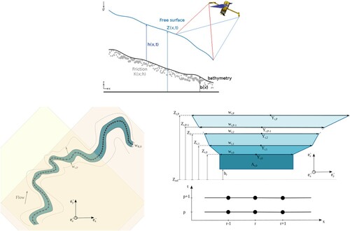
Figure 1. (Up) The inverse problem: infering the flow discharge $Q(x,t)\left({\mathrm{m}}^3{\mathrm{s}}^{-1}\right)$, the bathymetry $b\left(x\right)$ and a friction parameter $K\left(x\right)$ from the WS elevation $Z(x,t)$ at large scale – see below – and every few days only. (Down)(Left) The river measured by SWOT mission: the satellite swaths (large coloured rectangles), the 1D longitudinal grid with the averaged satellite measurements (black dots) along the river centreline (black line). (Down)(Right Top) Effective river cross-section at reach r defined from SWOT measurements $\{Z_{r,p},W_{r,p}{\}}_{R,P+1}$. (Down) (Right Bottom) Resulting space -- time stencil $(r,p)$. x denotes the curvilinear abscissa along the river centreline defined at low flow by $Y_{r,0}$ with $Y_{r,p}$ the middle of the cross-sectional width.

None of the studies aforementioned has fully solved the inverse problem encountered in the satellite context at global scale yet: the inference of the key triplet (discharge $Q(x,t)$, bathymetry $b\left(x\right)$ and friction coefficient $K\left(x\right)$).

Variational Data Assimilation (VDA) approaches (based on the optimal control of the flow model [13–15]) have already been employed to address the present inverse problem. Recall that VDA approaches consists in minimizing a cost function measuring the discrepancy between the model outputs and the observations; thus combining at best the model, the observations and prior information (fields values, characteristic wave length of variations and fields regularity). In some circumstances (depending on the a-priori available information), it is possible to infer the key unknown ‘parameters’ of the river flow model: the inflow discharge $Q_{in}\left(t\right)$, the bathymetry $b\left(x\right)$, the friction K and/or forcing terms (e.g. lateral fluxes). Among the pioneer VDA studies dedicated to hydraulic models, let us cite [16–18]; next [19,20] have inferred the inflow discharge in 2D shallow-water river models. Infering the discharge and complete set of the hydraulic parameters from WS measurements only may lead to ‘equifinality issues’ (ill-posed inverse problems) depending on the adequacy between the observations frequency and the flow dynamics, and the available prior information. The inference of the key triplet (inflow discharge, effective bathymetry and friction coefficient) is investigated in [20,21] but from surface Lagrangian drifting markers providing constraining observations. The upstream, downstream and a few lateral fluxes are identified from water levels measured at in-situ gauging stations (Pearl River, China) in [22]; however again the bathymetry and friction are given. The assimilation of spatially distributed water level observations in a flood plain (a single image acquired by SAR) and a partial in-situ time series (gauging station) are investigated in [23,24], see also [25]. In [26,27] the inference of inflow discharge and lateral fluxes are identified by VDA by superposing a 2D local ‘zoom model’ over the 1D Saint-Venant model; these studies are not conducted in a sparse altimetry measurement context.

The altimetry measurements of WS are generally sparse compared to the flow dynamics, both in space and time. This important feature of the inverse problem is analysed in detail in [28] through the original and instructive ‘identifiability map’. The latter is the $(x,t)$-plane representation of all the available information, that are: the satellite measurements, the model response in terms of wave propagation and the misfit with respect to the equilibrium state.

Concerning the bathymetry inference, it is shown in [7,28,29] that given a single in-situ measurement of bathymetry, the complete bathymetry profile can be reconstructed. [28,30] present accurate inferences of $Q\left(t\right)$ by a similar VDA process as the present one but based on the 1D Saint-Venant flow model ‘only’ (it does not include a hierarchical modelling strategy as in the present approach). In the river case considered in [30], the priors are computed from small Gaussian perturbations of the ‘true’ values of K and b; see also [31] which considers the Po and Garonne rivers. Moreover these priors define a highly controlling rating curve $Q\left(Z\right)$ at downstream (outflow condition) (see [30, Eqs. (6) and (14)]). In other words, the downstream boundary condition of these models is specified as a known, true relationship between river elevation and discharge. As a consequence, the inversion process converges quite easily to the correct discharge $Q\left(t\right)$ and bathymetry $b\left(x\right)$: values corresponding to the nearly exact rating curve.

In summary these recently developed VDA algorithms are accurate to infer the inflow discharge $Q_{in}\left(t\right)$ but from accurate prior information. The latter may be a controlling downstream flow condition [30,32] or a single depth measurement in the river [28].

In view to apply the algorithms to worldwide ungauged rivers, no accurate prior information should be introduced, neither in the direct model nor in the inverse method. This was not the case up to now; on the contrary this is one of the challenging scenarios considered in the present study. To do so, crucial improvements of the aforementioned VDA-based inversions are proposed. Firstly the hierarchical modelling strategy based on dedicated algebraic systems strengthens the robustness of the estimations in particular if a local or large scale value of Q is provided e.g. from a large scale hydrological model.

It is formally demonstrated (and numerically confirmed) that the complete inverse problem may be ill-posed for ungauged rivers (the most challenging case). However a simple good prior mean value of $\overline{Q}$ (or one reference value of bathymetry $b_{ref}$) improves the accuracy of the estimations of the space-time dependent unknowns $\left(Q\right(x,t),b(x);K(x;h\left)\right)$.

The complete inversion strategy presented in this article may provide river discharge estimations at global scale from the upcoming SWOT satellite data (NASA-CNES-CSA space agencies, 2021). Depending on the rivers, additional prior information may be obtained from databases or not. The estimations are valid at observation hours since the observations are propagated by the time-dependent flow model. An identifiability map [28] provides a rough estimation of the estimations range of validity. The numerical experiments scenarios addressed are relatively extensive to cover a large spectrum of realistic contexts and worldwide rivers. Numerical results are analysed for portions of three different rivers ($\sim 100$ km long each); each case presenting a ‘low identifiability index’ (following the definition introduced in [28]). This means that each case presents a high frequency of hydrograph variations compared to the observation frequency. The corresponding inverse problems are relatively challenging, somehow partially ill-posed.

In this study, three different inverse problems are considered. Each of them corresponds to a ‘scenario’:

• Scenario S1): ungauged rivers. The observed river is ungauged: no reliable prior information is available excepted the satellite WS measurements plus a potential Mean Annual Flow (MAF) obtained from a global database.

• Scenario S2): partially gauged river. In this case relatively reliable values of discharge are provided at one location (gauge station) in the portion of the river. These values may be provided by either a global discharge database or a calibrated hydrological model. Furthermore the method for this scenario can be extended to use outputs of hydrological models that provide statistical information (density function, uncertainty, etc.).

• Scenario S3): pointwise measured bathymetry. In this case, one pointwise in-situ measurement of bathymetry $b_{ref}$ (or a cross-section profile) is available.

For each scenario Sn) (n = 1,.., 3), a different computational strategy is developed. Two contexts of observations are considered. ObsFs): a SWOT like fast sampling (Cal-Val) orbit with ∼1 day period; ObsNs): a SWOT like nominal sampling with 21 days period (with 1–4 passes at mid-latitudes).

All the developed algorithms are available in the open-source computational software DassFlow [33].

The outline of the article is as follows. Section 2 presents the river flow models: (a) the classical Saint-Venant equations with altimetry dedicated cross-sections; (b) original altimetry dedicated algebraic flow systems (‘low complexity’ -- ‘low Froude’ systems). These systems are either based on the classical Manning–Strickler's law or on explicit ‘low Froude bathymetry’ expressions. They are useful for different purposes, both direct and inverse computations, and depending on the scenario. Section 3 presents the VDA formulation which takes into account prior hydraulic length scale and error measurement amplitudes. Moreover it is demonstrated (formal calculations) that based on the 1D Saint-Venant equations and WS measurements only, the space-time variations of discharge $Q(x,t)$ may be inferred up to a multiplicative factor only (a ‘bias’ may remain). The descriptions of the three test rivers and the WS measurements are presented in Section 4. The various scenarios (leading to 20 numerical experiments in total) are presented in Section 5. The estimation of the first guesses is an important step of the upcoming inversions by VDA. It depends on the available prior information; their computations are presented in Section 5 too. Section 6 focuses on the ObsFs context: inferences for fast sampling (1 day) and the three scenarios. The numerical results confirm that the space-time variations of the inferred discharge $Q_{in}\left(t\right)$ are (very) accurate, however up to a potential bias. Section 7 focuses on the ObsNs) context and the importance of the identifiability maps' theory to improve the estimations of discharge values. Section 8 presents how to compute Q in real time from newly acquired observations (past the ‘calibration’ – ‘learning’ period). It is done using one of the algebraic - low complexity system presented in Section 2. A conclusion is proposed in Section 9.

2. The river flow models

The primary rivers flow model is the classical Saint-Venant equations in $(A,Q)(x,t)$ variables, see e.g. [4,34], with the Manning–Strickler friction coefficient K defined as a power law in water depth h. It is worth recalling that at the current hydrology satellites measurement scale, the river flows present a low Froude number $F_r$; typically $F_r$ ranges approximatively within $\approx [0.1,0.3]$. A first consequence is that the imposed downstream condition controls the flow; then in lack of prior information, it is important that this outflow condition is as ‘transparent’ as possible (that is no wave is reflected by the outflow condition at the boundary). To do so, a condition related to the normal depth (derived from the equilibrium Manning–Strickler's equation, see e.g. [4,34]) is imposed. A second consequence is the relatively good accuracy of the simple Manning–Strickler's equation to model the flow (see e.g. [6,7,9] for studies in the present SWOT context). However the Manning–Strickler's equation is a scalar algebraic relation highly sensitive to uncertainties; moreover as shown in [7] the actual independent variable of this relation is Q/K and not simply Q. Then below are derived ‘low complexity (algebraic) systems’ which are more robust to the uncertainties of the numerous measurements. These algebraic equations are based on the classical hydraulic assumption ‘low Froude’ hence similar in this sense to the Manning–Strickler's equation, but they natively integrate the numerous WS measurements. The resulting systems are original; they are employed both for direct modelling (real computational time estimations past the calibration period) and inverse modelling (in particular the estimation of first guesses in the VDA inverse method). The inversions of these low complexity systems based on the numerous observations are much robust (less sensitive to the errors, uncertainties) than the usual Manning–Strickler scalar equation.

2.1. The 1D Saint-Venant model

The 1D Saint-Venant equations below are extremely classical in river hydraulics. It is depth-integrated equations relying on the long-wave assumption that is the geometrical ratio of the flow $\epsilon =h^{\ast }/L^{\ast }$ small, $h^{\ast }$ being a characteristic water depth and $L^{\ast }$ a characteristic length scale (shallow-water assumption). In their non-conservative form in $(A,Q)$ variables, A the wetted cross-section $\left[{\mathrm{m}}^2\right]$, Q the discharge $[{\mathrm{m}}^3\cdot {\mathrm{s}}^{-1}]$, the equations read as follows, see e.g. [4]: (1) $\begin{array}{rl}{\mathrm{\partial }}_{t}A+{\mathrm{\partial }}_{x}Q& =0\\ {\mathrm{\partial }}_{t}Q+{\mathrm{\partial }}_x\left(\frac{Q^2}{A}\right)+gA{\mathrm{\partial }}_{x}Z& =-gA{S}_f(A,Q;K)\end{array}$(1)

where g is the gravity magnitude $[\mathrm{m}\cdot {\mathrm{s}}^{-2}]$, Z is the WS elevation $\left[\mathrm{m}\right]$, $Z=(b+h)$ where b is the lowest bed level (bathymetry elevation) $\left[\mathrm{m}\right]$ and h is the water depth $\left[\mathrm{m}\right]$. $S_f$ is the classical Manning–Strickler friction term: (2) $S_f(A,Q;K)=\frac{|Q|Q}{K^2{A}^2{R}_h^{4/3}}$(2) with K the Strickler friction coefficient $[{\mathrm{m}}^{1/3}\cdot {\mathrm{s}}^{-1}]$, $R_h=A/P_h$ the hydraulic radius $\left[\mathrm{m}\right]$, $P_h$ the wetted perimeter. It will be noticed in next section that $R_h$ may be approximated by the water depth h for large rivers. The discharge Q is related to the average cross-sectional velocity u $[\mathrm{m}\cdot {\mathrm{s}}^{-1}]$ : Q = uA. The Strickler friction coefficient K is defined as a power law in h: (3) $K\left(h\right)=\alpha h^{\text{β}}$(3)

where α and β are two constants. This friction coefficient definition is richer than a constant uniform value; it represents a quite general friction law with with two parameters only.

This law may depend on the space variable x too.

At the upstream boundary, the discharge $Q_{in}\left(t\right)$ is imposed. At the downstream boundary, the Manning–Strickler equation depending on the unknowns $(A,Q;K{)}_{out}$ is imposed (it is classically integrated in the Preissmann scheme equations). The initial condition is set as the steady state backwater curve profile: $Z_0\left(x\right)=Z\left(Q_{in}\right(t_0\left)\right)$. This 1D Saint-Venant model is discretized using the classical implicit Preissmann scheme.

2.2. River description from SWOT measurements

The upcoming SWOT measurements will provide time series with spatially distributed measurements of river surface elevation Z and width W, [1]. The measurements will be provided at two different scales:

• The ‘node scale’: $\sim 200$ m long;

• The ‘reach scale’: a few kilometres long.

The altimetry signal at node scale enables measurements of relatively high frequencies variations but with relatively important uncertainties. On the contrary at reach scale the signal measurements is more accurate but capture lower frequencies only. The WS elevations and widths are similarly computed both at reach scale and node scale. The WS slopes are reliable at reach scale only.

Let us decompose the river portion using R ‘points’: r = 1,.., R, see Figure 1. The considered time period is decomposed following $(P+1)$ overpasses: p = 0,.., P. The overpasses are ordered by increasing flow height. The case p = 0 denotes the lowest water level. The SWOT data set on a river portion is: $\{Z_{r,p},W_{r,p}{\}}_{R,P+1}$. At reach scale a third variable is also provided, the slope of the free surface $\{S_{r,p}{\}}_{R,P+1}$. Here these slopes values are computed from the heights values; as a consequence the provided datasets are $\{Z_{r,p},W_{r,p}{\}}_{R,P+1}$.

In what follows the discrete space variable $r,r=1,..,R$, denotes the reach number in the low complexity algebraic systems and the node number (or even the computational grid number if indicated) in the 1D Saint-Venant flow dynamics.

The direct model (1(1) $\begin{array}{rl}{\mathrm{\partial }}_{t}A+{\mathrm{\partial }}_{x}Q& =0\\ {\mathrm{\partial }}_{t}Q+{\mathrm{\partial }}_x\left(\frac{Q^2}{A}\right)+gA{\mathrm{\partial }}_{x}Z& =-gA{S}_f(A,Q;K)\end{array}$(1) ) is considered with the specific cross-sectional geometry shape described in Figure 1. It consists in discrete cross-sections formed by asymmetrical trapezium layers $(Z_{r,p},W_{r,p})$; the centre of each top width (in the cross-flow direction) is denoted by $Y_{r,p}$. In what follows, the WS slope is assumed to be positive: $S_{r,p}=-{\mathrm{\partial }}_r{Z}_{r,p}\ge 0$.

The cross-sectional areas $A_{r,p}$ are defined as follows: $A_{r,p}=A_{r,0}+\delta A_{r,p}=A_{r,0}+{\int }_{Z_{r,0}}^{Z_{r,p}}{W}_r\left(h\right)dh\mathrm{\forall }r\mathrm{\forall }p$. The variations $\delta A_{r,p}$ are approximated by the trapeziums $\delta A_{r,p}\approx \sum _{q=1}^p\frac{1}{2}(W_r^q+W_r^{q-1})(h_r^q-h_r^{q-1})$. The considered width values $W_r^q$ are supposed to be deterministic variables, no uncertainty is considered; the considered values would correspond to the instrument signal mean value. The lowest cross-sectional areas denoted by $A_{r,0}\mathrm{\forall }r$ are unobserved; they are key unknowns of the flow model. They are represented by rectangles, see Figure 1, or any other fixed shape (e.g. a parabola); all the other cross-sectional areas are trapezoidal.

We have: $h_{r,p}\approx R_{r,p}^h\approx \left(A_{r,p}/\right(W_{r,0}+2h_{r,p}+W_{r,p}\left)\right)\mathrm{\forall }r$. This approximation has been numerically verified on all considered rivers. Since W>>h, it follows the effective depth expression: $h_{r,p}=(A_{r,0}+\delta A_{r,p})(W_{r,0}+W_{r,p}{)}^{-1}$.

The unobserved wetted cross-section $A_0$ can be represented by a rectangle, a trapezium, a parabola or even a triangle, by setting: $A_0={\alpha }_A{h}_{0,\alpha }W$ with ${\alpha }_A\in [\frac{1}{2},1]$. However it will be shown that the a-priori effective cross-section shape does not influence the low Froude (‘low complexity’) flow relations, see Section 2.3. We define the hydraulic mean depth $h_0$ by: $h_0=A_0/W$; it is the depth corresponding to an effective rectangular cross-section.

2.3. Low complexity algebraic models

In this section, so-called ‘low complexity systems’ are derived; this terminology ‘low complexity’ being in comparison with the space-time dependent Saint-Venant model which requires higher CPU time computations. Indeed these low complexity systems are algebraic and they are solvable in real-time (Section 8.2). Their equations are based on classical hydraulic assumptions but they are derived in the particular present context: the assimilation of SWOT altimetry data. They natively integrate the measured fields and they may be differently formulated depending on which field is given or unknown. Note that another formulation of the low complexity system is derived in Section A.2 too.

To derive these equations, the basic assumptions made on the flows and data are the following.

(A1) The altimetry measurements are relatively ‘large scale’ compared to the river flows dynamics. In terms of temporal dynamics, since the satellite cannot make infer dynamics much faster than its own frequency revisit (which is $\approx 10$ days), at each observation instant p, the flow may be described as a steady-state flow. In terms of spatial variations, the SWOT instrument will provide an average value of the WS measurement at relatively large scale (RiverObs measurements in the SWOT community [35]). Therefore the flow may be described as locally uniform at the reach length scale.

(A2) At the reach scale defined above, the flow presents low Froude number values; under the low Froude flow assumption, the inertial terms in the momentum equations can be neglected.

(A3) The considered rivers do not present lateral fluxes.

Moreover the considered rivers are wide enough to assume that the hydraulic radius $R_h\approx h$ in the Manning–Strickler friction term $S_f$, see (1(1) $\begin{array}{rl}{\mathrm{\partial }}_{t}A+{\mathrm{\partial }}_{x}Q& =0\\ {\mathrm{\partial }}_{t}Q+{\mathrm{\partial }}_x\left(\frac{Q^2}{A}\right)+gA{\mathrm{\partial }}_{x}Z& =-gA{S}_f(A,Q;K)\end{array}$(1) ).

2.3.1. The low Froude flow model: system of local Manning–Strickler's equations

For example for a rectangular cross-section, the Froude number Fr satisfies: $F{r}^2=u{c}_e^{-1}$ with $c_e$ the wave celerity, $c_e=\sqrt{gh}$. Assuming that the flow is permanent and low Froude, $F{r}^2<<1$, the momentum equation simplifies as the Manning–Strickler law: $Q=KA{h}^{2/3}\sqrt{S}$. Considering this law at each river reach r and each observation time p, this provides the following system: (4) $(K_{r,p}^{-1}{Q}_{r,p}{)}^{3/5}=(A_{0,r}+\delta A_{r,p})W_{r,p}^{-2/5}{S}_{r,p}^{3/10}\mathrm{\forall }r,\mathrm{\forall }p$(4) for each reach $r\in [1\dots R]$ and each satellite pass $p\in [0\dots P]$. The terms $\delta A_{r,p},W_{r,p},S_{r,p}$ are measured, while the terms $Q_{r,p},A_{0,r}$ and $K_{r,p}$ are not.

This system (4(4) $(K_{r,p}^{-1}{Q}_{r,p}{)}^{3/5}=(A_{0,r}+\delta A_{r,p})W_{r,p}^{-2/5}{S}_{r,p}^{3/10}\mathrm{\forall }r,\mathrm{\forall }p$(4) ) can be employed differently depending on the available information and the unknowns. In the inversion computations presented in Section A.2, (4(4) $(K_{r,p}^{-1}{Q}_{r,p}{)}^{3/5}=(A_{0,r}+\delta A_{r,p})W_{r,p}^{-2/5}{S}_{r,p}^{3/10}\mathrm{\forall }r,\mathrm{\forall }p$(4) ) is reformulated in (A2(A2) $D_{c}Bil(\tilde{K},A)+D_d\tilde{K}=\tilde{Q}\text{ in }{R}^{R(P+1)}$(A2) ) to estimate pairs $(K_r^{3/5},A_{r,0})$ from prior discharge values $Q_{r,p}$ (ancillary data).

2.3.2. The effective low Froude bathymetry

By injecting the expression of Q in (4(4) $(K_{r,p}^{-1}{Q}_{r,p}{)}^{3/5}=(A_{0,r}+\delta A_{r,p})W_{r,p}^{-2/5}{S}_{r,p}^{3/10}\mathrm{\forall }r,\mathrm{\forall }p$(4) ) (we suppress the subscripts ${}_{r,p}$) into the mass conservation equation (${\mathrm{\partial }}_{x}Q=0$), it follows: ${\mathrm{\partial }}_x\left(KA{h}^{2/3}{S}^{1/2}\right)=0$. Assuming a constant friction coefficient K, this simplifies to: $\left({\mathrm{\partial }}_{x}h/h\right)\left(x\right)=-\frac{3}{2}\left(\right({\mathrm{\partial }}_x\left(S^{1/2}\right)/S^{1/2})+({\mathrm{\partial }}_{x}A/A\left)\right)\left(x\right)$.

Next, following [29] and given a reference depth value $h_{ref}$ (measured at one reference reach ref), the explicit expression of h follows: $h\left(x\right)=h_{ref}(A{S}^{1/2}{)}_{ref}^{3/2}\cdot (A{S}^{1/2}{)}^{-3/2}\left(x\right)$. This estimation of water depth h is analysed in detail in [7,29].

Let us extend this estimation of the water depth h (hence the bed elevation b) to the present context, that is from a complete set of WS measurements. If considering an effective cross-sectional area $A={\alpha }_{A}hW$ with ${\alpha }_A\in [\frac{1}{2},1]$ then the bathymetry expression reads: $b\left(x\right)=Z\left(x\right)-C_{ref}\cdot {\alpha }_A^{-3/5}\left(x\right)\cdot \left(W{S}^{1/2}{)}^{-3/5}\right(x)$ with $C_{ref}=h_{ref}\left({\alpha }_{A}W{S}^{1/2}\right){|}_{ref}^{3/5}$. The three parameters $({\alpha }_A,W,S)$ describe the three dimensions of the flow.

Given the WS measurements $(Z,W,S)$ and the value $S_{ref}$ at an arbitrary reach ref, this explicit expression of $b\left(x\right)$ provides an effective bathymetry. Observe that the effective bathymetry elevation b is equivalent if considering different wetted cross-section shapes determined by ${\alpha }_A$. In other words, in the present low Froude relations, the shape of the effective cross-sectional area A may be chosen arbitrarily. In the following we set ${\alpha }_A=1$; that is a rectangular effective shape. Finally the effective bathymetry expression under Assumptions (A1)–(A3) previously mentioned reads: (5) $b_r+(Z_{ref,p}-b_{ref})\cdot {\mathcal{O}}_{ref,p}^{-1}\cdot {\mathcal{O}}_{r,p}=Z_{r,p}\mathrm{\forall }r,r\ne ref,\mathrm{\forall }p\ge 0$(5) with the observational term ${\mathcal{O}}_{r,p}=(W_{r,p}\sqrt{S_{r,p}}{)}^{-3/5}\mathrm{\forall }r\mathrm{\forall }p$. (The only observational terms of this estimation are Z and the product $W{S}^{1/2}\equiv \mathcal{O}$ .)

In the following the bathymetry $\{b_r{\}}_r$ solution of (5(5) $b_r+(Z_{ref,p}-b_{ref})\cdot {\mathcal{O}}_{ref,p}^{-1}\cdot {\mathcal{O}}_{r,p}=Z_{r,p}\mathrm{\forall }r,r\ne ref,\mathrm{\forall }p\ge 0$(5) ) is called the ‘Low Froude bathymetry’.

The system (5(5) $b_r+(Z_{ref,p}-b_{ref})\cdot {\mathcal{O}}_{ref,p}^{-1}\cdot {\mathcal{O}}_{r,p}=Z_{r,p}\mathrm{\forall }r,r\ne ref,\mathrm{\forall }p\ge 0$(5) ) contains $(P+1)\times (R-1)$ equations (given 1 reference reach only) with R unknowns: the bathymetry vector $b=\left(\right\{b_r{\}}_r,b_{ref})r\in [1,R],r\ne ref$. The system reads: $(A.b{)}_p=(F{)}_p\mathrm{\forall }p$, with$(F_r{)}_p=Z_{r,p}-Z_{ref,p}{\mathcal{O}}_{ref,p}^{-1}\cdot {\mathcal{O}}_{r,p}$ and the $(R-1)(P+1)\times R$ matrix $(A{)}_p=[I_{(R-1\times R-1)}|{\mathcal{O}}_{ref,p}^{-1}\cdot {\mathcal{O}}_{r,p}]$. For $P\ge 1$, A is of maximal rank excepted if the observational vectors $({\mathcal{O}}_r{)}_p$ are linearly dependent; that is not the case if the considered water flow lines represent flow variations.

On the coupled influence between b and a non constant friction coefficient K. As shown above and already demonstrated in [7,29], the low Froude assumption enables to separate the bathymetry effect from the friction effect if the friction coefficient K is constant, see (5(5) $b_r+(Z_{ref,p}-b_{ref})\cdot {\mathcal{O}}_{ref,p}^{-1}\cdot {\mathcal{O}}_{r,p}=Z_{r,p}\mathrm{\forall }r,r\ne ref,\mathrm{\forall }p\ge 0$(5) ); K does not appear anymore in (5(5) $b_r+(Z_{ref,p}-b_{ref})\cdot {\mathcal{O}}_{ref,p}^{-1}\cdot {\mathcal{O}}_{r,p}=Z_{r,p}\mathrm{\forall }r,r\ne ref,\mathrm{\forall }p\ge 0$(5) ). On the contrary, if K varies in space or depends on the depth h, like in (3(3) $K\left(h\right)=\alpha h^{\text{β}}$(3) ) or in the Einstein formula, see e.g. [4], then K and b have a coupled influence even at low Froude. Typically if considering the following power law: $K\left(h\right)=K_0\cdot (h-h_0{)}^{\text{β}}(x)$ with gradually varied coefficients i.e. ${\mathrm{\partial }}_x{K}_0\sim 0\sim {\mathrm{\partial }}_x\text{β}$, after calculations the depth expression reads: $\left[h\right(x)\cdot |h(x)-h_0{|}^{3\text{β}/2}]=c_0\cdot \left(A{S}^{1/2}{)}^{-3/2}\right(x)$ with $c_0=|h_{ref}-h_0{|}^{3\text{β}/2}\cdot h_{ref}\cdot (A{S}^{1/2}{)}_{ref}^{+3/2}$ ($h_{ref}$ the reference depth value). The case K constant is recovered from the equation above by setting $\text{β}=0$.

Relationship with empirical laws. It may be practical to consider empirical laws based on hydraulic geometry such as: $Z_{r,p}=b_r+a_r{W}_{r,p}^{\text{β}}$. In other respects, (5(5) $b_r+(Z_{ref,p}-b_{ref})\cdot {\mathcal{O}}_{ref,p}^{-1}\cdot {\mathcal{O}}_{r,p}=Z_{r,p}\mathrm{\forall }r,r\ne ref,\mathrm{\forall }p\ge 0$(5) ) can be re-written as follows: $Z_{r,p}=b_r+C_{ref,p}\cdot {\alpha }_{A,r}^{-3/5}\cdot \left(W{S}^{1/2}\right){|}_{r,p}^{-3/5}\mathrm{\forall }r,\mathrm{\forall }p,p=0,..,P$ with $C_{ref,p}=h_{ref,p}({\alpha }_{A}W{S}^{1/2}{)}_{ref,p}^{3/5}$. We assume constant cross-section shapes (${\alpha }_{A,r}={\alpha }_A\mathrm{\forall }r$). By equalling the two estimations it follows: $W_{r,p}^{\text{β}}\cdot (W_{r,p}{S}_{r,p}^{1/2}{)}^{3/5}=a_r^{-1}\cdot h_{ref,p}(W{S}^{1/2}{)}_{ref,p}^{3/5}\mathrm{\forall }r\mathrm{\forall }p$. Assuming that the flow is uniform in terms of the observational term $\left(W{S}^{1/2}\right)$ i.e. this quantity is constant for the considered reaches, we obtain that: $W_p^{\text{β}}=a^{-1}{h}_p$; equivalently: $Z_p=b+a{W}_p^{\text{β}}$.Therefore the low Froude estimation (5(5) $b_r+(Z_{ref,p}-b_{ref})\cdot {\mathcal{O}}_{ref,p}^{-1}\cdot {\mathcal{O}}_{r,p}=Z_{r,p}\mathrm{\forall }r,r\ne ref,\mathrm{\forall }p\ge 0$(5) ) contains empirical laws of the form indicated above. Given β and time series of WS elevation and width this relation allows to infer an effective river bed elevation e.g. as in [5]. Such law could be defined in function of hydraulic geometry knowledge.

On the accuracy of these low Froude - low complexity systems. The two systems (4(4) $(K_{r,p}^{-1}{Q}_{r,p}{)}^{3/5}=(A_{0,r}+\delta A_{r,p})W_{r,p}^{-2/5}{S}_{r,p}^{3/10}\mathrm{\forall }r,\mathrm{\forall }p$(4) ) and (5(5) $b_r+(Z_{ref,p}-b_{ref})\cdot {\mathcal{O}}_{ref,p}^{-1}\cdot {\mathcal{O}}_{r,p}=Z_{r,p}\mathrm{\forall }r,r\ne ref,\mathrm{\forall }p\ge 0$(5) ) turn out to be reasonably accurate in the present altimetry context (Assumptions (A1)–(A3)). Employed as direct modelling, their solutions have been numerically assessed in [7]; it is done in the present context too, see Section 6.2.

3. The variational data assimilation (VDA) formulation

The VDA method employed in the study is presented. Moreover a simple formal re-scaling calculation of the Saint-Venant equations is derived; it shows the ill-posedness of the inverse problem if no additional in-situ data is provided.

3.1. The control parameter

Given the WS measurements at nodes scale (see Section 2.2), the VDA method aims at estimating the ‘input parameters’ of the Saint-Venant flow model that is: the inflow discharge $Q_{in}\left(t\right)$ of the Saint-Venant model, the bathymetry $b\left(x\right)$ and the friction coefficient $K\left(h\right)$ defined by (3(3) $K\left(h\right)=\alpha h^{\text{β}}$(3) ). In discrete form, this unknown ‘parameter’ reads: (6) $c={\left(Q_{in,0},\dots ,Q_{in,P};b_1,\dots ,b_N;\alpha ,\text{β}\right)}^T$(6) In (6(6) $c={\left(Q_{in,0},\dots ,Q_{in,P};b_1,\dots ,b_N;\alpha ,\text{β}\right)}^T$(6) ) the subscript p denotes the instant, $p\in \left[\mathrm{0..}P\right]$, α and β are the friction law parameters defined by (3(3) $K\left(h\right)=\alpha h^{\text{β}}$(3) ) and N denotes the computational grid number. The latter contains $\approx 4$ computational grid points per node r, r = 1,.., R. Recall that the VDA method combined to the Saint-Venant flow model is applied at the node scale and not at the ‘reach scale’. Indeed this enables to capture the ‘high frequencies’ contained in the observations.

Given the bijection function between the elevation Z and the cross-sectional area A described in Section 2.2, measuring Z is equivalent to measure A. Of course the parameters used for imposing a normal depth at downstream, see Section 2.1, are considered as unknown; otherwise it would be equivalent to impose an exact outflow condition which highly control the model solution.

3.2. The optimization problem

To estimate the unknown parameter vector c, the VDA consists to minimize a cost function j. The latter is defined by: (7) $j\left(c\right)=j_{obs}\left(c\right)+\gamma j_{reg}\left(c\right)$(7) The term $j_{obs}\left(c\right)$ measures the misfit between the observations and the model output: (8) $j_{obs}\left(c\right)=\frac{1}{2}{∥\left(Z\left(\mathrm{c}\right)-Z_{obs}\right)∥}_N^2$(8) The norm N is defined from the a-priori covariance operator N (a positive definite matrix): $\parallel \cdot {\parallel }_N=\parallel N^{1/2}\cdot {\parallel }_2$. The regularization term $j_{reg}\left(c\right)$ is detailed below; the weighting coefficient $\gamma >0$ is set following an iterative regularization strategy detailed below.

The WS elevation Z depends on c through the flow model (1(1) $\begin{array}{rl}{\mathrm{\partial }}_{t}A+{\mathrm{\partial }}_{x}Q& =0\\ {\mathrm{\partial }}_{t}Q+{\mathrm{\partial }}_x\left(\frac{Q^2}{A}\right)+gA{\mathrm{\partial }}_{x}Z& =-gA{S}_f(A,Q;K)\end{array}$(1) ). The inverse problem reads as: ${\displaystyle c^{\ast }=\mathrm{a}\mathrm{r}\mathrm{g}\mathrm{m}\mathrm{i}\mathrm{n}\mathrm{j}\left(c\right)}$.This minimization problem of (1(1) $\begin{array}{rl}{\mathrm{\partial }}_{t}A+{\mathrm{\partial }}_{x}Q& =0\\ {\mathrm{\partial }}_{t}Q+{\mathrm{\partial }}_x\left(\frac{Q^2}{A}\right)+gA{\mathrm{\partial }}_{x}Z& =-gA{S}_f(A,Q;K)\end{array}$(1) ) is numerically solved by a Quasi-Newton descent algorithm (here the classical L-BFGS algorithm presented in [36]). This first order method requires the computation of the cost gradient $\mathrm{\nabla }j\left(c\right)$. The gradient is computed by introducing the adjoint model (enabling to consider large control vector dimensions). The adjoint code is obtained by employing the automatic differentiation tool Tapenade [37]. We refer to the pioneer studies [14,15,38,39] for VDA concepts; see also e.g. the online detailed courses [38,39] for details on thee approach.

The unknown parameter c contains three variables of different physical nature which are space and/or time dependent. Moreover the bathymetry $b\left(x\right)$ and the friction coefficient $K\left(h\right)$ are correlated and they may have a similar influence in terms of WS signature therefore leading to an ill-posed inverse problem, see e.g. [7] for such a discussion in the present inversion context. Then the inverse problem is regularized in two ways following relatively classical techniques.

Firstly, the regularization term $j_{reg}$, see (7(7) $j\left(c\right)=j_{obs}\left(c\right)+\gamma j_{reg}\left(c\right)$(7) ) is simply set as: $j_{reg}\left(c\right)=\frac{1}{2}\parallel b\mathrm{\prime }\mathrm{\prime }\left(x\right){\parallel }_2^2$. $j_{reg}$ imposes a smoothing effect on the inferred bathymetry profiles $b\left(x\right)$). Secondly the following metrics based on (classical) covariance operators are introduced.

3.3. Covariance operators and change of control variable

The following natural change of variable is made, [40,41]: (9) $k=B^{-1/2}(\mathrm{c}-{\mathrm{c}}_{prior})$(9) where B is a covariance matrix. Recall that the unknown parameter (the control variable) c is defined by (6(6) $c={\left(Q_{in,0},\dots ,Q_{in,P};b_1,\dots ,b_N;\alpha ,\text{β}\right)}^T$(6) ); $c_{prior}$ is a prior value (also called ‘background’ or ‘first-guess’ value). The value of $c_{prior}$ depends on the prior information.

The choice of B may be viewed as an important prior information too since the optimal solution $k^{\ast }$ (strongly) depends on B. Indeed, after this change of variable, the optimality condition reads: $B^{1/2}\mathrm{\nabla }j\left(c\right)=0$. This change of variable may be viewed as a preconditioning method, see e.g. [42,43] for detailed analysis in a different context. Then the optimization problem to be solved re-reads as: (10) $\underset{k}{min}\mathrm{J}\left(k\right)$(10) with $\mathrm{J}\left(k\right)=j\left(c\right)$, j defined by (7(7) $j\left(c\right)=j_{obs}\left(c\right)+\gamma j_{reg}\left(c\right)$(7) ) and the control vector k defined by (9(9) $k=B^{-1/2}(\mathrm{c}-{\mathrm{c}}_{prior})$(9) ). The unknown parameter k contains the three variables $Q_{in}\left(t\right)$, $b\left(x\right)$, $K\left(h\right)$ in their discrete form. These three variables are assumed to be uncorrelated: B is thus defined as a block diagonal matrix. We set: (11) $B=\left(\begin{array}{ccc}{B}_Q& 0& 0\\ 0& B_b& 0\\ 0& 0& B_K\end{array}\right)$(11) Each block $B_{◻}$ is defined as a covariance matrix (positive definite matrix). The matrices $B_Q$ and $B_b$ are set as classical second order auto-regressive correlation matrices, see e.g. [41,43,44]: (12) ${\left(B_Q\right)}_{i,j}=({\sigma }_Q{)}^2\exp \left(-\frac{\left|t_j-t_i\right|}{\mathrm{\Delta }{t}_Q}\right)\text{ and }{\left(B_b\right)}_{i,j}=({\sigma }_b{)}^2\exp \left(-\frac{\left|x_j-x_i\right|}{L_b}\right)$(12) The parameters $\mathrm{\Delta }{t}_Q$ and $L_b$ act as correlation lengths. Given the observation frequency (1 day minimum), given the measurements spacing (200m long ‘observation pixels’) and given the typical Froude number of the observed river flows, adequate values for these parameters are: $\mathrm{\Delta }{t}_Q=24$ h and $L_b=1$ km. We refer to [28] for a thorough analysis of the discharge inference in terms of frequencies and wave lengths. The matrix $B_K$ is diagonal; it may be (roughly) set as: $B_K=diag({\sigma }_{\alpha }^2,{\sigma }_{\text{β}}^2)$. The scalar values ${\sigma }_{◻}$ may be viewed as variances.

This VDA formulation above takes into account prior hydraulic scales through the parameters $\mathrm{\Delta }{t}_Q$ and $L_b$; the balance between the different control variables are set through the parameters ${\sigma }_{◻}$. Their values are detailed in the numerical results sections (Sections 6 and 7).

On the non over-fitting of data. Let us denote by δ the noise level such that for all locations $\parallel Z_{obs}-Z_{true}{\parallel }^2\le \delta$ with $Z_{obs}$ the observed and $Z_{true}$ the true WS elevation.

Following the Morozov discrepancy principle, see e.g. [45] and references therein, the regularization parameter γ in (7(7) $j\left(c\right)=j_{obs}\left(c\right)+\gamma j_{reg}\left(c\right)$(7) ) is chosen a-posteriori such that j does not decrease below the noise level. In the present numerical experiments, the convergence is stopped if $j_{obs}\left(c\right)\le \chi \delta$ with $\chi \sim 0.9$.

On the potentially ill-posed inverse problem. In Appendix, we show that the inverse problem based on the 1D Saint-Venant equations and the WS data only (no additional in-situ data is available even not a mean value) is ill-posed in the sense its solution is defined to a multiplicative factor. Consult Section A.1 for details.

4. Test rivers description

In this section the three test rivers with the associated data (WS measurements) are presented. The three test rivers consist of 75 km of the Garonne River (France), 98 km of the Po River (Italy) and 147 km of the Sacramento River (California, USA), see Table 1. These three rivers have contrasting morphological characteristics in terms of the slope variability and cross-section shapes.

Table 1. Hydraulic characteristics for each test river.

River	Reach length (km)	Max. width (m)	Avg. slope (m km${}^{-1}$)	Avg. flow (m${}^3{\mathrm{s}}^{-1}$)	Froude range (–)
Garonne	75	49/1383	0.861	156	0.03–0.67
Po	98	116/5515	0.145	1499	0.04–0.47
Sacramento	147	59/678	0.558	251	0.02–0.64

The numerical inversions of the WS measurements are performed in two different observational contexts. (a) The SWOT Cal/Val (Calibration/Validation) period measurements of the satellite corresponding to a temporary low orbit providing daily observations; this is the ObsFs context. This context is considered for the Po and the Garonne rivers. (b) The nominal SWOT spatio-temporal sampling providing unfrequent observations (1–4 observations per $\approx 21days$ repeat cycle); this is the ObsNs context. This context is considered for the Sacramento river only.

The WS measurements consist in sets of $(Z_{r,p},W_{r,p}{)}_{R,P+1}$: (a) either numerically computed with daily frequency (ObsFs) context); (b) or using the SWOT Hydrology Simulator with few days frequency (ObsNs context).

SWOT Hydrology Simulator outputs (ObsNs context) are available for Sacramento river only so the considered data for the two other rivers (Garonne and Po) are synthetic: they are obtained by adding Gaussian errors to outputs of a reference hydraulic model. In this case we have: $Z_{obs}(x,t)=Z_{true}(x,t)+\mathcal{N}(0,{\sigma }_Z)$ with ${\sigma }_Z=25$cm. This value of ${\sigma }_Z$ corresponds to the expected magnitude of SWOT measurement errors, see [1]. The observation period is $\mathrm{\Delta }{t}_{obs}=1$ day; this corresponds to the Cal/Val (Calibration/Validation) phase of the satellite mission (ObsFs context).

For the Sacramento case, the observations are simulated by the SWOT Hydrology Simulator, corresponding to a nominal 21 days SWOT cycle. The whole river portion is observed by SWOT (from two tracks) at the 9th and 19th days of each 21 days repeat cycle. The measurement error on Z is characterized by an average variance ${\sigma }_Z=34$ cm, see Table 1. It is interesting to consider this large amplitude error in case of the real SWOT errors is higher than the scientific requirements, [1]. For the three cases the spatial sampling is $\mathrm{\Delta }{x}_{obs}=200$ m; the SWOT Hydrology Simulator outputs are averaged in space on $\sim 200$ m nodes (corresponding to the so-called RiverObs nodes).

5. The different scenarios and corresponding first guesses

In this section the three different scenarios S1)–S3) are detailed. The method to compute the first guesses (first values in the iterative VDA method) may depend on the scenario; it is presented in a next section. Finally a summary of the resulting 16 numerical experiments is presented.

5.1. The three different scenarios S1)–S3)

The capabilities of the present inverse method(s) are tested in three scenarios of increasing difficulty. All scenarios are based on a set of SWOT observations $(Z_{r,p},W_{r,p}{)}_{R,P+1}$ ($R\times (P+1)$ WS measurements). The three scenarios are as follows.

1. Scenario S1): ungauged rivers. The observed river is ungauged: no reliable prior information is available (excepted the WS measurements). Only a rough estimation of the mean flow can be used. In the SWOT Science Team, a Mean Annual Flow (MAF) is considered as a valid prior for ‘ungauged’ rivers. This corresponds to the most challenging inverse problem. It is addressed in Sections 6.1 and 7.2.

2. Scenario S2): partially gauged river. In this case ‘relatively reliable’ values of discharge, at least $(R+1)$ values, see (4(4) $(K_{r,p}^{-1}{Q}_{r,p}{)}^{3/5}=(A_{0,r}+\delta A_{r,p})W_{r,p}^{-2/5}{S}_{r,p}^{3/10}\mathrm{\forall }r,\mathrm{\forall }p$(4) ), are provided at one location in the river portion. These values may be provided by either a global discharge database or a calibrated hydrological model. The method presented here can also be extended to take into account statistical information (density functions) or uncertainty if the discharge values are computed using hydrological modelling. This scenario is addressed in Section 6.2.

3. Scenario S3): one bathymetry measurement $b_{ref}$ is available in the river portion. This enables to first estimate the so-called effective low-Froude bathymetry, next to infer the pair $(Q_{in,p},K_{r,p}{)}_{R,P}$. This scenario is addressed in Sections  6.3 and 7.3.

5.2. First guesses computation

The complete control vector c, see (6(6) $c={\left(Q_{in,0},\dots ,Q_{in,P};b_1,\dots ,b_N;\alpha ,\text{β}\right)}^T$(6) ) and (9(9) $k=B^{-1/2}(\mathrm{c}-{\mathrm{c}}_{prior})$(9) ), contains $(P+N+2)$ components: $c=(Q_{in,0}^{\left(0\right)},\dots ,Q_{in,P}^{\left(0\right)};b_1^{\left(0\right)},\dots ,b_N^{\left(0\right)};{\alpha }^{\left(0\right)},{\text{β}}^{\left(0\right)}{)}^T$. A first value has to be set; it is the first guess denoted by $c^{\left(0\right)}$.

For all scenarios S1)–S3), the first-guess value $Q_{in}^{\left(0\right)}$ is computed as follows.

First-guess value $Q_{in}^{\left(0\right)}$. At inflow, we set: $Q_{in}^{\left(0\right)}\left(t_p\right)=Q_{MAF}\mathrm{\forall }p\in [0\dots P]$, where $Q_{MAF}$ is a Mean Annual Flow (MAF) value obtained either from the SWOT a-priori river database under construction [48,49] or from the global Water Balance Model (WBM) [50].

First-guess value $K^{\left(0\right)}$. In scenarios S1) and S3), a constant value of the friction coefficient $K^{\left(0\right)}$ is derived from the SWOT a-priori river database. The considered constant $K^{\left(0\right)}$ values are 25 (resp. 33 and 25) $[{\mathrm{m}}^{1/3}\cdot {\mathrm{s}}^{-1}]$ for the Garonne river (resp. Po and Sacramento rivers). Since constant, these values correspond to the values of ${\alpha }^{\left(0\right)}$ and ${\text{β}}^{\left(0\right)}=0$, see (3(3) $K\left(h\right)=\alpha h^{\text{β}}$(3) ).

In Scenario S2), multiple prior values of discharge are provided. Then the algebraic system (4(4) $(K_{r,p}^{-1}{Q}_{r,p}{)}^{3/5}=(A_{0,r}+\delta A_{r,p})W_{r,p}^{-2/5}{S}_{r,p}^{3/10}\mathrm{\forall }r,\mathrm{\forall }p$(4) ) (see also (A1(A1) $c_{r,p}\cdot K_{r,p}^{3/5}{A}_{r,0}+d_{r,p}\cdot K_{r,p}^{3/5}=Q_{r,p}^{frac35}\text{for all }(r,p)$(A1) )) is solved to obtain $K^{\left(0\right)}$ (actually ${\alpha }^{\left(0\right)}$) and the corresponding effective bathymetry $(b_r{)}_{r=1,\dots ,R}$.

Observe that given the lowest flow WS measurements, defining $(b_r{)}_{r=1,\dots ,R}$ is equivalent to define the unmeasured lowest cross sectional areas $(A_{r,0}{)}_{r=1,\dots ,R}$ since a shape assumption is assumed (e.g. rectangular).

First-guess value $b^{\left(0\right)}$. The computation of $b^{\left(0\right)}$ depends on the scenario.

• Scenario S1) bathymetry (ungauged river). $b^{\left(0\right)}$ is computed by inverting the Manning–Strickler Equation (4(4) $(K_{r,p}^{-1}{Q}_{r,p}{)}^{3/5}=(A_{0,r}+\delta A_{r,p})W_{r,p}^{-2/5}{S}_{r,p}^{3/10}\mathrm{\forall }r,\mathrm{\forall }p$(4) ) with $K^{\left(0\right)}$ and $Q_{in}^{\left(0\right)}$ setup as previously described. (4(4) $(K_{r,p}^{-1}{Q}_{r,p}{)}^{3/5}=(A_{0,r}+\delta A_{r,p})W_{r,p}^{-2/5}{S}_{r,p}^{3/10}\mathrm{\forall }r,\mathrm{\forall }p$(4) ) is a scalar equation; its WS parameters are those of the median observed flow line.

• Scenario S2) bathymetry (partially gauged river). $b^{\left(0\right)}$ is obtained by inverting the algebraic system (A1(A1) $c_{r,p}\cdot K_{r,p}^{3/5}{A}_{r,0}+d_{r,p}\cdot K_{r,p}^{3/5}=Q_{r,p}^{frac35}\text{for all }(r,p)$(A1) ). To be invertible, (A1(A1) $c_{r,p}\cdot K_{r,p}^{3/5}{A}_{r,0}+d_{r,p}\cdot K_{r,p}^{3/5}=Q_{r,p}^{frac35}\text{for all }(r,p)$(A1) ) has to be based on sufficiently numerous different flow lines.

  Note that the estimation of $b^{\left(0\right)}$ computed from the scalar Manning–Strickler Equation (4(4) $(K_{r,p}^{-1}{Q}_{r,p}{)}^{3/5}=(A_{0,r}+\delta A_{r,p})W_{r,p}^{-2/5}{S}_{r,p}^{3/10}\mathrm{\forall }r,\mathrm{\forall }p$(4) ) is much more sensitive to errors (e.g. those of the prior values $(Q^{\left(0\right)},K^{\left(0\right)})$) than if computed from the algebraic system  (A1(A1) $c_{r,p}\cdot K_{r,p}^{3/5}{A}_{r,0}+d_{r,p}\cdot K_{r,p}^{3/5}=Q_{r,p}^{frac35}\text{for all }(r,p)$(A1) ).

• Scenario S3) bathymetry. One in-situ bathymetry measurement (denoted by $b_{ref}$) is available. Then an effective bathymetry profile $(b_r^{\left(0\right)}{)}_{r=1,\dots ,R}$ is derived from (5(5) $b_r+(Z_{ref,p}-b_{ref})\cdot {\mathcal{O}}_{ref,p}^{-1}\cdot {\mathcal{O}}_{r,p}=Z_{r,p}\mathrm{\forall }r,r\ne ref,\mathrm{\forall }p\ge 0$(5) ) and the WS measurements. It is the so-called Low-Froude bathymetry.

The first-guess value $b^{\left(0\right)}$ is estimated at the reach scale (see Section 2.2 for the reach scale definition). Next, the values at the computational grid points $(b_1^{\left(0\right)},..,b_N^{\left(0\right)})$ are derived by linear interpolation.

For Sacramento river, not sufficiently numerous WS observations were available to invert the algebraic system (A1(A1) $c_{r,p}\cdot K_{r,p}^{3/5}{A}_{r,0}+d_{r,p}\cdot K_{r,p}^{3/5}=Q_{r,p}^{frac35}\text{for all }(r,p)$(A1) ) (17 overpasses only were available). As a consequence, Scenario S2) cannot be considered for the Sacramento river.

A comparison of the estimations of $b^{\left(0\right)}$ obtained following these three methods is presented in the next section.

For all cases (see Table 2) we have: $\begin{array}{rl}& \mathrm{\Delta }{x}_{obs}\equiv [r,(r+1\left)\right]\approx 200\mathrm{m},{\sigma }_Z=25\mathrm{c}\mathrm{m},{\sigma }_{{\alpha }_K}=0.5{\mathrm{m}}^{1/3}\cdot {\mathrm{s}}^{-1},\\ & {\sigma }_{{\text{β}}_K}=0.01\text{ and }{\sigma }_b=25\mathrm{c}\mathrm{m}\end{array}$ The criteria used to evaluate the performance of the estimations are the following classical RMSE and relative RMSE at assimilation times: $RMSE=\sqrt{\frac{\sum _{t=1}^n(Q_t^{est}-Q_t^{true}{)}^2}{n}},rRMSE=\sqrt{\frac{1}{n}\sum _{t=1}^n{\left(\frac{Q_t^{est}-Q_t^{true}}{Q_t^{true}}\right)}^2}$ with $Q_{in}^{est}$ (resp. $Q_{in}^{true}$) the estimated (resp. observed) value of inflow discharge at assimilation time t.

Table 2. Summary of the numerical experiments (*: two overpasses at days 9 and 19 every 21 days repeat period).

Case name	Scenario	River	${\sigma }_Z^{perturb}$	$\mathrm{\Delta }{t}_{obs}$	${\sigma }_Q$
S1.Ga.0	S1)	Garonne	0	1 day	15 m${}^3{\mathrm{s}}^{-1}$
S1.Po.0	S1)	Po	0	1 day	71 m${}^3{\mathrm{s}}^{-1}$
S1.Ga.σ	S1)	Garonne	25 cm	1 day	15 m${}^3{\mathrm{s}}^{-1}$
S1.Po.σ	S1)	Po	25 cm	1 day	71 m${}^3{\mathrm{s}}^{-1}$
S2.Ga.0	S2)	Garonne	0	1 day	15 m${}^3{\mathrm{s}}^{-1}$
S2.Po.0	S2)	Po	0	1 day	71 m${}^3{\mathrm{s}}^{-1}$
S2.Ga.σ	S2)	Garonne	25 cm	1 day	15 m${}^3{\mathrm{s}}^{-1}$
S2.Po.σ	S2)	Po	25 cm	1 day	71 m${}^3{\mathrm{s}}^{-1}$
S3.Ga.0	S3)	Garonne	0	1 day	15 m${}^3{\mathrm{s}}^{-1}$
S3.Po.0	S3)	Po	0	1 day	71 m${}^3{\mathrm{s}}^{-1}$
S3.Ga.σ	S3)	Garonne	25 cm	1 day	15 m${}^3{\mathrm{s}}^{-1}$
S3.Po.σ	S3)	Po	25 cm	1 day	71 m${}^3{\mathrm{s}}^{-1}$
S1.Sa.0	S1)	Sacramento	0	21 days*	20 m${}^3{\mathrm{s}}^{-1}$
S1.Sa.σ	S1)	Sacramento	34 cm	21 days*	20 m${}^3{\mathrm{s}}^{-1}$
S3.Sa.0	S3)	Sacramento	0	21 days*	20 m${}^3{\mathrm{s}}^{-1}$
S3.Sa.σ	S3)	Sacramento	34 cm	21 days*	20 m${}^3{\mathrm{s}}^{-1}$

5.3. Inference of an effective bathymetry $b^{\left(0\right)}$ (equivalently $A_0$)

In the ‘complete’ inverse problem solved by VDA, the control vector $\mathrm{c}$, see (6(6) $c={\left(Q_{in,0},\dots ,Q_{in,P};b_1,\dots ,b_N;\alpha ,\text{β}\right)}^T$(6) ), is composed by the upstream discharge, the friction parameter and the bathymetry. However infering by VDA the pair $\left(Q\right(t);K(h\left)\right)$ given the bathymetry b is much less challenging than infering the complete triplet $\left(Q\right(t);K(h);b(x\left)\right)$, see e.g. [28]. As a consequence infering first a (reliable) prior bathymetry profile before performing the iterative VDA process may be interesting. In this section, different alternatives to estimate an effective bathymetry $(b_n{)}_{\mathrm{1..}N}$ are compared. The latter is either employed as the first-guess value $b^{\left(0\right)}$ in the VDA process or may be considered as the (final) estimation.

Given one flow line measurement, the (scalar) Manning–Strickler equation provides the corresponding bathymetry profile $b^{\left(0\right)}$. Obviously this basic approach is highly sensitive to the errors made on the prior values prior values $(Q^{\left(0\right)};K^{\left(0\right)})$. If solving the algebraic system (A1(A1) $c_{r,p}\cdot K_{r,p}^{3/5}{A}_{r,0}+d_{r,p}\cdot K_{r,p}^{3/5}=Q_{r,p}^{frac35}\text{for all }(r,p)$(A1) ) based on multiple flow lines measurements, the resulting estimation of $b^{\left(0\right)}$ is naturally less sensitive to the errors made on the prior values $(Q^{\left(0\right)};K^{\left(0\right)})$.

A third method consists to solve the ‘low Froude bathymetry’ equation (5(5) $b_r+(Z_{ref,p}-b_{ref})\cdot {\mathcal{O}}_{ref,p}^{-1}\cdot {\mathcal{O}}_{r,p}=Z_{r,p}\mathrm{\forall }r,r\ne ref,\mathrm{\forall }p\ge 0$(5) ). Since based on one in-situ measurement $b_{ref}$, the resulting estimation is more robust and accurate than those obtained in Scenario S1).

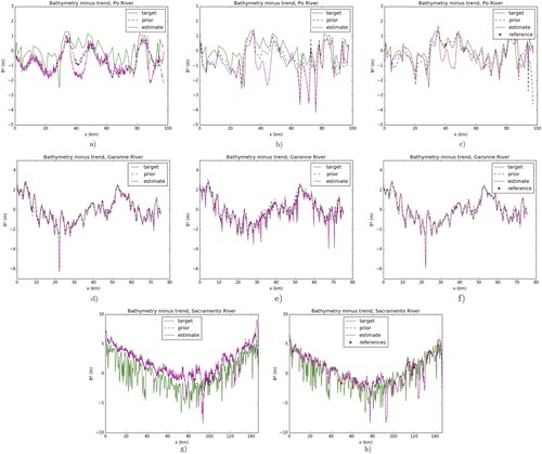
The first two approaches are compared for the Po and Garonne Rivers only on Figure 2 ($B^{\ast }$ represents the bed elevation b minus an average bathymetry trend). The first and third approach are compared for the three Rivers on Figure 2.

Figure 2. True and inferred bathymetry deviation from trend $(B^{\ast }{)}_{\mathrm{1..}N}$ compared to prior bathymetry estimations, noisy observations (Section 5.2): (a,d,g) Scenario S1) bathymetry. (b,e) Scenario S2) bathymetry. (c,f,h) Scenario S3) bathymetry.

In the Sacramento river case, a drift of the estimation (increasing error in space) rises with distance to the reference point $b_{ref}$. Indeed if the basic steady-state condition ${\mathrm{\partial }}_{x}Q=0$ in the ‘Low Froude' equation is not fully satisfied. Moreover a drift in space naturally appears since the model is a first order differential equation. Typical drift amplitudes are presented in [7]. In order to avoid such drifts, a segmentation in two parts of the Sacramento river has been done; next two reference bathymetry values are used, see Figure 2 (Bottom Right).

6. Inferences in ObsFs context: Po and Garonne rivers

This section presents the numerical inference of the complete control vector (6(6) $c={\left(Q_{in,0},\dots ,Q_{in,P};b_1,\dots ,b_N;\alpha ,\text{β}\right)}^T$(6) ) in the 1D Saint-Venant model (1(1) $\begin{array}{rl}{\mathrm{\partial }}_{t}A+{\mathrm{\partial }}_{x}Q& =0\\ {\mathrm{\partial }}_{t}Q+{\mathrm{\partial }}_x\left(\frac{Q^2}{A}\right)+gA{\mathrm{\partial }}_{x}Z& =-gA{S}_f(A,Q;K)\end{array}$(1) ) with SWOT Cal/Val (ObsFs) sampling for the Po and Garonne rivers.

6.1. Inferences for ungauged rivers: Scenario S1)

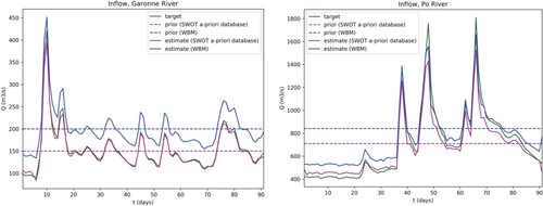
The inferred inflow discharge for this scenario are shown in purple on Figure 3 (Cases S1.Ga.σ and S1.Po.σ in Table 2). For each of the two rivers, the true daily inflow hydrograph over 90 days (green curve) is satisfactorily retrieved with $rRMS{E}_Q=24.3\mathrm{\%}$ on the Po River the and $rRMS{E}_Q=9\mathrm{\%}$ on the Garonne River (resp. $8.5\mathrm{\%}$ and $4.8\mathrm{\%}$ with perfect observations). For a better reading, the results obtained for the bathymetry are indicated using the deviation from the trend $B^{\ast }$ (cf Table 4 and Figure 2). The estimated bathymetry $b_{1,..,N}$ is improved by the VDA process on the Garonne River (the prior $RMS{E}_{b^{\left(0\right)}}=0.39$ decreases to $RMS{E}_b=0.31$); it remains close to the first guess in the Po River case. Let us recall that the friction parameter K is model-equations-geometry dependent; its calibrated value compensates various modelling errors.

Figure 3. Inflow discharge (true=target, prior, inferred=estimate) with daily SWOT-like observations (ObsFs context). (Left) Garonne River cases S1.Ga.0.a/b (Right) Po River cases S1.Po.0.a/b

For these two ungauged experiments (Cases S1.Ga.σ; S1.Po.σ and S1.Ga.0; S1.Po.0 with perfect observations, see Table 4), the inference of discharge remains robust and accurate. Most of the identification errors are absorbed by the friction coefficient. It can be noticed that the equifinality issue between the bathymetry and the friction may be observed. Indeed, on the Po River while discharge is very well retrieved, neither the bathymetry nor the friction coefficient is significantly improved by the VDA process; different (friction, bathymetry) pair values can produce similar (correct) discharge values. This observation is consistent with the mathematical development presented in Section A.1. However this ‘optimal value’ of $(K,b(x\left)\right)$, solution of (10(10) $\underset{k}{min}\mathrm{J}\left(k\right)$(10) ), may be refined by solving afterwards the algebraic model presented in Section 8, see Table 4.

To illustrate the ill-posedness feature of the inverse problem (A.1) in Scenario S1), another experiment has been performed for the Garonne and the Po Rivers: the first guesses have been computed using either the WBM mean annual flow [50] (Cases S1.Ga.0.b, S1.Ga.σ, S1.Po.0.b and S1.Po.σ) or the mean discharge from the SWOT a-priori river database, see e.g. [48] (Cases S1.Ga.0.a, S1.Ga.σ, S1.Po.0.a and S1.Po.σ), see Table 3. For both rivers, the WBM mean annual flow provides a bad estimate of the average flow (on the calibration window) whereas the SWOT a-priori river database provides a good estimate. For instance for Garonne River the true average flow is $154{\mathrm{m}}^3{\mathrm{s}}^{-1}$; WBM mean annual flow provides $200{\mathrm{m}}^3{\mathrm{s}}^{-1}$ and SWOT river database provides $150{\mathrm{m}}^3{\mathrm{s}}^{-1}$.

Table 3. Scores of the inversions performed from different priors (‘a’ for SWOT a-priori database, ‘b’ for WBM) defining the hydrograph first guess $Q^{\left(0\right)}$; Scenario S1).

			$Q_{prior}$	$RMS{E}_{b^{\left(0\right)}}$	$RMS{E}_Q$	$rRMS{E}_Q$	$rRMS{E}_{Q\ast }$	$RMS{E}_b$
Case	River	${\sigma }_Z^{obs}$	$\left({\mathrm{m}}^3{\mathrm{s}}^{-1}\right)$	$\left(\mathrm{m}\right)$	$\left({\mathrm{m}}^3{\mathrm{s}}^{-1}\right)$	$\left(\mathrm{\%}\right)$	$\left(\mathrm{\%}\right)$	$\left(\mathrm{m}\right)$
S1.Ga.0.a	Garonne	0	150	0.18	13.4	5.1	5.0	0.43
S1.Ga.0.b	Garonne	0	200	0.51	40.6	30.5	7.5	0.73
S1.Ga.σ	Garonne	25 cm	150	0.39	24.0	10.3	9.8	0.31
S1.Ga.σ	Garonne	25 cm	200	0.54	41.8	33.0	13.3	0.45
S1.Po.0.a	Po	0	710	0.61	83.9	8.5	8.5	0.75
S1.Po.0.b	Po	0	841	0.91	88.4	17.1	11.0	0.92
S1.Po.σ	Po	25 cm	710	0.92	185.9	24.8	24.8	1.04
S1.Po.σ	Po	25 cm	841	1.12	235.3	31.5	24.9	1.24

Table 4. Scores of the inversions for the different cases.

				$RMS{E}_{b^{\left(0\right)}}$	$RMS{E}_Q$	$rRMS{E}_Q$	$RMS{E}_b$
Case	Scenario	River	${\sigma }_Z^{obs}$	$\left(\mathrm{m}\right)$	$\left({\mathrm{m}}^3{\mathrm{s}}^{-1}\right)$	$\left(\mathrm{\%}\right)$	$\left(\mathrm{m}\right)$
S1.Ga.0	S1)	Garonne	0	0.18	13.4	5.1	0.27
S1.Po.0	S1)	Po	0	0.61	83.9	8.5	0.75
S1.Ga.σ	S1)	Garonne	25 cm	0.39	24.0	10.3	0.31
S1.Po.σ	S1)	Po	25 cm	0.92	185.9	24.8	1.04
S2.Ga.0	S2)	Garonne	0	0.17	10.0	4.2	0.16
S2.Po.0	S2)	Po	0	0.73	91.2	10.2	0.88
S2.Ga.σ	S2)	Garonne	25 cm	0.42	17.9	8.5	0.38
S2.Po.σ	S2)	Po	25 cm	0.83	183.7	24.3	1.07
S3.Ga.0	S3)	Garonne	0	0.16	11.9	5.2	0.22
S3.Po.0	S3)	Po	0	0.48	76.4	7.8	0.45
S3.Ga.σ	S3)	Garonne	25 cm	0.35	19.4	9.1	0.27
S3.Po.σ	S3)	Po	25 cm	0.64	144.8	18.3	0.60
S1.Sa.0	S1)	Sacramento	0	2.29	30.1	11.5	2.33
S1.Sa.σ	S1)	Sacramento	34 cm	2.45	124.7	19.3	2.49
S3.Sa.0	S3)	Sacramento	0	1.95	54.5	15.9	2.01
S3.Sa.σ	S3)	Sacramento	34 cm	1.84	141.2	20.2	1.82

If measuring the inference accuracy in terms of rRMSE on Q, the results obtained for these 12 experiments show that poor priors $Q^{\left(0\right)}$ may lead to poor estimations of the discharge, see Table 4. For the case S1.Ga.0.a, $rRMS{E}_Q=5.1\mathrm{\%}$ ; this is better than in the case S1.Ga.0.b where $rRMS{E}_Q=30.5\mathrm{\%}$. For the case S1.Ga.σ, $rRMS{E}_Q=10.3\mathrm{\%}$ , and $rRMS{E}_Q=33.0\mathrm{\%}$ for the S1.Ga.σ.b case. The same remark can be made for the Po River.

However, as shown on Figure 3, the inferred temporal variations of Q remain excellent in all cases. Indeed, to better illustrate that the bias is fully dependent on the prior, an adapted value of rRMSE is computed from $Q^{\ast }(x,t)=\left({\overline{Q}}_{true}/{\overline{Q}}^{\left(0\right)}\right)Q(x,t)$ (i.e. normalized by the bias of the prior). In each case, the values of this metric obtained for the two sources of $Q^{\left(0\right)}$ are close: $rRMS{E}_{Q\ast }=7.5\mathrm{\%}$ (Case S1.Ga.0.b) and $rRMS{E}_{Q\ast }=5.0\mathrm{\%}$ (Case S1.Ga.0.a); $rRMS{E}_{Q\ast }=13.3\mathrm{\%}$ (Case S1.Ga.σ) and $rRMS{E}_{Q\ast }=9.8\mathrm{\%}$ (Case S1.Ga.σ); $rRMS{E}_{Q\ast }=11.0\mathrm{\%}$ (Case S1.Po.0.b) and $rRMS{E}_{Q\ast }=8.5\mathrm{\%}$ (Case S1.Po.0.a); $rRMS{E}_{Q\ast }=24.9\mathrm{\%}$ (Case S1.Po.σ) and $rRMS{E}_{Q\ast }=24.8\mathrm{\%}$ (Case S1.Po.σ).

This high accuracy of the discharge temporal variations is consistent with the mathematical formal proof presented in Section A.1.

On the equifinality issue & the importance of one ancillary data. These numerical results illustrate the ill-posedness features of the inverse problem if no additional in-situ data (e.g. accurate mean first guesses values) is considered, see Section A.1. Indeed the space-time variations of the inferred discharge are very accurate but they may present a bias, see Figure 3. The bias vanishes if the (scalar) prior value $Q^{\left(0\right)}$ is sufficiently accurate; $Q^{\left(0\right)}$ may be the mean value of Q. As a consequence if the a-priori value(s), see Section 5.2, are far from reality, the rRMSE criteria on the estimation may be large, see e.g. case S1.Ga.σ in Table 3. On the contrary the rRMSE computed from $Q^{\ast }(x,t)$ remains excellent, Figure 3. This bias can be explained by the re-scaling calculation presented in Section A.1.

6.2. Inferences for partially gauged rivers: Scenario S2)

Many worldwide rivers are not fully ungauged. In this section, relatively good priors of discharge are provided at one location in the river portion at each instant p; they are denoted by $(Q_1^g,\dots ,Q_P^g)$. These values may be provided by either a global discharge database or a calibrated hydrological model. Given such priors of discharge values, we compute corresponding values $(A_0^g,K^g)$ using an additional ‘low complexity flow model’: Equation (A1(A1) $c_{r,p}\cdot K_{r,p}^{3/5}{A}_{r,0}+d_{r,p}\cdot K_{r,p}^{3/5}=Q_{r,p}^{frac35}\text{for all }(r,p)$(A1) ), see also (A2(A2) $D_{c}Bil(\tilde{K},A)+D_d\tilde{K}=\tilde{Q}\text{ in }{R}^{R(P+1)}$(A2) ). These new systems are derived from (4(4) $(K_{r,p}^{-1}{Q}_{r,p}{)}^{3/5}=(A_{0,r}+\delta A_{r,p})W_{r,p}^{-2/5}{S}_{r,p}^{3/10}\mathrm{\forall }r,\mathrm{\forall }p$(4) ); their derivations are detailed in Appendix A.2.

Estimations of $(A_{r,0},K_{r,p}{)}_{R,P}$ given Q at one gauge station.

We consider the same value of discharge (in time) at each reach r; that is in Equation (A2(A2) $D_{c}Bil(\tilde{K},A)+D_d\tilde{K}=\tilde{Q}\text{ in }{R}^{R(P+1)}$(A2) ) we set: $\begin{array}{rl}\tilde{Q}& =\left(\left(\right(Q^g{)}_0^{3/5},\dots ,\left(Q^g{)}_0^{3/5}\right),\dots ,\left(\right(Q^g{)}_p^{3/5}\dots \left(Q^g{)}_p^{3/5}\right),\dots ,\left(\right(Q^g{)}_P^{3/5}\dots \left(Q^g{)}_P^{3/5}\right)\right)\\ & \in R^{R(P+1)}\end{array}$ Next given $\tilde{Q}$, the pairs $(K_{r,p},A_{r,0}{)}_{R,P}$ are computed as solution of (A2(A2) $D_{c}Bil(\tilde{K},A)+D_d\tilde{K}=\tilde{Q}\text{ in }{R}^{R(P+1)}$(A2) ). This provides a prior of bathymetry $(A_{r,0}{)}_R$. Concerning the friction, given the values $(K_{r,p}{)}_{R,P}$, either a uniform mean value $\overline{K}$ is considered or a uniform law is considered (that is ($\overline{\alpha },\overline{\text{β}}$), see (3(3) $K\left(h\right)=\alpha h^{\text{β}}$(3) )).

Results. The results obtained in Scenario S2) are a little bit more accurate than those obtained in Scenario S1), see Table 4. For the Garonne River, $rRMS{E}_Q=4.2\mathrm{\%}$ (Case S1.Ga.0) and $rRMS{E}_Q=8.5\mathrm{\%}$ (Case S1.Ga.σ). For the Po River, $rRMS{E}_Q=10.2\mathrm{\%}$ (Case S1.Po.0) and $rRMS{E}_Q=24.3\mathrm{\%}$ (Case S1.Po.σ).

This method can also be extended to the case where statistics on the discharges values are available (for instance quantiles or probability density functions).

In this latter case, the system must be employed with the corresponding statistics on flow lines. For instance if percentiles $(Q_m{)}_M$ are given where $Q_m$ is m-th percentile of discharge, the system must be solved using observations corresponding the same quantiles of flow lines.

6.3. Inferences with one bathymetry measurement available: Scenario S3)

In Scenario S3), the in-situ measurement of the bathymetry at one location $b_{ref}$ enables estimation of the so-called low Froude bathymetry, see Equation (5(5) $b_r+(Z_{ref,p}-b_{ref})\cdot {\mathcal{O}}_{ref,p}^{-1}\cdot {\mathcal{O}}_{r,p}=Z_{r,p}\mathrm{\forall }r,r\ne ref,\mathrm{\forall }p\ge 0$(5) ) and Section 5.2. This estimation is employed as the first guess bathymetry $b^{\left(0\right)}$ ins the VDA process, see (6(6) $c={\left(Q_{in,0},\dots ,Q_{in,P};b_1,\dots ,b_N;\alpha ,\text{β}\right)}^T$(6) ).

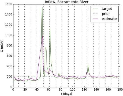
As already pointed out this bathymetry estimation presents an increasing drift with the distance to the reference measurement location $x_{ref}$. Indeed, the equation is a first order differential equation. In the Sacramento river case, a segmentation in two parts had to be done; each part corresponding to one reference bathymetry value, see Figure 2 (Bottom Right).

The numerical results presented on Figure 4 correspond to the inferences of $(Q_{in,1},..,Q_{in,P};b_1,..,b_N;\alpha ,\text{β})$ obtained by VDA with the first guesses $(Q^{\left(0\right)};b^{\left(0\right)};{\alpha }^{\left(0\right)},{\text{β}}^{\left(0\right)})$ defined as Scenario S3) in Section 5.2. (Note that here $(\alpha ,\text{β})$ are constant values).

Figure 4. Inflow discharge with the bathymetry priors inferred using the Low-Froude model and one (1) in-situ point ($b^0$ ‘Low Froude’). Daily SWOT-like observations (ObsFs context), noise ${\sigma }_Z=0.25$ (a, b).

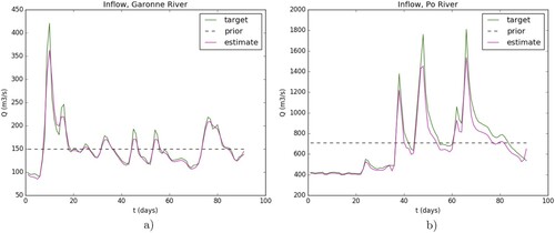
In terms of bathymetry, Scenario S3) provide better estimations for the first guess (see Table 4). This is particularly true for the Po river with $RMS{E}_{b^{\left(0\right)}}=0.61\mathrm{m}$ for the S1.Po.0 case and $RMS{E}_b=0.48\mathrm{m}$ for the S3.Po.0 case. For the Garonne River the improvement is negligible because Scenario S1) already provides good prior of bathymetry. One can notice that the prior values are even better than the inferred values in Scenario S1). It should also be noticed that the VDA does not update much the bathymetry. As a consequence the first guess can be used as is to infer $(Q_{in,1},..,Q_{in,P};K)$ only. We recall that the inference of $(Q_{in,1},..,Q_{in,P};K)$ only is much more robust.

However, Scenario S3) does not bring significant improvement on discharge when compared to Scenario S2). For the Garonne River $rRMS{E}_Q=5.2\mathrm{\%}$ (Case S3.Ga.0) and $rRMS{E}_Q=5.2\mathrm{\%}$ (Case S3.Ga.σ); these results are close to those obtained for Scenario S2) (or even Scenario S1 with a good prior). For the Po River $rRMS{E}_Q=7.8\mathrm{\%}$ (Case S3.Po.0) and $rRMS{E}_Q=18.3\mathrm{\%}$ (Case S3.Po.σ); for this river, Scenario S3) slightly outperforms Scenario S2), especially for the case with noise. For the Sacramento River $rRMS{E}_Q=15.9\mathrm{\%}$ (Case S3.Sa.0) and $rRMS{E}_Q=20.2\mathrm{\%}$ (Case S3.Sa.σ); for the case with perfect observations, results in Scenario S3) are even slightly worse than results in Scenario S2). This is in good agreement with the results presented in Appendix A.1 that a good prior for either Q, K or b is sufficient to improve the accuracy of the inferred values.

7. Inferences in ObsNs context: Sacramento river

This section presents the numerical inference of the complete control vector (6(6) $c={\left(Q_{in,0},\dots ,Q_{in,P};b_1,\dots ,b_N;\alpha ,\text{β}\right)}^T$(6) ) in the 1D Saint-Venant model (1(1) $\begin{array}{rl}{\mathrm{\partial }}_{t}A+{\mathrm{\partial }}_{x}Q& =0\\ {\mathrm{\partial }}_{t}Q+{\mathrm{\partial }}_x\left(\frac{Q^2}{A}\right)+gA{\mathrm{\partial }}_{x}Z& =-gA{S}_f(A,Q;K)\end{array}$(1) ) with SWOT Nominal (ObsNs) sampling for the Sacramento River. In this context, that frequency of observations is low when compared to the hydrograph frequencies.

7.1. Identifiability map and preliminary analysis

The discharge inference capabilities depend on the space-time sampling of the observations and on the flow dynamics. An instructive reading of the inverse problem can be obtained by plotting the ‘identifiability map’ introduced in [28]. The identifiability map represents the complete information in the $(x,t)$-plane: the ‘space-time windows’ observed by SWOT, the hydrodynamic wave propagation (flow model in fluvial regime) and the misfit to the ‘local equilibrium’ (local misfit between the steady-state uniform flow and the dynamic flow). We refer to [28] for more details. This preliminary analysis enables to roughly estimate the inflow time intervals that can be identified by the VDA process. Indeed the inflow discharge mathematically arises from these observed ‘space-time windows’. This qualitative reading of the inverse problem is instructive because it enables to estimate if the unknown information has been indirectly measured or not. In the present case (Sacramento River case), the reach of 147 km long is completely observed by two satellite tracks respectively at the 9th and 19th days (for each 21 days repeat period). As the Sacramento River is considered ungauged in this experiment, the exact identifiability map cannot be computed. To circumvent this point, an a-priori identifiability map is computed as follows:

• A VDA inference of the control vector c is performed (based on Scenario S1)).

• Given the optimal control vector c, the (forward) Saint-Venant flow model (1(1) $\begin{array}{rl}{\mathrm{\partial }}_{t}A+{\mathrm{\partial }}_{x}Q& =0\\ {\mathrm{\partial }}_{t}Q+{\mathrm{\partial }}_x\left(\frac{Q^2}{A}\right)+gA{\mathrm{\partial }}_{x}Z& =-gA{S}_f(A,Q;K)\end{array}$(1) ) is re-runned.

• The ‘equilibrium misfit’ $\mid S_g-S_f\mid$, $S_g={\mathrm{\partial }}_{x}Z$ (see Equations (1(1) $\begin{array}{rl}{\mathrm{\partial }}_{t}A+{\mathrm{\partial }}_{x}Q& =0\\ {\mathrm{\partial }}_{t}Q+{\mathrm{\partial }}_x\left(\frac{Q^2}{A}\right)+gA{\mathrm{\partial }}_{x}Z& =-gA{S}_f(A,Q;K)\end{array}$(1) ) and [28] for details) and the wave propagation times ($T_{wave}$) are computed from the forward flow model outputs.

The obtained identifiability map is plotted on Figure 5. Due to the observation layover, there are few unobserved zones for the second SWOT pass, for example at x = 80 km and t = 19, 40 and 61 days. Given the WS observation of each reach at a given time, the purple dots at x = 0 (upstream BC) on Figure 5 represent the origin of the characteristics. In other words they represent the hydraulic information propagation at inflow. Following this analysis, the identifiability of $Q_{in}\left(t\right)$ is possible on time windows of ∼2 days (∼40h for the flood peak recession at day 51) before observation times.

Figure 5. Identifiability map. Overview in the $(x,t)$-plane of the inverse problem features: observables, hydraulic wave speed and ‘equilibrium misfit’ (colours bar) (= the non-conservative part of the momentum Equation (1(1) $\begin{array}{rl}{\mathrm{\partial }}_{t}A+{\mathrm{\partial }}_{x}Q& =0\\ {\mathrm{\partial }}_{t}Q+{\mathrm{\partial }}_x\left(\frac{Q^2}{A}\right)+gA{\mathrm{\partial }}_{x}Z& =-gA{S}_f(A,Q;K)\end{array}$(1) )b). For each observation of the domain, the vertical spreading corresponds to the time $\alpha \cdot \mathrm{\Delta }x/u$ necessary for the upstream wave to cross an observed cell of size $\mathrm{\Delta }x$ (α is a dilatation factor for sake of readability only). (Left) The complete $(x,t)$-plane. (Right) Zoom on the most varying time interval. .

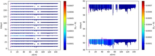
The ‘equilibrium misfit’ $\mid S_g-S_f\mid$ is represented on the map; it highlights where and when the flow is not locally stationary-uniform. The magnitude of this equilibrium misfit increases where and when a flood wave is travelling through the domain; see observations at day 51 and day 61 on Figure 5 and 6. The identifiability map analysis shows that the WS deformations due to the flood peak between days 51 and 61 have not been observed. Also this analysis indicates that the mean information propagation time throughout the domain equals ∼40 h.

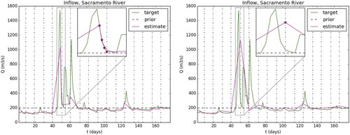
Figure 6. Inflow discharge (target=true, prior and inferred=estimate) with SWOT-HR observations (ObsNs context), Sacramento River, case S1.Sa.0. Computations with 4 assimilation points every (0, 12, 24, and $36\mathrm{h}$) before observation times (a) or at observation times only (b).

Based on the purple dots at x = 0 (upstream BC) (see the explanation of their meaning above), we define 3 additional assimilation points every $\approx 12$h before the observation days 51 and 61. Indeed these additional assimilation instants contain information on the first flood peak recession and the third flood peak rise respectively.

7.2. Inferences in Scenario S1)

The identifiability maps has provided some crucial information to set up the VDA process.

The inflow discharge, bathymetry and friction inferred by VDA are shown respectively on Figure 6(a) and Table 4.

The discharge identification is accurate at each observation time and for the 3 points preceding the observed flood peaks at t = 51 and 61 days. It is worth noticing that a basic approach consisting in infering discharge at observation times only would lead to a less accurate hydrograph inference as shown in Figure 6(b).

The flood peak between days 51 and 61 is not retrieved since the peak effects have not been observed; this is consistent with the preliminary identifiability map analysis, see Section 7.1.

Following [28], the identifiability index $I_{ident}=T_{wave}/\mathrm{\Delta }{t}_{obs}$ is evaluated for a wave propagation time ($T_{wave}$) of about $72h$ (with $\mathrm{\Delta }{t}_{obs}\sim 10$ days). This results to $I_{ident}\sim 0.3$, that is a relatively low identifiability index (see [28], for details). Interestingly, even with this low identifiability value, the inference of discharge is accurate at observation instants but also at the ‘identifiable instants’ defined before flood observations thanks to the identifiability map analysis.

The discharge values are accurately inferred with $rRMS{E}_Q=11.5\mathrm{\%}$ (Case S1.Sa.0) and $rRMS{E}_Q=19.3\mathrm{\%}$ (Case S1.Sa.σ). To obtain such good results it is mandatory to use the identifiability map. Indeed the discharge values when inferred at observation instants (Figure 6(b)) only is $rRMS{E}_Q=47.2\mathrm{\%}$ (Figure 7).

Finally we point out that the inferred discharge is accurate while the bathymetry and friction need to be refined using other information or equations; this is done in next section using the low complexity systems presented in Section 2.3.

7.3. Inferences in Scenario S3)

As stated in Section 5.3, to overcome the drift in space inherent in Equation (5(5) $b_r+(Z_{ref,p}-b_{ref})\cdot {\mathcal{O}}_{ref,p}^{-1}\cdot {\mathcal{O}}_{r,p}=Z_{r,p}\mathrm{\forall }r,r\ne ref,\mathrm{\forall }p\ge 0$(5) ), a segmentation in two parts of the Sacramento river has been done and two reference bathymetry values are used, see Figure 2 (Bottom Right). This allows to obtain better prior for the bathymetry than for Scenario S1 with $RMS{E}_{b^{\left(0\right)}}=1.95$ m for the S3.Sa.0 case and $RMS{E}_b=1.84$ m for the S3.Sa.σ case. However in terms of accuracy of the inferred discharge, the results obtained are slightly worse than those obtained in Scenario S1, with $RMS{E}_Q=15.9\mathrm{\%}$ for the S3.Sa.0 case and $RMS{E}_Q=20.2\mathrm{\%}$ for the S3.Sa.σ case. Final, one can notice that like in the ObsFs context, the VDA those not vary much the bathymetry.

Figure 7. Inflow discharge with the bathymetry priors inferred using the Low-Froude model and one (1) in-situ point ($b^{\left(0\right)}$ ‘Low Froude’). SWOT-HR observations (ObsNs context), Sacramento River.

8. Past the calibration - ‘learning’ period: real computational time estimations of Q

The inversion method previously presented is based on VDA and WS measurements. This approach may be summarized as least-square estimations fitting the WS measurements (and potentially prior values too). It is highly advisable to perform it on a complete hydrological cycle (12 months minimum) presenting a large range of variability (from low to high flow lines, discharge values). The VDA method cannot be performed in real-time. In this section, a strategy to estimate discharge values in real-time is proposed.

The estimations obtained by VDA (as previously described) are performed on a sufficiently varying measurements dataset : it is the so-called ‘calibration’ -- ‘learning’ period. As a result, relatively accurate values of $\left(A_{r,0}\right)\in R^R$ and $\left(Q_{r,p}\right)\in R^{R(P+1)}$ are obtained. Given these $(Q_{r,p},A_{r,0}{)}_{R,P}$ values, an effective space-time dependent friction coefficient $(K_{r,p}{)}_{R,P}$ corresponding to the Low-Froude algebraic flow model (A2(A2) $D_{c}Bil(\tilde{K},A)+D_d\tilde{K}=\tilde{Q}\text{ in }{R}^{R(P+1)}$(A2) ) can be straightforwardly computed. Recall that the friction parameter K is fully model dependent; it is not an intrinsic feature of the flows.

In other respects, this low Froude algebraic system is relatively accurate : it has been throughly assessed in the present cases (see Figure 8 with the upcoming estimations too). Moreover it can be solved in real-time ($0.3s/cycle$ on standard laptop).

Figure 8. Discharge estimations obtained from System (A2(A2) $D_{c}Bil(\tilde{K},A)+D_d\tilde{K}=\tilde{Q}\text{ in }{R}^{R(P+1)}$(A2) ) (after re-calibration of the friction K). Plot: $Q_{target}$ (see Table 5) vs $Q_{inferred}$. (Top). Discharge Garonne River; (Bottom) Po River. (Left) With $K\left(h\right)$ hence $K_p$; (Right) With ${\overline{K}}_r$.

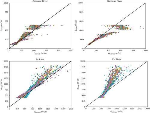
Table 5. Observations sources and characteristics for each test river.

River	Hydrodynamic	Temporal	#nodes	#reaches	Observations
	model	window	(N)	(R)	context
Garonne [46]	HEC-RAS	06 Jan. 2010−06 Apr. 2010	376	75	ObsFs
Po [47]	HEC-RAS	01 Jan. 2002−01 Apr. 2002	488	97	ObsFs
Sacramento	HEC-RAS + SWOT HR	01 Jan. 2009−27 Jun. 2009	718	17	ObsNs

Therefore given new observations $(Z_r,W_r{)}_{1,..,R}$ (satellite observations acquired past the ‘learning period’), the discharge values $(Q_r{)}_{1,..,R}$ can be computed in real-time simply by evaluating in real-time System (A2(A2) $D_{c}Bil(\tilde{K},A)+D_d\tilde{K}=\tilde{Q}\text{ in }{R}^{R(P+1)}$(A2) ) (see also (4(4) $(K_{r,p}^{-1}{Q}_{r,p}{)}^{3/5}=(A_{0,r}+\delta A_{r,p})W_{r,p}^{-2/5}{S}_{r,p}^{3/10}\mathrm{\forall }r,\mathrm{\forall }p$(4) )). Below numerical results illustrate such real-time estimations.

8.1. Friction coefficient re-calibration

Given $(Q_{r,p},A_{r,0}{)}_{R,P}$ obtained by the VDA process, a new (effective) friction coefficient corresponding to the low Froude -- low complexity flow model is computed : this is the ‘re-calibration’ step of K. Space-time dependent values $K_{r,p}$ are obtained by solving (A2(A2) $D_{c}Bil(\tilde{K},A)+D_d\tilde{K}=\tilde{Q}\text{ in }{R}^{R(P+1)}$(A2) ). Next one of the two methods below are employed:

1)	For each reach r, a mean value is considered as: ${\overline{K}}_r=mea{n}_p\left(K_{r,p}\right)$. This mean value is computed on a subset of the WS observations e.g. by considering the interval [2nd - 8th] deciles of the flow profiles (20 overpasses were selected in this study). (This choice corresponds to a relatively wide and representative range of flow regimes without the extremes).
2)	For each reach r, a power law is considered as: $K_r\left(h\right)={\alpha }_r{h}^{{\text{β}}_r}$. To do so, given the water depth $h_{r,p}$, $h_{r,p}=(Z_{r,p}-b_r)$ with $b_r$ the inferred values, $({\alpha }_r,{\text{β}}_r)$ are computed as the optimal values in the least-square sense.

The case of Sacramento River is not considered in this section because the number of observations is not sufficient to select reliable deciles of the flow profiles. The re-calibration methods above are adequate to the present cases (Garonne and Po rivers) because no over-bank flow occurs.

The present experiments correspond to a calibration period of 90 days (the VDA inversions are obtained on this dataset), and a validation period (real-time estimations) of $\sim 9$ months.

8.2. Estimations of Q in real-time

Given the re-calibrated friction coefficients $\left(K_r\right(h){)}_{\mathrm{1..}R}$, the discharge is computed by solving System (A2(A2) $D_{c}Bil(\tilde{K},A)+D_d\tilde{K}=\tilde{Q}\text{ in }{R}^{R(P+1)}$(A2) ) with its coefficients provided by the newly acquired WS measurements (validation period of $\sim 9$ months). The obtained values in the case of the Po and Garonne Rivers (with all flow lines) are plotted on Figure 8.

For both rivers, using a friction coefficient ${\overline{K}}_r$ constant in time provides the best results. The resulting errors are: $rRMS{E}_Q=6.3\mathrm{\%}$ for the Garonne River and $rRMS{E}_Q=10.6\mathrm{\%}$ for the Po River. Note that these performances are evaluated at all observation times and all R reaches whereas for the VDA inference (Sections 6 and 7) the performances are evaluated at upstream only i.e. for r = 0.

The second method for re-calibrating the friction coefficients $K_r\left(h\right)$ provides lower accurate results but they remain acceptable; the errors are: $rRMS{E}_Q=9.1\mathrm{\%}$ for the Garonne River and $rRMS{E}_Q=25.3\mathrm{\%}$ for the Po River. Recall that the flow model is calibrated from the observed flow lines hence presenting a minimal and a maximal WS elevation. The re-calibrated friction coefficient K is related to this flow lines range. If K is defined as a power law $K_r\left(h\right)$ and if the newly acquired WS elevation is greater than the previously observed WS than the friction power law is prone to an over-estimation. That is the reason why we encourage to prefer the first method (considering ${\overline{K}}_r$) to the second one (power law).

In conclusion, solving the dedicated low-complexity algebraic system (A2(A2) $D_{c}Bil(\tilde{K},A)+D_d\tilde{K}=\tilde{Q}\text{ in }{R}^{R(P+1)}$(A2) ), after re-calibration of the friction parameter K constitutes a promising method to estimate the discharge in real-time that is in an operational way. (It is actually a ‘computational real time’ given the newly acquired data; indeed the satellite data may be provided with latency).

9. Conclusion

This study proposes a new hierarchical computational inversion method to infer the discharge $Q\left(t\right)$, an effective bathymetry $b\left(x\right)$ with a corresponding friction coefficient K from altimetry Water Surface (WS) measurements, more specifically data from the upcoming SWOT satellite [1]. The inversion method is based on a combination of an advanced Variational Data Assimilation (VDA) formulation applied to the classical Saint-Venant equations (1D shallow-water) and original algebraic systems (low-Froude, locally permanent flows). The VDA formulation takes into account adequate scale dependency and a-priori error measurement amplitudes.

The algebraic systems natively integrate the measured quantities; they may be differently employed depending on the fields that are not known. They enable to exploit in a consistent manner databases to define the first guesses (prior information) of the iterative VDA process. Moreover they enable to compute in real-time the discharge past the ‘calibration-learning period’ (i.e. the assimilation of a complete hydrological year dataset).

Three rivers, $\sim 100$ km long each, have been considered with two contexts of observation: the SWOT Cal-Val orbit with (ObsFs context) ∼ 1 day period (or any equivalent multiple-sensor measurements) and SWOT like nominal sampling (ObsNs context) with $\sim 21$ days period (with 1 to 4 passes at mid-latitudes). The corresponding inversions are highly challenging since relying on relatively sparse observations (both in space and time) compared to the potential flow dynamics. Indeed the flows present low identifiability indexes as defined in [28]. Preliminary analyses based on the identifiability maps introduced in [28] enable to define adequate time grids for the identification process.

For ungauged rivers and/or in total absence of good prior information on the flow (rough estimation of the mean annual flow only), the inversion algorithm provides accurate space-time variations of Q with an effective bathymetry $b\left(x\right)$ and a corresponding friction coefficient $K\left(h\right)$ (K function of the water depth h). However if the prior mean value of one of the three inferred fields (typically those of Q) is far from reality, a bias on the inferred hydrograph $Q\left(t\right)$ may remain. But as soon as a good mean value is provided (e.g. a mean discharge value from a database or from a large scale hydrological model), or a single reference value of bathymetry, the bias vanishes: the discharge $Q\left(t\right)$ is perfectly recovered even in terms of amplitudes (RMSE of a few percent at observation times are obtained).

Past the calibration period by VDA, the estimated values of $Q\left(t\right)$ and $b\left(x\right)$ obtained by the VDA process are kept and a new (effective) friction coefficient $K\left(x\right)$ corresponding to the low complexity flow model is computed. Next, this low complexity (algebraic) model can provide estimations of the discharge Q in real-time from newly acquired satellite data.

This new and complete inverse method fulfils the conditions of an operational solution to the estimations of rivers discharge at global scale from the upcoming SWOT satellite mission (launch planned in 2021).

All the present equations and algorithms have been implemented into the open-source computational software DassFlow [33]. The present algorithms and computation al code have been recently employed with multi-satellite datasets (ENVISAT, SWOT) for a braided river, [51]. Moreover investigations are in progress for larger rivers presenting lateral fluxes.

Acknowledgments

The authors K. Larnier (software engineer at CS corp.) and J. Verley have been funded by CNES. The authors acknowledge: M. Durand from Ohio State University for providing the Sacramento SWOT-HR dataset; H. Roux from IMFT / INPT Toulouse for providing an expertise on the Garonne River dataset. The authors acknowledge anonymous reviewers for their helpful comments. The corresponding author has derived the equations and built up the computational methods; he has written the majority of the manuscript. The first author has performed all the presented numerical results (plus many exploring ones), after having greatly enriched the computational software DassFlow1D from the previous version developed by P. Brisset [28]. The third author has contributed to the model setups on real datasets and their analysis; he has suggested the sensitivity to densified temporal identifiability. The last author has nicely contributed to the VDA formulation during the beginning of his PhD.

Disclosure statement

No potential conflict of interest was reported by the author(s).

Additional information

Funding

The authors K. Larnier (software engineer at CS corp.) and J. Verley have been funded by CNES.

Appendix

A.1. On the potentially ill-posed inverse problem

In this paragraph we show that the inverse problem based on the 1D Saint-Venant Equations (1(1) $\begin{array}{rl}{\mathrm{\partial }}_{t}A+{\mathrm{\partial }}_{x}Q& =0\\ {\mathrm{\partial }}_{t}Q+{\mathrm{\partial }}_x\left(\frac{Q^2}{A}\right)+gA{\mathrm{\partial }}_{x}Z& =-gA{S}_f(A,Q;K)\end{array}$(1) ) and the WS data only (no additional in-situ data is available even not a mean value) is ill-posed in the sense its solution is defined to a multiplicative factor. This feature is confirmed in numerical results (Section 6).

Let $\overline{\alpha }$ be a scalar value. Typically $\overline{\alpha }$ is a mean value of K or Q. Let us re-scale the variables $(A,Q,h)$ as follows: $(A_{\ast },Q_{\ast },h_{\ast })=(A,Q,h)/\overline{\alpha }$ with e.g. the cross-section shape relation $A_{\ast }=h_{\ast }W$, W the measured surface width (or any linear combination of super-imposed trapeziums).

The mass equation divided by $\overline{\alpha }$ reads: ${\mathrm{\partial }}_t\left(A_{\ast }\right)+{\mathrm{\partial }}_x\left(Q_{\ast }\right)=0$. Therefore as it is well known, in terms of mass, re-scaling Q implies to re-scale A by the same factor (or re-scaling equivalently the water depth h).

The momentum equation divided by $\overline{\alpha }$ reads: ${\mathrm{\partial }}_t\left(Q_{\ast }\right)+{\mathrm{\partial }}_x\left(\frac{Q_{\ast }^2}{A_{\ast }}\right)+g{A}_{\ast }{\mathrm{\partial }}_{x}Z=-g{A}_{\ast }{S}_f$ with $S_f$ the RHS previously defined: $S_f(A,Q;h;K)=\left(1/K^2\right)\left(|Q|Q/A^2{h}^{4/3}\right)$. A short calculation shows that: $S_f(A,Q,h;K)=S_f(A_{\ast },Q_{\ast },h_{\ast };{\overline{\alpha }}^{-2/3}K)$.At boundaries, both the imposed discharge at upstream and the normal depth at downstream are similarly re-scaled.Therefore, given the WS measurements $(W,Z)$, the 1D Saint-Venant equations (1(1) $\begin{array}{rl}{\mathrm{\partial }}_{t}A+{\mathrm{\partial }}_{x}Q& =0\\ {\mathrm{\partial }}_{t}Q+{\mathrm{\partial }}_x\left(\frac{Q^2}{A}\right)+gA{\mathrm{\partial }}_{x}Z& =-gA{S}_f(A,Q;K)\end{array}$(1) ) with friction coefficient K is equivalent to the same equations with the re-scaled variables $(A_{\ast },Q_{\ast },h_{\ast })$ but with the friction coefficient equal to $\left({\overline{\alpha }}^{-2/3}K\right)$.

As a consequence the inferred solution $(A,Q;K)$ obtained by inverting the Saint-Venant model (with inflow-outflow ungauged boundary conditions) is the solution corresponding to the given prior value $c_{prior}$, see (7(7) $j\left(c\right)=j_{obs}\left(c\right)+\gamma j_{reg}\left(c\right)$(7) )–(10(10) $\underset{k}{min}\mathrm{J}\left(k\right)$(10) ). (Recall that this prior value $c_{prior}$ is related to the first-guess value, see Section 5.2 for details).

This ill-posedness feature of the considered inverse problem (if no additional in-situ data or good prior values is introduced) is observed in the numerical results, see Section 6.

Observe that if imposing a rating curve at outflow e.g. $Q_{o}ut=cst{h}^{\gamma }$, then the re-scaled form of the law is not equivalent to the original one (excepted if $\gamma =1$). In other words, if imposing an accurate rating curve at outflow, the whole upstream flow is accurately controlled. (This statement valid for low Froude flows is classical). Moreover this highly controlling boundary condition cannot be re-scaled like the other model terms. However in practice such rating curve is unknown for ungauged rivers.

The same inversions based on the (scalar) Manning–Strickler equation or on the algebraic system (4(4) $(K_{r,p}^{-1}{Q}_{r,p}{)}^{3/5}=(A_{0,r}+\delta A_{r,p})W_{r,p}^{-2/5}{S}_{r,p}^{3/10}\mathrm{\forall }r,\mathrm{\forall }p$(4) ) (and not on the dynamic Saint-Venant equations) present equifinality issues even stiffer. Indeed, given a set of WS measurements $(Z_{r,p},W_{r,p}{)}_{R,P+1}$ and an effective low flow bathymetry $A_{0,r}\mathrm{\forall }r$ (therefore the effective cross-sectional area $A_{r,p}=A_{r,0}+\delta A_{r,p}\mathrm{\forall }r\in \left[\mathrm{1..}R\right]$ is given), the inference of the ratio $Q_{r,p}/K_{r,p}$ is possible from (4(4) $(K_{r,p}^{-1}{Q}_{r,p}{)}^{3/5}=(A_{0,r}+\delta A_{r,p})W_{r,p}^{-2/5}{S}_{r,p}^{3/10}\mathrm{\forall }r,\mathrm{\forall }p$(4) ) but not the pair $(Q_{r,p},K_{r,p})\dots$ Infering the discharge value from the WS measurements and local Manning–Strickler's laws i.e. the low Froude system (4(4) $(K_{r,p}^{-1}{Q}_{r,p}{)}^{3/5}=(A_{0,r}+\delta A_{r,p})W_{r,p}^{-2/5}{S}_{r,p}^{3/10}\mathrm{\forall }r,\mathrm{\forall }p$(4) ), requires additional information on the friction coefficient; otherwise the uncertainty on the estimation Q is proportional to the uncertainty on $K^{-1}$, and reciprocally.

A.2. Bilinear system in variables $(A_{r,0},K_{r,p}{)}_{R,P}$ and $(Q_{r,p}{)}_{R,P}$

In this paragraph we derive additional equations from the low complexity algebraic flow model (4(4) $(K_{r,p}^{-1}{Q}_{r,p}{)}^{3/5}=(A_{0,r}+\delta A_{r,p})W_{r,p}^{-2/5}{S}_{r,p}^{3/10}\mathrm{\forall }r,\mathrm{\forall }p$(4) ). These equations are employed for two different purposes:

• to compute priors values of $(A_{r,0},K_{r,p})$ given prior discharge values $Q_{r,p}$. (This is useful in Scenario 2), see Section 6.2).

• to compute values of $K_{r,p}$ consistent with the low Froude flow model in the real-time computation stage, see Section 8.1.

Let us assume that the friction varies both in space and time, that is $(K_{r,p}{)}_{R,P}$. Then (4(4) $(K_{r,p}^{-1}{Q}_{r,p}{)}^{3/5}=(A_{0,r}+\delta A_{r,p})W_{r,p}^{-2/5}{S}_{r,p}^{3/10}\mathrm{\forall }r,\mathrm{\forall }p$(4) ) reads as follows: (A1) $c_{r,p}\cdot K_{r,p}^{3/5}{A}_{r,0}+d_{r,p}\cdot K_{r,p}^{3/5}=Q_{r,p}^{frac35}\text{for all }(r,p)$(A1) with $c_{r,p}=W_{r,p}^{-2/5}{S}_{r,p}^{3/10}$ and $d_{r,p}=c_{r,p}\delta A_{r,p}$.

The coefficients $(c_{r,p}$ $,d_{r,p})$ can be evaluated from the altimetry measurements. System (A1(A1) $c_{r,p}\cdot K_{r,p}^{3/5}{A}_{r,0}+d_{r,p}\cdot K_{r,p}^{3/5}=Q_{r,p}^{frac35}\text{for all }(r,p)$(A1) ) is multi-linear in $(K_{r,p}^{3/5}{A}_{r,0},K_{r,p}^{3/5},Q_{r,p}^{3/5})$. It contains $R(P+1)$ equations. It can be employed differently depending on the available information and the unknowns. If considering the full set of unknowns $(K_{r,p}^{3/5},A_{r,0},Q_{r,p})$, it is an underdetermined system since it has $R\left(2\right(P+1)+1)$ unknowns; therefore in this case it cannot be solved since it has an infinity of solutions.

Let us define the diagonal matrices $D_c$ and $D_d$ of dimensions $\left[R\right(P+1){]}^2$ by: $M_c=diag\left(c_{r,p}\right)$, $M_d=diag\left(d_{r,p}\right)$. Let us define the vectors : $\tilde{K}=(K_{r,p}^{3/5}{)}_{r,p}\in R^{R(P+1)}$, $A=(A_{r,0}{)}_{r,}\in R^R$ and $\tilde{Q}=(Q_{r,p}^{3/5}{)}_{r,p}\in R^{R(P+1)}$. Then (A1(A1) $c_{r,p}\cdot K_{r,p}^{3/5}{A}_{r,0}+d_{r,p}\cdot K_{r,p}^{3/5}=Q_{r,p}^{frac35}\text{for all }(r,p)$(A1) ) reads: (A2) $D_{c}Bil(\tilde{K},A)+D_d\tilde{K}=\tilde{Q}\text{ in }{R}^{R(P+1)}$(A2) with the bilinear operator $Bil(\tilde{K},A{)}_{r,p}=K_{r,p}^{3/5}{A}_{r,0}\mathrm{\forall }r\mathrm{\forall }p$.

If $\tilde{Q}$ is given then (A2(A2) $D_{c}Bil(\tilde{K},A)+D_d\tilde{K}=\tilde{Q}\text{ in }{R}^{R(P+1)}$(A2) ) has $(P+2)R$ unknowns (the two vectors $\tilde{K}$ and A).

Remark A.1

For K constant in space but varying in time (e.g. K is defined as a power law in h) then $\tilde{K}=(K_p^{3/5}{)}_p\in R^{(P+1)}$. In this case, the $(P+1+R)$ unknowns $(K_p^{3/5},A_{r,0})$ can be computed by solving the overdetermined bilinear system (A2(A2) $D_{c}Bil(\tilde{K},A)+D_d\tilde{K}=\tilde{Q}\text{ in }{R}^{R(P+1)}$(A2) ) e.g. by employing a trusted region reflective algorithm.For K constant in time but varying in space, $\tilde{K}=(K_r^{3/5}{)}_r\in R^R$, the system (A2(A2) $D_{c}Bil(\tilde{K},A)+D_d\tilde{K}=\tilde{Q}\text{ in }{R}^{R(P+1)}$(A2) ) has $2R$ unknowns. Therefore if $P\ge 1$ (more than 2 overpasses), the solution $(K_r^{3/5},A_{r,0})$ can be computed e.g. by a trusted region reflective algorithm.

Remark A.2

Given large scale estimations of $Q=\left(Q_{r,p}\right)\in R^{R(P+1)}$ from hydrological models,  (A2(A2) $D_{c}Bil(\tilde{K},A)+D_d\tilde{K}=\tilde{Q}\text{ in }{R}^{R(P+1)}$(A2) ) may provide effective unobserved wetted areas $(A_{r,0}{)}_r$.

References

- Rodríguez E. Swot science requirements document. JPL document, JPL. 2012.
- Calmant S, Cretaux JF, Remy F. Principles of radar satellite altimetry for application on inland waters. In: Baghdadi N, Zribi M, editors. Microwave remote sensing of land surface. Elsevier; 2016. p. 175–218.
- Biancamaria S, Lettenmaier DP, Pavelsky TM. The swot mission and its capabilities for land hydrology. Surv Geophys. 2016;37(2):307–337. doi: 10.1007/s10712-015-9346-y
- Chow V. Handbook of applied hydrology. New York: McGraw-Hill Book; 1964. 1467.
- Bjerklie DM. Estimating the bankfull velocity and discharge for rivers using remotely sensed river morphology information. J Hydrol (Amst). 2007;341(3):144–155. doi: 10.1016/j.jhydrol.2007.04.011
- Durand M, Neal J, Rodríguez E, et al. Estimating reach-averaged discharge for the river severn from measurements of river water surface elevation and slope. J Hydrol (Amst). 2014;511:92–104. doi: 10.1016/j.jhydrol.2013.12.050
- Garambois PA, Monnier J. Inference of effective river properties from remotely sensed observations of water surface. Adv Water Resour. 2015;79:103–120. doi: 10.1016/j.advwatres.2015.02.007
- Yoon Y, Garambois PA, Paiva R, et al. Improved error estimates of a discharge algorithm for remotely sensed river measurements: test cases on Sacramento and Garonne Rivers. Water Resour Res. 2016;52(1):278–294. doi: 10.1002/2015WR017319
- Durand M, Gleason C, Garambois PA. An intercomparison of remote sensing river discharge estimation algorithms from measurements of river height, width, and slope. Water Resour Res. 2016;52(6):4527–4549. doi: 10.1002/2015WR018434
- Roux H, Dartus D. Use of parameter optimization to estimate a flood wave: potential applications to remote sensing of rivers. J of Hydrology. 2006;328:258–266. doi: 10.1016/j.jhydrol.2005.12.025
- Ricci S, Piacentini A, Thual O, et al. Correction of upstream flow and hydraulic state with data assimilation in the context of flood forecasting. Hydrol Earth Syst Sci. 2011;15:3555–3575. 11. doi: 10.5194/hess-15-3555-2011
- Munier S, Polebistki A, Brown C, et al. Swot data assimilation for operational reservoir management on the upper niger river basin. Water Resour Res. 2015;51(1):554–575. doi: 10.1002/2014WR016157
- Sasaki Y. Some basic formalisms in numerical variational analysisCiteseer; 1970. p. 875–883.
- Le Dimet FX, Talagrand O. Variational algorithms for analysis and assimilation of meteorological observations: theoretical aspects. Tellus A Dyn Meteorol Oceanography. 1986;38(2):97–110. doi: 10.3402/tellusa.v38i2.11706
- Cacuci D, Navon I, Ionescu-Bugor M. Computational methods for data evaluation and assimilation. Boca Raton: Taylor and Francis CRC Press; 2013.
- Panchang V, O'Brien J. On the determination of hydraulic model parameters using the adjoint state formulation. Modeling Marine System. 1989;1:5–18.
- Chertok D, Lardner R. Variational data assimilation for a nonlinear hydraulic model. Appl Math Model. 1996;20(9):675–682. doi: 10.1016/0307-904X(96)00048-0
- Sanders B, Katopodes N. Control of canal flow by adjoint sensitivity method. J Irrigation Drainage Engin. 1999;125(5):287–297. doi: 10.1061/(ASCE)0733-9437(1999)125:5(287)
- Bélanger E, Vincent A. Data assimilation (4d-var) to forecast flood in shallow-waters with sediment erosion. J Hydrol (Amst). 2005;300(14):114–125. Available from: http://www.sciencedirect.com/science/article/pii/S0022169404002914. doi: 10.1016/j.jhydrol.2004.06.009
- Honnorat M, Monnier J, Le Dimet FX. Lagrangian data assimilation for river hydraulics simulations. Comput Vis Sci. 2009;12(5):235–246. doi: 10.1007/s00791-008-0089-x
- Honnorat M, Monnier J, Rivière N, et al. Identification of equivalent topography in an open channel flow using lagrangian data assimilation. Comput Vis Sci. 2010;13(3):111–119. doi: 10.1007/s00791-009-0130-8
- Honnorat M, Lai X, Monnier J, et al. Variational data assimilation for 2d fluvial hydraulics simulations. In: CMWR XVI-Computational Methods for Water Ressources; Copenhagen; June 2006.
- Lai X, Monnier J. Assimilation of spatially distributed water levels into a shallow-water flood model. Part I: mathematical method and test case. J. Hydrol. 2009;377:1-1–1-2. doi: 10.1016/j.jhydrol.2009.07.058
- Hostache R, Lai X, Monnier J, et al. Assimilation of spatially distributed water levels into a shallow-water flood model. Part II: use of a remote sensing image of Mosel River. J. Hydrol. 2010;390:257–268. 3-4; Available from: http://www.sciencedirect.com/science/article/pii/S0022169410004166. doi: 10.1016/j.jhydrol.2010.07.003
- Monnier J, Couderc F, Dartus D, et al. Inverse algorithms for 2D shallow water equations in presence of wet dry fronts. application to flood plain dynamics. Adv Water Res. 2016;97:11–24. doi: 10.1016/j.advwatres.2016.07.005
- Gejadze I, Monnier J. On a 2D zoom for the 1D shallow water model: coupling and data assimilation. Comput Methods Appl Mech Eng. 2007;196(45):4628–4643. doi: 10.1016/j.cma.2007.05.026
- Marin J, Monnier J. Superposition of local zoom models and simultaneous calibration for 1D–2D shallow water flows. Math Comput Simul. 2009;80(3):547–560. doi: 10.1016/j.matcom.2009.09.001
- Brisset P, Monnier J, Garambois PA, et al. On the assimilation of altimetric data in 1D Saint-Venant river flow models. Adv Water Res. 2018;119:41–59. doi: 10.1016/j.advwatres.2018.06.004
- Gessese AF, Sellier M, Van Houten E, et al. Reconstruction of river bed topography from free surface data using a direct numerical approach in one-dimensional shallow water flow. Inverse Probl. 2011;27(2):025001. doi: 10.1088/0266-5611/27/2/025001
- Oubanas H, Gejadze I, Malaterre PO, et al. River discharge estimation from synthetic swot-type observations using variational data assimilation and the full saint-venant hydraulic model. J Hydrol (Amst). 2018;559:638–647. doi: 10.1016/j.jhydrol.2018.02.004
- Oubanas H, Gejadze I, Malaterre PO, et al. Discharge estimation in ungauged basins through variational data assimilation: the potential of the swot mission. Water Resour Res. 2018;54(3):2405–2423. Available from: https://doi.org/10.1002/2017WR021735 doi:10.1002/2017WR021735 .
- Gejadze I, Malaterre PO. Discharge estimation under uncertainty using variational methods with application to the full saint-venant hydraulic network model. Int J Numer Methods Fluids. 2017;83(5):405–430. Fld.4273; Available from: https://doi.org/10.1002/fld.4273 doi:10.1002/fld.4273.
- Larnier K, Monnier J, Brisset P, et al. Dassflow: data assimilation for free surface flows. Open source computational software. Mathematics Institute of Toulouse -- INSA -- CNES -- CNRS -- CS group; 2020. Available from: http://www.math.univ-toulouse.fr/DassFlow.
- Carlier M. Hydraulique générale et appliquée. Paris: Eyrolles; 1982.
- Frasson R, Wei R, Durand M, et al. Automated river reach definition strategies: applications for the surface water and ocean topography mission. Water Resour Res. 2017;53(10):8164–8186. Available from: https://doi.org/10.1002/2017WR020887 doi:10.1002/2017WR020887.
- Gilbert JC, Lemaréchal C. Some numerical experiments with variable-storage quasi-newton algorithms. Math Program. 1989;45(1-3):407–435. doi: 10.1007/BF01589113
- Hascoët L, Pascual V. The tapenade automatic differentiation tool: principles, model, and specification. ACM Trans Math Softw. 2013;39(3). doi: 10.1145/2450153.2450158
- Bouttier F, Courtier P. Data assimilation concepts and methods march 1999. Meteorol. Training Course Lecture Ser ECMWF. 2002;718:59.
- Monnier J. Variational data assimilation: from optimal control to large scale data assimilation. Open Online Course, INSA Toulouse; 2018.
- Lorenc AC. Optimal nonlinear objective analysis. Quarterly J R Meteorol Soc. 1988;114(479):205–240. doi: 10.1002/qj.49711447911
- Lorenc A, Ballard S, Bell R, et al. The met. office global three-dimensional variational data assimilation scheme. Quarterly J R Meteorol Soc. 2000;126(570):2991–3012. doi: 10.1002/qj.49712657002
- Haben S, Lawless A, Nichols N. Conditioning and preconditioning of the variational data assimilation problem. Comput Fluids. 2011;46(1):252–256. doi: 10.1016/j.compfluid.2010.11.025
- Haben S, Lawless A, Nichols N. Conditioning of incremental variational data assimilation, with application to the met office system. Tellus A. 2011;63(4):782–792. doi: 10.1111/j.1600-0870.2011.00527.x
- Tarantola A. Inverse problem theory and methods for model parameter estimation. Vol. 89. Society for Industrial and Applied Mathematics; 2005.
- Kaltenbacher B, Neubauer A, Scherzer O. Iterative regularization methods for nonlinear ill-posed problems. Vol. 6. Walter de Gruyter; 2008.
- Larnier K. Modélisation thermohydraulique d'un tronçon de garonne en lien avec l'habitat piscicole: approches statistique et déterministe [dissertation]. Toulouse; 2010.
- Di Baldassarre G, Schumann G, Bates P. Near real time satellite imagery to support and verify timely flood modelling. Hydrol Process. 2009;23(5):799–803. doi: 10.1002/hyp.7229
- Andreadis K, Schumann G, Pavelsky T. A simple global river bankfull width and depth database. Water Resour Res. 2013;49(10):7164–7168. doi: 10.1002/wrcr.20440
- Allen GH, Pavelsky TM. Global extent of rivers and streams. Science. 2018;361(6402):585–588. doi: 10.1126/science.aat0636
- Wisser D, Fekete B, Vörösmarty C, et al. Reconstructing 20th century global hydrography: a contribution to the global terrestrial network-hydrology (gtn-h). Hydrol Earth Syst Sci. 2010;14(1):1. doi: 10.5194/hess-14-1-2010
- Garambois PA, Larnier K, Monnier J, et al. Variational inference of effective channel and ungauged anabranching river discharge from multi-satellite water heights of different spatial sparsity. J Hydrol (Amst). 2020;581:124409. doi: 10.1016/j.jhydrol.2019.124409