An inverse shape design problem in determining the optimal snowflake-shaped fins

Abstract

A three-dimensional shape design problem is considered to determine the optimal snowflake-shaped fins (SSF), based on the minimization of maximum domain temperature of fin. The Levenberg-Marquardt method (LMM) and software package CFD-ACE+ are used as the design tools. The SSF can be obtained by modifying the helm-shaped fins (HSF), the fine surfaces of HSF can be increased by splitting central part of the extended bodies from the center line outward and perforations can therefore be formed. The validity of CFD-ACE+ is first performed to verify the accuracy of the numerical solutions, and two categories of test cases are examined in the present study. The estimated optimal SSF are then compared with the HSF. Results indicate that the optimal SSF can achieve lower maximum fin temperature than HSF since (i) for single IHS problems, the decrease percentages of dimensionless maximum thermal resistance (DMTR) of SSF vary from 0.182% to 11.553% for various fin heights when compared with the values of HSF, and (ii) For multiple IHS problems, the decrease percentages of DMTR can be as large as 14.358% and 17.631% for two and four IHSs, respectively, as convective heat transfer coefficient a = 0.1.

KEYWORDS:

• Shape design problem
• snowflake-shaped fins
• Levenberg-Marquardt method

MSC:

• 35Q79

Nomenclature

a:	=	convective heat transfer coefficient
B:	=	design variables vector
e:	=	distance
h:	=	heat transfer coefficient
J:	=	cost function defined by Equation (7)
k:	=	thermal conductivity
L:	=	perforation length
N:	=	number of sectorial extended bodies
n:	=	number of the internal heat sources
$q^{\mathrm{\prime }\mathrm{\prime }\mathrm{\prime }}$:	=	volumetric heat generation rate
R:	=	radius
Rt:	=	maximum thermal resistance
T:	=	temperature
V:	=	fin volume
$\tilde{W}$:	=	fin height
x,y,x:	=	direction coordinates

Greek

α :	=	angle of sectorial extended bodies
β :	=	splitting angle
ε:	=	stopping criterion
φ:	=	volume fraction
Γ(x,y,z):	=	fin shape
μ:	=	damping parameter
ϑ:	=	Jacobian matrix

Superscript

∼:

=

dimensionless variables

Subscripts

f:	=	fin
h:	=	heat source
m:	=	minimum value
max:	=	maximum value
opt:	=	optimal value

1. Introduction

As we all know that heat can be dissipated from the high temperature objects to the environment with the help of the extended surfaces, i.e. fins. Good design of fin shapes can indeed improve the cooling performance of the thermal systems, as a result, the optimal design of fin shapes becomes one of the hot research topics in the field of thermal sciences in recent years. The shape design problems have been examined by a variety of numerical algorithms and various type of fin can be found in the opening literature, for instance, longitudinal fins [1–3], spine fins [4], T-shaped fins [5–9], Y-shaped fins [10,11], T-Y-shaped fins [12,13], cylindrical pin fins [14–17] and annular fins [18,19].

Among the above-mentioned fins, the cylindrical pin fins have good cooling performance and therefore the research topic on optimal design of the shapes of cylindrical pin fins become also very popular. Almogbel and Bejan [14] extended the constructal optimization method to cylindrical pin fins. The global conductance was maximized under the fixed total volume and amount of fin material constraints. Results indicated that the optimized trees with tapered fins have slightly larger global conductance. Bello-Ochende et al. [15] utilized the constructal theory to estimate the design variables of two rows of pin–fins to maximize the total heat transfer rate. The results indicated that when the fin diameters and heights are non-uniform, the flow structure performs best.

Hajmohammadi et al. [16] applied the constructal theory to determine the optimal distribution of multiple heat sources by minimizing the thermal resistance of the fin. Results revealed that optimal configurations such as the triangular arrangement of heat sources are preferred than the regular configurations of the heat sources commonly used in cooling industry. Based on the study by Hajmohammadi et al. [16], Gong et al. [17] also utilized the constructal theory in a three-dimensional cylindrical fin model with IHSs and the objective is to minimize the dimensionless hot spot temperature of fin. Results indicated that the height fin height has significant influence on the thermal performance of the cylindrical fin.

Recently, Feng et al. [20] utilized the constructal theory to a three-dimensional helm-shaped fin (HSF) problem with internal heat sources and the dimensionless maximum thermal resistance (DMTR) is to be minimized to obtain the optimal design of the HSF. However, the authors did not implement the inverse design algorithm to obtain the optimal solutions, instead, they performed many calculations and plotted the figures. The optimal design variables that corresponding to DMTR are then read from the figures.

Researches on the pin fin heat sinks reported that the pin fins with perforation holes will enhance heat transfer efficiency and also reduce the pressure drop, many researchers were devoted to study on the optimal design of the perforation dimensions. For instance, Chin et al. [21] studied numerically and experimentally the heat sink systems with staggered perforated pin fins and the objective is to determine the optimal number of perforations and the diameter of perforation on each pin to yield the best heat transfer rate. Huang et al [22] considered a three-dimensional fin design problem and to estimate the optimal perforation diameters of perforated pin fin array. Huang and Chen [23] examined a three-dimensional pin fin array design problem to estimate the optimal shape and perforation diameters of a perforated pin fin array module. In addition to the perforation diameters, in their work, the height and diameter of the pin fin are also considered design variables under a fixed fin volume constraint.

Therefore, based on the above reviews, it is of interest in this work to examine the case for helm-shaped fin [20] with perforations under the fixed fin volume condition, and hopefully its thermal performance can be enhanced with perforations. In the present work, a novelty fin named ‘snowflake-shaped fin (SSF)’ is created and examined. They can be used in air-conditioning, electrical, chemical, refrigeration, cryogenics and many cooling systems in industrial.

Due to the inherent nature of the shape design problem, reconstruction of the grid system for the updated fin shape is needed as the iteration evolves. To deal with the characteristic of shape design problem, a well-developed grid generation technique is required to handle the design problems with irregular geometry.

In this study, the Levenberg-Marquardt method (LMM) [24], which has proved to be an efficient tool for design variable estimations [25], is considered to perform the inverse design process. The direct problem of this work, i.e. giving the system and design variables and computing the fin temperatures, can be solved using CFD-ACE+ [26] and the calculated temperatures are then used in the LMM for snowflake-shaped fins estimations.

2. The direct problem

A three-dimensional snowflake-shaped fins (SSF) model with internal heat source (IHS) region is considered in this work to show the methodology for developing expressions for use to determine the optimal fin design variables by minimizing the highest fin temperature.

The thermal conductivities of SSF and IHS are k_f and k_h, respectively. The boundary conditions for all surfaces are assumed subjected to a Robin type condition with a cold environment temperature ${\text{T}}_{\mathrm{\infty }}$ and a heat transfer coefficient h. A volumetric heat generation rate of the IHS is given as $q^{\mathrm{\prime }\mathrm{\prime }\mathrm{\prime }}$.

Figure 1(a,b) indicate the geometry and parameters of SSF and HSF, with six sectorial extended bodies (SEBs) and single IHS, respectively. It is clear from these two figures that under the condition of fixed fin volume, one wishes to increase the fin surfaces by splitting middle portion of the extended bodies with length L outward, alone the centre line of extended bodies, i.e. from Figure 1(b) to (a). Finally, the perforation that is constructed by two splitting parts in one extended body with splitting angle β is shown in Figure 2(a). The maximum temperature of the SSF can be minimized if the optimal shape of perforation is obtained.

Figure 1. The (a) snowflake-shaped and (b) helm-shaped fins with single IHS.

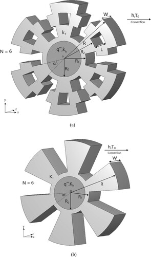
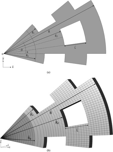
Figure 2. The (a) computational domain and (b) the grid system for the three-dimensional SSF with single IHS.

For the purpose of comparison with Feng et al. [20], all the notations used in this work will be the same as those reported by Feng et al. [20]. The three-dimensional dimensional heat conduction equations for the SSF and IHS are known as [20]: (1a) $\begin{array}{rl}& k_f\left(\frac{{\mathrm{\partial }}^{2}T}{\mathrm{\partial }{x}^2}+\frac{{\mathrm{\partial }}^{2}T}{\mathrm{\partial }{y}^2}+\frac{{\mathrm{\partial }}^{2}T}{\mathrm{\partial }{z}^2}\right)=0;\text{in SSF}\end{array}$(1a) (1b) $\begin{array}{rl}{k}_h& \left(\frac{{\mathrm{\partial }}^{2}T}{\mathrm{\partial }{x}^2}+\frac{{\mathrm{\partial }}^{2}T}{\mathrm{\partial }{y}^2}+\frac{{\mathrm{\partial }}^{2}T}{\mathrm{\partial }{z}^2}\right)+q^{\mathrm{\prime }\mathrm{\prime }\mathrm{\prime }}=0;\text{in IHS}\end{array}$(1b)

By defining the following dimensionless parameters (2a) $\begin{array}{rl}\tilde{T}& =\frac{T-T_{\mathrm{\infty }}}{q^{\mathrm{\prime }\mathrm{\prime }\mathrm{\prime }}{V}^{2/3}/k_f}\end{array}$(2a) (2b) $\begin{array}{rl}(\tilde{x},\tilde{y},\tilde{z},\tilde{R},{\tilde{R}}_0,{\tilde{R}}_1,{\tilde{R}}_2,\tilde{W})& =\frac{(x,y,z,R,R_0,R_1,R_2,W)}{V^{1/3}}\end{array}$(2b) where V = πR²W

If the volumes of SSF and IHS are provided, the following three constraints can be obtained: (3a) $\begin{array}{rl}1& =\pi {\tilde{R}}^2\tilde{W}\end{array}$(3a) (3b) $\begin{array}{rl}{\text{ϕ}}_0& =\frac{\pi {{\tilde{R}}_0}^2}{\pi {\tilde{R}}^2}\end{array}$(3b) (3c) $\begin{array}{rl}{\text{ϕ}}_1& =\frac{\frac{\pi ({\tilde{R}}^2-{{\tilde{R}}_1}^2)N\alpha }{2\pi }+\pi {{\tilde{R}}_1}^2}{\pi {\tilde{R}}^2}-{\text{ϕ}}_0\end{array}$(3c) where the volume fractions ${\text{ϕ}}_0=\frac{V_0}{V}$ and ${\text{ϕ}}_1=\frac{V_f}{V}$.

The non-dimensional energy and boundary condition equations for SSF and IHS can be obtained as [20]: (4a) $\begin{array}{rl}& \frac{{\mathrm{\partial }}^2\tilde{T}}{\mathrm{\partial }{\tilde{x}}^2}+\frac{{\mathrm{\partial }}^2\tilde{T}}{\mathrm{\partial }{\tilde{y}}^2}+\frac{{\mathrm{\partial }}^2\tilde{T}}{\mathrm{\partial }{\tilde{z}}^2}=0;\text{in SSF}\end{array}$(4a) (4b) $\begin{array}{rl}& -\frac{\mathrm{\partial }\tilde{T}}{\mathrm{\partial }\tilde{n}}=a\tilde{T};\text{on the surfaces of SSF}\end{array}$(4b) (5a) $\begin{array}{rl}& \frac{1}{\tilde{k}}\left(\frac{{\mathrm{\partial }}^2\tilde{T}}{\mathrm{\partial }{\tilde{x}}^2}+\frac{{\mathrm{\partial }}^2\tilde{T}}{\mathrm{\partial }{\tilde{y}}^2}+\frac{{\mathrm{\partial }}^2\tilde{T}}{\mathrm{\partial }{\tilde{z}}^2}\right)+1=0;\text{in IHS}\end{array}$(5a) (5b) $\begin{array}{rl}& -\frac{1}{\tilde{k}}\frac{\mathrm{\partial }\tilde{T}}{\mathrm{\partial }\tilde{n}}=a\tilde{T};\text{on the surfaces of IHS}\end{array}$(5b) where $\tilde{k}$=k_f/k_h and convective heat transfer coefficient $a=\frac{h{V}^{1/3}}{k_f}$.

Finally the dimensionless maximum thermal resistance (DMTR) with single IHS, ${\tilde{R}}_{t1}$, can be obtained as [20]: (6) ${\tilde{R}}_{t1}=\frac{{\tilde{T}}_{max}}{{\text{ϕ}}_0}$(6) Once the dimensionless temperature distribution is calculated, the maximum temperature ${\tilde{T}}_{max}$ can also be obtained and ${\tilde{R}}_{t1}$ can be computed from Equation (6).

Under the conditions that $\tilde{W}$, N, φ₀ and φ₁ are given, to satisfy three constraints in Equation (3), ${\tilde{R}}_1$ must be the design variable. Besides, Figure 2(a) shows the enlarged picture of one of the extended bodies, and the location of perforation can be identified if the variables ${\tilde{R}}_2\text{ and }\beta$ are known, i.e. ${\tilde{R}}_2\text{ and }\beta$ must be also the design variables. Therefore, the design variables for single IHS problem become $\{{\tilde{R}}_1,{\tilde{R}}_2,\beta \}$.

It can be learned from Figure 2(a) that when the splitting angle β approaches to zero, the SSF is identical to the HSF, which was examined by Feng et al. [20] previously. Due to the axial symmetry of the SSF with single IHS, for simplicity of calculations, the computational domain and the grid system for the three-dimensional SSF considered in this study is given in Figure 2(b).

The direct problem considered in the study is concerned with the determination of the domain temperature distributions when the geometry and thermal properties of SSF, IHS, and the boundary conditions are all given and known.

3. The snowflake-shaped fin design problem

For the present snowflake-shaped fin design problem with single IHS, the geometry of SSF Γ $(\tilde{x},\tilde{y},\tilde{z})=\mathrm{\Gamma }(\mathbf{\text{B}})$ is regarded as being unknown and it can be determined by the design variables ${\tilde{R}}_1,{\tilde{R}}_2\text{ and }\beta$ when the values of $\tilde{L}$, $\tilde{W}$, $\tilde{k}$, φ₀, φ₁, and N are given. Here the design variables B is regarded being unknown and $\mathbf{\text{B}}=\{B_i\}=\{B_1,B_2,B_3\}=\{{\tilde{R}}_1,{\tilde{R}}_2,\beta \}$, i indicates the index of design variables and i = 1–3. The lower and upper limits of the design variables are given as follows: $1.01{\tilde{R}}_0\le {\tilde{R}}_1\le 0.99{\tilde{R}}_2;1.01{\tilde{R}}_1\le {\tilde{R}}_2\le 0.99(\tilde{R}-\tilde{L});0<\beta \le \frac{\alpha }{2}$ Besides, to avoid overlapping of splitting parts of the extended bodies, the constraint $0<(2\beta +\alpha )\le \frac{2\pi }{N}$ is considered.

The present optimal fin design problem is expressed in the following statement: by utilizing the design variables B, design the optimal snowflake-shaped fin to minimize the maximum temperature of the fin domain under fixed fin volume condition. The cost function of this optimal fin design problem is expressed in the following form and need be minimized: (7) $J\text{[}\mathrm{\Gamma }(B_{\text{i}})\text{] }=[{\tilde{T}}_{max}(B_i){]}^2$(7) here ${\tilde{T}}_{max}$ represents the maximum domain temperature of fin.

Equation (7) is minimized with respect to the design variables Bi to obtain: (8) $\frac{\mathrm{\partial }J[\mathrm{\Gamma }(B_i)]}{\mathrm{\partial }{B}_i}=\left[\frac{\mathrm{\partial }{\tilde{T}}_{max}}{\mathrm{\partial }{B}_i}\right][{\tilde{T}}_{max}]=0$(8) where Equation (8) is linearized by expanding ${\tilde{T}}_{max}$ in Taylor series and keeping the first-order term. Thereafter a damping parameter μⁿ is added to the resultant expression for improving rate of convergence, finally the following iterative form of equation with Levenberg-Marquardt method [24] can be obtained as: (9) ${\mathbf{B}}^{\text{n + 1}}={\mathbf{B}}^{\text{n}}+\Delta \mathbf{B}$(9) where (10) $\text{(}\mathbf{F}\text{ + }{\mu }^{\text{n}}\mathrm{I}\text{)}\Delta \mathbf{B}=\mathbf{D}$(10) (11) $\mathbf{\text{F}}={\mathit{\vartheta }}^T\mathit{\vartheta }$(11) (12) $\mathbf{\text{D}}=\mathit{\vartheta }{T}_{{\tilde{T}}_{max}}$(12)

I is the identity matrix, and ϑ denotes the Jacobian matrix, defined as: (13) $\vartheta =\frac{\mathrm{\partial }{\tilde{T}}_{max}}{\mathrm{\partial }{\mathbf{B}}^{\text{T}}}$(13) the superscripts n and T indicate the iteration number and transpose matrix, respectively,

The Jacobian matrix ϑ is obtained by perturbing each unknown design variables B_i at one time and calculating the resultant change in maximum temperature of fin domain from the direct problem.

An iterative form for Equation (9) can be obtained as: (14) ${\mathbf{B}}^{\text{n + 1}}={\mathbf{B}}^{\text{n}}\text{ + (}{\vartheta }^{\text{T}}\vartheta \text{ + }{\mu }^{\text{n}}\mathbf{I}{\text{)}}^{-\text{1}}{\vartheta }^{\text{T}}{\tilde{T}}_{max}$(14) The Levenberg-Marquardt method is also called the damped least-squares (DLS) method and is used to solve non-linear least squares problems. The steepest-descent method is utilized in the beginning (i.e. ${\mu }^n\to \mathrm{\infty }$), then the value of μⁿ is decreased, and finally Newton's method is used (i.e. μⁿ = 0) to obtain the optimal solution. The choice of damping parameter μⁿ is reported in detail in Marquardt [24].

4. Computational procedure

The inverse design procedure for this snowflake-shaped fin design problem with LMM is now given below:

First, use the initial guess of design variables B⁰ to construct the initial shape of snowflake-shaped fin to begin the computation.

Step 1 Solve the direct problem to obtain the computed maximum domain temperature ${\tilde{T}}_{max}$.

Step 2 Calculate the Jacobian matrix ϑ from Equation (13).

Step 3 Calculate Bⁿ⁺¹ from Equation (14) and compute ${\tilde{T}}_{max}$.

Step 4 If the stopping criterion ε satisfy, stop the iterative process, otherwise, go to Step 1 and iterate.

5. Results and discussions

The objective of this study is to estimate the optimal geometry of snowflake-shaped fin by minimizing the maximum domain temperature ${\tilde{T}}_{max}$ under fixed fin volume condition. The optimal design examples for HSF provided by Feng et al. [20] will be considered as the benchmark problems in the present study, therefore the numerical results will be compared with those published by Feng et al. [20] to emphasize the superiority of using the present snowflake-shaped fin.

The grid-independent tests with the commercial code CFD-ACE+ code are performed based on the HSF, Figure 1(b), with the following conditions: $\tilde{W}=0.5$, $\tilde{k}=10$, φ₀ = 0.1, φ₁ = 0.5, R₁/R = 0.4 and N = 6. Due to the symmetric geometry of the HSF, the computational domain is considered to be only one-sixth of its physical domain.

Four different numerical structure grid numbers 9120; 20952; 29556; and 40760 are considered and the dimensionless maximum thermal resistance (DMTR) of HSF, ${\tilde{R}}_{t1,HSF}$, can be obtained as 1.9204, 1.9177, 1.9182 and 1.9188, respectively. The relative error for ${\tilde{R}}_{t1,HSF}$ between grid numbers 29556 and 40760 is 0.03%, which is small enough. Therefore, the grid number of order 30000 is chosen for all the computational cases in this work. The values of ${\tilde{R}}_{t1,HSF}$ computed by Feng et al. [20] with normal and refined mesh models are given as 1.9200 and 1.9215, respectively, and they are nearly identical to our values. Based on the above numerical verifications it can be concluded that the numerical solutions for HSF between the present and Feng et al. [20]’s studies are almost identical.

The stopping criterion for iterations of this study is defined as follows: (15) $\frac{|{{\tilde{T}}_{max}}^{n+1}\text{ - }{{\tilde{T}}_{max}}^n|}{{{\tilde{T}}_{max}}^n}\le \epsilon$(15) where the superscript n denotes iteration number and ε is chosen as 10⁻³ in this study.

Case 1 single IHS problems

For the purpose of comparison, the characteristic of minimum value of dimensionless maximum thermal resistance ${\tilde{R}}_{t1,\mathrm{m},\mathrm{HSF}}$ and (R₁/R)_opt,HSF versus $\tilde{W}$ (i.e. Figure 4 in [20]) for HSF is recalculated using LMM and CFD-ACE+ code with N = 6, $\tilde{L}=0\text{.17}$, $\tilde{k}=10$, φ₀ = 0.1 and φ₁ = 0.5 and are plotted in Figure 3.

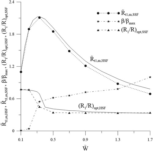
Figure 3. Variation of characteristic curves for HSF and SSF with single HIS versus $\tilde{W}$.

For the design problems of SSF with $\tilde{W}=0.5$, two different initial guesses of the design variables $\{{{\tilde{R}}^0}_1,{{\tilde{R}}^0}_2,{\beta }^0\}$ are used to examine the validity of this design algorithm, they are (i) {0.4 $\tilde{R}$, 0.44 $\tilde{R}$, 0.32^o} and (ii) {0.4 $\tilde{R}$, 0.44 $\tilde{R}$, α/3}, respectively. Here β = 0.32^o $\approx$ 0 represents the HSF. By using the LMM to minimize the cost function Equation (7)(3c) $\begin{array}{rl}{\text{ϕ}}_1& =\frac{\frac{\pi ({\tilde{R}}^2-{{\tilde{R}}_1}^2)N\alpha }{2\pi }+\pi {{\tilde{R}}_1}^2}{\pi {\tilde{R}}^2}-{\text{ϕ}}_0\end{array}$(3c) , the estimated design variables for initial guesses (i) and (ii) are obtained as {0.287, 0.290, 4.453} and {0.287, 0.290, 4.421}, respectively, and the corresponding minimum value of DMTR, ${\tilde{R}}_{t1,m,\text{S}SF}$, are both calculated as 1.856 and the value of ${\tilde{R}}_{t1,m,HFS}$ is obtained as 1.919. The estimated data is listed in Table 1.

Table 1. The initial and optimal design variables for SSF with single IHS.

	Initial guesses for SSF			Optimal variables for SSF			Optimal DMTR using SSF	Optimal DMTR using HSF	Reduction of DMTR
	${{\tilde{R}}^0}_1$	${{\tilde{R}}^0}_2$	${\beta }^0$(°)	${\tilde{R}}_1$	${\tilde{R}}_2$	$\beta$(°)	${\tilde{R}}_{t1,\mathrm{m},\mathrm{SSF}}$	${\tilde{R}}_{t1,\mathrm{m},\mathrm{HSF}}$	$\eta$(%)	Iterations
$\tilde{W}=0.5$	0.4$\tilde{R}$	0.44$\tilde{R}$	≈0 (0.32)	0.287	0.290	4.453	1.86	1.92	3.28	8
	0.4$\tilde{R}$	0.44$\tilde{R}$	$\frac{\alpha }{3}$	0.287	0.290	4.421	1.86		3.28	12
	0.4$\tilde{R}$	N/A	$\frac{\alpha }{3}$	0.273	N/A	5.992	1.85	1.92	3.54	12
$\tilde{W}=0.1$	0.37$\tilde{R}$	N/A	$\frac{\alpha }{3}$	1.380	N/A	0.081	1.10	1.10	0.18	3
$\tilde{W}=0.2$	0.37$\tilde{R}$	N/A	$\frac{\alpha }{3}$	0.970	N/A	0.396	1.90	1.90	0.32	4
$\tilde{W}=0.33$	0.37$\tilde{R}$	N/A	$\frac{\alpha }{3}$	0.441	N/A	5.351	2.11	2.13	0.80	3
$\tilde{W}=0.5$	0.37$\tilde{R}$	N/A	$\frac{\alpha }{3}$	0.273	N/A	6.067	1.85	1.92	3.54	17
$\tilde{W}=0.7$	0.37$\tilde{R}$	N/A	$\frac{\alpha }{3}$	0.228	N/A	6.461	1.49	1.57	5.53	8
$\tilde{W}=0.9$	0.37$\tilde{R}$	N/A	$\frac{\alpha }{3}$	0.200	N/A	7.061	1.21	1.31	7.13	8
$\tilde{W}=1.3$	0.37$\tilde{R}$	N/A	$\frac{\alpha }{3}$	0.165	N/A	7.647	0.88	0.97	9.48	5
$\tilde{W}=1.7$	0.37$\tilde{R}$	N/A	$\frac{\alpha }{3}$	0.147	N/A	9.813	0.69	0.78	11.55	8

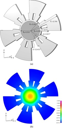
Since the estimations of the snowflake-shaped fin using both initial guesses are almost identical, only the results with initial guess (i) are plotted. The estimated shape of SSF and the temperature counter distribution are given in Figure 4(a,b), respectively. It can be seen from Table 1 that the estimated value of ${\tilde{R}}_2$ approaches to it lower bound, i.e. 1.01${\tilde{R}}_1$, for both initial guesses, it implies that the best location of the splitting point should be at ${\tilde{R}}_2={\tilde{R}}_1$.

Figure 4. The (a) optimal shape and (b) the temperature distribution of SSF with $\tilde{W}=0.5$ and single IHS.

To demonstrate the validation of the above observation, the design problem using design variables $\mathbf{\text{B}}=\{{\tilde{R}}_1,\beta \}$ is performed again and the initial guesses for the design variables $\{{{\tilde{R}}^0}_1,{\beta }^0\}$ are chosen as {0.4$\tilde{R}$, α/3}. The estimated results are listed in Table 1 and it can be learned that the estimated design variables are obtained as {0.273, 5.992}, and the corresponding ${\tilde{R}}_{t1,m,\text{SSF}}$ is calculated as 1.851. Indeed, it is better than the results using three design variables $\{{\tilde{R}}_1,{\tilde{R}}_2,\beta \}$, since the condition ${\tilde{R}}_2={\tilde{R}}_1$ is considered.

This finding can eliminate one design variable and makes $\{B_i\}=\{B_1,B_2\}=\{{\tilde{R}}_1,\beta \}$, i = 1–2, and speed up the computational time for the estimations. The condition ${\tilde{R}}_2={\tilde{R}}_1$ will be applied to all the remaining cases in this work.

Next, test cases with $\tilde{W}=0.1,0.2,0.33,0.5,0.7,0.9,1.3\text{ and }1.7$ are considered, different initial guesses of the design variables {${{\tilde{R}}^0}_1,{\beta }^0$} = {0.37$\tilde{R}$, α/3} will be assumed to test the validity of the design algorithm.

The initial guesses and estimated variables are listed in Table 1 and the estimated results are also plotted in Figure 3 versus$\tilde{W}$ for the values of ${\tilde{R}}_{t1,m,S\text{SF}}$, β/βmax and (R₁/R)_opt,SSF.

It can be learned that the estimated design variables using initial guesses $\{{{\tilde{R}}^0}_1,{\beta }^0\}=\{0.37\tilde{R},\alpha /3\}$ are obtained as {0.273, 6.067} for $\tilde{W}=0.5$, and the corresponding ${\tilde{R}}_{t1,m,\text{S}FS}$ is calculated as 1.851. The results are identical to those obtained by using initial guesses $\{{{\tilde{R}}^0}_1,{\beta }^0\}=\{0.4\tilde{R},a/3\}$, and this indicated again that different initial guess values will lead to the same optimal values. It is also noted from Figure 3 that the values of (R₁/R)_opt,SSF and (R₁/R)_opt,SSF are very close, except at $\tilde{W}$=0.33.

The value of β/βmax increases monotonously as $\tilde{W}$ increases. This implies that the splitting angle β becomes larger as the value of $\tilde{W}$ increases. It is because that when $\tilde{W}$ increases, the volume of sectorial extended bodies also increases and it is possible to provide more volume of the splitting parts of the fin to move outward.

The values of ${\tilde{R}}_{t1,m,\text{SSF}}$ are always smaller than those of ${\tilde{R}}_{t1,\mathrm{m},\mathrm{HSF}}$, the percentage reductions of ${\tilde{R}}_{t1,\mathrm{m},\mathrm{SSF}}$ with $\tilde{W}$ are varied from 0.182% to 11.553%, monotonously, when compared with the values of ${\tilde{R}}_{t1,m,HFS}$. The difference between ${\tilde{R}}_{t1,\mathrm{m},\mathrm{SSF}}$ and ${\tilde{R}}_{t1,\mathrm{m},\mathrm{HSF}}$ becomes larger and larger as $\tilde{W}$ increases and the number of iterations are always less than 17 for the cases examined here. It is thus demonstrated that the new design of SSF always has better heat dissipation performance than HSF under fix fin volume constraint, especially with larger $\tilde{W}$.

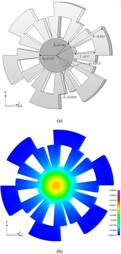
The estimated shape and temperature counter distribution of SSF with $\tilde{W}=0.2$ and $\tilde{W}=1.7$ are given in Figures 5 and 6, respectively. It can be learned from Figures 4–6 that when the value of $\tilde{W}$ decreases, the volume of sectorial extended bodies also decreases, and they are the location where the splitting take place. It is clear from Figure 5 that the volume of extended bodies is very small when $\tilde{W}$ is small, as a result, the extra fin surface due to splitting perforation is negligible and therefore the reduction of ${\tilde{R}}_{t1,\mathrm{m},\mathrm{SSF}}$ is also negligible.

Figure 5. The (a) optimal shape and (b) the temperature distribution of SSF with $\tilde{W}=0.2$ and single IHS.

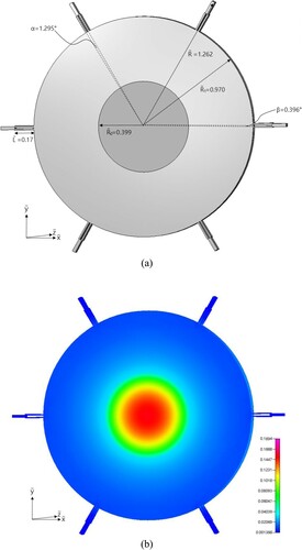
Figure 6. The (a) optimal shape and (b) the temperature distribution of SSF with $\tilde{W}=1.7$ and single IHS.

Case 2 two IHS problems (n=2)

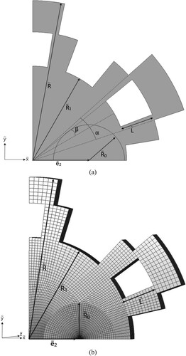
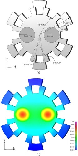
Figure 7(a,b) illustrate the shape and parameters of SSF and HSF, respectively, with six sectorial extended bodies (SEBs) and two IHSs, e₂ denotes the distance between the fin’s centre and IHS’s centre. Due to the axial symmetry of the SSF, only a quarter of the SSF is considered as the computational domain. Figure 8(a) indicates a quarter of SSF, the constraint equations can be satisfied and location of perforation can be identified if the variables ${\tilde{R}}_1\text{, }{\text{e}}_2\text{ and }\beta$ are known, i.e. the design variables for multiple IHS problems become $\{{\tilde{R}}_1\text{, }{\text{e}}_2\text{, }\beta \}$. The grid system for the three-dimensional SSF with two IHSs considered in case 2 is given in Figure 8(b).

Figure 7. The (a) snowflake-shaped and (b) helm-shaped fins with two IHSs.

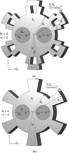
Figure 8. The (a) computational domain and (b) the grid system for the three-dimensional SSF with two IHSs.

The volume fractions φ₀ can be expressed as: (16) ${\text{ϕ}}_0=\frac{n\pi {{\tilde{R}}_0}^2}{\pi {\tilde{R}}^2}=\frac{V_0}{V}$(16) For HSF, when N,$\tilde{k}$, $\tilde{W}$, φ₀, φ₁ and n are given, ${\tilde{R}}_{tn,HSF}$ is function of the following two design variables, radius R₁ and the distance e_n, therefore for n = 2, ${\tilde{R}}_{t2,\mathrm{m},\mathrm{HSF}}$ can be obtained by the estimated optimal values of R₁ and e₂ using the present inverse design algorithm. For the purpose of numerical solution validations, the following two examples will be considered:

1. When N=6, a = 0.5, $\tilde{k}$=10,$\tilde{W}$=0.5, φ₀,=0.1, φ₁ = 0.5, n=2 and R₁/R=0.7 are considered for HSF, there is only one design variable e₂. By using the LMM, the optimal design variable can be obtained as e₂ = 0.325 and e₂/R = 0.407, as a result, ${\tilde{R}}_{t2,\mathrm{m},\mathrm{HSF}}$ is calculated as 1.262. From Figure 6 in [20], for the case with R1/R=0.7, the values of e₂/R and ${\tilde{R}}_{t2,\mathrm{m},\mathrm{HSF}}$ can be obtained approximately as 0.405 and 1.264, respectively. The values of e₂/R and ${\tilde{R}}_{t2,\mathrm{m},\mathrm{HSF}}$ calculated in this study and in [20] are almost identical.

2. When N=6, a = 0.5,$\tilde{k}$=10,$\tilde{W}$=0.5, φ₀,=0.1, φ₁ = 0.5 and n=2 are considered for HSF, now there are two design variables, R₁ and e₂. The optimal design variables are obtained as R₁ = 0.55 (R₁/R = 0.68) and e₂ = 0.317 (e₂/R = 0.397) using LMM, and ${\tilde{R}}_{t2,\mathrm{m},\mathrm{HSF}}$ is obtained as 1.261. Based on Figure 8 in [20], for the case with a = 0.5, the values of e₂/R, R₁/R and ${\tilde{R}}_{t2,\mathrm{m},\mathrm{HSF}}$ can be obtained approximately as 0.4, 0.68 and 1.262, respectively, again, those numbers are also almost identical. Based on the above two examples, the numerical solutions using the present solver and inverse design algorithm are thus validated.

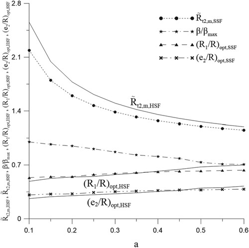
By using the following system variables for HSF: N=6, $\tilde{k}$=10,$\tilde{W}$=0.5, φ₀,=0.1, φ₁ = 0.5 and n=2, the characteristics of minimum value of dimensionless maximum thermal resistance ${\tilde{R}}_{t2,\mathrm{m},\mathrm{HSF}}$, (e₂/R)_opt,HSF and (R₁/R)_opt,HSF versus ‘a’, a = 0.1–0.6, (i.e. Figure 8 in [20]), with increment Δa = 0.05 are recalculated with LMM and CFD-ACE+ code and are plotted in Figure 9.

Figure 9. Variation of characteristic curves for HSF and SSF with two IHSs versus ‘a'.

The comparisons among the HSFs and SSFs will be analysed next. For n = 2, the design variables for SSH become {B_i} = {B₁, B₂, B₃} = {${\tilde{R}}_1,{\text{e}}_2\text{, }\beta$}, i = 1–3. The test cases with a = 0.1–0.6 with Δa = 0.05 are considered and the initial guesses of the design variables {${{\tilde{R}}^0}_1,{\text{ e}}_n^0,{\beta }^0$} = {0.63$\tilde{R}$, 0.38$\tilde{R}$, α/3} are assumed.

The initial guesses and estimated variables are summarized in Table 2 and the estimated results are also plotted in Figure 9 versus ‘a’ for the values of ${\tilde{R}}_{t2,\mathrm{m},\mathrm{SSF}}$, β/βmax, (e₂/R)_opt,SSF and (R₁/R)_opt,SSF. It is learned from Figure 9 that the values of (e₂/R)_opt and (R₁/R)_opt for SSF and HSF are very close and are increase monotonously when a increases, while the value of β/βmax decreases monotonously when a increases. It indicates that the angle of splitting becomes smaller as the value of ‘a’ increases.

Table 2. The initial and optimal design variables for SSF with two IHSs.

	Initial guesses for SSF			Optimal variables for SSF			Optimal DMTR using SSF	Optimal DMTR using HSF	Reduction of DMTR
	${{\tilde{R}}^0}_1$	$e_2^0$	${\beta }^0$(°)	${\tilde{R}}_1$	$e_2$	$\beta$(°)	${\tilde{R}}_{t2,\mathrm{m},\mathrm{SSF}}$	${\tilde{R}}_{t2,\mathrm{m},\mathrm{HSF}}$	$\eta$(%)	Iterations
$a=0.1$	0.63$\tilde{R}$	0.38$\tilde{R}$	$\frac{\alpha }{3}$	0.427	0.248	10.416	2.19	2.56	14.36	99
$a=0.15$	0.63$\tilde{R}$	0.38$\tilde{R}$	$\frac{\alpha }{3}$	0.437	0.257	10.085	1.80	2.04	11.94	41
$a=0.2$	0.63$\tilde{R}$	0.38$\tilde{R}$	$\frac{\alpha }{3}$	0.438	0.258	9.861	1.60	1.78	10.13	80
$a=0.25$	0.63$\tilde{R}$	0.38$\tilde{R}$	$\frac{\alpha }{3}$	0.458	0.273	9.478	1.47	1.62	8.85	91
$a=0.3$	0.63$\tilde{R}$	0.38$\tilde{R}$	$\frac{\alpha }{3}$	0.471	0.282	9.051	1.39	1.50	7.66	77
$a=0.35$	0.63$\tilde{R}$	0.38$\tilde{R}$	$\frac{\alpha }{3}$	0.480	0.288	8.646	1.32	1.42	6.77	30
$a=0.4$	0.63$\tilde{R}$	0.38$\tilde{R}$	$\frac{\alpha }{3}$	0.487	0.294	8.441	1.27	1.35	5.91	46
$a=0.45$	0.63$\tilde{R}$	0.38$\tilde{R}$	$\frac{\alpha }{3}$	0.494	0.299	8.181	1.24	1.30	5.22	39
$a=0.5$	0.63$\tilde{R}$	0.38$\tilde{R}$	$\frac{\alpha }{3}$	0.496	0.300	7.638	1.20	1.26	4.60	99
$a=0.55$	0.63$\tilde{R}$	0.38$\tilde{R}$	$\frac{\alpha }{3}$	0.501	0.304	7.417	1.18	1.23	4.16	42
$a=0.6$	0.63$\tilde{R}$	0.38$\tilde{R}$	$\frac{\alpha }{3}$	0.504	0.307	7.363	1.15	1.20	3.76	19

The values of ${\tilde{R}}_{t2,\mathrm{m},\mathrm{SSF}}$ are always smaller than the values of ${\tilde{R}}_{t2,\mathrm{m},\mathrm{HSF}}$, the percentage reductions of ${\tilde{R}}_{t2,\mathrm{m},\mathrm{SSF}}$ varied from 14.358% to 3.759% versus ‘a’ monotonously, when compared with the values of ${\tilde{R}}_{t2,\mathrm{m},\mathrm{HSF}}$, and the difference between ${\tilde{R}}_{t2,\mathrm{m},\mathrm{SSF}}$ and ${\tilde{R}}_{t2,\mathrm{m},\mathrm{HSF}}$becomes smaller and smaller as ‘a’ increases. The number of iterations are between 19 and 99 for the cases considered here. This shows that the SSF with two IHSs has better heat dissipation performance than HSF especially with smaller value of ‘a’. The estimated shape and temperature counter distribution of SSF with a = 0.3 are plotted in Figure 10(a,b), respectively.

Figure 10. The (a) optimal shape and (b) the temperature distribution of SSF with a = 0.3 and two IHSs.

Case 3 four IHS problems (n=4)

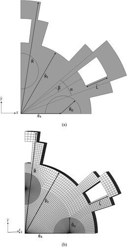
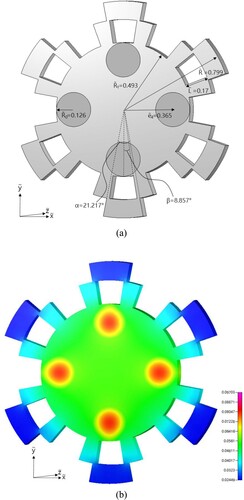
Figure 11(a,b) plot configurations of SSF and HSF, with N = 6 and n = 4, respectively, and e₄ indicates the distance from the fin’s centre to IHS’s centre. Again, only a quarter of the SSF is considered as the computational domain. Figure 12(a) plots a quarter of SSF, the design variables for four IHS problems become $\{{\tilde{R}}_1\text{, }{\text{e}}_4\text{, }\beta \}$. Figure 12(b) illustrates the grid system for the three-dimensional SSF with four IHSs considered in case 3.

Figure 11. The (a) snowflake-shaped and (b) helm-shaped fins with four IHSs.

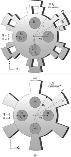
Figure 12. The (a) computational domain and (b) the grid system for the three-dimensional SSF with four IHSs.

Figure 13 plots the characteristics curves of ${\tilde{R}}_{t4,\mathrm{m},\mathrm{HSF}}$, (e₄/R)_opt,HSF and (R₁/R)_opt,HSF versus ‘a’ for HSF with N=6, $\tilde{k}$=10,$\tilde{W}$=0.5, φ₀,=0.1, φ₁ = 0.5 and n=4 (i.e. Figure 8 in [20]) using LMM and CFD-ACE+ code.

Figure 13. Variation of characteristic curves for HSF and SSF with four IHSs versus ‘a'.

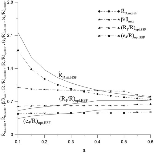
For n = 4, the design variables for SSF become {B_i} = {B₁, B₂, B₃} = {${\tilde{R}}_1,{\text{e}}_4\text{, }\beta$}, i = 1–3. The test cases with a = 0.1–0.6 with Δa = 0.05 are considered and the initial guesses of the design variables {$\{{{\tilde{R}}^0}_1,{\text{ e}}_n^0,{\beta }^0\}=\{0.63\tilde{R},0.38\tilde{R},\alpha /3\}$ are also assumed. The design processes are performed again and the estimated variables are listed in Table 3 and are also plotted in Figure 13 versus ‘a’ for the values of ${\tilde{R}}_{t4,\mathrm{m},\mathrm{SSF}}$, β/βmax, (e₄/R)_opt,SSF and (R₁/R)_opt,SSF. It is clear from Figure 13 that when ‘a’ is increased, the value of β/βmax decreases monotonously and the values of ${\tilde{R}}_{t4,\mathrm{m},\mathrm{SSF}}$ are also smaller than the values of ${\tilde{R}}_{t4,\mathrm{m},\mathrm{HSF}}$. Besides, it is also noticed that the boundary of IHS regions approach to ${\tilde{R}}_1$ for the cases with n = 4, as a result, if it requires a shorter computational time, the constraint e₄+R₀ = R₁ can be utilized and the design variable e₄ can be eliminated.

Table 3. The initial and optimal design variables for SSF with four IHSs.

	Initial guesses for SSF			Optimal variables for SSF			Optimal DMTR using SSF	Optimal DMTR using HSF	Reduction of DMTR
	${{\tilde{R}}^0}_1$	$e_4^0$	${\beta }^0$(°)	${\tilde{R}}_1$	$e_4$	$\beta$(°)	${\tilde{R}}_{t4,\mathrm{m},\mathrm{SSF}}$	${\tilde{R}}_{t4,\mathrm{m},\mathrm{HSF}}$	$\eta$(%)	Iterations
$a=0.1$	0.63$\tilde{R}$	0.38$\tilde{R}$	$\frac{\alpha }{3}$	0.480	0.353	9.414	1.78	2.16	17.63	23
$a=0.15$	0.63$\tilde{R}$	0.38$\tilde{R}$	$\frac{\alpha }{3}$	0.488	0.361	9.090	1.38	1.64	15.72	11
$a=0.2$	0.63$\tilde{R}$	0.38$\tilde{R}$	$\frac{\alpha }{3}$	0.491	0.364	8.987	1.18	1.37	14.00	8
$a=0.25$	0.63$\tilde{R}$	0.38$\tilde{R}$	$\frac{\alpha }{3}$	0.493	0.365	8.890	1.05	1.20	12.46	24
$a=0.3$	0.63$\tilde{R}$	0.38$\tilde{R}$	$\frac{\alpha }{3}$	0.493	0.365	8.857	0.97	1.09	11.18	19
$a=0.35$	0.63$\tilde{R}$	0.38$\tilde{R}$	$\frac{\alpha }{3}$	0.493	0.366	8.807	0.91	1.01	10.20	34
$a=0.4$	0.63$\tilde{R}$	0.38$\tilde{R}$	$\frac{\alpha }{3}$	0.493	0.366	8.768	0.86	0.94	8.61	35
$a=0.45$	0.63$\tilde{R}$	0.38$\tilde{R}$	$\frac{\alpha }{3}$	0.494	0.366	8.701	0.82	0.89	7.42	49
$a=0.5$	0.63$\tilde{R}$	0.38$\tilde{R}$	$\frac{\alpha }{3}$	0.494	0.366	8.655	0.79	0.85	6.71	90
$a=0.55$	0.63$\tilde{R}$	0.38$\tilde{R}$	$\frac{\alpha }{3}$	0.512	0.378	7.908	0.77	0.82	5.89	55
$a=0.6$	0.63$\tilde{R}$	0.38$\tilde{R}$	$\frac{\alpha }{3}$	0.520	0.384	7.569	0.75	0.79	5.34	53

The percentage reductions of ${\tilde{R}}_{t4,\mathrm{m},\mathrm{SSF}}$ vary from 17.631% to 5.337% monotonously as the convective heat transfer parameter ‘a’ is increased from 0.1–0.6, when compared with the values of ${\tilde{R}}_{t4,\mathrm{m},\mathrm{HSF}}$. The difference between ${\tilde{R}}_{t4,\mathrm{m},\mathrm{SSF}}$ and ${\tilde{R}}_{t4,\mathrm{m},\mathrm{HSF}}$ also becomes smaller and smaller as ‘a’ increases. Figure 14(a,b) illustrate the estimated snowflake-shaped fins and temperature distribution with a = 0.3, respectively.

Figure 14. The (a) optimal shape and (b) the temperature distribution of SSF with a = 0.3 and four IHSs.

Based on the above numerical examples it can be concluded that the optimal SSF can be obtained successfully with LMM algorithm under fixed fin volume constraint and indeed the heat dissipation capacity can be improved when compared with the original design of HSF.

6. Conclusions

A three-dimensional inverse shape design problem in determining the optimal geometry of snowflake-shaped fins (SSF) based on the minimization of the maximum domain temperature of fin is examined successfully in this work with different number of internal heat sources. The dimensionless maximum thermal resistance (DMTR) of the estimated SSF are then compared with those obtained by HSF [20], under the same design conditions. Based on the estimated results the following conclusions can be drawn: (i) For the case of single IHS, the heat dissipation performance of the present snowflake-shaped fins is always better than that of the helm-shaped fins especially with larger$\tilde{W}$. The volume of extended bodies becomes smaller and smaller as $\tilde{W}$ decreases, therefore the reduction of ${\tilde{R}}_{t1,\mathrm{m},\mathrm{SSF}}$ is also negligible when$\tilde{W}$is less than 0.33. (ii) For the case of multiple IHSs with n = 2 and 4, the resultant DMTRs for SSF are always lower than those of HSF, the reduction of DMTR is significant as the convective heat transfer coefficient becomes small, when a = 0.1, the reduction can be as large as 14.358% and 17.631% for n = 2 and 4, respectively.

Disclosure statement

No potential conflict of interest was reported by the authors.

Additional information

Funding

This work was supported in part through the Ministry of Science and Technology, Taiwan [Grant number, MOST-108-2221-E-006-088-MY3].

References

- Huang CH, Hsiao JH. An inverse design problem in determining the optimum shape of spine and longitudinal fins. Numeri Heat Transf A. 2007;43:155–177. doi: 10.1080/10407780307326
- Aziz A, Bouaziz MN. A least squares method for a longitudinal fin with temperature dependent internal heat generation and thermal conductivity. Energy Convers Manage. 2011;52:2876–2882. doi: 10.1016/j.enconman.2011.04.003
- Lindstedt M, Lampio K, Karvinen R. Optimal shapes of straight fins and finned heat sinks, Trans. ASME. J. Heat Transf. 2015;137:061006. doi: 10.1115/1.4029854
- Huang CH, Wu HH. A Fin design problem in determining the optimum shape of Non-Fourier spine and longitudinal fins. CMC, Comput Mater Contin. 2007;5:197–211.
- Bejan A, Almogbel M. Constructal T-shaped fin. Int J Heat Mass Transf. 2000;43:2101–2115. doi: 10.1016/S0017-9310(99)00283-5
- Lorenzini G, Moretti S. A CFD application to optimize T-shaped fins: comparisons to the constructal theory’s results. ASME Trans. J Electron Packaging. 2007;129:324–327. doi: 10.1115/1.2756852
- Bhanja D, Kundu B. Radiation effect on optimum design analysis of a constructal T-shaped fin with variable thermal conductivity. Heat Mass Transf. 2012;48:109–122. doi: 10.1007/s00231-011-0845-1
- Lorenzini G, Medici M, Rocha LAO. Convective analysis of constructal Tshaped fins. J Eng Thermophys. 2014;23:98–104. doi: 10.1134/S1810232814020027
- Hazarika SA, Bhanja D, Nath S, et al. Analytical solution to predict performance and optimum design parameters of a constructal T-shaped fin with simultaneous heat and mass transfer. Energy. 2015;84:303–316. doi: 10.1016/j.energy.2015.02.102
- Lorenzini G, Moretti S. Numerical analysis on heat removal from Y-shaped fins: efficiency and volume occupied for a new approach to performance optimization. Int J Therm Sci. 2007;46:573–579. doi: 10.1016/j.ijthermalsci.2006.08.004
- Xie ZH, Chen LG, Sun FR. Constructal optimization of twice level Y-shaped assemblies of fins by taking maximum thermal resistance minimization as objective. Sci China Technol Sci. 2010;53:2756–2764. doi: 10.1007/s11431-010-4037-x
- Hajmohammadi MR, Poozesh S, Hosseini R. Radiation effect on constructal design analysis of a T-Y-shaped assembly of fins. J Therm Sci Technol. 2012;7:677–692. doi: 10.1299/jtst.7.677
- Lorenzini G, Rocha LAO. Constructal design of T-Y assembly of fins for an optimized heat removal. Int J Heat Mass Transf. 2009;52:1458–1463. doi: 10.1016/j.ijheatmasstransfer.2008.09.007
- Almogbel M, Bejan A. Cylindrical of pin fins. Int J Heat Mass Transf. 2000;43:4285–4297. doi: 10.1016/S0017-9310(00)00049-1
- Bello-Ochende T, Meyer JP, Bejan A. Constructal multi-scale pin-fins. Int J Heat Mass Transf. 2010;53:2773–2779. doi: 10.1016/j.ijheatmasstransfer.2010.02.021
- Hajmohammadi MR, Poozesh S, Nourazar SS, et al. Optimal architecture of heat generating pieces in a fin. J Mech Sci Technol. 2013;27:1143–1149. doi: 10.1007/s12206-013-0217-5
- Gong SW, Chen LG, Feng HJ, et al. Constructal optimization of cylindrical heat sources surrounded with a fin based on minimization of hot spot temperature. Int Commun Heat Mass Transf. 2015;68:1–7. doi: 10.1016/j.icheatmasstransfer.2015.08.004
- Kundu B, Lee KS, Campo A. An ease of analysis for optimum design of an annular step fin. Int J Heat Mass Transf. 2015;85:221–227. doi: 10.1016/j.ijheatmasstransfer.2015.01.111
- Huang CH, Chung YL. An inverse problem in determining the optimum shapes for partially wet annular fins based on efficiency maximization. Int J Heat Mass Transf. 2015;90:364–375. doi: 10.1016/j.ijheatmasstransfer.2015.06.070
- Feng H, Chen L, Xie Z, et al. Constructal design for helm-shaped fin with internal heat sources. Int J Heat Mass Transf. 2017;110:1–6. doi: 10.1016/j.ijheatmasstransfer.2017.02.074
- Chin SB, Foo JJ, Lai YL, et al. Forced convective heat transfer enhancement with perforated pin fins. Heat Mass Transf. 2013;49:1447–1458. doi: 10.1007/s00231-013-1186-z
- Huang CH, Liu YC, Ay H. The design of optimum perforation diameters for Pin Fin array for heat transfer Enhancement. Int J Heat Mass Transf. 2015;84:752–765. doi: 10.1016/j.ijheatmasstransfer.2014.12.065
- Huang CH, Chen MH. An Estimation of the optimum shape and perforation diameters for Pin Fin Arrays. Int J Heat Mass Transf. 2019;131:72–84. 2019. doi: 10.1016/j.ijheatmasstransfer.2018.11.019
- Marquardt DM. An algorithm for least-squares estimation of nonlinear parameters. J Soc Indust Appl Math. 1963;11:431–441. doi: 10.1137/0111030
- Huang CH, Wu HH. An inverse Hyperbolic heat conduction problem in Estimating surface heat Flux by Conjugate Gradient method. J Phys D: Appl Phys. 2006;39:4087–4096. doi: 10.1088/0022-3727/39/18/020
- CFD-ACE+ user’s manual. ESI-CFD Inc. 2005.