Identification of the timewise thermal conductivity in a 2D heat equation from local heat flux conditions

ABSTRACT

The aim of this paper is to identify numerically the timewise thermal conductivity coefficients in the two-dimensional heat equation in a rectangular domain using initial and Dirichlet boundary conditions and the local heat flux as over-specification conditions. The measurement data represented by the local heat flux is shown to ensure the unique solvability of the inverse problem solution. The two-dimensional inverse problem is discretized using an alternating direction explicit method. The resulting constrained optimization problem is minimized iteratively by employing the MATLAB subroutine. Exact and noisy input data are inverted numerically. The  root mean square error values for various noise levels p for both smooth and non-smooth continuous timewise thermal conductivity coefficients Examples are compared. Numerical results are presented and discussed in order to illustrate the performance of the inversion for thermal conductivity components identification. This study will be significant to researchers working on computational and mathematical methods for solving inverse coefficient identification problems with applications in heat transfer and porous media.

Keywords:

• Inverse problem
• two-dimensional heat equation
• thermal conductivity
• local heat flux conditions
• nonlinear optimization

2010 Mathematics Subject Classifications:

• 65-XX
• 65Mxx
• 35R35

1. Introduction

The identification problems of the thermal conductivity/diffusivity coefficients in the parabolic partial differential equation from the local heat flux and/or non-local boundary measurements have received important attention from many researchers in the past, see [1–6] to mention only a few. The reconstruction of thermal conductivity coefficient along with the temperature in the heat equation from the non-local linear combination of heat flux and with local heat flux measurements has been investigated in [7] and [8], respectively. The determination of the orthotropic thermal conductivity coefficients and the temperature in the two-dimensional parabolic heat equation from the non-local heat flux over-specification conditions has been investigated in [9].

In recent years, the inverse heat conduction problems have received widespread attention in engineering applications [10,11]. Mera et al. [12] estimated the unknown conductivity coefficients and the unknown boundary data for the two-dimensional heat conduction problem in an anisotropic medium. Reddy and Dulikravich [13] determined simultaneously the spatially varying thermal conductivity and specific heat using boundary temperature measurements. Reddy et al. [14] estimated a single spatially varying material property (thermal conductivity) based on the solutions of a steady-state version of the heat conduction equation.

In a recent paper, [15], the authors have investigated the recovery of the time-dependent thermal conductivity coefficients $a_1(t)$ and $a_2(t)$ of an orthotropic rectangular conductor along with the temperature $u(x,y,t)$ in a two-dimensional problem given by the parabolic heat equation $u_t=a_1(t)u_{xx}+a_2(t)u_{yy}+f(x,y,t),$ from non-local over-specification conditions $a_1(t)({\nu }_{11}(t)u_x(0,y_0,t)+{\nu }_{12}(t)u_x(h,y_0,t))={\varkappa }_1(t),$ and $a_2(t)({\nu }_{21}(t)u_y(x_0,0,t)+{\nu }_{22}(t)u_y(x_0,l,t))={\varkappa }_2(t),$ where $x_0$, $y_0$ are fixed values from the intervals $(0,h)$ and $(0,l)$, and h, l are given positive quantities. When ${\nu }_{11}={\nu }_{21}=1$ and ${\nu }_{21}={\nu }_{22}=0$, the above non-local over-specification conditions become (5(5) $\begin{array}{rl}& a_1(t)\frac{\mathrm{\partial }u}{\mathrm{\partial }x}(0,Y_0,t)={\nu }_1(t),t\in [0,T],\end{array}$(5) ) and (6(6) $\begin{array}{rl}& a_2(t)\frac{\mathrm{\partial }u}{\mathrm{\partial }y}(X_0,0,t)={\nu }_2(t),t\in [0,T],\end{array}$(6) ), respectively. In this paper, we generalize the above non-local over-specifications to the local heat flux measurements (5(5) $\begin{array}{rl}& a_1(t)\frac{\mathrm{\partial }u}{\mathrm{\partial }x}(0,Y_0,t)={\nu }_1(t),t\in [0,T],\end{array}$(5) ) and (6(6) $\begin{array}{rl}& a_2(t)\frac{\mathrm{\partial }u}{\mathrm{\partial }y}(X_0,0,t)={\nu }_2(t),t\in [0,T],\end{array}$(6) ) for a more general two-dimensional parabolic heat equation, as described in the next section. The inverse problem investigated in this paper has already been proved to be locally uniquely solvable, but no numerical identification has been attempted so far, and it is the aim of the current research to undertake the numerical solution of this problem. In this work, the novelty consists in the development of a numerical optimization method for solving this nonlinear inverse coefficient problem for the two-dimensional heat equation. Numerically, the implementation is realized using the MATLAB subroutine lsqnonlin.

The structure of the paper is as follows. The mathematical formulation of the two-dimensional heat equation is formulated in Section 2. The numerical solution of the direct problem based on an alternating direction explicit method is presented in Section 3. The numerical solution of the inverse problem based on the minimization of the nonlinear least-squares objective function is introduced in Section 4. Numerical results are presented and discussed in Section 5. Finally, conclusions are given in Section 6.

2. Statement of the 2D heat equation problem

We consider an inverse problem of identifing the timewise thermal conductivity coefficients $a_1(t)>0$ and $a_2(t)>0$ in the two-dimensional heat equation [16], (1) $\begin{array}{rl}\frac{\mathrm{\partial }u}{\mathrm{\partial }t}(x,y,t)& =a_1(t)b_1(x)\frac{{\mathrm{\partial }}^{2}u}{\mathrm{\partial }{x}^2}(x,y,t)+a_2(t)b_2(y)\frac{{\mathrm{\partial }}^{2}u}{\mathrm{\partial }{y}^2}(x,y,t)+c_1(x,y,t)\frac{\mathrm{\partial }u}{\mathrm{\partial }x}(x,y,t)\\ & +c_2(x,y,t)\frac{\mathrm{\partial }u}{\mathrm{\partial }y}(x,y,t)+c_3(x,y,t)u(x,y,t)+f(x,y,t),(x,y,t)\in Q_T,\end{array}$(1) where $b_1>0$, $b_2>0$ are known space variations, $c_1$, $c_2$ are known velocity representing convective flow, $c_3$ is a known absorption coefficient, f is a known heat source, u is a unknown temperature in the rectangular domain $Q_T=\{(x,y,t):0<x<h,0<y<l,0<t<T\}$, subject to the initial condition (2) $u(x,y,0)=\phi (x,y),(x,y)\in [0,h]\times [0,l],$(2) the Dirichlet boundary conditions (3) $\begin{array}{rl}u(0,y,t)& ={\mu }_1(y,t),u(h,y,t)={\mu }_2(y,t),(y,t)\in [0,l]\times [0,T],\end{array}$(3) (4) $\begin{array}{rl}u(x,0,t)& ={\mu }_3(x,t),u(x,l,t)={\mu }_4(x,t),(x,t)\in [0,h]\times [0,T],\end{array}$(4) and the local heat flux over-specification conditions (5) $\begin{array}{rl}& a_1(t)\frac{\mathrm{\partial }u}{\mathrm{\partial }x}(0,Y_0,t)={\nu }_1(t),t\in [0,T],\end{array}$(5) (6) $\begin{array}{rl}& a_2(t)\frac{\mathrm{\partial }u}{\mathrm{\partial }y}(X_0,0,t)={\nu }_2(t),t\in [0,T],\end{array}$(6) where $X_0$, $Y_0$ are fixed values from the intervals $(0,h)$ and $(0,l)$, where h, l are given positive numbers, and $\phi (x,y)$, ${\mu }_1(y,t),{\mu }_2(y,t),{\mu }_3(x,t),{\mu }_4(x,t)$ 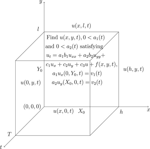are given functions satisfying compatibility conditions. The geometry of the inverse problem under investigation is shown in Figure 1.

Figure 1. Geometry of the inverse problem under investigation.

The local existence and uniqueness of solution of the inverse problem (1(1) $\begin{array}{rl}\frac{\mathrm{\partial }u}{\mathrm{\partial }t}(x,y,t)& =a_1(t)b_1(x)\frac{{\mathrm{\partial }}^{2}u}{\mathrm{\partial }{x}^2}(x,y,t)+a_2(t)b_2(y)\frac{{\mathrm{\partial }}^{2}u}{\mathrm{\partial }{y}^2}(x,y,t)+c_1(x,y,t)\frac{\mathrm{\partial }u}{\mathrm{\partial }x}(x,y,t)\\ & +c_2(x,y,t)\frac{\mathrm{\partial }u}{\mathrm{\partial }y}(x,y,t)+c_3(x,y,t)u(x,y,t)+f(x,y,t),(x,y,t)\in Q_T,\end{array}$(1) )–(6(6) $\begin{array}{rl}& a_2(t)\frac{\mathrm{\partial }u}{\mathrm{\partial }y}(X_0,0,t)={\nu }_2(t),t\in [0,T],\end{array}$(6) ) were established in [16] and read as stated in the following two theorems.

Theorem 2.1

Suppose that the following assumptions are satisfied:

(A1)	$\begin{array}{rl}& \phi (x,y)\in C^2(\overline{D}),\mathrm{where}D:=\{(x,y):0<x<h,0<y<l\},\\ & {\mu }_i(y,t)\in C^{2,1}([0,l]\times (0,T]),i=1,2,{\mu }_i(x,t)\in C^{2,1}([0,h]\times (0,T]),\\ & i=3,4,{\nu }_i(t)\in C[0,T],i=1,2,f(x,y,t)\in C^{1,1,0}(\overline{Q_T}),b_1(x)\in C^1[0,h],\\ & b_2(y)\in C^1[0,l],c_i(x,y,t)\in C^{1,1,0}(\overline{Q_T}),i=1,2,3;\end{array}$
(A2)	$\begin{array}{rl}& \phi (x,y)\ge 0,{\phi }_x(x,y)>0,{\phi }_y(x,y)>0,(x,y)\in \overline{D},{\mu }_1(y,t)\ge 0,{\mu }_2(y,t)\ge 0,\\ & {\mu }_{1_y}(y,t)>0,{\mu }_{2_y}(y,t)>0,{\mu }_{1_{yy}}(y,t)\ge 0,{\mu }_{2_{yy}}(y,t)\ge 0,(y,t)\in [0,l]\times [0,T],\\ & {\mu }_3(t)\ge 0,{\mu }_4(t)\ge 0,{\mu }_{3_x}(t)>0,{\mu }_{4_x}(t)>0,{\mu }_{3_{xx}}(x,t)\ge 0,{\mu }_{4_{xx}}(x,t)\ge 0,\\ & (x,t)\in [0,h]\times [0,T],f(x,y,t)\ge 0,f_x(x,y,t)>0,f_y(x,y,t)>0,c_1(0,y,t)<0,\\ & c_1(h,y,t)>0,c_2(x,0,t)<0,c_2(x,l,t)>0,c_{1_y}(x,y,t)\ge 0,c_{2_x}(x,y,t)\ge 0,\\ & c_{3_x}(x,y,t)\ge 0,c_{3_y}(x,y,t)\ge 0,(x,y,t)\in (\overline{Q_T}),b_1(x)>0,x\in [0,h],\\ & b_2(y)>0,y\in [0,l],{\nu }_i(t)\ne 0,i=1,2,t\in [0,T];\end{array}$
(A3)	$\begin{array}{rl}& {\mu }_{1_t}(y,t)-c_2(0,y,t){\mu }_{1_y}(y,t)-c_3(0,y,t){\mu }_1(y,t)-f(0,y,t)<0,\\ & {\mu }_{2_t}(y,t)-c_2(h,y,t){\mu }_{2_y}(y,t)-c_3(h,y,t){\mu }_2(y,t)-f(h,y,t)>0,\\ & {\mu }_{3_t}(x,t)-c_1(x,0,t){\mu }_{3_x}(x,t)-c_3(x,0,t){\mu }_3(x,t)-f(x,0,t)<0,\\ & {\mu }_{4_t}(x,t)-c_1(x,l,t){\mu }_{4_x}(x,t)-c_3(x,l,t){\mu }_4(x,t)-f(x,l,t)>0;\end{array}$
(A4)	$\begin{array}{rl}{\mu }_1(y,0)& =\phi (0,y),{\mu }_2(y,0)=\phi (h,y),{\mu }_3(x,0)=\phi (x,0),{\mu }_4(x,0)=\phi (x,l),\\ {\mu }_1(0,t)& ={\mu }_3(0,t),{\mu }_1(l,t)={\mu }_4(0,t),{\mu }_2(0,t)={\mu }_3(h,t),{\mu }_2(l,t)={\mu }_4(h,t).\end{array}$

Then, there exists $T_0\in (0,T],$ which is determined by the input data, such that the problem (1(1) $\begin{array}{rl}\frac{\mathrm{\partial }u}{\mathrm{\partial }t}(x,y,t)& =a_1(t)b_1(x)\frac{{\mathrm{\partial }}^{2}u}{\mathrm{\partial }{x}^2}(x,y,t)+a_2(t)b_2(y)\frac{{\mathrm{\partial }}^{2}u}{\mathrm{\partial }{y}^2}(x,y,t)+c_1(x,y,t)\frac{\mathrm{\partial }u}{\mathrm{\partial }x}(x,y,t)\\ & +c_2(x,y,t)\frac{\mathrm{\partial }u}{\mathrm{\partial }y}(x,y,t)+c_3(x,y,t)u(x,y,t)+f(x,y,t),(x,y,t)\in Q_T,\end{array}$(1) )–(6(6) $\begin{array}{rl}& a_2(t)\frac{\mathrm{\partial }u}{\mathrm{\partial }y}(X_0,0,t)={\nu }_2(t),t\in [0,T],\end{array}$(6) ) has a solution $(a_1(t),a_2(t),u(x,y,t))\in C^1[0,T_0]\times C^1[0,T_0]\times C^{2,1}(\overline{Q_{T_0}}),$ with $a_i(t)>0$ for $t\in [0,T_0],$ i = 1, 2.

Theorem 2.2

Suppose that the condition ${\nu }_i(t)>0,$ i = 1,2 for $t\in [0,T]$ is satisfied. Then, the inverse problem (1(1) $\begin{array}{rl}\frac{\mathrm{\partial }u}{\mathrm{\partial }t}(x,y,t)& =a_1(t)b_1(x)\frac{{\mathrm{\partial }}^{2}u}{\mathrm{\partial }{x}^2}(x,y,t)+a_2(t)b_2(y)\frac{{\mathrm{\partial }}^{2}u}{\mathrm{\partial }{y}^2}(x,y,t)+c_1(x,y,t)\frac{\mathrm{\partial }u}{\mathrm{\partial }x}(x,y,t)\\ & +c_2(x,y,t)\frac{\mathrm{\partial }u}{\mathrm{\partial }y}(x,y,t)+c_3(x,y,t)u(x,y,t)+f(x,y,t),(x,y,t)\in Q_T,\end{array}$(1) )–(6(6) $\begin{array}{rl}& a_2(t)\frac{\mathrm{\partial }u}{\mathrm{\partial }y}(X_0,0,t)={\nu }_2(t),t\in [0,T],\end{array}$(6) ) cannot have more than one solution in the class $(a_1(t),a_2(t),u(x,y,t))\in C^1[0,T]\times C^1[0,T]\times C^{2,1}(\overline{Q_T}),$ with $a_i(t)>0$ for $t\in [0,T],$ i = 1, 2.

3. Numerical solution of direct problem

In this section, we consider the direct initial boundary value problem (1(1) $\begin{array}{rl}\frac{\mathrm{\partial }u}{\mathrm{\partial }t}(x,y,t)& =a_1(t)b_1(x)\frac{{\mathrm{\partial }}^{2}u}{\mathrm{\partial }{x}^2}(x,y,t)+a_2(t)b_2(y)\frac{{\mathrm{\partial }}^{2}u}{\mathrm{\partial }{y}^2}(x,y,t)+c_1(x,y,t)\frac{\mathrm{\partial }u}{\mathrm{\partial }x}(x,y,t)\\ & +c_2(x,y,t)\frac{\mathrm{\partial }u}{\mathrm{\partial }y}(x,y,t)+c_3(x,y,t)u(x,y,t)+f(x,y,t),(x,y,t)\in Q_T,\end{array}$(1) )–(4(4) $\begin{array}{rl}u(x,0,t)& ={\mu }_3(x,t),u(x,l,t)={\mu }_4(x,t),(x,t)\in [0,h]\times [0,T],\end{array}$(4) ), where $a_1(t),$ $a_2(t),$ $b_1(x)$, $b_2(y)$, $c_i(x,y,t)$, $i=\overline{1,3}$, $f(x,y,t),$ $\phi (x,y),$ ${\mu }_i(y,t),$ i = 1, 2, and ${\mu }_i(x,t),$ i = 3, 4 are known and the solution $u(x,y,t)$ is to be determined together with the quantities of interest ${\nu }_i(t),$ $i=1,2$. We subdivide the solution domain $Q_T$ into $M_1$, $M_2$ and N subintervals of equal step lengths $\mathrm{\Delta }x,$ $\mathrm{\Delta }y$ and $\mathrm{\Delta }t,$ where $\mathrm{\Delta }x=h/M_1,$ $\mathrm{\Delta }y=l/M_2,$ and $\mathrm{\Delta }t=T/N,$ respectively. At the node $(i,j,n),$ we denote $u_{i,j}^n:=u(x_i,y_j,t_n),$ where $x_i=i\mathrm{\Delta }x,$ $y_j=j\mathrm{\Delta }y,$ $t_n=n\mathrm{\Delta }t$, $a_1^n:=a_1(t_n)$, $a_2^n:=a_2(t_n)$, $c_{1_{i,j}}^n:=c_1(x_i,y_j,t_n)$, $c_{2_{i,j}}^n:=c_2(x_i,y_j,t_n)$, $c_{3_{i,j}}^n:=c_3(x_i,y_j,t_n)$, $b_{1_i}:=b_1(x_i)$, $b_{2_j}:=b_2(y_j)$ and $f_{i,j}^n:=f(x_i,y_j,t_n)$ for $i=\overline{0,M_1},$ $j=\overline{0,M_2}$, $n=\overline{0,N}$.

Alternating direction explicit (ADE) method makes use of two approximations that are implemented for computations proceeding in alternating directions, e.g. from left to right and from right to left, with each approximation being explicit in its respective direction of computation [17–19]. The most important advantage of numerical simulation is the low cost and high computational speed. Furthermore, the numerical scheme possesses the advantage of the implicit methods, i.e. no severe limitation in the size of the time increment. Also, the ADE has another advantage, namely, that is unconditionally stable. For solving the direct problem (1(1) $\begin{array}{rl}\frac{\mathrm{\partial }u}{\mathrm{\partial }t}(x,y,t)& =a_1(t)b_1(x)\frac{{\mathrm{\partial }}^{2}u}{\mathrm{\partial }{x}^2}(x,y,t)+a_2(t)b_2(y)\frac{{\mathrm{\partial }}^{2}u}{\mathrm{\partial }{y}^2}(x,y,t)+c_1(x,y,t)\frac{\mathrm{\partial }u}{\mathrm{\partial }x}(x,y,t)\\ & +c_2(x,y,t)\frac{\mathrm{\partial }u}{\mathrm{\partial }y}(x,y,t)+c_3(x,y,t)u(x,y,t)+f(x,y,t),(x,y,t)\in Q_T,\end{array}$(1) )–(4(4) $\begin{array}{rl}u(x,0,t)& ={\mu }_3(x,t),u(x,l,t)={\mu }_4(x,t),(x,t)\in [0,h]\times [0,T],\end{array}$(4) ) the ADE is as follows.

Let ${\tilde{u}}_{i,j}^n$ and ${\tilde{v}}_{i,j}^n$ be the solutions of the following equations which are multilevel finite difference discretization of Equation (1(1) $\begin{array}{rl}\frac{\mathrm{\partial }u}{\mathrm{\partial }t}(x,y,t)& =a_1(t)b_1(x)\frac{{\mathrm{\partial }}^{2}u}{\mathrm{\partial }{x}^2}(x,y,t)+a_2(t)b_2(y)\frac{{\mathrm{\partial }}^{2}u}{\mathrm{\partial }{y}^2}(x,y,t)+c_1(x,y,t)\frac{\mathrm{\partial }u}{\mathrm{\partial }x}(x,y,t)\\ & +c_2(x,y,t)\frac{\mathrm{\partial }u}{\mathrm{\partial }y}(x,y,t)+c_3(x,y,t)u(x,y,t)+f(x,y,t),(x,y,t)\in Q_T,\end{array}$(1) ): (7) $\begin{array}{rl}\frac{{\tilde{u}}_{i,j}^{n+1}-{\tilde{u}}_{i,j}^n}{\mathrm{\Delta }t}& =a_1^n{b}_{1_i}\left(\frac{{\tilde{u}}_{i+1,j}^n-{\tilde{u}}_{i,j}^n-{\tilde{u}}_{i,j}^{n+1}+{\tilde{u}}_{i-1,j}^{n+1}}{(\mathrm{\Delta }x{)}^2}\right)\\ & +a_2^n{b}_{2_j}\left(\frac{{\tilde{u}}_{i,j+1}^n-{\tilde{u}}_{i,j}^n-{\tilde{u}}_{i,j}^{n+1}+{\tilde{u}}_{i,j-1}^{n+1}}{(\mathrm{\Delta }y{)}^2}\right)\\ & +c_{1_{i,j}}^n\left(\frac{{\tilde{u}}_{i+1,j}^n-{\tilde{u}}_{i-1,j}^{n+1}}{2(\mathrm{\Delta }x)}\right)+c_{2_{i,j}}^n\left(\frac{{\tilde{u}}_{i,j+1}^n-{\tilde{u}}_{i,j-1}^{n+1}}{2(\mathrm{\Delta }y)}\right)\\ & +c_{3_{i,j}}^n\left(\frac{{\tilde{u}}_{i,j}^{n+1}+{\tilde{u}}_{i,j}^k}{2}\right)+\frac{1}{2}(f_{i,j}^{n+1}+f_{i,j}^n),\\ & i=\overline{1,M_1-1},j=\overline{1,M_2-1},n=\overline{0,N-1},\end{array}$(7) (8) $\begin{array}{rl}\frac{{\tilde{v}}_{i,j}^{n+1}-{\tilde{v}}_{i,j}^n}{\mathrm{\Delta }t}& =a_1^n{b}_{1_i}\left(\frac{{\tilde{v}}_{i+1,j}^{n+1}-{\tilde{v}}_{i,j}^{n+1}-{\tilde{v}}_{i,j}^n+{\tilde{v}}_{i-1,j}^n}{(\mathrm{\Delta }x{)}^2}\right)\\ & +a_2^n{b}_{2_j}\left(\frac{{\tilde{v}}_{i,j+1}^{n+1}-{\tilde{v}}_{i,j}^{n+1}-{\tilde{v}}_{i,j}^n+{\tilde{v}}_{i,j-1}^n}{(\mathrm{\Delta }y{)}^2}\right)\\ & +c_{1_{i,j}}^n\left(\frac{{\tilde{v}}_{i+1,j}^{n+1}-{\tilde{v}}_{i-1,j}^n}{2(\mathrm{\Delta }x)}\right)+c_{2_{i,j}}^n\left(\frac{{\tilde{v}}_{i,j+1}^{n+1}-{\tilde{v}}_{i,j-1}^n}{2(\mathrm{\Delta }y)}\right)\\ & +c_{3_{i,j}}^n\left(\frac{{\tilde{v}}_{i,j}^n+{\tilde{v}}_{i,j}^{n+1}}{2}\right)+\frac{1}{2}(f_{i,j}^{n+1}+f_{i,j}^n),\\ & i=\overline{M_1-1,1},j=\overline{M_2-1,1},n=\overline{0,N-1}.\end{array}$(8)

Furthermore, let the ${\tilde{u}}_{i,j}^n$ and ${\tilde{v}}_{i,j}^n$ also satisfy the initial and boundary conditions (2(2) $u(x,y,0)=\phi (x,y),(x,y)\in [0,h]\times [0,l],$(2) )–(4(4) $\begin{array}{rl}u(x,0,t)& ={\mu }_3(x,t),u(x,l,t)={\mu }_4(x,t),(x,t)\in [0,h]\times [0,T],\end{array}$(4) ), namely, (9) $\begin{array}{rl}{\tilde{u}}_{i,j}^0& ={\tilde{v}}_{i,j}^0=\phi (x_i,y_j),i=\overline{0,M_1},j=\overline{0,M_2},\end{array}$(9) (10) $\begin{array}{rl}{\tilde{u}}_{0,j}^n& ={\tilde{v}}_{0,j}^n={\mu }_1(y_j,t_n),{\tilde{u}}_{M_1,j}^n={\tilde{v}}_{M_1,j}^n={\mu }_2(y_j,t_n),j=\overline{0,M_2},n=\overline{1,N},\end{array}$(10) (11) $\begin{array}{rl}{\tilde{u}}_{i,0}^n& ={\tilde{v}}_{i,0}^n={\mu }_3(x_i,t_n),{\tilde{u}}_{i,M_2}^n={\tilde{v}}_{i,M_2}^n={\mu }_4(x_i,t_n),i=\overline{0,M_1},n=\overline{1,N}.\end{array}$(11) Rearranging the terms in (7(7) $\begin{array}{rl}\frac{{\tilde{u}}_{i,j}^{n+1}-{\tilde{u}}_{i,j}^n}{\mathrm{\Delta }t}& =a_1^n{b}_{1_i}\left(\frac{{\tilde{u}}_{i+1,j}^n-{\tilde{u}}_{i,j}^n-{\tilde{u}}_{i,j}^{n+1}+{\tilde{u}}_{i-1,j}^{n+1}}{(\mathrm{\Delta }x{)}^2}\right)\\ & +a_2^n{b}_{2_j}\left(\frac{{\tilde{u}}_{i,j+1}^n-{\tilde{u}}_{i,j}^n-{\tilde{u}}_{i,j}^{n+1}+{\tilde{u}}_{i,j-1}^{n+1}}{(\mathrm{\Delta }y{)}^2}\right)\\ & +c_{1_{i,j}}^n\left(\frac{{\tilde{u}}_{i+1,j}^n-{\tilde{u}}_{i-1,j}^{n+1}}{2(\mathrm{\Delta }x)}\right)+c_{2_{i,j}}^n\left(\frac{{\tilde{u}}_{i,j+1}^n-{\tilde{u}}_{i,j-1}^{n+1}}{2(\mathrm{\Delta }y)}\right)\\ & +c_{3_{i,j}}^n\left(\frac{{\tilde{u}}_{i,j}^{n+1}+{\tilde{u}}_{i,j}^k}{2}\right)+\frac{1}{2}(f_{i,j}^{n+1}+f_{i,j}^n),\\ & i=\overline{1,M_1-1},j=\overline{1,M_2-1},n=\overline{0,N-1},\end{array}$(7) ) and (8(8) $\begin{array}{rl}\frac{{\tilde{v}}_{i,j}^{n+1}-{\tilde{v}}_{i,j}^n}{\mathrm{\Delta }t}& =a_1^n{b}_{1_i}\left(\frac{{\tilde{v}}_{i+1,j}^{n+1}-{\tilde{v}}_{i,j}^{n+1}-{\tilde{v}}_{i,j}^n+{\tilde{v}}_{i-1,j}^n}{(\mathrm{\Delta }x{)}^2}\right)\\ & +a_2^n{b}_{2_j}\left(\frac{{\tilde{v}}_{i,j+1}^{n+1}-{\tilde{v}}_{i,j}^{n+1}-{\tilde{v}}_{i,j}^n+{\tilde{v}}_{i,j-1}^n}{(\mathrm{\Delta }y{)}^2}\right)\\ & +c_{1_{i,j}}^n\left(\frac{{\tilde{v}}_{i+1,j}^{n+1}-{\tilde{v}}_{i-1,j}^n}{2(\mathrm{\Delta }x)}\right)+c_{2_{i,j}}^n\left(\frac{{\tilde{v}}_{i,j+1}^{n+1}-{\tilde{v}}_{i,j-1}^n}{2(\mathrm{\Delta }y)}\right)\\ & +c_{3_{i,j}}^n\left(\frac{{\tilde{v}}_{i,j}^n+{\tilde{v}}_{i,j}^{n+1}}{2}\right)+\frac{1}{2}(f_{i,j}^{n+1}+f_{i,j}^n),\\ & i=\overline{M_1-1,1},j=\overline{M_2-1,1},n=\overline{0,N-1}.\end{array}$(8) ), we obtain the explicit calculations of ${\tilde{u}}_{i,j}^{n+1}$ and ${\tilde{v}}_{i,j}^{n+1}$ as follows: (12) $\begin{array}{rl}{\tilde{u}}_{i,j}^{n+1}& =A_{i,j}^n{\tilde{u}}_{i,j}^n+B_{i,j}^n({\tilde{u}}_{i+1,j}^n+{\tilde{u}}_{i-1,j}^{n+1})+C_{i,j}^k({\tilde{u}}_{i,j+1}^n+{\tilde{u}}_{i,j-1}^{n+1})+D_{i,j}^n({\tilde{u}}_{i+1,j}^n-{\tilde{u}}_{i-1,j}^{n+1})\\ & +E_{i,j}^n({\tilde{u}}_{i,j+1}^n-{\tilde{u}}_{i,j-1}^{n+1})+G_{i,j}^{\ast },i=\overline{1,M_1-1},j=\overline{1,M_2-1},n=\overline{0,N-1},\end{array}$(12) (13) $\begin{array}{rl}{\tilde{v}}_{i,j}^{n+1}& =A_{i,j}^n{\tilde{v}}_{i,j}^n+B_{i,j}^n({\tilde{v}}_{i+1,j}^{n+1}+{\tilde{v}}_{i-1,j}^n)+C_{i,j}^n({\tilde{v}}_{i,j+1}^{n+1}+{\tilde{v}}_{i,j-1}^n)+D_{i,j}^n({\tilde{v}}_{i+1,j}^{n+1}-{\tilde{v}}_{i-1,j}^n)\\ & +E_{i,j}^n({\tilde{v}}_{i,j+1}^{n+1}-{\tilde{v}}_{i,j-1}^n)+G_{i,j}^{\ast },i=\overline{M_1-1,1},j=\overline{M_2-1,1},n=\overline{0,N-1},\end{array}$(13) where (14) $\begin{array}{rl}{A}_{i,j}^n& =\frac{1-{\lambda }_{i,j}^n}{1+{\lambda }_{i,j}^n},B_{i,j}^n=\frac{(\mathrm{\Delta }t)a_1^n{b}_{1_i}}{(\mathrm{\Delta }x{)}^2(1+{\lambda }_{i,j}^n)},C_{i,j}^n=\frac{(\mathrm{\Delta }t)a_2^n{b}_{2_j}}{(\mathrm{\Delta }y{)}^2(1+{\lambda }_{i,j}^n)},\\ D_{i,j}^n& =\frac{(\mathrm{\Delta }t)c_{1_{i,j}}^n}{2(\mathrm{\Delta }x)(1+{\lambda }_{i,j}^n)},E_{i,j}^n=\frac{(\mathrm{\Delta }t)c_{2_{i,j}}^n}{2(\mathrm{\Delta }y)(1+{\lambda }_{i,j}^n)},\\ G_{i,j}^{\ast }& =\frac{\mathrm{\Delta }t}{2(1+{\lambda }_{i,j}^n)}(f_{i,j}^{n+1}+f_{i,j}^n),{\lambda }_{i,j}^n=\mathrm{\Delta }t(\frac{a_1^n{b}_{1_i}}{(\mathrm{\Delta }x{)}^2}+\frac{a_2^n{b}_{2_j}}{(\mathrm{\Delta }y{)}^2}-\frac{c_{3_{i,j}}^n}{2}).\end{array}$(14) From (12(12) $\begin{array}{rl}{\tilde{u}}_{i,j}^{n+1}& =A_{i,j}^n{\tilde{u}}_{i,j}^n+B_{i,j}^n({\tilde{u}}_{i+1,j}^n+{\tilde{u}}_{i-1,j}^{n+1})+C_{i,j}^k({\tilde{u}}_{i,j+1}^n+{\tilde{u}}_{i,j-1}^{n+1})+D_{i,j}^n({\tilde{u}}_{i+1,j}^n-{\tilde{u}}_{i-1,j}^{n+1})\\ & +E_{i,j}^n({\tilde{u}}_{i,j+1}^n-{\tilde{u}}_{i,j-1}^{n+1})+G_{i,j}^{\ast },i=\overline{1,M_1-1},j=\overline{1,M_2-1},n=\overline{0,N-1},\end{array}$(12) ) and (9(9) $\begin{array}{rl}{\tilde{u}}_{i,j}^0& ={\tilde{v}}_{i,j}^0=\phi (x_i,y_j),i=\overline{0,M_1},j=\overline{0,M_2},\end{array}$(9) )–(11(11) $\begin{array}{rl}{\tilde{u}}_{i,0}^n& ={\tilde{v}}_{i,0}^n={\mu }_3(x_i,t_n),{\tilde{u}}_{i,M_2}^n={\tilde{v}}_{i,M_2}^n={\mu }_4(x_i,t_n),i=\overline{0,M_1},n=\overline{1,N}.\end{array}$(11) ) for $\tilde{u}$, ${\tilde{u}}_{i,j}^{n+1}$ can be computed explicitly. In this case, calculations proceed from the grid point close to the boundaries x = 0 and y = 0, as i, j are increasing. The needed values such as ${\tilde{u}}_{i-1,j}^{n+1}$, ${\tilde{u}}_{i,j}^n$ and ${\tilde{u}}_{i+1,j}^n$ will be known from initial and boundary conditions (9(9) $\begin{array}{rl}{\tilde{u}}_{i,j}^0& ={\tilde{v}}_{i,j}^0=\phi (x_i,y_j),i=\overline{0,M_1},j=\overline{0,M_2},\end{array}$(9) )–(11(11) $\begin{array}{rl}{\tilde{u}}_{i,0}^n& ={\tilde{v}}_{i,0}^n={\mu }_3(x_i,t_n),{\tilde{u}}_{i,M_2}^n={\tilde{v}}_{i,M_2}^n={\mu }_4(x_i,t_n),i=\overline{0,M_1},n=\overline{1,N}.\end{array}$(11) ). Similarly, ${\tilde{v}}_{i,j}^{n+1}$ can be calculated explicitly from (13(13) $\begin{array}{rl}{\tilde{v}}_{i,j}^{n+1}& =A_{i,j}^n{\tilde{v}}_{i,j}^n+B_{i,j}^n({\tilde{v}}_{i+1,j}^{n+1}+{\tilde{v}}_{i-1,j}^n)+C_{i,j}^n({\tilde{v}}_{i,j+1}^{n+1}+{\tilde{v}}_{i,j-1}^n)+D_{i,j}^n({\tilde{v}}_{i+1,j}^{n+1}-{\tilde{v}}_{i-1,j}^n)\\ & +E_{i,j}^n({\tilde{v}}_{i,j+1}^{n+1}-{\tilde{v}}_{i,j-1}^n)+G_{i,j}^{\ast },i=\overline{M_1-1,1},j=\overline{M_2-1,1},n=\overline{0,N-1},\end{array}$(13) ) and (9(9) $\begin{array}{rl}{\tilde{u}}_{i,j}^0& ={\tilde{v}}_{i,j}^0=\phi (x_i,y_j),i=\overline{0,M_1},j=\overline{0,M_2},\end{array}$(9) )–(11(11) $\begin{array}{rl}{\tilde{u}}_{i,0}^n& ={\tilde{v}}_{i,0}^n={\mu }_3(x_i,t_n),{\tilde{u}}_{i,M_2}^n={\tilde{v}}_{i,M_2}^n={\mu }_4(x_i,t_n),i=\overline{0,M_1},n=\overline{1,N}.\end{array}$(11) ) for $\tilde{v}$, beginning at the boundaries x = 1 and y = 1 and marching in a sequence of decreasing i and j, i.e. $i=M_1-1,M_1-2,\dots ,1$, $j=M_2-1,M_2-2,\dots ,1.$ These values are then substituted into the simple arithmetic mean approximation (15) $u_{i,j}^{n+1}=\frac{{\tilde{u}}_{i,j}^{n+1}+{\tilde{v}}_{i,j}^{n+1}}{2}$(15) to obtain the solution $u_{i,j}^{n+1}$.

The local heat flux over-specification conditions (5(5) $\begin{array}{rl}& a_1(t)\frac{\mathrm{\partial }u}{\mathrm{\partial }x}(0,Y_0,t)={\nu }_1(t),t\in [0,T],\end{array}$(5) ) and (6(6) $\begin{array}{rl}& a_2(t)\frac{\mathrm{\partial }u}{\mathrm{\partial }y}(X_0,0,t)={\nu }_2(t),t\in [0,T],\end{array}$(6) ) can be calculated using finite difference method approximation as follows: (16) $\begin{array}{rl}{\nu }_1(t_n)& =a_1^n\left(\frac{4u(1,Y_0,t_n)-u(2,Y_0,t_n)-3u(0,Y_0,t_n)}{2\mathrm{\Delta }x}\right),n=\overline{1,N},\end{array}$(16) (17) $\begin{array}{rl}{\nu }_2(t_n)& =a_2^n\left(\frac{4u(X_0,1,t_n)-u(X_0,2,t_n)-3u(X_0,0,t_n)}{2\mathrm{\Delta }y}\right),n=\overline{1,N}.\end{array}$(17)

4. Numerical solution of inverse problem

In this section, our goal is to obtain simultaneously stable identifications for the timewise thermal conductivity coefficients $a_1(t)$ and $a_2(t)$, satisfying Equations (1(1) $\begin{array}{rl}\frac{\mathrm{\partial }u}{\mathrm{\partial }t}(x,y,t)& =a_1(t)b_1(x)\frac{{\mathrm{\partial }}^{2}u}{\mathrm{\partial }{x}^2}(x,y,t)+a_2(t)b_2(y)\frac{{\mathrm{\partial }}^{2}u}{\mathrm{\partial }{y}^2}(x,y,t)+c_1(x,y,t)\frac{\mathrm{\partial }u}{\mathrm{\partial }x}(x,y,t)\\ & +c_2(x,y,t)\frac{\mathrm{\partial }u}{\mathrm{\partial }y}(x,y,t)+c_3(x,y,t)u(x,y,t)+f(x,y,t),(x,y,t)\in Q_T,\end{array}$(1) )–(6(6) $\begin{array}{rl}& a_2(t)\frac{\mathrm{\partial }u}{\mathrm{\partial }y}(X_0,0,t)={\nu }_2(t),t\in [0,T],\end{array}$(6) ). We reduce the inverse problem to a nonlinear minimization of the least-squares objective function (18) $F(a_1,a_2)=\Vert a_1(t)u_x(0,Y_0,t)-{\nu }_1(t){\Vert }_{L^2[0,T]}^2+\Vert a_2(t)u_y(X_0,0,t)-{\nu }_2(t){\Vert }_{L^2[0,T]}^2,$(18) or, in discretizations form (19) $F({\mathbf{a}}_{\mathbf{1}},{\mathbf{a}}_{\mathbf{2}})=\sum _{n=1}^N[a_1^n{u}_x(0,Y_0,t_n)-{\nu }_1(t_n){]}^2+\sum _{n=1}^N[a_2^n{u}_y(X_0,0,t_n)-{\nu }_2(t_n){]}^2,$(19) where $u(x,y,t)$ solves numerically using the ADE method the direct problem (1(1) $\begin{array}{rl}\frac{\mathrm{\partial }u}{\mathrm{\partial }t}(x,y,t)& =a_1(t)b_1(x)\frac{{\mathrm{\partial }}^{2}u}{\mathrm{\partial }{x}^2}(x,y,t)+a_2(t)b_2(y)\frac{{\mathrm{\partial }}^{2}u}{\mathrm{\partial }{y}^2}(x,y,t)+c_1(x,y,t)\frac{\mathrm{\partial }u}{\mathrm{\partial }x}(x,y,t)\\ & +c_2(x,y,t)\frac{\mathrm{\partial }u}{\mathrm{\partial }y}(x,y,t)+c_3(x,y,t)u(x,y,t)+f(x,y,t),(x,y,t)\in Q_T,\end{array}$(1) )–(4(4) $\begin{array}{rl}u(x,0,t)& ={\mu }_3(x,t),u(x,l,t)={\mu }_4(x,t),(x,t)\in [0,h]\times [0,T],\end{array}$(4) ) for given $a_1(t)$ and $a_2(t),$ respectively. It is worth mentioning that in (19(19) $F({\mathbf{a}}_{\mathbf{1}},{\mathbf{a}}_{\mathbf{2}})=\sum _{n=1}^N[a_1^n{u}_x(0,Y_0,t_n)-{\nu }_1(t_n){]}^2+\sum _{n=1}^N[a_2^n{u}_y(X_0,0,t_n)-{\nu }_2(t_n){]}^2,$(19) ) at the first time step, i.e. n = 0, the derivative $u_x(0,Y_0)$ and $u_y(X_0,0)$ are obtained from the initial condition (2(2) $u(x,y,0)=\phi (x,y),(x,y)\in [0,h]\times [0,l],$(2) ), via (16(16) $\begin{array}{rl}{\nu }_1(t_n)& =a_1^n\left(\frac{4u(1,Y_0,t_n)-u(2,Y_0,t_n)-3u(0,Y_0,t_n)}{2\mathrm{\Delta }x}\right),n=\overline{1,N},\end{array}$(16) ) and (17(17) $\begin{array}{rl}{\nu }_2(t_n)& =a_2^n\left(\frac{4u(X_0,1,t_n)-u(X_0,2,t_n)-3u(X_0,0,t_n)}{2\mathrm{\Delta }y}\right),n=\overline{1,N}.\end{array}$(17) ), as (20) $\begin{array}{rl}{u}_x(0,Y_0)& =\frac{4{\phi }_{1,Y_0}-{\phi }_{2,Y_0}-3{\phi }_{0,Y_0}}{2(\mathrm{\Delta }x)},\end{array}$(20) (21) $\begin{array}{rl}{u}_y(X_0,0)& =\frac{4{\phi }_{X_0,1}-{\phi }_{X_0,2}-3{\phi }_{X_0,0}}{2(\mathrm{\Delta }y)},\end{array}$(21) where ${\phi }_{i,j}=\phi (x_i,y_j)$ for $i=\overline{0,M_1}$, $j=\overline{0,M_2}$. Also, one can remark that at initial time $t=0$ the values $a_1(0)$ and $a_2(0)$ can be obtained from the local heat flux over-specification conditions (5(5) $\begin{array}{rl}& a_1(t)\frac{\mathrm{\partial }u}{\mathrm{\partial }x}(0,Y_0,t)={\nu }_1(t),t\in [0,T],\end{array}$(5) ) and (6(6) $\begin{array}{rl}& a_2(t)\frac{\mathrm{\partial }u}{\mathrm{\partial }y}(X_0,0,t)={\nu }_2(t),t\in [0,T],\end{array}$(6) ) as (22) $a_1(0)=\frac{{\nu }_1(0)}{{\phi }_x(0,Y_0)},a_2(0)=\frac{{\nu }_2(0)}{{\phi }_y(X_0,0)}.$(22) The minimization of the objective function (19(19) $F({\mathbf{a}}_{\mathbf{1}},{\mathbf{a}}_{\mathbf{2}})=\sum _{n=1}^N[a_1^n{u}_x(0,Y_0,t_n)-{\nu }_1(t_n){]}^2+\sum _{n=1}^N[a_2^n{u}_y(X_0,0,t_n)-{\nu }_2(t_n){]}^2,$(19) ) is performed using the MATLAB subroutine lsqnonlin, [20]. This routine attempts to find the minimum of a sum of squares by starting from the initial guesses. Simple bounds on the variables are allowed and the explicit calculation (analytical or numerical) of the gradient is not required to be supplied by the user. Furthermore, within lsqnonlin, we use the Trust-Region-Reflective (TRR) algorithm [21], which is based on the interior-reflective Newton method. Each iteration involves a large linear system of equations whose solution, based on a preconditioned conjugate gradient method, allows a regular and sufficiently smooth decrease of the objective functional (19).

The inverse problem (1(1) $\begin{array}{rl}\frac{\mathrm{\partial }u}{\mathrm{\partial }t}(x,y,t)& =a_1(t)b_1(x)\frac{{\mathrm{\partial }}^{2}u}{\mathrm{\partial }{x}^2}(x,y,t)+a_2(t)b_2(y)\frac{{\mathrm{\partial }}^{2}u}{\mathrm{\partial }{y}^2}(x,y,t)+c_1(x,y,t)\frac{\mathrm{\partial }u}{\mathrm{\partial }x}(x,y,t)\\ & +c_2(x,y,t)\frac{\mathrm{\partial }u}{\mathrm{\partial }y}(x,y,t)+c_3(x,y,t)u(x,y,t)+f(x,y,t),(x,y,t)\in Q_T,\end{array}$(1) )–(6(6) $\begin{array}{rl}& a_2(t)\frac{\mathrm{\partial }u}{\mathrm{\partial }y}(X_0,0,t)={\nu }_2(t),t\in [0,T],\end{array}$(6) ) is solved subject to both exact and noisy measurements (5(5) $\begin{array}{rl}& a_1(t)\frac{\mathrm{\partial }u}{\mathrm{\partial }x}(0,Y_0,t)={\nu }_1(t),t\in [0,T],\end{array}$(5) ) and (6(6) $\begin{array}{rl}& a_2(t)\frac{\mathrm{\partial }u}{\mathrm{\partial }y}(X_0,0,t)={\nu }_2(t),t\in [0,T],\end{array}$(6) ). The noisy data is numerically simulated as (23) ${\nu }_1^{ϵ1}(t_n)={\nu }_1(t_n)+ϵ1_n,{\nu }_2^{ϵ2}(t_n)={\nu }_2(t_n)+ϵ2_n,n=\overline{0,N},$(23) where $ϵ1_n$ and $ϵ2_n$ are random variables generated from a Gaussian normal distribution with mean zero and standard deviations ${\sigma }_1$ and ${\sigma }_2$, respectively, given by (24) ${\sigma }_1=p\times \underset{t\in [0,T]}{max}|{\nu }_1(t)|,{\sigma }_2=p\times \underset{t\in [0,T]}{max}|{\nu }_2(t)|,$(24) where p represents the percentage of noise. We use the MATLAB function normrnd to generate the random variables $\underset{\mathbf{\_}}{\mathit{ϵ}\mathbf{1}}=(ϵ1_n{)}_{n=\overline{1,N}}$ and $\underset{\mathbf{\_}}{\mathit{ϵ}\mathbf{2}}=(ϵ2_n{)}_{n=\overline{1,N}}$ as follows: (25) $\underset{\mathbf{\_}}{\mathit{ϵ}\mathbf{1}}=normrnd(0,\sigma 1,N),\underset{\mathbf{\_}}{\mathit{ϵ}\mathbf{2}}=normrnd(0,\sigma 2,N).$(25) In the case of noisy data (23(23) ${\nu }_1^{ϵ1}(t_n)={\nu }_1(t_n)+ϵ1_n,{\nu }_2^{ϵ2}(t_n)={\nu }_2(t_n)+ϵ2_n,n=\overline{0,N},$(23) ), we replace ${\nu }_1(t_n)$ and ${\nu }_2(t_n)$ by ${\nu }_1^{ϵ1}(t_n)$ and ${\nu }_2^{ϵ1}(t_n)$, respectively, in (19(19) $F({\mathbf{a}}_{\mathbf{1}},{\mathbf{a}}_{\mathbf{2}})=\sum _{n=1}^N[a_1^n{u}_x(0,Y_0,t_n)-{\nu }_1(t_n){]}^2+\sum _{n=1}^N[a_2^n{u}_y(X_0,0,t_n)-{\nu }_2(t_n){]}^2,$(19) ).

5. Numerical results and discussion

In this section, we present numerical results for the thermal conductivity $a_1(t)$ and $a_2(t)$ together with the temperature $u(x,y,t),$ in the case of exact and noisy data (23(23) ${\nu }_1^{ϵ1}(t_n)={\nu }_1(t_n)+ϵ1_n,{\nu }_2^{ϵ2}(t_n)={\nu }_2(t_n)+ϵ2_n,n=\overline{0,N},$(23) )–(25(25) $\underset{\mathbf{\_}}{\mathit{ϵ}\mathbf{1}}=normrnd(0,\sigma 1,N),\underset{\mathbf{\_}}{\mathit{ϵ}\mathbf{2}}=normrnd(0,\sigma 2,N).$(25) ). To quantify the accuracy of the approximate solution, we employ the root mean square errors (rmse) defined by (26) $\begin{array}{rl}rmse(a_1)& ={[\frac{T}{N}\sum _{n=1}^N(a_1^{Numerical}(t_n)-a_1^{Exact}(t_n){)}^2]}^{1/2},\end{array}$(26) (27) $\begin{array}{rl}rmse(a_2)& ={[\frac{T}{N}\sum _{n=1}^N(a_2^{Numerical}(t_n)-a_2^{Exact}(t_n){)}^2]}^{1/2}.\end{array}$(27) For simplicity, we take h = l = T = 1. The lower bounds and upper bounds for the coefficients $a_1(t)$ and $a_2(t)$ are ${10}^{-10}$ for (LB) and ${10}^2$ for (UB). These bounds allow a wide search range for the unknown positive physical components $a_1(t)$ and $a_2(t)$.

From the physical point of view, the phenomenon of thermal conductivity/diffusivity is a transfer of kinetic energy. For instance, in metallic crystals the heat energy is transferred by two types of carries, conductivity electronics and oscillations of the crystalline lattice. Furthermore, physical situations in which the thermal conductivity $a_1(t)$ and $a_2(t)$ depends on time (and are unknown) occur in damage and radioactive decay applications [22].

5.1. Example 1

Consider the inverse problem (1(1) $\begin{array}{rl}\frac{\mathrm{\partial }u}{\mathrm{\partial }t}(x,y,t)& =a_1(t)b_1(x)\frac{{\mathrm{\partial }}^{2}u}{\mathrm{\partial }{x}^2}(x,y,t)+a_2(t)b_2(y)\frac{{\mathrm{\partial }}^{2}u}{\mathrm{\partial }{y}^2}(x,y,t)+c_1(x,y,t)\frac{\mathrm{\partial }u}{\mathrm{\partial }x}(x,y,t)\\ & +c_2(x,y,t)\frac{\mathrm{\partial }u}{\mathrm{\partial }y}(x,y,t)+c_3(x,y,t)u(x,y,t)+f(x,y,t),(x,y,t)\in Q_T,\end{array}$(1) )–(6(6) $\begin{array}{rl}& a_2(t)\frac{\mathrm{\partial }u}{\mathrm{\partial }y}(X_0,0,t)={\nu }_2(t),t\in [0,T],\end{array}$(6) ) with unknown coefficients $a_1(t)$ and $a_2(t)$, with the input data: (28) $\begin{array}{rl}{b}_1(x)& =1+x,b_2(y)=1+y,c_1(x,y,t)=3x+\frac{y}{100}-t-1,\\ & X_0=0.5,Y_0=0.5,c_2(x,y,t)=\frac{x}{100}+3y-t-1,\\ & c_3(x,y,t)=x+y+t-10,\phi (x,y)=1+x+3y+3xy,\\ & {\mu }_1(y,t)=1+3y+\frac{t{y}^3}{10},{\mu }_2(y,t)=2+(6+t)y+\frac{t{y}^3}{10},\\ & {\mu }_3(x,t)=1+x,{\mu }_4(x,t)=4(1+x)+t(\frac{1}{10}+x^2),\\ & f(x,y,t)=-2t(1+t)(1+x)y-\frac{3}{5}t(1+2t)y(1+y)\\ & -(-1-t+3x+\frac{y}{100})(1+(3+2tx)y)+y(x^2+\frac{y^2}{10})\\ & -(-1-t+\frac{x}{100}+3y)(3+3x+t{x}^2+\frac{3t{y}^2}{10})\\ & -(-10+t+x+y)(1+x+3y+3xy+t{x}^{2}y+\frac{t{y}^3}{10}),\end{array}$(28) (29) $\begin{array}{rl}{\nu }_1(t)& =\frac{5}{2}(1+t),{\nu }_2(t)=\frac{1}{4}(18+t)(1+2t).\end{array}$(29) One can notice that the conditions of Theorems 2.1 and 2.2 are satisfied, and therefore, the uniqueness of the solution is guaranteed. In fact, it can easily be checked by direct substitution that the analytical solution is given by (30) $\begin{array}{rl}u(x,y,t)& =1+x+3y+3xy+t{x}^{2}y+\frac{1}{10}t{y}^3,(x,y,t)\in {\overline{Q}}_T,\end{array}$(30) (31) $\begin{array}{rl}{a}_1(t)& =1+t,a_2(t)=1+2t,t\in [0,1].\end{array}$(31) First, we assess the accuracy of the direct problem (1(1) $\begin{array}{rl}\frac{\mathrm{\partial }u}{\mathrm{\partial }t}(x,y,t)& =a_1(t)b_1(x)\frac{{\mathrm{\partial }}^{2}u}{\mathrm{\partial }{x}^2}(x,y,t)+a_2(t)b_2(y)\frac{{\mathrm{\partial }}^{2}u}{\mathrm{\partial }{y}^2}(x,y,t)+c_1(x,y,t)\frac{\mathrm{\partial }u}{\mathrm{\partial }x}(x,y,t)\\ & +c_2(x,y,t)\frac{\mathrm{\partial }u}{\mathrm{\partial }y}(x,y,t)+c_3(x,y,t)u(x,y,t)+f(x,y,t),(x,y,t)\in Q_T,\end{array}$(1) )–(4(4) $\begin{array}{rl}u(x,0,t)& ={\mu }_3(x,t),u(x,l,t)={\mu }_4(x,t),(x,t)\in [0,h]\times [0,T],\end{array}$(4) ) with the input data (28(28) $\begin{array}{rl}{b}_1(x)& =1+x,b_2(y)=1+y,c_1(x,y,t)=3x+\frac{y}{100}-t-1,\\ & X_0=0.5,Y_0=0.5,c_2(x,y,t)=\frac{x}{100}+3y-t-1,\\ & c_3(x,y,t)=x+y+t-10,\phi (x,y)=1+x+3y+3xy,\\ & {\mu }_1(y,t)=1+3y+\frac{t{y}^3}{10},{\mu }_2(y,t)=2+(6+t)y+\frac{t{y}^3}{10},\\ & {\mu }_3(x,t)=1+x,{\mu }_4(x,t)=4(1+x)+t(\frac{1}{10}+x^2),\\ & f(x,y,t)=-2t(1+t)(1+x)y-\frac{3}{5}t(1+2t)y(1+y)\\ & -(-1-t+3x+\frac{y}{100})(1+(3+2tx)y)+y(x^2+\frac{y^2}{10})\\ & -(-1-t+\frac{x}{100}+3y)(3+3x+t{x}^2+\frac{3t{y}^2}{10})\\ & -(-10+t+x+y)(1+x+3y+3xy+t{x}^{2}y+\frac{t{y}^3}{10}),\end{array}$(28) ) when $a_1(t)$ and $a_2(t)$ are known and given by (31(31) $\begin{array}{rl}{a}_1(t)& =1+t,a_2(t)=1+2t,t\in [0,1].\end{array}$(31) ). The numerical results for the interior temperature $u(x,y,t)$ have been obtained in excellent agreement with the analytical solution (30(30) $\begin{array}{rl}u(x,y,t)& =1+x+3y+3xy+t{x}^{2}y+\frac{1}{10}t{y}^3,(x,y,t)\in {\overline{Q}}_T,\end{array}$(30) ) and therefore they are not presented. Apart from the interior temperature, other output of interest is the data (5(5) $\begin{array}{rl}& a_1(t)\frac{\mathrm{\partial }u}{\mathrm{\partial }x}(0,Y_0,t)={\nu }_1(t),t\in [0,T],\end{array}$(5) ) and (6(6) $\begin{array}{rl}& a_2(t)\frac{\mathrm{\partial }u}{\mathrm{\partial }y}(X_0,0,t)={\nu }_2(t),t\in [0,T],\end{array}$(6) ), which analytically is given by (29(29) $\begin{array}{rl}{\nu }_1(t)& =\frac{5}{2}(1+t),{\nu }_2(t)=\frac{1}{4}(18+t)(1+2t).\end{array}$(29) ). Figure 2 shows that the analytical and numerical solutions for this quantity obtained with $M_1=M_2=10$ and with various numbers of time steps $N\in \{20,40,80\}$ are in very good agreement. Also, the rmse defined by (32) $\begin{array}{rl}rmse({\nu }_1)& ={[\frac{1}{N}\sum _{n=1}^N({\nu }_1^{Numerical}(t_n)-{\nu }_1^{Exact}(t_n){)}^2]}^{1/2},\end{array}$(32) (33) $\begin{array}{rl}rmse({\nu }_2)& ={[\frac{1}{N}\sum _{n=1}^N({\nu }_2^{Numerical}(t_n)-{\nu }_2^{Exact}(t_n){)}^2]}^{1/2},\end{array}$(33) indicated in Table 1, show more clearly the convergence of the numerical ADE solution to the analytical solution (29(29) $\begin{array}{rl}{\nu }_1(t)& =\frac{5}{2}(1+t),{\nu }_2(t)=\frac{1}{4}(18+t)(1+2t).\end{array}$(29) ).

Figure 2. The exact (29(29) $\begin{array}{rl}{\nu }_1(t)& =\frac{5}{2}(1+t),{\nu }_2(t)=\frac{1}{4}(18+t)(1+2t).\end{array}$(29) ) and numerical solutions for (a) ${\nu }_1(t)$ and (b) ${\nu }_2(t)$, with $M_1=M_2=10$ and with various numbers of time steps $N\in \{20,40,80\}$, for direct problem.

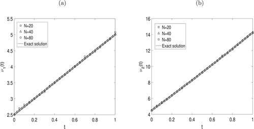
Table 1. The rmse values ((32(32) $\begin{array}{rl}rmse({\nu }_1)& ={[\frac{1}{N}\sum _{n=1}^N({\nu }_1^{Numerical}(t_n)-{\nu }_1^{Exact}(t_n){)}^2]}^{1/2},\end{array}$(32) ) and (33(33) $\begin{array}{rl}rmse({\nu }_2)& ={[\frac{1}{N}\sum _{n=1}^N({\nu }_2^{Numerical}(t_n)-{\nu }_2^{Exact}(t_n){)}^2]}^{1/2},\end{array}$(33) )) for ${\nu }_1(t)$ and ${\nu }_2(t)$, with $M_1=M_2=10$ and with various $N\in \{20,40,80\}$, for direct problem.

$M_1=M_2=10$	$rmse({\nu }_1)$	$rmse({\nu }_2)$
N = 20	0.0353	0.0479
N = 40	0.0080	0.0073
N = 80	0.0030	0.0026

Next we investigate the inverse problem. We fix $M_1=M_2=10$ and N = 40 and we start the investigation for reconstructing the unknown timewise thermal conductivity coefficients $a_1(t)$ and $a_2(t)$ and the temperature $u(x,y,t)$ for $p\in \{0,1\mathrm{\%},3\mathrm{\%},5\mathrm{\%}\}$ noise in the measured data (23(23) ${\nu }_1^{ϵ1}(t_n)={\nu }_1(t_n)+ϵ1_n,{\nu }_2^{ϵ2}(t_n)={\nu }_2(t_n)+ϵ2_n,n=\overline{0,N},$(23) ). We take the initial guesses for the vectors ${\mathbf{a}}_{\mathbf{1}}$ and ${\mathbf{a}}_{\mathbf{2}}$ as follows: (34) $a_1^0(t_n)=a_1(0)=1,a_2^0(t_n)=a_2(0)=1,n=\overline{1,N}.$(34) Note that the values of $a_1(0)$ and $a_2(0)$ are available from (22(22) $a_1(0)=\frac{{\nu }_1(0)}{{\phi }_x(0,Y_0)},a_2(0)=\frac{{\nu }_2(0)}{{\phi }_y(X_0,0)}.$(22) ). The objective function (19(19) $F({\mathbf{a}}_{\mathbf{1}},{\mathbf{a}}_{\mathbf{2}})=\sum _{n=1}^N[a_1^n{u}_x(0,Y_0,t_n)-{\nu }_1(t_n){]}^2+\sum _{n=1}^N[a_2^n{u}_y(X_0,0,t_n)-{\nu }_2(t_n){]}^2,$(19) ), as a function of the number of iterations, is plotted in Figure 3. From this figure, it can be seen that a fast monotonic decreasing convergence is achieved in about 5–9 iterations to reach a very low prescribed tolerance of $O({10}^{-26})$ in about 6 to 8 minutes CPU time. The corresponding numerical results for $a_1(t)$ and $a_2(t)$ are shown in Figure 4 and summarized in Table 2. From this figure and table, it can be seen that as the percentage of noise p decreases from $5\mathrm{\%}$ to $3\mathrm{\%}$ to $1\mathrm{\%}$ and then to zero the numerically obtained results becomes more stable and accurate. For more, information about the number of iterations, the values of the objective function (19) at final iteration, the rmse values ((26) and (27)) and the computational time, see Table 2. Figure 5 compares the analytical (30(30) $\begin{array}{rl}u(x,y,t)& =1+x+3y+3xy+t{x}^{2}y+\frac{1}{10}t{y}^3,(x,y,t)\in {\overline{Q}}_T,\end{array}$(30) ) and numerical solutions for $u(x,y,t)$ showing good agreement and stability. No regularization was found necessary to penalize the nonlinear least-squares objective functional (19) for amounts of noise up to $p=5\mathrm{\%}$, hinting towards the conclusion that the inverse problem under investigation is not severely ill-posed. Nevertheless, for higher amounts of noise the instability in retrieving the coefficients $a_1(t)$ and $a_2(t)$ will become apparent and regularization would need to be employed.

Figure 3. The objective function (19(19) $F({\mathbf{a}}_{\mathbf{1}},{\mathbf{a}}_{\mathbf{2}})=\sum _{n=1}^N[a_1^n{u}_x(0,Y_0,t_n)-{\nu }_1(t_n){]}^2+\sum _{n=1}^N[a_2^n{u}_y(X_0,0,t_n)-{\nu }_2(t_n){]}^2,$(19) ), as a function of the number of iterations, for Example 1 with $p\in \{0,1\mathrm{\%},3\mathrm{\%},5\mathrm{\%}\}$ noise.

Figure 4. The exact (31(31) $\begin{array}{rl}{a}_1(t)& =1+t,a_2(t)=1+2t,t\in [0,1].\end{array}$(31) ) and numerical solutions for: (a) $a_1(t)$ and (b) $a_2(t)$, for Example 1 with $p\in \{0,1\mathrm{\%},3\mathrm{\%},5\mathrm{\%}\}$ noise.

Figure 5. The analytical (30(30) $\begin{array}{rl}u(x,y,t)& =1+x+3y+3xy+t{x}^{2}y+\frac{1}{10}t{y}^3,(x,y,t)\in {\overline{Q}}_T,\end{array}$(30) ) and approximate solutions for the temperature $u(x,y,1)$, for Example 1 with (a) no noise, (b) $p=1\mathrm{\%}$ noise, (c) $p=3\mathrm{\%}$ noise, and (d) $p=5\mathrm{\%}$ noise. The absolute error between them is also included.

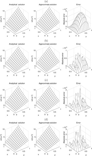
Table 2. The number of iterations, the values of the objective function (19) at final iteration, the rmse values ((26) and (27)) and the computational time, for $p\in \{0,1,3,5\}\mathrm{\%}$, for Examples 1 and 2.

Example 1	p = 0	$p=1\mathrm{\%}$	$p=3\mathrm{\%}$	$p=5\mathrm{\%}$
Number of iterations	9	9	5	5
Minimum value of (19)	8.6E−26	1.5E−25	1.7E−25	9.5E−26
$rmse(a_1)$	0.0013	0.0279	0.0836	0.1395
$rmse(a_2)$	0.0016	0.0286	0.0860	0.1434
Computational time	8 min	8 min	6 min	6 min
Example 2	p = 0	$p=1\mathrm{\%}$	$p=3\mathrm{\%}$	$p=5\mathrm{\%}$
Number of iterations	10	10	10	7
Minimum value of (19)	6.0E−26	5.5E−26	5.8E−26	1.0E−25
$rmse(a_1)$	0.0068	0.0285	0.0838	0.1396
$rmse(a_2)$	0.0039	0.0193	0.0574	0.0958
Computational time	9 min	9 min	9 min	7 min

5.2. Example 2

The previous example has recovered the smooth timewise thermal conductivity coefficients $a_1(t)$ and $a_2(t)$ as given in (31(31) $\begin{array}{rl}{a}_1(t)& =1+t,a_2(t)=1+2t,t\in [0,1].\end{array}$(31) ). In this example, we assess the numerical ADE scheme for reconstructing a non-smooth test: (35) $a_1(t)=1+{\cos }^2(2\pi t),a_2(t)=1+{\cos }^2(3\pi t),t\in [0,1].$(35) We also have the same analytical solution for the temperature $u(x,y,t)$ given by (30(30) $\begin{array}{rl}u(x,y,t)& =1+x+3y+3xy+t{x}^{2}y+\frac{1}{10}t{y}^3,(x,y,t)\in {\overline{Q}}_T,\end{array}$(30) ). The rest of the input data are the same as in Example 1 and (36) $\begin{array}{rl}{\nu }_1(t)& =\frac{5}{2}(1+{\cos }^2(2\pi t)),{\nu }_2(t)=\frac{1}{8}(18+t)(3+\cos (6\pi t)),\\ f(x,y,t)& =-(-1-t+3x+\frac{y}{100})(1+(3+2tx)y)+y(x^2+\frac{y^2}{10})\\ & -(-1-t+\frac{x}{100}+3y)(3+3x+t{x}^2+\frac{3t{y}^2}{10})\\ & -(-10+t+x+y)(1+x+3y+3xy+t{x}^{2}y+\frac{t{y}^3}{10})\\ & -t(1+x)y(3+\cos (4\pi t))-\frac{3}{10}ty(1+y)(3+\cos (6\pi t)).\end{array}$(36) Also, with this data, the conditions of Theorems 2.1 and 2.2 are fulfilled, hence the uniqueness of the solution is also guaranteed. The initial guesses for the vectors ${\mathbf{a}}_{\mathbf{1}}$ and ${\mathbf{a}}_{\mathbf{2}}$ for this example has been taken as (37) $a_1^0(t_n)=a_1(0)=2,a_2^0(t_n)=a_2(0)=2,n=\overline{1,N}.$(37) Note that the values of $a_1(0)$ and $a_2(0)$ are also available from (22(22) $a_1(0)=\frac{{\nu }_1(0)}{{\phi }_x(0,Y_0)},a_2(0)=\frac{{\nu }_2(0)}{{\phi }_y(X_0,0)}.$(22) ). We investigate the inverse problem as we did in Example 1. We take $M_1=M_2=10$ and N = 40 and reconstructing the unknown thermal conductivity coefficients $a_1(t)$ and $a_2(t)$ and the temperature $u(x,y,t)$ for exact and noisy measured input data (23(23) ${\nu }_1^{ϵ1}(t_n)={\nu }_1(t_n)+ϵ1_n,{\nu }_2^{ϵ2}(t_n)={\nu }_2(t_n)+ϵ2_n,n=\overline{0,N},$(23) ), for various amounts of noise p = 0 (no noise) and $p\in \{1\mathrm{\%},3\mathrm{\%},5\mathrm{\%}\}$ noisy data (24(24) ${\sigma }_1=p\times \underset{t\in [0,T]}{max}|{\nu }_1(t)|,{\sigma }_2=p\times \underset{t\in [0,T]}{max}|{\nu }_2(t)|,$(24) ). The objective function (19(19) $F({\mathbf{a}}_{\mathbf{1}},{\mathbf{a}}_{\mathbf{2}})=\sum _{n=1}^N[a_1^n{u}_x(0,Y_0,t_n)-{\nu }_1(t_n){]}^2+\sum _{n=1}^N[a_2^n{u}_y(X_0,0,t_n)-{\nu }_2(t_n){]}^2,$(19) ), as a function of the number of iterations, is plotted in Figure 6. From this figure one can notice that a rapid monotonically decreasing convergence is achieved in about 6–10 iterations, with the objective function reaching a very small value of $O({10}^{-26})$. The numerical results for the timewise thermal conductivity coefficients $a_1(t)$ and $a_2(t)$ are depicted in Figure 7 and summarized in Table 2. From this figure and table, it can be seen that as the percentage of noise p decreases from $5\mathrm{\%}$ to $3\mathrm{\%}$ to $1\mathrm{\%}$ and then to zero the numerically obtained results becomes more stable and accurate.

Figure 6. The objective function (19(19) $F({\mathbf{a}}_{\mathbf{1}},{\mathbf{a}}_{\mathbf{2}})=\sum _{n=1}^N[a_1^n{u}_x(0,Y_0,t_n)-{\nu }_1(t_n){]}^2+\sum _{n=1}^N[a_2^n{u}_y(X_0,0,t_n)-{\nu }_2(t_n){]}^2,$(19) ), as a function of the number of iterations, for Example 2 with $p\in \{0,1\mathrm{\%},3\mathrm{\%},5\mathrm{\%}\}$ noise.

Figure 7. The exact (35(35) $a_1(t)=1+{\cos }^2(2\pi t),a_2(t)=1+{\cos }^2(3\pi t),t\in [0,1].$(35) ) and numerical solutions for: (a) $a_1(t)$ and (b) $a_2(t)$, for Example 2 with $p\in \{0,1\mathrm{\%},3\mathrm{\%},5\mathrm{\%}\}$ noise.

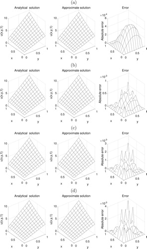
Finally, Figure 8 shows the analytical (35(35) $a_1(t)=1+{\cos }^2(2\pi t),a_2(t)=1+{\cos }^2(3\pi t),t\in [0,1].$(35) ) and numerical solutions for the temperature $u(x,y,t)$ for various amounts of noise $p\in \{0,1,3,5\}\mathrm{\%}$. From this figure it can be seen that the numerical solution is stable and furthermore, its accuracy improves as the noise level p decreases. The same conclusions can be drawn about the stable reconstructions for the unknown thermal conductivity coefficients.

Figure 8. The analytical (30(30) $\begin{array}{rl}u(x,y,t)& =1+x+3y+3xy+t{x}^{2}y+\frac{1}{10}t{y}^3,(x,y,t)\in {\overline{Q}}_T,\end{array}$(30) ) and approximate solutions for the temperature $u(x,y,1)$, for Example 2 with (a) no noise, (b) $p=1\mathrm{\%}$ noise, (c) $p=3\mathrm{\%}$ noise, and (d) $p=5\mathrm{\%}$ noise. The absolute error between them is also included.

6. Conclusions

In this paper, the inverse problem involving simultaneous identification of the timewise thermal conductivity coefficients $a_1(t)$ and $a_2(t)$ and the temperature $u(x,y,t)$ in the two-dimensional parabolic heat equation (1) in a rectangular domain from the local heat flux over-specification conditions (5) and (6) has been numerically investigated. The direct solver based on the ADE scheme is employed. The inverse problem approach based on a nonlinear least-squares minimization problem using the MATLAB optimization toolbox subroutine lsqnonlin is developed. The rmse values for various noise levels p for both smooth and non-smooth continuous timewise thermal diffusivity coefficients Examples were compared. Numerical results presented and discussed for both exact and noisy data show that accurate and stable solutions have been obtained. No regularization has been found necessary indicating that the inverse problem is not severely ill-posed. In principle, the numerical analysis of this paper can be extended to three-dimensional problems; however, this non-trivial investigation is deferred to future work.

Nomenclature

$a_1$	=	thermal conductivity (W m${}^{-1}$ K${}^{-1}$ )
$a_2$	=	thermal conductivity (W m${}^{-1}$ K${}^{-1}$ )
$c_1$	=	velocity (m s${}^{-1}$ )
$c_2$	=	velocity (m s${}^{-1}$ )
$c_3$	=	absorbance (AU)
f	=	heat source/force (J)
u	=	temperature (K or C)
${\nu }_1$	=	heat flux at x = 0 (W ${\mathrm{m}}^{-2}$ )
${\nu }_2$	=	heat flux at y = 0 (W ${\mathrm{m}}^{-2}$ )
t	=	time variable (s)
x, y	=	space variables (m)
$x_i,y_j$	=	space nodes (–)
$t_n$	=	time node (–)
$u_{i,j}^n$	=	values of u at the node $(i,j,n)$ (–)
l	=	end of space interval (–)
h	=	end of space interval (–)
T	=	end of time interval (–)
$M_1$	=	number of finite difference in x-coordinate (–)
$M_2$	=	number of finite difference in y-coordinate (–)
N	=	number of finite difference in t-coordinate (–)
F	=	nonlinear objective least-squares function (19) (–)
p	=	percentage of noise (–)
${\sigma }_1,{\sigma }_2$	=	standard deviations (–)
$Q_T$	=	fixed domain $(0,h)\times (0,l)\times (0,T)$ (–)
${\overline{Q}}_T$	=	closure of the solution domain $Q_T$ (–)

Acknowledgements

The comments and suggestions made by the editor and the referees are gratefully acknowledged.

Disclosure statement

No potential conflict of interest was reported by the author(s).

References

- Cannon JR, Yin HM. A class of nonlinear nonclassical parabolic equations. J Differ Equ. 1989;79:266–288. doi: 10.1016/0022-0396(89)90103-4
- Cannon JR, Matheson AL. A numerical procedure for diffusion subject to the specification of mass. Int J Eng Sci. 1993;31:347–355. doi: 10.1016/0020-7225(93)90010-R
- Cannon JR, Lin Y, Wang S. An implicit finite difference scheme for the diffusion equation subject to mass specification. Int J Eng Sci. 1990;28:573–578. doi: 10.1016/0020-7225(90)90086-X
- Ivanchov MI. Some inverse problems for the heat equation with nonlocal boundary condition. Ukrainian Math J. 1993;45:1066–1071. doi: 10.1007/BF01070965
- Ivanchov MI. On an inverse problem of heat conduction with nonlocal overdetermination condition. Visnyk L'vivskogo Universytetu Ser Mech Mat. 1994;40:12–15.
- Ivanchov MI. Inverse problems for equations of parabolic type. Liviv: VNTL; 2003.
- Huntul MJ, Lesnic D. Reconstruction of the timewise conductivity using a linear combination of heat flux measurements. J King Saud Univ Sci. 2020;32:928–933. doi: 10.1016/j.jksus.2019.05.006
- Huntul MJ, Lesnic D. An inverse problem of finding the time-dependent thermal conductivity from boundary data. Int Commun Heat Mass Transfer. 2017;85:147–154. doi: 10.1016/j.icheatmasstransfer.2017.05.009
- Huntul MJ, Hussein MS, Lesnic D, et al. Reconstruction of an orthotropic thermal conductivity. Int J Math Model Numer Optim. 2020;10:102–122.
- Alifanov OM, Budnik SA, Nenarokomov AV, et al. Estimation of thermal properties of materials with application for inflatable spacecraft structure testing. Inverse Probl Sci Eng. 2012;20:677–690. doi: 10.1080/17415977.2012.665909
- Huang CH, Huang CY. An inverse problem in estimating simultaneously the effective thermal conductivity and volumetric heat capacity of biological tissue. Appl Math Model. 2007;31:1785–1797. doi: 10.1016/j.apm.2006.06.002
- Mera NS, Elliott L, Ingham DB, et al. An iterative BEM for the Cauchy steady state heat conduction problem in an anisotropic medium with unknown thermal conductivity tensor. Inverse Prob Eng. 2000;8:579–607. doi: 10.1080/174159700088027748
- Reddy SR, Dulikravich GS. Simultaneous determination of spatially varying thermal conductivity and specific heat using boundary temperature measurements. Inverse Probl Sci Eng. 2019;27:1635–1649. doi: 10.1080/17415977.2019.1578352
- Reddy SR, Dulikravich GS, Zeidi SMJ. Non-destructive estimation of spatially varying thermal conductivity in 3D objects using boundary thermal measurements. Int J Thermal Sci. 2017;118:488–496. doi: 10.1016/j.ijthermalsci.2017.05.011
- Hussein MS, NSEP Kinash, Lesnic D, et al. Retrieving the time-dependent thermal conductivity of an orthotropic rectangular conductor. Appl Anal. 2017;96:1–15. doi: 10.1080/00036811.2016.1232401
- Sagaydak R. Large on existence and uniqueness of solution for the inverse problem of determination major coefficients in two-dimensional parabloic equation. Visnyk L'vivskogo Universytetu Ser Mech Mat. 2005;64:236–244.
- Barakat HZ, Clark AJ. On the solution of the diffusion equations by numerical methods. J Heat Transfer. 1966;88:421–427. doi: 10.1115/1.3691590
- Campbell LJ, Yin B. On the stability of alternating-direction explicit methods for advection-diffusion equations. Numer Meth Partial Differ Equ. 2007;23:1429–1444. doi: 10.1002/num.20233
- Ozisik MN. Finite difference methods in heat transfer. Boca Raton (FL): CRC Press; 1994.
- Mathworks. Documentation optimization toolbox-least squares (model fitting) algorithms; 2016. Available from: www.mathworks.com
- Coleman TF, Li Y. An interior trust region approach for nonlinear minimization subject to bounds. SIAM J Optim. 1996;6:418–445. doi: 10.1137/0806023
- Cannon JR. The one-dimensional heat equation. Menlo Park (CA): Addison-Wesley; 1984.