An efficient numerical method to solve inverse fuzzy-uncertain viscoelastic problems of identification

ABSTRACT

When there exists fuzzy uncertainty in experimentally determined information, viscoelastic constitutive parameters to be identified are treated as fuzzy variables, and a two-stage strategy cooperating with particle swarm method is presented to identify membership functions of fuzzy parameters. At each stage, inverse fuzzy problem is formulated as a series of α-level strategy-based inverse interval problems, which are described by optimization problems and are solved utilizing particle swarm method. Forward interval analysis required in inverse interval analysis is conducted by solving two optimization problems via modified coordinate search algorithm. To alleviate heavy computational burden, dimension-adaptive sparse grid (DSG) surrogate is embedded in optimization process. The surrogate is constructed on a solid platform of high fidelity deterministic solutions, which is provided by scaled boundary finite element method and temporally piecewise adaptive algorithm. Eventually, membership functions of fuzzy parameters can be obtained by fuzzy decomposition theorem with interval bounds acquired at each of α-sublevels. Parallelization is realized for construction of DSG surrogate and implementation of particle swarm method for a further computation reduction. Numerical examples are provided to illustrate effectiveness of proposed approach, where regional inhomogeneity and impact of measurement points selection on identification results are explored.

Keywords:

• Inverse viscoelastic problem
• fuzzy uncertainty
• scaled boundary finite element method
• piecewise adaptive computing
• sparse grid surrogate

2010 Mathematics Subject Classifications:

• 03E72
• 65M32
• 97N50

1. Introduction

The experiment-based identification of viscoelastic constitutive parameters is fundamental for the viscoelastic analysis and is an important issue related to a number of engineering aspects [1–8]. Nevertheless, the uncertainty in the experimentally determined information is inevitable [9], and causes an uncertainty in the constitutive parameters to be identified, which should be taken into account for the further reliable numerical analysis, and can be determined by solving the inverse uncertain problem of identification [10–12].

Probabilistic models and methods remain common practice to solve the inverse uncertain problems, where the uncertainties are quantified as random variables or stochastic processes by using a great amount of sample statistical information [13]. For example, Hernandez et al. [14] identified the properties of a viscoelastic tape using a probabilistic approach. Zhang et al. [15] addressed an inverse probabilistic approach to identify the frequency-dependent Young's modulus of the viscoelastic material in a laminated structure. Dosso and Holland [16] developed a nonlinear inverse probabilistic approach for seabed reflectivity data to estimate the viscoelastic parameters of upper sediments. Oates et al. [17] implemented stochastic-based optimization to identify the material parameters of a viscoelastic model.

However, the application of probabilistic theory often proves to be inconvenient in practice, because of the large amount of data necessary for the identification of probability density function or the corresponding statistical moments [18]. In contrast, non-probabilistic approaches can be alternatively used to treat uncertainties affecting material properties when only fragmentary or incomplete experimental data are available [19,20]. For instance, on the basis of evidence theory, Wang [21] proposed a framework of inverse analysis for the uncertain parameter identification in mechanical systems. Liu et al. investigated evidence theory-based methods for quantifying uncertainties with correlation [22] and without correlation [23]. On the basis of interval theory, Wang and Matthies [24] conducted an inverse interval analysis for the heat transfer problem with epistemic uncertainty. Wang et al. [25] developed a time domain-based method for the identification distributed dynamic load with interval uncertainties. On the base of fuzzy theory, Wang et al. also developed methodologies of reliability-based multidisciplinary design optimization with fuzzy uncertainty [26], and with hybrid interval and fuzzy uncertainties [27]. As a non-probabilistic uncertainty model, the fuzzy approach gives a measure for the sensitivity of the design boundaries and is useful in an early design phase where some model properties are only known vaguely [28]. However, the inverse fuzzy uncertainty quantification has only been introduced very recently [28]. Wang et al. [13] carried out the identification of membership functions of fuzzy modelling parameters for the steady-state heat transfer problem. Erdogan and Bakir [9] carried out an inverse finite element analysis to determine the membership functions of the fuzzy updating parameters for the damage detection problem. Haag et al. [29] proposed inverse fuzzy arithmetic to identify the uncertain damping and material parameters for a brake pad with a single or multiple measurements. Hanss et al. [30] identified the fuzzy-valued stiffness and damping parameters from measured data of the eigenfrequencies and the damping ratio for a bolted joint model. But there seems no report directly related to the inverse fuzzy viscoelastic problems.

Nearly all the inverse fuzzy analyses are transformed into a series of inverse interval analyses by utilizing the α-level strategy [28], which are usually conducted by solving a series of optimization problems and involve an amount of forward interval analysis. For the bounds estimation in the forward interval analysis, optimization techniques are reliable no matter the interval scales are large or small [28], but usually bear a heavy computational burden caused by the repeated deterministic solutions or sensitivity analysis [31–34], particularly for the nonlinear or time-dependent problems. On the other hand, a sufficient solution accuracy is required in the deterministic analysis.

With the aforementioned considerations, a two-stage strategy cooperating with the particle swarm method is put forward to identify the membership functions of fuzzy viscoelastic constitutive parameters. At each stage, the inverse fuzzy problem is solved via a series of α-level strategy-based inverse interval problems, in which the lower and upper bounds of viscoelastic constitutive parameters are identified simultaneously by solving an optimization problem utilizing the particle swarm method [35–37]. The forward interval analysis required in the α-level strategy-based inverse interval analysis is conducted by solving two optimization problems via a modified coordinate search algorithm [38]. To alleviate the heavy computational burden in the above optimization process, an economic surrogate with sufficient accuracy is constructed to approximate the expensive deterministic time-dependent solutions of viscoelastic problems and is mingled with the modified coordinate search algorithm. The surrogate is constructed by a dimension-adaptive sparse grid (DSG) technique with piecewise multilinear basis functions [39] and is based upon a solid platform of high fidelity deterministic solution of viscoelastic problems, which is provided by the scaled boundary finite element method (SBFEM) [40] and a temporally piecewise adaptive algorithm (TPAA) [41,42]. SBFEM is semi-analytical, and the TPAA takes advantage of accurate and stable solution accuracy when the step size varies. Subsequently, the membership functions of the viscoelastic constitutive parameters can be determined by a fuzzy decomposition theorem [13,43] with the interval bounds acquired at each of α-sublevels. The parallelization is realized for the construction of surrogate and the implementation of the particle swarm method for a further reduction of computational expense. Numerical examples are provided to illustrate the effectiveness of the proposed approach, and the regional inhomogeneity and the impacts of temporal and spatial selections of measurement points on the identification results are taken into account.

The remainder of this paper is organized as follows: Section 2 presents the basic equations for the solution of deterministic forward viscoelastic problems. Subsequently, the construction of DSG surrogate and the DSG-based bounds estimation are described in Section 3. Then, the solution process of inverse fuzzy viscoelastic problems is given in Section 4. Numerical examples are provided in Section 5 to illustrate the effectiveness of the proposed method. Finally, Section 6 goes to the conclusions.

2. Basic equations for the solution of deterministic forward viscoelastic problems

2.1. Governing and recursive governing equations

The governing equations of viscoelastic problems are written as [44] (1) $\begin{array}{rl}& \mathbf{H}\mathit{\sigma }+\mathbf{b}=\mathbf{0}\mathrm{in}\mathrm{\Omega },\end{array}$(1) (2) $\begin{array}{rl}& \mathit{\epsilon }={\mathbf{H}}^{\mathrm{T}}\mathbf{u}\mathrm{in}\mathrm{\Omega },\end{array}$(2) (3) $\begin{array}{rl}& \mathbf{H}=\left[\begin{array}{ccc}{\displaystyle \frac{\mathrm{\partial }}{\mathrm{\partial }x}}& 0& {\displaystyle \frac{\mathrm{\partial }}{\mathrm{\partial }y}}\\ 0& {\displaystyle \frac{\mathrm{\partial }}{\mathrm{\partial }y}}& {\displaystyle \frac{\mathrm{\partial }}{\mathrm{\partial }y}}\end{array}\right],\end{array}$(3) where $\mathit{\sigma }$ and $\mathit{ϵ}$ represent the vectors of stress and strain, respectively. $\mathbf{b}$ is the vector of body force intensity. Ω denotes the spatial domain of interest. $\mathbf{u}$ is the vector of displacement. $(\bullet {)}^{\mathrm{T}}$ denotes the transpose of •. x and y denote the Cartesian coordinates.

The boundary conditions are specified by [44] (4) $\begin{array}{rl}\mathbf{u}& ={\mathbf{u}}_b\mathrm{on}{\mathrm{\Gamma }}_u,\end{array}$(4) (5) $\begin{array}{rl}\mathbf{p}& ={\mathbf{p}}_b\mathrm{on}{\mathrm{\Gamma }}_{\sigma },\end{array}$(5) where $\mathbf{p}$ denotes the vector of traction. ${\mathbf{u}}_b$ and ${\mathbf{p}}_b$ are the prescribed values of $\mathbf{u}$ and $\mathbf{p}$ on the displacement and stress boundary, respectively. $\mathrm{\Gamma }={\mathrm{\Gamma }}_u+{\mathrm{\Gamma }}_{\sigma }$ stands for the whole boundary of Ω, and the subscripts u and σ refer to the displacement and stress, respectively.

We divide the time domain into a number of intervals where the initial points and the sizes of intervals are defined by $t_0,t_1,t_2,\dots ,t_k,\dots$ and $T_1,T_2,\dots ,T_k,\dots$, respectively. At the kth discretized time interval, in order to describe the variation of variables more precisely, all variables are expanded in terms of s (6) $\begin{array}{rl}& \mathit{\sigma }=\sum _{m=0}{\mathit{\sigma }}^m{s}^m,\end{array}$(6) (7) $\begin{array}{rl}& \mathit{\epsilon }=\sum _{m=0}{\mathit{\epsilon }}^m{s}^m,\end{array}$(7) (8) $\begin{array}{rl}& \mathbf{b}=\sum _{m=0}{\mathbf{b}}^m{s}^m,\end{array}$(8) (9) $\begin{array}{rl}& \mathbf{u}=\sum _{m=0}{\mathbf{u}}^m{s}^m,\end{array}$(9) (10) $\begin{array}{rl}& {\mathbf{u}}_b=\sum _{m=0}{\mathbf{u}}_b^m{s}^m,\end{array}$(10) (11) $\begin{array}{rl}& \mathbf{p}=\sum _{m=0}{\mathbf{p}}^m{s}^m,\end{array}$(11) (12) $\begin{array}{rl}& {\mathbf{p}}_b=\sum _{m=0}{\mathbf{p}}_b^m{s}^m,\end{array}$(12) (13) $\begin{array}{rl}& s=\frac{t-t_{k-1}}{T_k},\end{array}$(13) where ${\mathit{\sigma }}^m$, ${\mathit{\epsilon }}^m$, ${\mathbf{b}}^{\mathbf{m}}$, ${\mathbf{u}}^{\mathbf{m}}$, ${\mathbf{u}}_b^m$, ${\mathbf{p}}^{\mathbf{m}}$ and ${\mathbf{p}}_b^m$ $(m=0,1,2,\dots )$ represent the expansion coefficients of $\mathit{\sigma }$, $\mathit{\epsilon }$, $\mathbf{b}$, $\mathbf{u}$, ${\mathbf{u}}_b$, $\mathbf{p}$ and ${\mathbf{p}}_b$, respectively. t refers to time.

Substituting Equations (6(6) $\begin{array}{rl}& \mathit{\sigma }=\sum _{m=0}{\mathit{\sigma }}^m{s}^m,\end{array}$(6) )–(12(12) $\begin{array}{rl}& {\mathbf{p}}_b=\sum _{m=0}{\mathbf{p}}_b^m{s}^m,\end{array}$(12) ) into Equations (1(1) $\begin{array}{rl}& \mathbf{H}\mathit{\sigma }+\mathbf{b}=\mathbf{0}\mathrm{in}\mathrm{\Omega },\end{array}$(1) )–(5(5) $\begin{array}{rl}\mathbf{p}& ={\mathbf{p}}_b\mathrm{on}{\mathrm{\Gamma }}_{\sigma },\end{array}$(5) ) and equating the power of two sides of equations then yields (14) $\begin{array}{rl}& \mathbf{H}{\mathit{\sigma }}^m+{\mathbf{b}}^m=\mathbf{0}\mathrm{in}\mathrm{\Omega },\end{array}$(14) (15) $\begin{array}{rl}& {\mathit{\epsilon }}^m={\mathbf{H}}^{\mathrm{T}}{\mathbf{u}}^m\mathrm{in}\mathrm{\Omega },\end{array}$(15) (16) $\begin{array}{rl}& {\mathbf{u}}^m={\mathbf{u}}_b^m\mathrm{on}{\mathrm{\Gamma }}_u,\end{array}$(16) (17) $\begin{array}{rl}& {\mathbf{p}}^m={\mathbf{p}}_b^m\mathrm{on}{\mathrm{\Gamma }}_{\sigma }.\end{array}$(17)

2.2. Constitutive and recursive constitutive equations

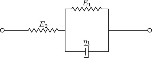
The constitutive equations of viscoelastic problems are described by a three-parameter solid viscoelastic model (Figure 1) in a differential form [45] (18) $\begin{array}{rl}& \mathit{\sigma }+{\alpha }_2\frac{\mathrm{\partial }\mathit{\sigma }}{\mathrm{\partial }t}=\mathbf{D}({\alpha }_1\mathit{\epsilon }+{\alpha }_2\frac{\mathrm{\partial }\mathit{\epsilon }}{\mathrm{\partial }t})(t>0),\end{array}$(18) (19) $\begin{array}{rl}& \mathit{\sigma }=\mathbf{D}\mathit{\epsilon }(t=0),\end{array}$(19) where (20) ${\alpha }_1=\frac{E_1}{E_1+E_2},{\alpha }_2=\frac{{\eta }_1}{E_1+E_2}.$(20) $E_1$ and $E_2$ indicate the moduli of elasticity. ${\eta }_1$ is the material coefficient of viscosity.

Figure 1. Three-parameter solid model of viscoelastic material.

For the plane stress problems, $\mathbf{D}$ is given by (21) $\mathbf{D}=\frac{E_2}{1-v^2}\left[\begin{array}{ccc}1& v& 0\\ v& 1& 0\\ 0& 0& {\displaystyle \frac{1-v}{2}}\end{array}\right]=E_2{\mathbf{D}}_0,$(21) where (22) ${\mathbf{D}}_0=\frac{1}{1-v^2}\left[\begin{array}{ccc}1& v& 0\\ v& 1& 0\\ 0& 0& {\displaystyle \frac{1-v}{2}}\end{array}\right].$(22) v is Poisson's ratio.

For the plane strain problems, $E_1$, $E_2$ and v need to be replaced by $E_1/(1-v^2)$, $E_2/(1-v^2)$ and $v/(1-v)$, respectively.

Because (23) $\frac{\mathrm{d}(\bullet )}{\mathrm{d}t}=\frac{1}{T_k}\frac{\mathrm{d}(\bullet )}{\mathrm{d}s}.$(23) Therefore, (24) $\begin{array}{rl}& \frac{\mathrm{\partial }\mathit{\sigma }}{\mathrm{\partial }t}=\sum _{m=0}\frac{m+1}{T_k}{\mathit{\sigma }}^{(m+1)}{s}^m,\end{array}$(24) (25) $\begin{array}{rl}& \frac{\mathrm{\partial }\mathit{\epsilon }}{\mathrm{\partial }t}=\sum _{m=0}\frac{m+1}{T_k}{\mathit{\epsilon }}^{(m+1)}{s}^m.\end{array}$(25) Substituting Equations (6(6) $\begin{array}{rl}& \mathit{\sigma }=\sum _{m=0}{\mathit{\sigma }}^m{s}^m,\end{array}$(6) ), (7(7) $\begin{array}{rl}& \mathit{\epsilon }=\sum _{m=0}{\mathit{\epsilon }}^m{s}^m,\end{array}$(7) ), (24(24) $\begin{array}{rl}& \frac{\mathrm{\partial }\mathit{\sigma }}{\mathrm{\partial }t}=\sum _{m=0}\frac{m+1}{T_k}{\mathit{\sigma }}^{(m+1)}{s}^m,\end{array}$(24) ) and (25(25) $\begin{array}{rl}& \frac{\mathrm{\partial }\mathit{\epsilon }}{\mathrm{\partial }t}=\sum _{m=0}\frac{m+1}{T_k}{\mathit{\epsilon }}^{(m+1)}{s}^m.\end{array}$(25) ) into Equations (18(18) $\begin{array}{rl}& \mathit{\sigma }+{\alpha }_2\frac{\mathrm{\partial }\mathit{\sigma }}{\mathrm{\partial }t}=\mathbf{D}({\alpha }_1\mathit{\epsilon }+{\alpha }_2\frac{\mathrm{\partial }\mathit{\epsilon }}{\mathrm{\partial }t})(t>0),\end{array}$(18) ) and (19(19) $\begin{array}{rl}& \mathit{\sigma }=\mathbf{D}\mathit{\epsilon }(t=0),\end{array}$(19) ), and equating the power of two sides of the equation then gives (26) $\begin{array}{rl}& {\mathit{\sigma }}^m=\mathbf{D}{\mathit{\epsilon }}^m+{\mathbf{C}}^m,\end{array}$(26) (27) $\begin{array}{rl}& {\mathbf{C}}^m=\frac{T_k}{m}(\frac{E_1}{{\eta }_1}\mathbf{D}{\mathit{\epsilon }}^{m-1}-\frac{1}{{\alpha }_2}{\mathit{\sigma }}^{m-1})(m>0),\end{array}$(27) (28) $\begin{array}{rl}& {\mathbf{C}}^0=\mathbf{0}(k=1),\end{array}$(28) (29) $\begin{array}{rl}& {\left\{{\mathbf{C}}^0\right\}}_{(k+1)}={\left\{\sum _{m=0}{\mathbf{C}}^m\right\}}_k(k>1).\end{array}$(29) At the first time interval (30) ${\mathit{\sigma }}^0=\mathbf{D}{\mathit{\epsilon }}^0.$(30) At the $(k+1)$th time interval (31) $\{\begin{array}{l}{\left\{{\mathit{\sigma }}^0\right\}}_{(k+1)}={\displaystyle \sum _{m=0}{\left\{{\mathit{\sigma }}^m\right\}}_k,}\\ {\left\{{\mathit{\epsilon }}^0\right\}}_{(k+1)}={\displaystyle \sum _{m=0}{\left\{{\mathit{\epsilon }}^m\right\}}_k,}\end{array}k=1,2,3,\dots ,$(31) where the subscripts $(k+1)$ and k refer to the $(k+1)$th and kth time intervals, respectively.

2.3. Recursive SBFEM equations of solving deterministic forward problems

In the absence of body force, the application of virtual work principle on Equations (14(14) $\begin{array}{rl}& \mathbf{H}{\mathit{\sigma }}^m+{\mathbf{b}}^m=\mathbf{0}\mathrm{in}\mathrm{\Omega },\end{array}$(14) )–(17(17) $\begin{array}{rl}& {\mathbf{p}}^m={\mathbf{p}}_b^m\mathrm{on}{\mathrm{\Gamma }}_{\sigma }.\end{array}$(17) ) over the whole domain gives [40] (32) $\sum _e{\int }_{{\mathrm{\Omega }}_e}\delta {\mathit{\epsilon }}^{\mathrm{T}}{\mathit{\sigma }}^m\mathrm{d}{\mathrm{\Omega }}_e=\sum _l{\int }_{{\mathrm{\Gamma }}_l}\delta {\mathbf{u}}^{\mathrm{T}}{\mathbf{p}}^m\mathrm{d}{\mathrm{\Gamma }}_l,$(32) where the second term refers to a sum of the virtual work generated by tractions at each piece along ${\mathrm{\Gamma }}_{\sigma }$. ${\mathrm{\Gamma }}_l$ refers to the length of lth piece along ${\mathrm{\Gamma }}_{\sigma }$. ${\mathrm{\Omega }}_e$ stands for the domain of eth element of SBFEM. $\delta \mathit{\epsilon }$ and $\delta \mathbf{u}$ are the vectors of virtual strain and displacement, respectively.

In light of Equations (26(26) $\begin{array}{rl}& {\mathit{\sigma }}^m=\mathbf{D}{\mathit{\epsilon }}^m+{\mathbf{C}}^m,\end{array}$(26) )–(29(29) $\begin{array}{rl}& {\left\{{\mathbf{C}}^0\right\}}_{(k+1)}={\left\{\sum _{m=0}{\mathbf{C}}^m\right\}}_k(k>1).\end{array}$(29) ) and (32(32) $\sum _e{\int }_{{\mathrm{\Omega }}_e}\delta {\mathit{\epsilon }}^{\mathrm{T}}{\mathit{\sigma }}^m\mathrm{d}{\mathrm{\Omega }}_e=\sum _l{\int }_{{\mathrm{\Gamma }}_l}\delta {\mathbf{u}}^{\mathrm{T}}{\mathbf{p}}^m\mathrm{d}{\mathrm{\Gamma }}_l,$(32) ), an SBFEM equation can be derived [46] (33) $\begin{array}{rl}& \mathbf{K}{\mathbf{d}}^m={\mathbf{P}}^m,\end{array}$(33) (34) $\begin{array}{rl}& \mathbf{K}=\sum _e{\mathbf{M}}_e^{\mathrm{T}}{\mathbf{K}}_e{\mathbf{M}}_e,\end{array}$(34) (35) $\begin{array}{rl}& {\mathbf{K}}_e={\int }_{{\mathrm{\Omega }}_e}{\mathbf{B}}^{\mathrm{T}}{\mathbf{D}}^{\mathrm{e}}\mathbf{B}\mathrm{d}{\mathrm{\Omega }}_e={\int }_{{\mathrm{\Omega }}_e}{E}_2^e{\mathbf{B}}^{\mathrm{T}}{\mathbf{D}}_0^e\mathbf{B}\mathrm{d}{\mathrm{\Omega }}_e,\end{array}$(35) (36) $\begin{array}{rl}& {\mathbf{P}}^m=\mathbf{P}{\mathbf{S}}^m+{\mathbf{P}\mathbf{C}}^m,\end{array}$(36) (37) $\begin{array}{rl}& \mathbf{P}{\mathbf{S}}^m=\sum _l({\mathbf{M}}_l{)}^{\mathrm{T}}{\int }_{{\mathrm{\Gamma }}_l}{\mathbf{N}}^{\mathrm{T}}{\mathbf{p}}^m\mathrm{d}{\mathrm{\Gamma }}_l,\end{array}$(37) (38) $\begin{array}{rl}& \mathbf{P}{\mathbf{C}}^m=\sum _e\frac{T_k}{m}{\mathbf{M}}_e^{\mathrm{T}}(-\frac{E_2^e}{{\eta }_1^e}{\mathbf{K}}_e{\mathbf{d}}_e^{m-1}-\frac{E_1^e+E_2^e}{{\eta }_1^e}{\mathbf{P}\mathbf{C}}_e^{m-1}),\end{array}$(38) (39) $\begin{array}{rl}& {\mathbf{P}\mathbf{C}}_e^{m-1}={\int }_{{\mathrm{\Omega }}_{\mathrm{e}}}{\mathbf{B}}^{\mathrm{T}}{\mathbf{C}}_e^{m-1}\mathrm{d}{\mathrm{\Omega }}_{\mathrm{e}},\end{array}$(39) (40) $\begin{array}{rl}& {\mathbf{P}\mathbf{C}}^0=\mathbf{0}(k=1),\end{array}$(40) (41) $\begin{array}{rl}& {\left\{{\mathbf{P}\mathbf{C}}^0\right\}}_{(k+1)}=\sum _{m=0}{\left\{\mathbf{P}{\mathbf{C}}^m\right\}}_k,\end{array}$(41) where ${\mathbf{d}}^m$ refers to a coefficient of $\mathbf{d}=\sum _{m=0}{\mathbf{d}}_{}^m{s}^m$ which denotes the global nodal vector of displacement. ${\mathbf{d}}_e^m$ refers to a coefficient of ${\mathbf{d}}_e=\sum _{m=0}{\mathbf{d}}_e^m{s}^m$ which denotes a nodal vector of displacement at the element level. ${\mathbf{M}}_e$ is a matrix mapping the degree of freedom (DOF) from the eth element to the global system, and ${\mathbf{M}}_l$ refers to a matrix mapping the DOF from the lth piece to the global system. $\mathbf{N}$ refers to a shape function. $\mathbf{B}={\mathbf{H}}^{\mathrm{T}}\mathbf{N}$. ${\mathbf{C}}_e^{m-1},{\mathbf{D}}^e,{\mathbf{D}}_0^e,E_1^e,E_2^e$ and ${\eta }_1^e$ refer to ${\mathbf{C}}^{m-1},\mathbf{D},{\mathbf{D}}_0,E_1,E_2$ and ${\eta }_1$ at the eth element of SBFEM, respectively. ${\mathbf{K}}_e$ stands for the stiffness matrix of eth element of SBFEM which is given in Appendix.

At the initial points of kth time interval, ${\mathbf{d}}^0$ is determined by (42) $\begin{array}{rl}& {\left\{{\mathbf{d}}^0\right\}}_k={\mathbf{K}}^{-1}\mathbf{P}{\mathbf{S}}^0\mathrm{if}k=1,\end{array}$(42) (43) $\begin{array}{rl}& {\left\{{\mathbf{d}}^0\right\}}_k=\sum _{m=0}{\left\{{\mathbf{d}}^m\right\}}_{(k-1)}\mathrm{if}k>1.\end{array}$(43) An adaptive computing process at a time interval can be realized with the increase of m until the following criteria is satisfied: (44) $\frac{{\Vert {{\mathbf{d}}^m{s}^m|}_{s=1}\Vert }_2}{{\Vert {\sum _{j=0}^{m-1}{\mathbf{d}}^j{s}^j|}_{s=1}\Vert }_2}\le \beta ,$(44) where β is a prescribed error tolerance and $\Vert \bullet {\Vert }_2$ represents a $L^2$ -norm.

Equation (44(44) $\frac{{\Vert {{\mathbf{d}}^m{s}^m|}_{s=1}\Vert }_2}{{\Vert {\sum _{j=0}^{m-1}{\mathbf{d}}^j{s}^j|}_{s=1}\Vert }_2}\le \beta ,$(44) ) is checked when each ${\mathbf{d}}^m$ is obtained. If it is satisfied, the computation at the current time interval will stop and step into the next time interval.

3. Bounds estimation at an α-sublevel

Nearly all the inverse fuzzy analyses are transformed into a series of inverse interval analyses by utilizing the α-level strategy [28]. In each of the inverse interval analyses, an amount of forward interval analysis is required.

Assume that there are N subdomains, and each of subdomains has n fuzzy viscoelastic constitutive parameters. All membership functions of fuzzy parameters are divided into M + 1 α-sublevels by the α-level strategy.

At jth α-sublevel $(j=0,1,2,\dots ,M)$, ${\underset{\_}{\mathbf{d}}}^{(j)}$ and ${\overline{\mathbf{d}}}^{(j)}$ (the lower and upper bounds of $\mathbf{d}$ at jth α-sublevel) can be obtained by the optimization technique which is reliable for the bounds estimation of interval problems [28]. In order to reduce the computational expense caused by repeated deterministic solutions in the optimization process, a DSG surrogate with piecewise multilinear basis functions [39] is developed to approximate the deterministic forward solutions of viscoelastic problems and is cooperated with the modified coordinate search algorithm [38] to estimate ${\underset{\_}{\mathbf{d}}}^{(j)}$ and ${\overline{\mathbf{d}}}^{(j)}$ with sufficient accuracy and a lower computational cost.

3.1. DSG surrogate

Sparse grid (SG) surrogate with piecewise multilinear basis functions can provide a good compromise between the accuracy and computational cost, and requires fewer support nodes than conventional surrogate on the full grid [39]. The DSG surrogate is an SG surrogate equipped with the dimension-adaptive technique so as to further reduce the computational effort [39].

Following the work given by Klimke [39], a DSG surrogate is constructed to approximate the solution of forward deterministic viscoelastic problems, and the piecewise multilinear function [39,47] is utilized as the basis function and Chebyshev-distributed sample points [48] are used in the DSG construction. The approximate solution of DSG is defined by $A(\mathbf{d}(\mathbf{I},t))$ where $\mathbf{I}$ refers to a vector of viscoelastic constitutive parameters. $A(\mathbf{d}(\mathbf{I},t))$ represents an approximate relationship between $\mathbf{d}$ and viscoelastic constitutive parameters within their definition regions in the whole time domain.

3.2. DSG-based bounds estimation

DSG-based bounds estimation at jth α-sublevel can be conducted via (45) $\begin{array}{rl}& {\underset{\_}{\mathbf{d}}}^{(j)}=\underset{\mathbf{x}\in {\mathrm{\Omega }}_1^{(j)}\times {\mathrm{\Omega }}_2^{(j)}\times \cdots \times {\mathrm{\Omega }}_N^{(j)}}{min}A(\mathbf{d}(\mathbf{I},t))(\mathbf{x}),\end{array}$(45) (46) $\begin{array}{rl}& {\overline{\mathbf{d}}}^{(j)}=\underset{\mathbf{x}\in {\mathrm{\Omega }}_1^{(j)}\times {\mathrm{\Omega }}_2^{(j)}\times \cdots \times {\mathrm{\Omega }}_N^{(j)}}{max}A(\mathbf{d}(\mathbf{I},t))(\mathbf{x}),\end{array}$(46) where ${\mathrm{\Omega }}_g^{(j)}=(I_1^{(j)}{)}_g\times (I_2^{(j)}{)}_g\cdots \times (I_n^{(j)}{)}_g$ denotes a n-dimensional box formed by the Cartesian product of $(I_i^{(j)}{)}_g$ which stands for the interval bounds of the ith fuzzy input parameter at the jth α-sublevel and gth subdomain [39,49]. $(I_i^{(j)}{)}_g=[({\underset{\_}{I}}_i^{(j)}{)}_g({\overline{I}}_i^{(j)}{)}_g]$. $({\underset{\_}{I}}_i^{(j)}{)}_g$ and $({\overline{I}}_i^{(j)}{)}_g$ refer to the lower and upper bounds of $(I_i^{(j)}{)}_g$, respectively. $i=1,2,\dots ,n$. $g=1,2,\dots ,N$. Equations (45(45) $\begin{array}{rl}& {\underset{\_}{\mathbf{d}}}^{(j)}=\underset{\mathbf{x}\in {\mathrm{\Omega }}_1^{(j)}\times {\mathrm{\Omega }}_2^{(j)}\times \cdots \times {\mathrm{\Omega }}_N^{(j)}}{min}A(\mathbf{d}(\mathbf{I},t))(\mathbf{x}),\end{array}$(45) ) and (46(46) $\begin{array}{rl}& {\overline{\mathbf{d}}}^{(j)}=\underset{\mathbf{x}\in {\mathrm{\Omega }}_1^{(j)}\times {\mathrm{\Omega }}_2^{(j)}\times \cdots \times {\mathrm{\Omega }}_N^{(j)}}{max}A(\mathbf{d}(\mathbf{I},t))(\mathbf{x}),\end{array}$(46) ) are solved by the modified coordinate search algorithm [38].

4. The solution process of inverse fuzzy viscoelastic problems

Assume $({\tilde{E}}_1{)}_g,({\tilde{E}}_2{)}_g,({\tilde{\eta }}_1{)}_g$ and $(\tilde{v}{)}_g$ refer to the fuzzy viscoelastic constitutive parameters at the gth subdomain. In light of Equations (33(33) $\begin{array}{rl}& \mathbf{K}{\mathbf{d}}^m={\mathbf{P}}^m,\end{array}$(33) )–(41(41) $\begin{array}{rl}& {\left\{{\mathbf{P}\mathbf{C}}^0\right\}}_{(k+1)}=\sum _{m=0}{\left\{\mathbf{P}{\mathbf{C}}^m\right\}}_k,\end{array}$(41) ), it is noted that $({\tilde{E}}_1{)}_g$ and $({\tilde{\eta }}_1{)}_g$ only relate to the right-hand side of Equation (33(33) $\begin{array}{rl}& \mathbf{K}{\mathbf{d}}^m={\mathbf{P}}^m,\end{array}$(33) ), while Equation (42(42) $\begin{array}{rl}& {\left\{{\mathbf{d}}^0\right\}}_k={\mathbf{K}}^{-1}\mathbf{P}{\mathbf{S}}^0\mathrm{if}k=1,\end{array}$(42) ) only relates to $({\tilde{E}}_2{)}_g$ and $(\tilde{v}{)}_g$ when t = 0. Therefore, a two-stage strategy is presented to identify the membership functions of unknown fuzzy viscoelastic constitutive parameters.

Stage 1. Estimate the membership functions of $({\tilde{E}}_2{)}_g$ and $(\tilde{v}{)}_g$ with $(E_2^{(j)}{)}_g$ $({\overline{E}}_2^{(j)}{)}_g,({\underset{\_}{v}}^{(j)}{)}_g$ and $({\overline{v}}^{(j)}{)}_g$ obtained by solving a series of inverse interval problems. $({\underset{\_}{E}}_2^{(j)}{)}_g,({\overline{E}}_2^{(j)}{)}_g,({\underset{\_}{v}}^{(j)}{)}_g$ and $({\overline{v}}^{(j)}{)}_g$ stand for the lower and upper bounds of $({\tilde{E}}_2{)}_g$ and $(\tilde{v}{)}_g$ at the jth α-sublevel, respectively. In this stage, we only need the fuzzy measurements of displacement at t = 0.

Stage 2. Estimate the membership functions of $({\tilde{E}}_1{)}_g$ and $({\tilde{\eta }}_1{)}_g$ with $(E_1^{(j)}{)}_g$, $({\overline{E}}_1^{(j)}{)}_g,({\underset{\_}{\eta }}_1^{(j)}{)}_g$ and $({\overline{\eta }}_1^{(j)}{)}_g$ obtained by solving a series of inverse interval problems. $(E_1^{(j)}{)}_g,({\overline{E}}_1^{(j)}{)}_g,({\underset{\_}{\eta }}_1^{(j)}{)}_g$ and $({\overline{\eta }}_1^{(j)}{)}_g$ stand for lower and upper bounds of $({\tilde{E}}_1{)}_g$ and $({\tilde{\eta }}_1{)}_g$ at the jth α-sublevel. In this stage, we only need the fuzzy measurements of displacement at t>0.

Let (47) ${\mathit{\phi }}^{(j)}={\{{\mathit{\phi }}_1^{(j)},{\mathit{\phi }}_2^{(j)},\dots ,{\mathit{\phi }}_N^{(j)}\}}^{\mathrm{T}}.$(47) At the first stage, (48) ${\mathit{\phi }}_g^{(j)}=\{({\underset{\_}{E}}_2^{(j)}{)}_g,({\overline{E}}_2^{(j)}{)}_g,({\underset{\_}{v}}^{(j)}{)}_g,({\overline{v}}^{(j)}{)}_g\},g=1,2,\dots ,N.$(48) At the second stage, (49) ${\mathit{\phi }}_g^{(j)}=\{({\underset{\_}{E}}_1^{(j)}{)}_g,({\overline{E}}_1^{(j)}{)}_g,({\underset{\_}{\eta }}_1^{(j)}{)}_g,({\overline{\eta }}_1^{(j)}{)}_g\}.$(49) Let ${\tilde{\mathrm{\Lambda }}}_{k,l}$ denotes the fuzzy measurements of displacement where the subscripts k and l refer to the kth spatial point and lth temporal point, respectively.

Utilizing the α-level strategy (Figure 2), fuzzy numbers of ${\tilde{\mathrm{\Lambda }}}_{k,l}$ is decomposed into a set of M + 1 intervals [50] (50) ${\mathbf{D}}_{\ast }=\{[{\underset{\_}{\mathrm{\Lambda }}}_{k,l}^{(0)},{\overline{\mathrm{\Lambda }}}_{k,l}^{(0)}],[{\underset{\_}{\mathrm{\Lambda }}}_{k,l}^{(1)},{\overline{\mathrm{\Lambda }}}_{k,l}^{(1)}],\dots ,[{\underset{\_}{\mathrm{\Lambda }}}_{k,l}^{(M)},{\overline{\mathrm{\Lambda }}}_{k,l}^{(M)}]\}.$(50) ${\mathit{\phi }}^{(j)}$ can be obtained by solving an optimization problem defined by (51) $\begin{array}{rl}& \mathrm{Seek}{\mathit{\phi }}^{(j)}\end{array}$(51) (52) $\begin{array}{rl}& \mathrm{Via}min\prod =\sum _k\sum _l\frac{1}{2}\left({\underset{\_}{U}}_{k,l}^2+{\overline{U}}_{k,l}^2\right)\end{array}$(52) (53) $\begin{array}{rl}& {\underset{\_}{U}}_{k,l}={\underset{\_}{d}}_{k,l}^{(j)}({\mathit{\phi }}^{(j)})-{\underset{\_}{\mathrm{\Lambda }}}_{k,l}^{(j)},\end{array}$(53) (54) $\begin{array}{rl}& {\overline{U}}_{k,l}={\overline{d}}_{k,l}^{(j)}({\mathit{\phi }}^{(j)})-{\overline{\mathrm{\Lambda }}}_{k,l}^{(j)},\end{array}$(54) where ${\underset{\_}{d}}_{k,l}^{(j)}$ and ${\overline{d}}_{k,l}^{(j)}$ stand for the estimated values of ${\underset{\_}{\mathbf{d}}}^{(j)}$ and ${\overline{\mathbf{d}}}^{(j)}$ at the kth spatial point and lth temporal point, respectively. ${\underset{\_}{\mathrm{\Lambda }}}_{k,l}^{(j)}$ and ${\overline{\mathrm{\Lambda }}}_{k,l}^{(j)}$ are provided by the solutions of Equations (45(45) $\begin{array}{rl}& {\underset{\_}{\mathbf{d}}}^{(j)}=\underset{\mathbf{x}\in {\mathrm{\Omega }}_1^{(j)}\times {\mathrm{\Omega }}_2^{(j)}\times \cdots \times {\mathrm{\Omega }}_N^{(j)}}{min}A(\mathbf{d}(\mathbf{I},t))(\mathbf{x}),\end{array}$(45) ) and (46(46) $\begin{array}{rl}& {\overline{\mathbf{d}}}^{(j)}=\underset{\mathbf{x}\in {\mathrm{\Omega }}_1^{(j)}\times {\mathrm{\Omega }}_2^{(j)}\times \cdots \times {\mathrm{\Omega }}_N^{(j)}}{max}A(\mathbf{d}(\mathbf{I},t))(\mathbf{x}),\end{array}$(46) ) with the prescribed ${\mathit{\phi }}^{(j)}$ in this paper.

Figure 2. Illustration of α-level strategy in the forward fuzzy analysis [53].

The minimization of Equation (52(52) $\begin{array}{rl}& \mathrm{Via}min\prod =\sum _k\sum _l\frac{1}{2}\left({\underset{\_}{U}}_{k,l}^2+{\overline{U}}_{k,l}^2\right)\end{array}$(52) ) is realized using the particle swarm method [35–37], providing ${\mathit{\phi }}^{(j)}$ for all α-sublevels. By virtue of the fuzzy decomposition theorem [13,43], the membership functions of fuzzy viscoelastic constitutive parameters can be constructed using ${\mathit{\phi }}^{(j)}$ via (55) $\stackrel{\mathbf{~}}{\mathit{\phi }}=\underset{j}{\cup }({\alpha }_j\times {\mathit{\phi }}^{(j)})j=0,1,2,\dots ,M,$(55) where ${\alpha }_j=j/M$.

5. Numerical examples

All numerical tests are fulfilled on a workstation with Intel Xeon 2.30 GHz CPU, 128 GB RAM and 2 TB hard drive.

In the construction of DSG surrogate and the implementation of the particle swarm method, a number of deterministic displacement solutions and forward interval estimations with different $\mathbf{I}$ and t are required. Since each of these deterministic solutions and interval estimations is independent, they are parallelly fulfilled using a Parallel Computing Toolbox in MATLAB to reduce computational cost.

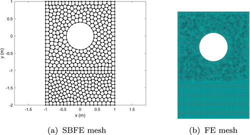
Consider a viscoelastic rectangular plate with a hole, which is composed of two kinds of materials in subdomains ${\mathrm{\Omega }}_1$ and ${\mathrm{\Omega }}_2$, and subjected to a uniform tension $p=1\mathrm{N}/{\mathrm{m}}^2$, as shown in Figure 3. The SBFE mesh consists of 500 polygon elements and 996 nodes, as shown in Figure 4(a).

Figure 3. Viscoelastic rectangular plate with a hole.

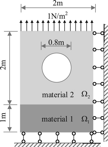
Figure 4. SBFE and FE meshes. (a) SBFE mesh and (b) FE mesh.

$({\tilde{E}}_1{)}_{{\mathrm{\Omega }}_1},({\tilde{E}}_2{)}_{{\mathrm{\Omega }}_1},({\tilde{\eta }}_1{)}_{{\mathrm{\Omega }}_1},(\tilde{v}{)}_{{\mathrm{\Omega }}_1}$ and $({\tilde{E}}_1{)}_{{\mathrm{\Omega }}_2},({\tilde{E}}_2{)}_{{\mathrm{\Omega }}_2},({\tilde{\eta }}_1{)}_{{\mathrm{\Omega }}_2},(\tilde{v}{)}_{{\mathrm{\Omega }}_2}$ are designated to denote the fuzzy viscoelastic constitutive parameters in ${\mathrm{\Omega }}_1$ and ${\mathrm{\Omega }}_2$, respectively. $(E_1{)}_{{\mathrm{\Omega }}_1},(E_2{)}_{{\mathrm{\Omega }}_1},({\eta }_1{)}_{{\mathrm{\Omega }}_1},(v{)}_{{\mathrm{\Omega }}_1}$ and $(E_1{)}_{{\mathrm{\Omega }}_2},(E_2{)}_{{\mathrm{\Omega }}_2},({\eta }_1{)}_{{\mathrm{\Omega }}_2},(v{)}_{{\mathrm{\Omega }}_2}$ refer to the deterministic viscoelastic constitutive parameters in ${\mathrm{\Omega }}_1$ and ${\mathrm{\Omega }}_2$, respectively.

Assume the values of membership functions of displacements are partially known spatially and temporally, and given by the solutions of forward fuzzy problems with the prescribed fuzzy viscoelastic constitutive parameters, the task of the fuzzy inverse problems is to seek the prescribed membership functions of fuzzy viscoelastic constitutive parameters using the above values.

Three cases are designed to examine the effectiveness of the proposed algorithm, and the impacts of temporal and spatial selections of measurement points on the identification results are taken into account.

5.1. Case 1: TPAA- and DSG-based solutions of the deterministic forward problem

Using the peak values given in Table 1, a comparison of the deterministic forward solutions obtained by TPAA-SBFEM with different time steps is shown in Figure 5, and the reference solution is given by a converged solution of ABAQUS (Figure 4(b),10034 quadratic quadrilateral elements and 30604 nodes, step size is $0.025\mathrm{s}$). With three groups of viscoelastic constitutive parameters randomly selected from the worst-case intervals [51] of Table 1, as shown in Table 2, a comparison of DSG and TPAA-SBFEM-based deterministic forward solutions is given in Figure 6.

Figure 5. Comparison of deterministic displacements in the y-direction with different step sizes (x = 1, y = 1).

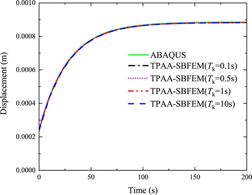
Figure 6. Comparison of deterministic displacements obtained from TPAA-SBFEM and DSG with different groups of constitutive parameters in the y-direction (x = 1, y = 1).

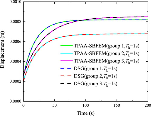
Table 1. Fuzzy viscoelastic constitutive parameters.

Fuzzy parameter	Peak value	Worst-case interval
$({\tilde{E}}_1{)}_{{\mathrm{\Omega }}_1}$ (Pa)	1.9600E+04	[1.1760E+04, 2.7440E+04]
$({\tilde{E}}_2{)}_{{\mathrm{\Omega }}_1}$ (Pa)	1.9600E+04	[1.1760E+04, 2.7440E+04]
$({\tilde{\eta }}_1{)}_{{\mathrm{\Omega }}_1}$ (Pa·s)	6.3542E+05	[3.8125E+05, 8.8959E+05]
$(\tilde{v}{)}_{{\mathrm{\Omega }}_1}$	2.3000E−01	[1.3800E−01, 3.2200E−01]
$({\tilde{E}}_1{)}_{{\mathrm{\Omega }}_2}$ (Pa)	1.9600E+03	[1.1760E+03, 2.7440E+03]
$({\tilde{E}}_2{)}_{{\mathrm{\Omega }}_2}$ (Pa)	9.8000E+03	[5.8800E+03, 1.3720E+04]
$({\tilde{\eta }}_1{)}_{{\mathrm{\Omega }}_2}$ (Pa·s)	5.2083E+04	[3.1250E+04, 7.2916E+04]
$(\tilde{v}{)}_{{\mathrm{\Omega }}_2}$	3.0000E−01	[1.8000E−01, 4.2000E−01]

Table 2. Groups of deterministic viscoelastic constitutive parameters.

Deterministic parameter	Group 1	Group 2	Group 3
$(E_1{)}_{{\mathrm{\Omega }}_1}$ (Pa)	2.4535E+04	2.6774E+04	1.8373E+04
$(E_2{)}_{{\mathrm{\Omega }}_1}$ (Pa)	2.5963E+04	2.6889E+04	2.6119E+04
$({\eta }_1{)}_{{\mathrm{\Omega }}_1}$ (Pa·s)	4.4580E+05	4.6137E+05	7.8396E+05
$(v{)}_{{\mathrm{\Omega }}_1}$	3.0606E−01	3.1659E−01	3.1455E−01
$(E_1{)}_{{\mathrm{\Omega }}_2}$ (Pa)	2.1675E+03	2.6768E+03	2.2042E+03
$(E_2{)}_{{\mathrm{\Omega }}_2}$ (Pa)	6.6447E+03	9.6853E+03	6.1600E+03
$({\eta }_1{)}_{{\mathrm{\Omega }}_2}$ (Pa·s)	4.2854E+04	6.4594E+04	6.6630E+04
$(v{)}_{{\mathrm{\Omega }}_2}$	3.1125E−01	2.1405E−01	4.0416E−01

5.2. Case 2: Identification of linear membership functions

Assume the membership functions of fuzzy viscoelastic constitutive parameters are linear with a triangular distribution [51], and their peak values and worst-case intervals [51] are given in Table 1.

All membership functions of fuzzy viscoelastic constitutive parameters are uniformly divided into 11 α-sublevels.

For the forward problem, a comparison of fuzzy displacements at a feature point is shown in Figure 7, in which the reference solution is given via $2\times {10}^7$ Monte Carlo simulations. The interval bounds of displacements at each of α-sublevels are compared when $t=200\mathrm{s}$, as shown in Table 3.

Figure 7. Comparison of fuzzy displacement in the y-direction for the linear membership functions (x = 1, y = 1). (a) DSGBE and (b) MCMBE.

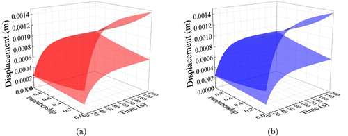
Table 3. Comparison of interval bounds of displacement for linear membership functions ($x=1,y=1$,$t=200\mathrm{s}$, y-direction).

	Lower bound			Upper bound
α-level	MCMBE (m)	DSGBE (m)	Relative error (%)	MCMBE (m)	DSGBE (m)	Relative error (%)
0.0	6.2520E−04	6.2023E−04	7.9493E−01	1.4657E−03	1.4789E−03	8.9994E−01
0.1	6.4452E−04	6.4003E−04	6.9749E−01	1.3657E−03	1.3860E−03	1.4898E+00
0.2	6.6693E−04	6.6064E−04	9.4319E−01	1.2864E−03	1.3042E−03	1.3812E+00
0.3	6.8813E−04	6.8271E−04	7.8759E−01	1.2166E−03	1.2314E−03	1.2188E+00
0.4	7.1041E−04	7.0604E−04	6.1532E−01	1.1546E−03	1.1663E−03	1.0112E+00
0.5	7.3447E−04	7.3079E−04	5.0166E−01	1.1006E−03	1.1072E−03	5.9729E−01
0.6	7.5978E−04	7.5710E−04	3.5307E−01	1.0490E−03	1.0532E−03	3.9688E−01
0.7	7.8718E−04	7.8526E−04	2.4410E−01	1.0011E−03	1.0049E−03	3.7934E−01
0.8	8.1676E−04	8.1562E−04	1.3957E−01	9.5814E−04	9.6042E−04	2.3894E−01
0.9	8.4857E−04	8.4780E−04	9.0970E−02	9.1914E−04	9.1988E−04	8.0993E−02

For the inverse problem, the measurement values are given by 20 displacements randomly selected from the forward fuzzy solutions. The identification results are shown in Figure 8, and the computational costs are compared in Table 4. Table 5 presents a comparison of the identification results at each of α-sublevels with different measurement points which are illustrated in Figure 11.

Figure 8. Comparison of the identification results for the linear membership functions.

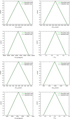
Table 4. Comparison of computational costs.

Task	Computational cost (s)
Construction of DSG in serial	1.5128E+05
Construction of DSG in parallel	9.5624E+03
Per deterministic solution using DSG	1.6396E−02
Per deterministic solution using TPAA-SBFEM	1.2718E+02
Serial identification of the worst-case intervals using DSG	2.7425E+04
Parallel identification of the worst-case intervals using DSG	1.6834E+03

Table 5. Maximum relative errors of identifications at each α-sublevel for linear membership functions.

	Maximum relative error
α-level	20 measured points	26 measured points	32 measured points	40 measured points
0.0	0.0002%	0.0001%	0.0001%	0.0000%
0.1	0.0530%	0.0590%	0.0490%	0.0353%
0.2	0.0001%	0.0002%	0.0001%	0.0001%
0.3	0.2683%	0.1569%	0.1682%	0.0341%
0.4	0.0002%	0.0076%	0.0068%	0.0040%
0.5	0.0001%	0.0014%	0.0015%	0.0015%
0.6	0.0003%	0.0000%	0.0001%	0.0087%
0.7	0.0002%	0.0001%	0.0001%	0.0000%
0.8	0.0001%	0.0002%	0.0001%	0.0000%
0.9	0.0002%	0.0000%	0.0000%	0.0000%
1.0	0.0000%	0.0001%	0.0000%	0.0000%

5.3. Case 3: Identification of nonlinear membership functions

Assume the membership functions of fuzzy viscoelastic constitutive parameters are quasi-Gaussian [52], and their peak values and worst-case intervals [51] are the same as Table 1.

All membership functions of the constitutive parameters are uniformly divided into 21 α-sublevels.

For the forward problem, a comparison of fuzzy displacements at a feature point is shown in Figure 9, in which the reference solution is given via $2\times {10}^7$ Monte Carlo simulations. The interval bounds of displacements at each of α-sublevels are compared when $t=200\mathrm{s}$, as shown in Table 6.

Figure 9. Comparison of fuzzy displacement in the y-direction for the nonlinear membership functions (x = 1, y = 1). (a) DSGBE and (b) MCMBE.

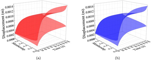
Table 6. Comparison of interval bounds of displacement for nonlinear membership functions (x = 1, y = 1, $t=200\mathrm{s}$, y-direction).

	Lower bound			Upper bound
α-level	MCMBE (m)	DSGBE (m)	Relative error (%)	MCMBE (m)	DSGBE (m)	Relative error (%)
0.00	6.2526E−04	6.2023E−04	8.0439E−01	1.4582E−03	1.4789E−03	1.4229E+00
0.05	6.6162E−04	6.5725E−04	6.6090E−01	1.2973E−03	1.3166E−03	1.4904E+00
0.10	6.8348E−04	6.7911E−04	6.3947E−01	1.2306E−03	1.2422E−03	9.4280E−01
0.15	6.9845E−04	6.9527E−04	4.5561E−01	1.1875E−03	1.1976E−03	8.5406E−01
0.20	7.1028E−04	7.0651E−04	5.3154E−01	1.1546E−03	1.1651E−03	9.1439E−01
0.25	7.2043E−04	7.1694E−04	4.8522E−01	1.1295E−03	1.1390E−03	8.4529E−01
0.30	7.3092E−04	7.2640E−04	6.1745E−01	1.1090E−03	1.1169E−03	7.1477E−01
0.35	7.3806E−04	7.3514E−04	3.9574E−01	1.0888E−03	1.0977E−03	8.2072E−01
0.40	7.4693E−04	7.4343E−04	4.6874E−01	1.0762E−03	1.0805E−03	4.0142E−01
0.45	7.5438E−04	7.5139E−04	3.9641E−01	1.0586E−03	1.0641E−03	5.2608E−01
0.50	7.6210E−04	7.5939E−04	3.5574E−01	1.0468E−03	1.0488E−03	1.9310E−01
0.55	7.7011E−04	7.6691E−04	4.1530E−01	1.0321E−03	1.0356E−03	3.4214E−01
0.60	7.7697E−04	7.7453E−04	3.1399E−01	1.0185E−03	1.0227E−03	4.1313E−01
0.65	7.8548E−04	7.8250E−04	3.7915E−01	1.0064E−03	1.0092E−03	2.7389E−01
0.70	7.9281E−04	7.9068E−04	2.6850E−01	9.9367E−04	9.9607E−04	2.4065E−01
0.75	8.0110E−04	7.9920E−04	2.3762E−01	9.8048E−04	9.8323E−04	2.8024E−01
0.80	8.1026E−04	8.0834E−04	2.3760E−01	9.6893E−04	9.7005E−04	1.1531E−01
0.85	8.2006E−04	8.1850E−04	1.9103E−01	9.5465E−04	9.5624E−04	1.6666E−01
0.90	8.3172E−04	8.3022E−04	1.8041E−01	9.3942E−04	9.4107E−04	1.7576E−01
0.95	8.4633E−04	8.4555E−04	9.2047E−02	9.2154E−04	9.2253E−04	1.0743E−01

For the inverse problem, the measurement values are given by 40 fuzzy displacements randomly selected from the forward fuzzy solutions. The identification results are shown in Figure 10. Table 7 exhibits the maximum errors of identifications with different temporal and spatial selections of measurement points, as illustrated in Figure 11.

Figure 10. Comparison of the identification results for the nonlinear membership functions.

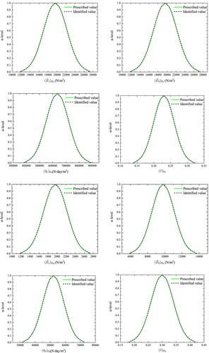
Figure 11. The distributions of measured points. (a) 20 measured points, (b) 26 measured points, (c) 32 measured points and (d) 40 measured points.

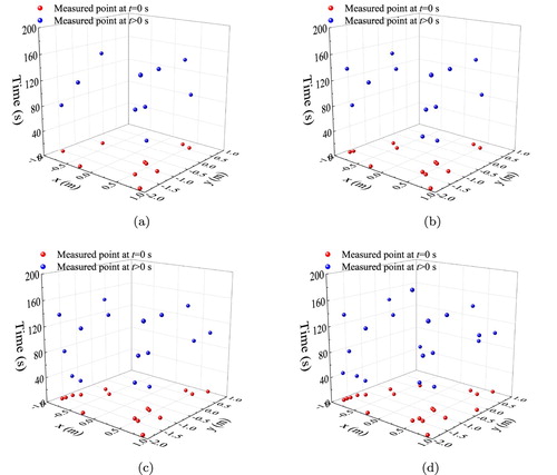
Table 7. Maximum relative errors of identifications at each α-sublevel for nonlinear membership functions.

	Maximum relative error
α-level	20 measured points	26 measured points	32 measured points	40 measured points
0.00	0.0001%	0.0001%	0.0000%	0.0001%
0.05	0.0001%	0.0001%	0.0001%	0.0001%
0.10	0.0471%	0.0457%	0.0481%	0.0223%
0.15	0.2187%	0.2026%	0.2310%	0.0685%
0.20	0.0001%	0.0083%	0.0056%	0.0047%
0.25	0.0004%	0.0076%	0.0064%	0.3384%
0.30	0.0001%	0.0040%	0.0035%	0.0020%
0.35	0.0001%	0.0001%	0.0001%	0.0001%
0.40	0.0003%	0.0001%	0.0001%	0.0003%
0.45	0.0001%	0.0001%	0.0001%	0.0140%
0.50	0.0000%	0.0001%	0.0000%	0.2924%
0.55	0.0001%	0.0001%	0.0002%	0.0017%
0.60	0.0001%	0.0000%	0.0002%	0.0010%
0.65	0.0001%	0.0001%	0.0000%	0.0000%
0.70	0.0001%	0.0002%	0.0000%	0.0000%
0.75	0.0001%	0.0002%	0.0000%	0.0001%
0.80	0.0002%	0.0002%	0.0001%	0.0001%
0.85	0.0001%	0.0001%	0.0000%	0.0000%
0.90	0.0002%	0.0005%	0.0001%	0.0000%
0.95	0.0002%	0.0001%	0.0000%	0.0001%
1.00	0.0000%	0.0000%	0.0000%	0.0000%

5.4. Remarks on the numerical examples

1. As shown in Figure 5, the deterministic forward solutions given by TPAA-SBFEM have good accordance with the ABAQUS solutions. A sufficient computing accuracy can be achieved via an adaptive procedure for different step sizes, even the step size increases a hundredfold.

2. DSG surrogate solutions are sufficiently accurate comparing with the TPAA-SBFEM solutions, as shown in Figure 6. The forward fuzzy solutions given by DSG-based bounds estimation (DSGBE) are well matched with the Monte Carlo method-based bounds estimation (MCMBE), as shown in Figure 7 for the case 2 and in Figure 9 for the case 3. For case 2, the maximum relative error of lower bound estimation at $t=200\mathrm{s}$ is 0.94% and is 1.49% for the upper bound estimation, as shown in Table 3. For case 3, the maximum relative error of the lower bound estimation at $t=200\mathrm{s}$ is 0.80% and is 1.49% for the upper bound estimation, as shown in Table 6.

3. The proposed algorithm is capable of identifying linear or nonlinear membership functions of viscoelastic constitutive parameters with sufficient accuracy, as shown in Figures 8 and 10. The maximum relative error of identification is 0.27% for case 2, as shown in Table 5 and is 0.34% for case 3, as shown in Table 7.

4. As shown in Table 4, the average computing time for a deterministic solution using DSG surrogate is considerably cheap than that using TPAA-SBFEM, and the computational cost of inverse fuzzy analysis can be effectively reduced by the surrogate and parallelization. Compared with the computing time of the serial construction of DSG, a 15.82 speedup can be gained via parallel construction. Using the paralleled particle swarm method, instead of the serial one, a 16.29 speedup can be gained in the identification of the worst-case intervals.

5. The identification results seem not sensitive to the temporal and spatial selections of measurement points, as shown in Table 5 for case 2 and in Table 7 for case 3.

6. Conclusions

By integrating the advantages of SBFEM and TPAA, the surrogate technique and optimization algorithm, an efficient numerical algorithm is presented to solve the inverse fuzzy viscoelastic problem of identification.

The major contributions of this paper include the following:

1. A two-stage strategy cooperating with the particle swarm method is presented to solve the inverse fuzzy problem of identification. At each stage, the inverse fuzzy problem is solved via a series of α-level strategy based inverse interval problems. Therefore, when there is a fuzzy uncertainty in the displacement measurement, the membership functions of viscoelastic constitutive parameters can be identified.

2. An α-level strategy and optimization technique-based algorithm is proposed for the forward fuzzy analysis required for solving inverse fuzzy problems, which is capable of providing membership functions of displacement when there is a fuzzy uncertainty in the viscoelastic constitutive parameters.

3. A DSG surrogate is constructed with high fidelity deterministic solutions provided by SBFEM and TPAA and is embedded in the optimization process of solving inverse interval problems to alleviate the heavy computational cost caused by repeated time-dependent deterministic solutions.

4. By virtue of a Parallel Computing Toolbox in MATLAB, the parallelization is realized for the construction of DSG surrogate and the implementation of the particle swarm method for a further reduction of computational expense.

5. Numerical verifications with the regional inhomogeneity are provided, and the impacts of temporal and spatial selections of measurement points on the identification results are taken into account.

Acknowledgements

The work presented in this paper has been supported by NSF (11572068), NSF (11972109), NKBRP (2015CB057804), Natural Science Funding of Liaoning Province (2020-MS-110), and the Fundamental Research Funds for the Central Universities (DUT20LK09).

Disclosure statement

No potential conflict of interest was reported by the author(s).

Additional information

Funding

This work was supported by the National Natural Science Foundation of China [11572068, 11972109], Major State Basic Research Development Program of China [2015CB057804], Fundamental Research Funds for the Central Universities [DUT20LK09] and Natural Science Funding of Liaoning Province [2020-MS-110].

Appendix. Calculation of stiffness matrix of a SBFEM element

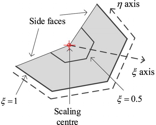
The SBFEM [40] introduces a normalized radial coordinate system by scaling the domain boundary relative to a scaling centre $O(x_0,y_0)$, as shown in Figure 1, the normalized radial coordinate ξ runs from the scaling centre towards the boundary, and has a value of zero at the scaling centre and unity at the boundary. The other circumferential coordinate η specifies a distance around the boundary from an origin on the boundary.

Figure A1. A scaled coordinate system.

The scaled boundary and Cartesian coordinate systems are related by the scaling equations (A1) $\begin{array}{rl}& x=x_0+\xi x_{\eta }(\eta ),\end{array}$(A1) (A2) $\begin{array}{rl}& y=y_0+\xi y_{\eta }(\eta ),\end{array}$(A2) where $(x_{\eta },y_{\eta })$ is a point on the line element.

The displacement at any point within an element is approximated as (A3) $u(\xi ,\eta )=\mathbf{N}(\eta )\mathbf{u}(\xi ),$(A3) where the unknown vector $\mathbf{u}(\xi )$ is a set of functions analytical in ξ. Only a boundary discretization is required in the SBFEM. The approximated stresses are in the form (A4) $\mathit{\sigma }(\xi ,\eta )=\mathbf{D}\mathit{\epsilon }(\xi ,\eta )=\mathbf{D}({\mathbf{B}}_1(\eta )\frac{\mathrm{\partial }\mathbf{u}(\xi )}{\mathrm{\partial }\xi }+\frac{1}{\xi }{\mathbf{B}}_2(\eta )\mathbf{u}(\xi )),$(A4) where (A5) $\begin{array}{rl}& {\mathbf{B}}_1(\eta )={\mathbf{b}}_1(\eta )\mathbf{N}(\eta ),\end{array}$(A5) (A6) $\begin{array}{rl}& {\mathbf{B}}_2(\eta )={\mathbf{b}}_2(\eta )\frac{\mathrm{\partial }\mathbf{N}(\eta )}{\mathrm{\partial }\eta }.\end{array}$(A6) ${\mathbf{b}}_1(\eta )$ and ${\mathbf{b}}_2(\eta )$ are dependent only on the boundary definition [40].

Utilizing the virtual displacement principle then gives (in the absence of body force) (A7) ${\int }_{\mathrm{\Omega }}\delta \mathit{\epsilon }(\xi ,\eta {)}^{\mathrm{T}}\mathit{\sigma }(\xi ,\eta )\mathrm{d}\mathrm{\Omega }={\int }_{\eta }\delta \mathbf{u}(\eta {)}^{\mathrm{T}}\mathbf{p}(\eta )\mathrm{d}\eta .$(A7) Substituting Equation (A4(A4) $\mathit{\sigma }(\xi ,\eta )=\mathbf{D}\mathit{\epsilon }(\xi ,\eta )=\mathbf{D}({\mathbf{B}}_1(\eta )\frac{\mathrm{\partial }\mathbf{u}(\xi )}{\mathrm{\partial }\xi }+\frac{1}{\xi }{\mathbf{B}}_2(\eta )\mathbf{u}(\xi )),$(A4) ) into Equation (A7(A7) ${\int }_{\mathrm{\Omega }}\delta \mathit{\epsilon }(\xi ,\eta {)}^{\mathrm{T}}\mathit{\sigma }(\xi ,\eta )\mathrm{d}\mathrm{\Omega }={\int }_{\eta }\delta \mathbf{u}(\eta {)}^{\mathrm{T}}\mathbf{p}(\eta )\mathrm{d}\eta .$(A7) ), and integrating the area integrals containing $\mathrm{\partial }\delta \mathbf{u}(\xi )/\mathrm{\partial }\xi$ with respect to ξ using Green's Theorem, (A8) $\begin{array}{rl}& {\int }_{\mathrm{\Omega }}\delta \mathit{\epsilon }(\xi ,\eta {)}^{\mathrm{T}}\mathbf{D}\mathit{\epsilon }(\xi ,\eta )\mathrm{d}V\\ & =\delta \mathbf{u}(\xi {)}^{\mathrm{T}}({\mathbf{E}}^0{\displaystyle \frac{\mathrm{\partial }\mathbf{u}(\xi )}{\mathrm{\partial }\xi }}+({\mathbf{E}}^1{)}^{\mathrm{T}}\mathbf{u}(\xi ))\\ & -{\int }_0^1\delta \mathbf{u}(\xi {)}^{\mathrm{T}}\{{\mathbf{E}}^0\xi \frac{{\mathrm{\partial }}^2\mathbf{u}(\xi )}{\mathrm{\partial }{\xi }^2}+({\mathbf{E}}^0+({\mathbf{E}}^1{)}^{\mathrm{T}}-{\mathbf{E}}^1)\frac{\mathrm{\partial }\mathbf{u}(\xi )}{\mathrm{\partial }\xi }-{\mathbf{E}}^2\frac{1}{\xi }\mathbf{u}(\xi )\}\mathrm{d}\xi \\ & =\delta \mathbf{u}(\xi {)}^{\mathrm{T}}\mathbf{P},\end{array}$(A8) where (A9) $\begin{array}{rl}& {\mathbf{E}}^0={\int }_{\eta }({\mathbf{B}}_1(\eta ){)}^{\mathrm{T}}\mathbf{D}{\mathbf{B}}_1(\eta )|\mathbf{J}|\mathrm{d}\eta ,\end{array}$(A9) (A10) $\begin{array}{rl}& {\mathbf{E}}^1={\int }_{\eta }({\mathbf{B}}_2(\eta ){)}^{\mathrm{T}}\mathbf{D}{\mathbf{B}}_1(\eta )|\mathbf{J}|\mathrm{d}\eta ,\end{array}$(A10) (A11) $\begin{array}{rl}& {\mathbf{E}}^2={\int }_{\eta }({\mathbf{B}}_2(\eta ){)}^{\mathrm{T}}\mathbf{D}{\mathbf{B}}_2(\eta )|\mathbf{J}|\mathrm{d}\eta .\end{array}$(A11) $|\mathbf{J}\mathbf{|}$ is the Jacobian at the boundary $(\xi =1)$. $\mathbf{P}$ denotes the vector of equivalent nodal forces.

The arbitrariness of $\delta \mathbf{u}(\xi )$ results in (A12) $\begin{array}{rl}& \mathbf{P}={\mathbf{E}}^0\frac{\mathrm{\partial }\mathbf{u}(\xi )}{\mathrm{\partial }\xi }+({\mathbf{E}}^1{)}^{\mathrm{T}}\mathbf{u}(\xi ),\end{array}$(A12) (A13) $\begin{array}{rl}& {\mathbf{E}}^0{\xi }^2\frac{{\mathrm{\partial }}^2\mathbf{u}(\xi )}{\mathrm{\partial }{\xi }^2}+({\mathbf{E}}^0+({\mathbf{E}}^1{)}^{\mathrm{T}}-{\mathbf{E}}^1)\xi \frac{\mathrm{\partial }\mathbf{u}(\xi )}{\mathrm{\partial }\xi }-{\mathbf{E}}^2\mathbf{u}(\xi )=\mathbf{0.}\end{array}$(A13) By inspection, the solutions to the homogeneous set of Euler–Cauchy differential equations represented by Equation (A13(A13) $\begin{array}{rl}& {\mathbf{E}}^0{\xi }^2\frac{{\mathrm{\partial }}^2\mathbf{u}(\xi )}{\mathrm{\partial }{\xi }^2}+({\mathbf{E}}^0+({\mathbf{E}}^1{)}^{\mathrm{T}}-{\mathbf{E}}^1)\xi \frac{\mathrm{\partial }\mathbf{u}(\xi )}{\mathrm{\partial }\xi }-{\mathbf{E}}^2\mathbf{u}(\xi )=\mathbf{0.}\end{array}$(A13) ) must be of the form [40] (A14) $\mathbf{u}(\xi )=c_1{\xi }^{-1}{\mathit{\varphi }}_1+c_2{\xi }^{-{\lambda }_2}{\mathit{\varphi }}_2+\cdots ,$(A14) where the exponents $-{\lambda }_i$ and corresponding vectors ${\mathit{\varphi }}_{\mathit{i}}$ are independent modes of deformation in the ξ direction and $c_i$ is the integration constant for the contribution of each mode to the solution. Therefore, the displacement of each mode takes the form [40] (A15) $\mathbf{u}(\xi )={\xi }^{-\lambda }\mathit{\varphi },$(A15) where $\mathit{\varphi }$ refers to the vector of modal displacements at boundary nodes. λ is a modal scaling factor for the radial direction.

By submitting Equation (A15(A15) $\mathbf{u}(\xi )={\xi }^{-\lambda }\mathit{\varphi },$(A15) ), the solution of Equations (A12(A12) $\begin{array}{rl}& \mathbf{P}={\mathbf{E}}^0\frac{\mathrm{\partial }\mathbf{u}(\xi )}{\mathrm{\partial }\xi }+({\mathbf{E}}^1{)}^{\mathrm{T}}\mathbf{u}(\xi ),\end{array}$(A12) ) and (A13(A13) $\begin{array}{rl}& {\mathbf{E}}^0{\xi }^2\frac{{\mathrm{\partial }}^2\mathbf{u}(\xi )}{\mathrm{\partial }{\xi }^2}+({\mathbf{E}}^0+({\mathbf{E}}^1{)}^{\mathrm{T}}-{\mathbf{E}}^1)\xi \frac{\mathrm{\partial }\mathbf{u}(\xi )}{\mathrm{\partial }\xi }-{\mathbf{E}}^2\mathbf{u}(\xi )=\mathbf{0.}\end{array}$(A13) ) can be transferred into an eigenvalue problem defined by [40] (A16) $\left[\begin{array}{cc}({\mathbf{E}}^0{)}^{-1}({\mathbf{E}}^1{)}^{\mathrm{T}}& -({\mathbf{E}}^0{)}^{-1}\\ {\mathbf{E}}^1({\mathbf{E}}^0{)}^{-1}({\mathbf{E}}^1{)}^{\mathrm{T}}-{\mathbf{E}}^2& -{\mathbf{E}}^1({\mathbf{E}}^0{)}^{-1}\end{array}\right]\left\{\begin{array}{l}\mathit{\varphi }\\ \mathbf{q}\end{array}\right\}=\lambda \left\{\begin{array}{l}\mathit{\varphi }\\ \mathbf{q}\end{array}\right\},$(A16) where $\mathbf{q}$ refers to the vector of modal forces at boundary nodes. The solution of this standard eigenproblem yields $2n^{\ast }$ modes ($n^{\ast }$ is the number of DOFs of the system). The subset of $n^{\ast }$ modal displacements is designated by ${\mathbf{\Phi }}_1$, and the subset of modal forces corresponding to the $n^{\ast }$ modes in ${\mathbf{\Phi }}_1$ is denoted as ${\mathbf{Q}}_1$.

The integration constants $\mathbf{c}$ in Equation (A14(A14) $\mathbf{u}(\xi )=c_1{\xi }^{-1}{\mathit{\varphi }}_1+c_2{\xi }^{-{\lambda }_2}{\mathit{\varphi }}_2+\cdots ,$(A14) ) on the boundary $\xi =1$ are [40] (A17) $\mathbf{c}=({\mathbf{\Phi }}_1{)}^{-1}\mathbf{u}.$(A17) The equivalent nodal forces required to cause these displacements are [40] (A18) $\mathbf{P}={\mathbf{Q}}_1\mathbf{c}={\mathbf{Q}}_1({\mathbf{\Phi }}_1{)}^{-1}\mathbf{u}.$(A18) Thus, we have the element stiffness matrix [40] (A19) ${\mathbf{K}}_e={\mathbf{Q}}_1({\mathbf{\Phi }}_1{)}^{-1}.$(A19)

References

- Castello DA, Rochinha FA, Roitman N, Constitutive parameter estimation of a viscoelastic model with internal variables. Mech Syst Signal Process. 2008;22(8):1840–1857.
- Jager A, Lackner R, Eberhardsteiner J. Identification of viscoelastic properties by means of nanoindentation taking the real tip geometry into account. Meccanica. 2007;42(3):293–306.
- Leo CJ. Identification of a general poro-viscoelastic model of one-dimensional. In Proceedings of the Fourth International Conference on Soft Soil Engineering. Vancouver: CRC Press; 2006. p. 397.
- Lewandowski R, Chorazyczewski B. Identification of the parameters of the Kelvin-Voigt and the Maxwell fractional models, used to modeling of viscoelastic dampers. Comput Struct. 2010;88(1–2):1–17.
- Sarron JC, Blondeau C, Guillaume A, et al. Identification of linear viscoelastic constitutive models. J Biomech. 2000;33(6):685–693.
- Smilauer V, Bazant ZP. Identification of viscoelastic c-s-h behavior in mature cement paste by fft-based homogenization method. Cement Concrete Res. 2010;40(2):197–207.
- Tian YC, Zhang ZM, Wei PJ. Parametric inversion of viscoelastic media with homotopy method. Chin J Rock Mech Eng. 2006;25:1718–1722.
- Venture G, Yamane K, Nakamura Y, et al. Identification of human limb viscoelasticity using robotics methods to support the diagnosis of neuromuscular diseases. Int J Rob Res. 2009;28(10):1322–1333.
- Erdogan YS, Bakir PG. Inverse propagation of uncertainties in finite element model updating through use of fuzzy arithmetic. Eng Appl Artif Intell. 2013;26(1):357–367.
- Moens D, Hanss M. Non-probabilistic finite element analysis for parametric uncertainty treatment in applied mechanics: recent advances. Finite Elem Anal Des. 2011;47(1):4–16.
- Moens D, Vandepitte D. Recent advances in non-probabilistic approaches for non-deterministic dynamic finite element analysis. Arch Comput Methods Eng. 2006;13(3):389–464.
- Walz NP, Hanss M. Fuzzy arithmetical analysis of multibody systems with uncertainties. Arch Mech Eng. 2013;60(1):109–125.
- Wang C, Matthies HG, Qiu Z. Optimization-based inverse analysis for membership function identification in fuzzy steady-state heat transfer problem. Struct Multidiscipl Optim. 2017;57(4):1495–1505.
- Hernandez WP, Borges FCL, Castello DA, et al. Bayesian inference applied on model calibration of fractional derivative viscoelastic model. In V Steffen Jr, DA Rade, WM Bessa (Eds.), DINAME 2015-Proceedings of the XVII International Symposium on Dynamic Problems of Mechanics. Natal; 2015.
- Zhang E, Chazot J, Antoni J, et al. Bayesian characterization of Young's modulus of viscoelastic materials in laminated structures. J Sound Vib. 2013;332(16):3654–3666.
- Dosso SE, Holland CW. Geoacoustic uncertainties from viscoelastic inversion of seabed reflection data. IEEE J Ocean. Eng. 2006;31(3):657–671.
- Oates WS, Hays M, Miles P, et al. Uncertainty quantification and stochastic-based viscoelastic modeling of finite deformation elastomers. In Electroactive Polymer Actuators and Devices (EAPAD), vol. 8687. San Diego: SPIE; 2013. p. 86871O.
- Elishakoff I. Possible limitations of probabilistic methods in engineering. Appl Mech Rev. 2000;53(2):19.
- Moens D, Vandepitte D. A survey of non-probabilistic uncertainty treatment in finite element analysis. Comput Methods Appl Mech Eng. 2005;194(12–16):1527–1555.
- Santoro R, Muscolino G, Elishakoff I. Optimization and anti-optimization solution of combined parameterized and improved interval analyses for structures with uncertainties. Comput Struct. 2015;149:31–42.
- Wang C. Evidence-theory-based uncertain parameter identification method for mechanical systems with imprecise information. Comput Methods Appl Mech Eng. 2019;351:281–296.
- Liu J, Cao L, Jiang C, et al. Parallelotope-formed evidence theory model for quantifying uncertainties with correlation. Appl Math Model. 2020;77:32–48.
- Cao LX, Liu J, Jiang C, et al. Evidence-based structural uncertainty quantification by dimension reduction decomposition and marginal interval analysis. J Mech Design. 2020;142(5):051701-1–051701-12.
- Wang C, Matthies HG. Novel interval theory-based parameter identification method for engineering heat transfer systems with epistemic uncertainty. Int J Numer Methods Eng. 2018;115(6):756–770.
- Wang L, Liu Y, Liu Y. An inverse method for distributed dynamic load identification of structures with interval uncertainties. Adv Eng Softw. 2019;131:77–89.
- Wang L, Xiong C, Wang X, et al. Sequential optimization and fuzzy reliability analysis for multidisciplinary systems. Struct Multidiscip Optim. 2019;60:1079–1095.
- Wang L, Xiong C, Yang Y. A novel methodology of reliability-based multidisciplinary design optimization under hybrid interval and fuzzy uncertainties. Comput Methods Appl Mech Eng. 2018;337:439–457.
- Faes M, Moens D. Recent trends in the modeling and quantification of non-probabilistic uncertainty. Arch Comput Methods Eng. 2019;27:633–671.
- Haag T, Gonzalez SC, Hanss M. Model validation and selection based on inverse fuzzy arithmetic. Mech Syst Signal Process. 2012;32:116–134.
- Hanss M, Oexl S, Gaul L. Identification of a bolted-joint model with fuzzy parameters loaded normal to the contact interface. Mech Res Commun. 2002;29(2–3):177–187.
- Adhikari S, Khodaparast HH. A spectral approach for fuzzy uncertainty propagation in finite element analysis. Fuzzy Sets Syst. 2014;243:1–24.
- Mendes M, Ray S, Pereira JCF, et al. Quantification of uncertainty propagation due to input parameters for simple heat transfer problems. Int J Therm Sci. 2012;60:94–105.
- Sofi A, Muscolino G. Static analysis of Euler–Bernoulli beams with interval Young's modulus. Comput Struct. 2015;156:72–82.
- Yang HT, Li YX, Xue YN. Interval uncertainty analysis of elastic bimodular truss structures. Inverse Probl Sci Eng. 2015;23(4):578–589.
- Kennedy J, Eberhart R. Particle swarm optimization. In proceedings of ICNN'95-International Conference on Neural Networks, vol. 4. Perth: IEEE; 1995. p. 1942–1948.
- Mezura-Montes E, Coello C. Constraint-handling in nature-inspired numerical optimization: past, present and future. Swarm Evol Comput. 2011;1(4):173–194.
- Pedersen H, Erik M. Good parameters for particle swarm optimization. Denmark: Hvass Lab., Copenhagen; 2010. p. 1551–3203. (Tech. Rep. HL1001).
- Klimke A, Wohlmuth B. Computing expensive multivariate functions of fuzzy numbers using sparse grids. Fuzzy Sets Syst. 2005;154(3):432–453.
- Klimke A. Uncertainty modeling using fuzzy arithmetic and sparse grids [dissertation]. Stuttgart: Universität Stuttgart; 2006.
- Deeks AJ, Wolf JP. A virtual work derivation of the scaled boundary finite-element method for elastostatics. Comput Mech. 2002;28(6):489–504.
- He YQ, Yang HT. Solving viscoelastic problems by combining SBFEM and a temporally piecewise adaptive algorithm. Mech Time-Depend Mater. 2017;21(3):481–497.
- Yang HT. A new approach of time stepping for solving transfer problems. Commun Numer Methods Eng. 1999;15(5):325–334.
- Li SY. Engineering fuzzy mathematics with applications. Harbin: Harbin Institute of Technology Press; 2004. p. 5–30.
- Zienkiewicz OC, Taylor RL, Zhu JZ. The finite element method: its basis and fundamentals. Oxford: Butterworth-Heinemann; 2013.
- Shames IH, Cozzarelli FA. Elastic and inelastic stress analysis. Boca Raton: CRC Press; 1997.
- Wang C, He YQ, Yang HT. A SBFEM and sensitivity analysis based algorithm for solving inverse viscoelastic problems. Eng Anal Bound Elem. 2019;106:588–598.
- Klimke A, Wohlmuth B. Algorithm 847: spinterp: piecewise multilinear hierarchical sparse grid interpolation in MATLAB. ACM Trans Math Softw. 2005;31(4):561–579.
- Clenshaw CW, Curtis AR. A method for numerical integration on an automatic computer. Numer Math. 1960;2(1):197–205.
- Klimke A, Nunes RF, Wohlmuth BI. Fuzzy arithmetic based on dimension-adaptive sparse grids: a case study of a large-scale finite element model under uncertain parameters. Int J Uncertain Fuzziness Knowl-Based Syst. 2006;14(5):561–577.
- Hanss M. Applied fuzzy arithmetic. Berlin Heidelberg: Springer-Verlag; 2005.
- Hanss M. The extended transformation method for the simulation and analysis of fuzzy-parameterized models. Int J Uncertain Fuzziness Knowl-Based Syst. 2003;11(6):711–727.
- Hanss M. The transformation method for the simulation and analysis of systems with uncertain parameters. Fuzzy Sets Syst. 2002;130(3):277–289.
- Wu D, Gao W, Wang C, et al. Robust fuzzy structural safety assessment using mathematical programming approach. Fuzzy Sets Syst. 2016;293:30–49.