A homogenization function technique to solve the 3D inverse Cauchy problem of elliptic type equations in a closed walled shell

Abstract

We solve the inverse Cauchy problem of elliptic type partial differential equations in an arbitrary 3D closed walled shell for recovering unknown data on an inner surface, with the over-specified Cauchy boundary conditions given on an outer surface. We first derive a homogenization function in the 3D domain to annihilate the Dirichlet as well as the Neumann data on the outer surface. Then, we can transform the inverse Cauchy problem to solve a direct problem inside the closed walled shell, using the homogenization technique and the domain type collocation method. The boundary functions are constructed from the 3D Pascal polynomials multiplied by an elementary boundary function, which are adopted as the bases to expand the numerical solution of the transformed elliptic equation. A simple scaling regularization is employed to reduce the condition number of the linear system to determine the expansion coefficients. Several numerical examples are presented to show that the novel method can overcome the highly ill-posed property of the inverse Cauchy problem in the 3D closed walled shell. The proposed algorithm is robust against large noise up to $20\mathrm{\%}$ and very time saving to obtain accurate solution.

Keywords:

• 3D inverse Cauchy problem
• elliptic type equations
• homogenization function
• boundary functions
• domain type collocation method

2010 Mathematics Subject Classifications:

• Elliptic equations and systems
• Partialdifferential equations
• boundary value problems
• Computing methodologies andapplications
• Inverse problems

1. Introduction

The present numerical solution of the 3D inverse Cauchy problem is to solve an under-specified boundary value problem of an elliptic type partial differential equation (PDE) in a closed walled shell, with the Cauchy data over-specified on an accessible outer boundary. For the purpose of the completion of data, one needs to recover the unknown data on an inaccessible inner boundary of the closed walled shell. However, the inverse Cauchy problem of the elliptic type PDEs is a difficult issue, since the solution does not depend continuously on the given Cauchy data. The errors in the given data may be extremely amplified in the numerical solution, if we cannot get rid of the ill-posedness of the inverse Cauchy problem.

For example, it is ill-posed for the inverse Cauchy problem of the Laplace equation: $\frac{{\mathrm{\partial }}^{2}u}{\mathrm{\partial }{x}^2}+\frac{{\mathrm{\partial }}^{2}u}{\mathrm{\partial }{y}^2}=0,$ together with the one-side Cauchy boundary conditions: (1) $\begin{array}{rl}& u(x,0)=h(x)=0,\end{array}$(1) (2) $\begin{array}{rl}& \frac{\mathrm{\partial }u}{\mathrm{\partial }y}(x,0)=g(x)=n^{-1}\sin (nx),\end{array}$(2) because the solution $u(x,y)=n^{-2}\sin (nx)\sinh (ny)$ does not tend to zero for any nonzero y, even the boundary condition $g(x)=n^{-1}\sin (nx)$ tends to zero by increasing n. It is apparent that the solution does not depend continuously on the boundary data $g(x)$. Hence, the inverse Cauchy problem is not well-posed in the sense of Hadamard.

The inverse Cauchy problem is not a fictitious problem without having physical application. The Cauchy boundary conditions (1(1) $\begin{array}{rl}& u(x,0)=h(x)=0,\end{array}$(1) ) and (2(2) $\begin{array}{rl}& \frac{\mathrm{\partial }u}{\mathrm{\partial }y}(x,0)=g(x)=n^{-1}\sin (nx),\end{array}$(2) ) are often encountered in the non-destructive testing of solid materials. As an example, the electrostatic image used in the non-destructive testing of metallic plates leads to such an inverse Cauchy problem for the Laplace equation in a two-dimensional domain. In order to detect the unknown shape of the inclusion within a conducting metal, the over-determined Cauchy data (the voltage and current) are imposed on the accessible exterior boundary. This amounts to solving an inverse Cauchy problem from the available Cauchy boundary data on the outer boundary.

In the past few decades, the inverse Cauchy problems of elliptic type equations have been studied extensively. Because they are highly ill-posed in nature [1], the inverse Cauchy problems have been solved by using different numerical methods [2–20]. There are two types of approaches to solve the inverse Cauchy problems. When the first type methods bring the ill-posed problems into a class of well-posed problems in the Tikhonov's sense [21–23], the second type methods are using iteration techniques [24–32]. The most existent numerical methods only consider the inverse Cauchy problems in two-dimensional domains, including the Laplace equation, the Poisson equation, the Helmholtz equation, and the modified Helmholtz equation, etc. Up to now, there are rare papers to solve the inverse Cauchy problems of three-dimensional elliptic type equations in three-dimensional domains [2,33–40].

In the paper, the proposed method will be used to solve the inverse Cauchy problem in an arbitrary 3D closed walled shell. Instead of the Tikhonov type regularization methods and the iterative methods, as an alternative one, we approach the numerical method based on a novel scheme, by directly collocating points inside the closed walled shell to satisfy the transformed elliptic equation to find the numerical solution of the new variable, which rendering the original variable automatically satisfies the over-specified Cauchy boundary conditions on the outer surface of the three-dimensional closed walled shell.

The other portions of the paper are arranged as follows. In Section 2, we specify the inverse Cauchy problem of a general elliptic type linear PDE in a closed walled shell. In Section 3, we derive a homogenization function, which annihilates the over-specified Cauchy data on the outer boundary. Then, a homogenization technique, elementary boundary function and higher-order boundary functions are constructed in Section 4, where we express the new variable in terms of the boundary functions as the bases of numerical solution, which satisfies the homogeneous Cauchy boundary conditions on the outer boundary automatically. Several numerical examples are given in Section 5, to assess the performance of the new method in the solutions of the inverse Cauchy problems in the closed walled shells. Finally, the conclusions are drawn in Section 6.

2. The inverse Cauchy problem in a closed walled shell

We consider the following inverse Cauchy problem of a general elliptic type linear PDE in a closed walled shell: (3) $\begin{array}{rl}& \mathrm{\Delta }u=f(\mathbf{x},u,\mathrm{\nabla }u),\mathbf{x}\in \mathrm{\Omega }\subset {\mathbb{R}}^3,\end{array}$(3) (4) $\begin{array}{rl}& u{|}_{\mathbf{x}\in {\mathrm{\Gamma }}_o}=h(\mathbf{x}),\end{array}$(4) (5) $\begin{array}{rl}& \mathrm{\nabla }u(\mathbf{x})\cdot \mathbf{n}{|}_{\mathbf{x}\in {\mathrm{\Gamma }}_o}=g(\mathbf{x}),\end{array}$(5) where Δ is the three-dimensional Laplacian operator and f is a linear function of $(u,\mathrm{\nabla }u)$, in which $\mathrm{\nabla }u$ is a gradient operator acting on u and ${\mathrm{\Gamma }}_o$ is the outer surface of the closed walled shell as shown in Figure 1. More specifically, the elliptic linear PDE we consider is (6) $\frac{{\mathrm{\partial }}^{2}u}{\mathrm{\partial }{x}^2}+\frac{{\mathrm{\partial }}^{2}u}{\mathrm{\partial }{y}^2}+\frac{{\mathrm{\partial }}^{2}u}{\mathrm{\partial }{z}^2}+a(\mathbf{x})\frac{\mathrm{\partial }u}{\mathrm{\partial }x}+b(\mathbf{x})\frac{\mathrm{\partial }u}{\mathrm{\partial }y}+c(\mathbf{x})\frac{\mathrm{\partial }u}{\mathrm{\partial }z}+d(\mathbf{x})u=S(x,y,z),$(6) where the coefficients are functions of $\mathbf{x}:=(x,y,z)$ and $S(x,y,z)$ is the given source function.

Figure 1. A schematic plot of 3D inverse Cauchy problem in a closed walled shell.

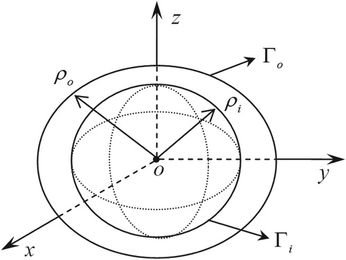
It is convenient to consider the inverse Cauchy problem in the spherical coordinates $(r,\theta ,\varphi )$, whose relations to the Cartesian coordinates $\mathbf{x}:=(x,y,z{)}^T$ are (7) $\begin{array}{l}x=r\cos \theta \sin \varphi ,\\ y=r\sin \theta \sin \varphi ,\\ z=r\cos \varphi ,\end{array}r\in [{\rho }_i,{\rho }_o],\theta \in [0,2\pi ],\varphi \in [0,\pi ],$(7) where $r=\sqrt{x^2+y^2+z^2}$, ${\rho }_i$ is the inner radius function and ${\rho }_o$ is the outer radius function of the closed walled shell, whose domain is denoted by $\mathrm{\Omega }=\{(x,y,z)|0<{\rho }_i(\theta ,\varphi )<r<{\rho }_o(\theta ,\varphi )\}$, with ${\mathrm{\Gamma }}_o=\{(x,y,z)|r={\rho }_o(\theta ,\varphi )\}$ being the outer surface, and with ${\mathrm{\Gamma }}_i=\{(x,y,z)|r={\rho }_i(\theta ,\varphi )\}$ being the inner surface. The point $(x,y,z)\in \mathrm{\Omega }$ is located between the inner surface ${\mathrm{\Gamma }}_i$ and the outer surface ${\mathrm{\Gamma }}_o$, with ${\rho }_i<r<{\rho }_o$. A schematic representation of the 3D inverse Cauchy problem in a closed walled shell is shown in Figure 1. We must emphasize that ${\rho }_o$ and ${\rho }_i$ are not necessarily constant, which are functions of $(\theta ,\varphi )$.

We impose the over-specified Cauchy boundary conditions (4(4) $\begin{array}{rl}& u{|}_{\mathbf{x}\in {\mathrm{\Gamma }}_o}=h(\mathbf{x}),\end{array}$(4) ) and (5(5) $\begin{array}{rl}& \mathrm{\nabla }u(\mathbf{x})\cdot \mathbf{n}{|}_{\mathbf{x}\in {\mathrm{\Gamma }}_o}=g(\mathbf{x}),\end{array}$(5) ) on ${\mathrm{\Gamma }}_o$. The present inverse Cauchy problem in the closed walled shell is to recover the unknown boundary data on ${\mathrm{\Gamma }}_i$ under the Cauchy data $h(\mathbf{x})$ and $g(\mathbf{x})$ over-specified on ${\mathrm{\Gamma }}_o$.

Instead of $u(x,y,z)$, we may write (8) $u(r,\theta ,\varphi ):=u(x=r\cos \theta \sin \varphi ,y=r\sin \theta \sin \varphi ,z=r\cos \varphi ),$(8) and the gradient of $u(r,\theta ,\varphi )$ in the spherical coordinates reads as (9) $\mathrm{\nabla }u=\frac{\mathrm{\partial }u}{\mathrm{\partial }r}{\mathbf{e}}_r+\frac{1}{r\sin \varphi }\frac{\mathrm{\partial }u}{\mathrm{\partial }\theta }{\mathbf{e}}_{\theta }+\frac{1}{r}\frac{\mathrm{\partial }u}{\mathrm{\partial }\varphi }{\mathbf{e}}_{\varphi },$(9) where ${\mathbf{e}}_r$, ${\mathbf{e}}_{\theta }$ and ${\mathbf{e}}_{\varphi }$ are, respectively, the unit vectors in the r, θ and φ directions.

When the symbol Δ denotes the Laplacian operator in the spherical coordinates, it is written as (10) $\mathrm{\Delta }u=\frac{{\mathrm{\partial }}^{2}u}{\mathrm{\partial }{r}^2}+\frac{2}{r}\frac{\mathrm{\partial }u}{\mathrm{\partial }r}+\frac{1}{r^2{\sin }^2\varphi }\frac{{\mathrm{\partial }}^{2}u}{\mathrm{\partial }{\theta }^2}+\frac{1}{r^2}\frac{{\mathrm{\partial }}^{2}u}{\mathrm{\partial }{\varphi }^2}+\frac{\cos \varphi }{r^2\sin \varphi }\frac{\mathrm{\partial }u}{\mathrm{\partial }\varphi }.$(10) In terms of the spherical coordinates, the algebraic equation to describe the outer surface ${\mathrm{\Gamma }}_o$ is given by (11) $G(r,\theta ,\varphi ):=r-{\rho }_o(\theta ,\varphi )=0.$(11) Accordingly, the normal direction $\mathbf{n}$ on the outer surface ${\mathrm{\Gamma }}_o$ can be computed from (12) $\mathbf{n}:={\frac{\mathrm{\nabla }G}{\Vert \mathrm{\nabla }G\Vert }|}_{r={\rho }_o},$(12) where, (13) $\begin{array}{rl}& \mathrm{\nabla }G={\mathbf{e}}_r-\frac{1}{r\sin \varphi }{\rho }_{o,\theta }{\mathbf{e}}_{\theta }-\frac{1}{r}{\rho }_{o,\varphi }{\mathbf{e}}_{\varphi },\end{array}$(13) (14) $\begin{array}{rl}& \Vert \mathrm{\nabla }G\Vert =\sqrt{1+\frac{1}{r^2{\sin }^2\varphi }{\rho }_{o,\theta }^2+\frac{1}{r^2}{\rho }_{o,\varphi }^2},\end{array}$(14) with the aid of Equations (9(9) $\mathrm{\nabla }u=\frac{\mathrm{\partial }u}{\mathrm{\partial }r}{\mathbf{e}}_r+\frac{1}{r\sin \varphi }\frac{\mathrm{\partial }u}{\mathrm{\partial }\theta }{\mathbf{e}}_{\theta }+\frac{1}{r}\frac{\mathrm{\partial }u}{\mathrm{\partial }\varphi }{\mathbf{e}}_{\varphi },$(9) ) and (11(11) $G(r,\theta ,\varphi ):=r-{\rho }_o(\theta ,\varphi )=0.$(11) ). Throughout this paper, ${\rho }_{o,\theta }$ and ${\rho }_{o,\varphi }$ denote the partial derivatives of ${\rho }_o(\theta ,\varphi )$ with respect to θ and φ, respectively.

Inserting Equations (13(13) $\begin{array}{rl}& \mathrm{\nabla }G={\mathbf{e}}_r-\frac{1}{r\sin \varphi }{\rho }_{o,\theta }{\mathbf{e}}_{\theta }-\frac{1}{r}{\rho }_{o,\varphi }{\mathbf{e}}_{\varphi },\end{array}$(13) ) and (14(14) $\begin{array}{rl}& \Vert \mathrm{\nabla }G\Vert =\sqrt{1+\frac{1}{r^2{\sin }^2\varphi }{\rho }_{o,\theta }^2+\frac{1}{r^2}{\rho }_{o,\varphi }^2},\end{array}$(14) ) into Equation (12(12) $\mathbf{n}:={\frac{\mathrm{\nabla }G}{\Vert \mathrm{\nabla }G\Vert }|}_{r={\rho }_o},$(12) ) and taking $r={\rho }_o(\theta ,\varphi )$ on the outer surface ${\mathrm{\Gamma }}_o$, we can derive (15) $\mathbf{n}=\eta [{\mathbf{e}}_r-\frac{{\rho }_{o,\theta }}{{\rho }_o\sin \varphi }{\mathbf{e}}_{\theta }-\frac{{\rho }_{o,\varphi }}{{\rho }_o}{\mathbf{e}}_{\varphi }],$(15) where (16) $\eta (\theta ,\varphi ):={\frac{1}{\Vert \mathrm{\nabla }G\Vert }|}_{r={\rho }_o}=\frac{{\rho }_o\sin \varphi }{\sqrt{{\rho }_o^2{\sin }^2\varphi +{\rho }_{o,\theta }^2+{\rho }_{o,\varphi }^2{\sin }^2\varphi }}.$(16) Then, by the definition of the normal derivative of u on ${\mathrm{\Gamma }}_o$: (17) $u_n({\rho }_o,\theta ,\varphi )=\mathrm{\nabla }u{|}_{r={\rho }_o}\cdot \mathbf{n},$(17) we can derive (18) $u_n({\rho }_o,\theta ,\varphi )=\eta [u_{{\rho }_o}({\rho }_o,\theta ,\varphi )-\frac{{\rho }_{o,\theta }}{{\rho }_o^2{\sin }^2\varphi }{u}_{\theta }({\rho }_o,\theta ,\varphi )-\frac{{\rho }_{o,\varphi }}{{\rho }_o^2}{u}_{\varphi }({\rho }_o,\theta ,\varphi )],$(18) where $\begin{array}{rl}{u}_{{\rho }_o}({\rho }_o,\theta ,\varphi )& ={\frac{\mathrm{\partial }u(r,\theta ,\varphi )}{\mathrm{\partial }r}|}_{r={\rho }_o},\\ u_{\theta }({\rho }_o,\theta ,\varphi )& ={\frac{\mathrm{\partial }u(r,\theta ,\varphi )}{\mathrm{\partial }\theta }|}_{r={\rho }_o},\\ u_{\varphi }({\rho }_o,\theta ,\varphi )& ={\frac{\mathrm{\partial }u(r,\theta ,\varphi )}{\mathrm{\partial }\varphi }|}_{r={\rho }_o}.\end{array}$

3. A homogenization function

We propose a function $B^0(r,\theta ,\varphi )$, $(r,\theta ,\varphi )\in \mathrm{\Omega }\cup {\mathrm{\Gamma }}_o$, such that (19) $B^0({\rho }_o,\theta ,\varphi )=h(\theta ,\varphi ),B_n^0({\rho }_o,\theta ,\varphi )=g(\theta ,\varphi ),$(19) where $h(\theta ,\varphi ):=h(\mathbf{x})$ and $g(\theta ,\varphi ):=g(\mathbf{x}),\mathbf{x}\in {\mathrm{\Gamma }}_o$, are the over-specified Cauchy data on ${\mathrm{\Gamma }}_o$. Now, we can deduce the following important result.

Theorem 3.1

If the functions $h(\theta ,\varphi )$ and $g(\theta ,\varphi )$ are given on the outer boundary ${\mathrm{\Gamma }}_o$, then there exists a homogenization function in $\mathrm{\Omega }\cup {\mathrm{\Gamma }}_o$: (20) $B^0(r,\theta ,\varphi )=h(\theta ,\varphi )+[r-{\rho }_o(\theta ,\varphi )]F(\theta ,\varphi )$(20) satisfying Equation (19(19) $B^0({\rho }_o,\theta ,\varphi )=h(\theta ,\varphi ),B_n^0({\rho }_o,\theta ,\varphi )=g(\theta ,\varphi ),$(19) ), where (21) $F(\theta ,\varphi )=\frac{{\rho }_{o,\theta }{h}_{\theta }+{\rho }_{o,\varphi }{h}_{\varphi }{\sin }^2\varphi }{{\rho }_o^2{\sin }^2\varphi +{\rho }_{o,\theta }^2+{\rho }_{o,\varphi }^2{\sin }^2\varphi }+\eta (\theta ,\varphi )g(\theta ,\varphi ),$(21) in which $\eta (\theta ,\varphi )$ was defined by Equation (16(16) $\eta (\theta ,\varphi ):={\frac{1}{\Vert \mathrm{\nabla }G\Vert }|}_{r={\rho }_o}=\frac{{\rho }_o\sin \varphi }{\sqrt{{\rho }_o^2{\sin }^2\varphi +{\rho }_{o,\theta }^2+{\rho }_{o,\varphi }^2{\sin }^2\varphi }}.$(16) ).

Proof.

From Equation (20(20) $B^0(r,\theta ,\varphi )=h(\theta ,\varphi )+[r-{\rho }_o(\theta ,\varphi )]F(\theta ,\varphi )$(20) ) it is obvious that $B^0({\rho }_o,\theta ,\varphi )=h(\theta ,\varphi )$ and that (22) $\begin{array}{rl}& B_r^0=F,\end{array}$(22) (23) $\begin{array}{rl}& B_{\theta }^0=h_{\theta }+(r-{\rho }_o)F_{\theta }-{\rho }_{o,\theta }F,\end{array}$(23) (24) $\begin{array}{rl}& B_{\varphi }^0=h_{\varphi }+(r-{\rho }_o)F_{\varphi }-{\rho }_{o,\varphi }F.\end{array}$(24) On the other hand, form the definition (18(18) $u_n({\rho }_o,\theta ,\varphi )=\eta [u_{{\rho }_o}({\rho }_o,\theta ,\varphi )-\frac{{\rho }_{o,\theta }}{{\rho }_o^2{\sin }^2\varphi }{u}_{\theta }({\rho }_o,\theta ,\varphi )-\frac{{\rho }_{o,\varphi }}{{\rho }_o^2}{u}_{\varphi }({\rho }_o,\theta ,\varphi )],$(18) ) with u replaced by $B^0$, we have (25) $B_n^0({\rho }_o,\theta ,\varphi )=\eta [B_{{\rho }_o}^0-\frac{{\rho }_{o,\theta }}{{\rho }_o^2{\sin }^2\varphi }{B}_{\theta }^0-\frac{{\rho }_{o,\varphi }}{{\rho }_o^2}{B}_{\varphi }^0].$(25) After inserting Equations (22(22) $\begin{array}{rl}& B_r^0=F,\end{array}$(22) )–(24(24) $\begin{array}{rl}& B_{\varphi }^0=h_{\varphi }+(r-{\rho }_o)F_{\varphi }-{\rho }_{o,\varphi }F.\end{array}$(24) ) into Equation (25(25) $B_n^0({\rho }_o,\theta ,\varphi )=\eta [B_{{\rho }_o}^0-\frac{{\rho }_{o,\theta }}{{\rho }_o^2{\sin }^2\varphi }{B}_{\theta }^0-\frac{{\rho }_{o,\varphi }}{{\rho }_o^2}{B}_{\varphi }^0].$(25) ), taking $r={\rho }_o(\theta ,\varphi )$ on the outer boundary ${\mathrm{\Gamma }}_o$, multiplying by ${\rho }_o^2{\sin }^2\varphi$ and using Equation (19(19) $B^0({\rho }_o,\theta ,\varphi )=h(\theta ,\varphi ),B_n^0({\rho }_o,\theta ,\varphi )=g(\theta ,\varphi ),$(19) ), leads to (26) ${\rho }_o^2{\sin }^2\varphi F+{\rho }_{o,\theta }^{2}F+{\rho }_{o,\varphi }^2{\sin }^2\varphi F=\frac{g{\rho }_o^2{\sin }^2\varphi }{\eta }+{\rho }_{o,\theta }{h}_{\theta }+{\rho }_{o,\varphi }{h}_{\varphi }{\sin }^2\varphi .$(26) Solving this equation for $F(\theta ,\varphi )$ and using Equation (16(16) $\eta (\theta ,\varphi ):={\frac{1}{\Vert \mathrm{\nabla }G\Vert }|}_{r={\rho }_o}=\frac{{\rho }_o\sin \varphi }{\sqrt{{\rho }_o^2{\sin }^2\varphi +{\rho }_{o,\theta }^2+{\rho }_{o,\varphi }^2{\sin }^2\varphi }}.$(16) ) for η, we can derive Equation (21(21) $F(\theta ,\varphi )=\frac{{\rho }_{o,\theta }{h}_{\theta }+{\rho }_{o,\varphi }{h}_{\varphi }{\sin }^2\varphi }{{\rho }_o^2{\sin }^2\varphi +{\rho }_{o,\theta }^2+{\rho }_{o,\varphi }^2{\sin }^2\varphi }+\eta (\theta ,\varphi )g(\theta ,\varphi ),$(21) ). This ends the proof of this theorem.

Owing to the above properties, we might call $B^0(r,\theta ,\varphi )$ defined by Equations (20(20) $B^0(r,\theta ,\varphi )=h(\theta ,\varphi )+[r-{\rho }_o(\theta ,\varphi )]F(\theta ,\varphi )$(20) ) and (21(21) $F(\theta ,\varphi )=\frac{{\rho }_{o,\theta }{h}_{\theta }+{\rho }_{o,\varphi }{h}_{\varphi }{\sin }^2\varphi }{{\rho }_o^2{\sin }^2\varphi +{\rho }_{o,\theta }^2+{\rho }_{o,\varphi }^2{\sin }^2\varphi }+\eta (\theta ,\varphi )g(\theta ,\varphi ),$(21) ) a homogenization function, which annihilates the Dirichlet and Neumann data of u on the outer boundary ${\mathrm{\Gamma }}_o$. $B_r^0(r,\theta ,\varphi )$, $B_{\theta }^0(r,\theta ,\varphi )$ and $B_{\varphi }^0(r,\theta ,\varphi )$ will be used later. However, if we insert Equation (21(21) $F(\theta ,\varphi )=\frac{{\rho }_{o,\theta }{h}_{\theta }+{\rho }_{o,\varphi }{h}_{\varphi }{\sin }^2\varphi }{{\rho }_o^2{\sin }^2\varphi +{\rho }_{o,\theta }^2+{\rho }_{o,\varphi }^2{\sin }^2\varphi }+\eta (\theta ,\varphi )g(\theta ,\varphi ),$(21) ) for $F(\theta ,\varphi )$ into Equation (23(23) $\begin{array}{rl}& B_{\theta }^0=h_{\theta }+(r-{\rho }_o)F_{\theta }-{\rho }_{o,\theta }F,\end{array}$(23) ) to calculate $F_{\theta }(\theta ,\varphi )$ in $B_{\theta }^0(r,\theta ,\varphi )$, and insert Equation (21(21) $F(\theta ,\varphi )=\frac{{\rho }_{o,\theta }{h}_{\theta }+{\rho }_{o,\varphi }{h}_{\varphi }{\sin }^2\varphi }{{\rho }_o^2{\sin }^2\varphi +{\rho }_{o,\theta }^2+{\rho }_{o,\varphi }^2{\sin }^2\varphi }+\eta (\theta ,\varphi )g(\theta ,\varphi ),$(21) ) into Equation (24(24) $\begin{array}{rl}& B_{\varphi }^0=h_{\varphi }+(r-{\rho }_o)F_{\varphi }-{\rho }_{o,\varphi }F.\end{array}$(24) ) to calculate $F_{\varphi }(\theta ,\varphi )$ in $B_{\varphi }^0(r,\theta ,\varphi )$, it would be a tedious work. Fortunately, we can derive a simplified and equivalent representation of $F(\theta ,\varphi )$ as follows.

Lemma 3.1

$F(\theta ,\varphi )$ in Equation (21(21) $F(\theta ,\varphi )=\frac{{\rho }_{o,\theta }{h}_{\theta }+{\rho }_{o,\varphi }{h}_{\varphi }{\sin }^2\varphi }{{\rho }_o^2{\sin }^2\varphi +{\rho }_{o,\theta }^2+{\rho }_{o,\varphi }^2{\sin }^2\varphi }+\eta (\theta ,\varphi )g(\theta ,\varphi ),$(21) ) can be written as (27) $F(\theta ,\varphi )=u_{{\rho }_o}({\rho }_o,\theta ,\varphi ).$(27)

Proof.

From Equation (4(4) $\begin{array}{rl}& u{|}_{\mathbf{x}\in {\mathrm{\Gamma }}_o}=h(\mathbf{x}),\end{array}$(4) ) it follows that (28) $\begin{array}{rl}& h_{\theta }=u_{{\rho }_o}({\rho }_o,\theta ,\varphi ){\rho }_{o,\theta }+u_{\theta }({\rho }_o,\theta ,\varphi ),\end{array}$(28) (29) $\begin{array}{rl}& h_{\varphi }=u_{{\rho }_o}({\rho }_o,\theta ,\varphi ){\rho }_{o,\varphi }+u_{\varphi }({\rho }_o,\theta ,\varphi ).\end{array}$(29) Inserting them into Equation (21(21) $F(\theta ,\varphi )=\frac{{\rho }_{o,\theta }{h}_{\theta }+{\rho }_{o,\varphi }{h}_{\varphi }{\sin }^2\varphi }{{\rho }_o^2{\sin }^2\varphi +{\rho }_{o,\theta }^2+{\rho }_{o,\varphi }^2{\sin }^2\varphi }+\eta (\theta ,\varphi )g(\theta ,\varphi ),$(21) ) and using Equations (16(16) $\eta (\theta ,\varphi ):={\frac{1}{\Vert \mathrm{\nabla }G\Vert }|}_{r={\rho }_o}=\frac{{\rho }_o\sin \varphi }{\sqrt{{\rho }_o^2{\sin }^2\varphi +{\rho }_{o,\theta }^2+{\rho }_{o,\varphi }^2{\sin }^2\varphi }}.$(16) ), (5(5) $\begin{array}{rl}& \mathrm{\nabla }u(\mathbf{x})\cdot \mathbf{n}{|}_{\mathbf{x}\in {\mathrm{\Gamma }}_o}=g(\mathbf{x}),\end{array}$(5) ) and (18(18) $u_n({\rho }_o,\theta ,\varphi )=\eta [u_{{\rho }_o}({\rho }_o,\theta ,\varphi )-\frac{{\rho }_{o,\theta }}{{\rho }_o^2{\sin }^2\varphi }{u}_{\theta }({\rho }_o,\theta ,\varphi )-\frac{{\rho }_{o,\varphi }}{{\rho }_o^2}{u}_{\varphi }({\rho }_o,\theta ,\varphi )],$(18) ), we have (30) $\begin{array}{rl}F& =\frac{{\rho }_{o,\theta }^2{u}_{{\rho }_o}+{\rho }_{o,\theta }{u}_{\theta }+u_{{\rho }_o}{\rho }_{o,\varphi }^2{\sin }^2\varphi +u_{\varphi }{\rho }_{o,\varphi }{\sin }^2\varphi }{{\rho }_o^2{\sin }^2\varphi +{\rho }_{o,\theta }^2+{\rho }_{o,\varphi }^2{\sin }^2\varphi }\\ & +\frac{{\rho }_o^2{\sin }^2\varphi }{{\rho }_o^2{\sin }^2\varphi +{\rho }_{o,\theta }^2+{\rho }_{o,\varphi }^2{\sin }^2\varphi }[u_{{\rho }_o}-\frac{{\rho }_{o,\theta }}{{\rho }_o^2{\sin }^2\varphi }{u}_{\theta }-\frac{{\rho }_{o,\varphi }}{{\rho }_o^2}{u}_{\varphi }].\end{array}$(30) By canceling the common terms, Equation (27(27) $F(\theta ,\varphi )=u_{{\rho }_o}({\rho }_o,\theta ,\varphi ).$(27) ) can be derived readily.

According to Theorem 3.1 and Lemma 3.1, we have the following result.

Theorem 3.2

If the functions $h(\theta ,\varphi )$ and $g(\theta ,\varphi )$ are given on the outer boundary ${\mathrm{\Gamma }}_o$, then $u_{{\rho }_o}({\rho }_o,\theta ,\varphi )$ can be derived on ${\mathrm{\Gamma }}_o$, and then the homogenization function $B^0$ in $\mathrm{\Omega }\cup {\mathrm{\Gamma }}_o$ is given as follows: (31) $B^0(r,\theta ,\varphi )=h(\theta ,\varphi )+[r-{\rho }_o(\theta ,\varphi )]u_{{\rho }_o}({\rho }_o,\theta ,\varphi ),$(31) which satisfies Equation (19(19) $B^0({\rho }_o,\theta ,\varphi )=h(\theta ,\varphi ),B_n^0({\rho }_o,\theta ,\varphi )=g(\theta ,\varphi ),$(19) ) automatically.

4. Homogenization technique and boundary functions

Taking advantage of Theorems 3.1 and 3.2, we can seek a variable transformation from u to a new variable v by (32) $v(\mathbf{x})=u(\mathbf{x})-B^0(r,\theta ,\varphi ),$(32) such that we have a newly transformed elliptic equation in terms of $v(\mathbf{x})$, which is equipped with the homogeneous Cauchy boundary conditions: (33) $\begin{array}{rl}& \mathrm{\Delta }v=f(\mathbf{x},v+B^0,\mathrm{\nabla }v+\mathrm{\nabla }{B}^0)-\mathrm{\Delta }{B}^0,\mathbf{x}\in \mathrm{\Omega },\end{array}$(33) (34) $\begin{array}{rl}& v(\mathbf{x})=0,v_n(\mathbf{x})=0,\mathbf{x}\in {\mathrm{\Gamma }}_o.\end{array}$(34) In order to solve Equations (33(33) $\begin{array}{rl}& \mathrm{\Delta }v=f(\mathbf{x},v+B^0,\mathrm{\nabla }v+\mathrm{\nabla }{B}^0)-\mathrm{\Delta }{B}^0,\mathbf{x}\in \mathrm{\Omega },\end{array}$(33) ) and (34(34) $\begin{array}{rl}& v(\mathbf{x})=0,v_n(\mathbf{x})=0,\mathbf{x}\in {\mathrm{\Gamma }}_o.\end{array}$(34) ), we are going to seek some suitable numerical bases for v, such that when v is expanded by these bases it fulfills the homogeneous Cauchy boundary conditions in Equation (34(34) $\begin{array}{rl}& v(\mathbf{x})=0,v_n(\mathbf{x})=0,\mathbf{x}\in {\mathrm{\Gamma }}_o.\end{array}$(34) ) automatically. This kind expansion method is a domain type, without worrying about the fulfillment of the boundary conditions. First, we can derive an elementary boundary function, which automatically satisfies the homogeneous Cauchy boundary conditions in Equation (34(34) $\begin{array}{rl}& v(\mathbf{x})=0,v_n(\mathbf{x})=0,\mathbf{x}\in {\mathrm{\Gamma }}_o.\end{array}$(34) ): (35) $\begin{array}{rl}& E^0(\mathbf{x})=[r-{\rho }_o(\theta ,\varphi ){]}^2,\end{array}$(35) (36) $\begin{array}{rl}& E^0(\mathbf{x})=0,E_n^0(\mathbf{x})=0,\mathbf{x}\in {\mathrm{\Gamma }}_o.\end{array}$(36) Then, we can generate other higher-order boundary functions by multiplying $E^0(\mathbf{x})$ to the Pascal triangle [41,42], from which we have (37) $B^{ijk}(\mathbf{x})=x^{i-j}{y}^{j-k}{z}^k{E}^0(\mathbf{x}),i\ge 0,0\le j\le i,0\le k\le j,$(37) which obviously satisfies (38) $B^{ijk}(\mathbf{x})=0,B_n^{ijk}(\mathbf{x})=0,\mathbf{x}\in {\mathrm{\Gamma }}_o,$(38) due to Equation (36(36) $\begin{array}{rl}& E^0(\mathbf{x})=0,E_n^0(\mathbf{x})=0,\mathbf{x}\in {\mathrm{\Gamma }}_o.\end{array}$(36) ).

From Equation (38(38) $B^{ijk}(\mathbf{x})=0,B_n^{ijk}(\mathbf{x})=0,\mathbf{x}\in {\mathrm{\Gamma }}_o,$(38) ) it follows that when $B^{ijk}(\mathbf{x})$ is a boundary function, $\beta B^{ijk}(\mathbf{x}),\beta \in \mathbb{R}$ is also a boundary function, and when $B^{ijk}(\mathbf{x})$ and $B^{pqr}(\mathbf{x})$ are boundary functions, $B^{ijk}(\mathbf{x})+B^{pqr}(\mathbf{x})$ is also a boundary function. The boundary functions are closure under a scalar multiplication and addition; hence, the set of all boundary functions specified by (39) $\{B^{ijk}(\mathbf{x})|B^{ijk}(\mathbf{x})=0,B_n^{ijk}(\mathbf{x})=0,\mathbf{x}\in {\mathrm{\Gamma }}_o\},$(39) and the zero element constitute a linear space of homogeneous boundary functions, denoted by $\mathcal{B}$.

Through Equation (34(34) $\begin{array}{rl}& v(\mathbf{x})=0,v_n(\mathbf{x})=0,\mathbf{x}\in {\mathrm{\Gamma }}_o.\end{array}$(34) ), we can immediately observe that $v(\mathbf{x})\in \mathcal{B}$. Because $B^{ijk}(\mathbf{x})\in \mathcal{B}$ are bases, from $v(\mathbf{x})\in \mathcal{B}$, we can suppose that the unknown function $v(\mathbf{x})$ can be expanded by a series of bases functions $B^{ijk}(\mathbf{x})$: (40) $v(\mathbf{x})=\sum _{i=0}^m\sum _{j=0}^i\sum _{k=0}^j{s}_{ijk}{a}_{ijk}{B}^{ijk}(\mathbf{x}),$(40) which automatically satisfies $v(\mathbf{x})=v_n(\mathbf{x})=0,\mathbf{x}\in {\mathrm{\Gamma }}_o$, due to Equation (38(38) $B^{ijk}(\mathbf{x})=0,B_n^{ijk}(\mathbf{x})=0,\mathbf{x}\in {\mathrm{\Gamma }}_o,$(38) ). The number of the coefficients $a_{ijk}$ is $n=(m+1)(m+2)(m+3)/6$. Therefore, in view of Equations (32(32) $v(\mathbf{x})=u(\mathbf{x})-B^0(r,\theta ,\varphi ),$(32) ) and (19(19) $B^0({\rho }_o,\theta ,\varphi )=h(\theta ,\varphi ),B_n^0({\rho }_o,\theta ,\varphi )=g(\theta ,\varphi ),$(19) ), $u(\mathbf{x})$ is guaranteed to satisfy the Cauchy boundary conditions (4(4) $\begin{array}{rl}& u{|}_{\mathbf{x}\in {\mathrm{\Gamma }}_o}=h(\mathbf{x}),\end{array}$(4) ) and (5(5) $\begin{array}{rl}& \mathrm{\nabla }u(\mathbf{x})\cdot \mathbf{n}{|}_{\mathbf{x}\in {\mathrm{\Gamma }}_o}=g(\mathbf{x}),\end{array}$(5) ).

The multiple-scale $s_{ijk}$ are determined by the following processes. First we set $s_{ijk}=1$ in Equation (40(40) $v(\mathbf{x})=\sum _{i=0}^m\sum _{j=0}^i\sum _{k=0}^j{s}_{ijk}{a}_{ijk}{B}^{ijk}(\mathbf{x}),$(40) ). Selecting $N_c$ collocation points inside Ω to satisfy Equation (33(33) $\begin{array}{rl}& \mathrm{\Delta }v=f(\mathbf{x},v+B^0,\mathrm{\nabla }v+\mathrm{\nabla }{B}^0)-\mathrm{\Delta }{B}^0,\mathbf{x}\in \mathrm{\Omega },\end{array}$(33) ), we can obtain a system of linear equations to solve the n coefficients $\mathbf{c}:=\{c_i\}$, which are the vectorization of $a_{ijk}$. Usually, the $N_c$ points are uniformly collocated inside the domain Ω. It is convenient to express the resulting linear equations system in terms of a matrix-vector product form by (41) $\mathbf{A}\mathbf{c}=\mathbf{b}.$(41) To enhance the accuracy, Equation (41(41) $\mathbf{A}\mathbf{c}=\mathbf{b}.$(41) ) is in general an over-determined system for that we may collocate more points to generate more equations with number $N_c$, which are used to find the n coefficients in $\mathbf{c}$ with $n\ll N_c$. Here the dimension of $\mathbf{A}$ is $N_c\times n$.

The use of polynomial bases as the interpolation tool to solve Equation (33(33) $\begin{array}{rl}& \mathrm{\Delta }v=f(\mathbf{x},v+B^0,\mathrm{\nabla }v+\mathrm{\nabla }{B}^0)-\mathrm{\Delta }{B}^0,\mathbf{x}\in \mathrm{\Omega },\end{array}$(33) ) is simple and is straightforward to derive the required linear equations to determine the expansion coefficients after a suitable collocation in the problem domain. However, with $s_{ijk}=1$ the polynomial expansion method in Equation (40(40) $v(\mathbf{x})=\sum _{i=0}^m\sum _{j=0}^i\sum _{k=0}^j{s}_{ijk}{a}_{ijk}{B}^{ijk}(\mathbf{x}),$(40) ) has a drawback that the power series $x^{i-j}{y}^{j-k}{z}^k$ may diverge when the absolute values of x, y and z are larger than one.

In order to obtain a stable solution, we have to reduce the condition number of the resulting linear equations system significantly. Therefore we seek a scaling regularization technique to determine the scales $s_{ijk}$, which are used to reduce the condition number of the new coefficient matrix from Equation (41(41) $\mathbf{A}\mathbf{c}=\mathbf{b}.$(41) ), such that we can easily find the expansion coefficients $c_i$, because the new linear system is better conditioned than the original linear system (41(41) $\mathbf{A}\mathbf{c}=\mathbf{b}.$(41) ). If the norm of each column of the new coefficient matrix of $\mathbf{B}$ is required to be equal to $R_0$, the multiple-scale $\{s_i\}=s_{ijk}$, which is obtained from $s_{ijk}$ via a vectorization, is determined by (42) $s_i=\frac{R_0}{\Vert {\mathbf{a}}_i\Vert },$(42) where ${\mathbf{a}}_i$ denotes the ith column of $\mathbf{A}$, and $R_0$ is a regularization parameter, in general, $R_0<1$. The above scaling regularization technique is called an equilibrated method [43–46].

When v is available from Equation (40(40) $v(\mathbf{x})=\sum _{i=0}^m\sum _{j=0}^i\sum _{k=0}^j{s}_{ijk}{a}_{ijk}{B}^{ijk}(\mathbf{x}),$(40) ), we can recover the Dirichlet data on ${\mathrm{\Gamma }}_i$ by (43) $u(\mathbf{x})=v(\mathbf{x})+B^0(r={\rho }_i,\theta ,\varphi ),\mathbf{x}\in {\mathrm{\Gamma }}_i.$(43) Numerical examples will show that the current method by transforming the 3D inverse Cauchy problem in a closed walled shell into a direct problem to solve Equation (33(33) $\begin{array}{rl}& \mathrm{\Delta }v=f(\mathbf{x},v+B^0,\mathrm{\nabla }v+\mathrm{\nabla }{B}^0)-\mathrm{\Delta }{B}^0,\mathbf{x}\in \mathrm{\Omega },\end{array}$(33) ) is well-conditioned.

For the general linear elliptic PDE in Equation (6(6) $\frac{{\mathrm{\partial }}^{2}u}{\mathrm{\partial }{x}^2}+\frac{{\mathrm{\partial }}^{2}u}{\mathrm{\partial }{y}^2}+\frac{{\mathrm{\partial }}^{2}u}{\mathrm{\partial }{z}^2}+a(\mathbf{x})\frac{\mathrm{\partial }u}{\mathrm{\partial }x}+b(\mathbf{x})\frac{\mathrm{\partial }u}{\mathrm{\partial }y}+c(\mathbf{x})\frac{\mathrm{\partial }u}{\mathrm{\partial }z}+d(\mathbf{x})u=S(x,y,z),$(6) ), the Trefftz functions for the 3D problem are often not available. Up to now, only the Trefftz functions for the 3D Laplace equation are derived by Ku et al. [47], who have employed the multiple-scale Trefftz method with 18 independent bases of the Bessel functions and the modified Bessel functions expressed in the cylindrical coordinates $(r,\theta ,z)$ to solve the three-dimensional Laplacian problems. The numerical solution is expressed via (44) $\begin{array}{rl}u(x,y,z)& =a+bz+\sum _{k=1}^{m_2}\{\begin{array}{l}{c}_{1k}\cosh (kz)J_0(kr)+c_{2k}\sinh (kz)J_0(kr)\\ +c_{3k}\cos (kz)I_0(kr)+c_{4k}\sin (kz)I_0(kr)\end{array}\\ & +\sum _{k=1}^{m_2}\sum _{j=1}^{m_3}\{\begin{array}{l}{d}_{1kj}\cos (j\theta )\cosh (kz)J_j(kr)+d_{2kj}\sin (j\theta )\sinh (kz)J_j(kr)\\ +d_{3kj}\cos (j\theta )\sinh (kz)J_j(kr)+d_{4kj}\sin (j\theta )\cosh (kz)J_j(kr)\\ +d_{5kj}\cos (j\theta )\cos (kz)I_j(kr)+d_{6kj}\sin (j\theta )\sin (kz)I_j(kr)\\ +d_{7kj}\cos (j\theta )\sin (kz)I_j(kr)+d_{8kj}\sin (j\theta )\cos (kz)I_j(kr)\end{array}\\ & +\sum _{j=1}^{m_3}[e_{1j}{r}^j\cos (j\theta )+e_{2j}{r}^j\sin (j\theta )+e_{3j}z{r}^j\cos (j\theta )+e_{4j}z{r}^j\sin (j\theta )].\end{array}$(44) It can be seen that the domain type collocation method deduced from Equation (40(40) $v(\mathbf{x})=\sum _{i=0}^m\sum _{j=0}^i\sum _{k=0}^j{s}_{ijk}{a}_{ijk}{B}^{ijk}(\mathbf{x}),$(40) ) is simpler than that of the Trefftz method developed by Ku et al. [47], where many tedious works are needed to establish the bases functions. Later, Lv et al. [48] have used the above bases to solve the 3D Laplace equation and compared it with the method of fundamental solutions (MFS).

When the Trefftz functions are not available for the general linear elliptic PDE in Equation (6(6) $\frac{{\mathrm{\partial }}^{2}u}{\mathrm{\partial }{x}^2}+\frac{{\mathrm{\partial }}^{2}u}{\mathrm{\partial }{y}^2}+\frac{{\mathrm{\partial }}^{2}u}{\mathrm{\partial }{z}^2}+a(\mathbf{x})\frac{\mathrm{\partial }u}{\mathrm{\partial }x}+b(\mathbf{x})\frac{\mathrm{\partial }u}{\mathrm{\partial }y}+c(\mathbf{x})\frac{\mathrm{\partial }u}{\mathrm{\partial }z}+d(\mathbf{x})u=S(x,y,z),$(6) ), it is hard to use the meshless method to solve the inverse Cauchy problem. Liu and his coworkers [49–54] have developed different meshless methods to solve the inverse Cauchy problems; however, they are restricted to the two-dimensional problems, and cannot be used in the present inverse Cauchy problems in the 3D closed walled shell.

5. Numerical examples

Besides the usually used absolute error, we may consider a relative root-mean-square-error (RRMSE) defined by $e(u)=\sqrt{\frac{1}{N_1{N}_2}\frac{\sum _{i=1}^{N_1}\sum _{j=1}^{N_2}[u_n({\theta }_i,{\varphi }_j)-u({\theta }_i,{\varphi }_j){]}^2}{\sum _{i=1}^{N_1}\sum _{j=1}^{N_2}{u}^2({\theta }_i,{\varphi }_j)}},$ to further assess the accuracy of numerically recovered solution u on the inner surface, where we compare the numerically recovered solution $u_n$ and the exact solution u at $N_1\times N_2$ grid points $({\theta }_i,{\varphi }_j),i=1,\dots ,N_1,j=1,\dots ,N_2$. We take $N_1=50$ and $N_2=25$ in all computations given below.

On the other hand, the noise with intensity s is imposed on all measured Cauchy data by (45) $\hat{h}({\theta }_i,{\varphi }_j)=h({\theta }_i,{\varphi }_j)+sR(i,j),\hat{g}({\theta }_i,{\varphi }_j)=g({\theta }_i,{\varphi }_j)+sR(i,j),$(45) where $R(i,j)$ are random numbers between $[-1,1]$.

For some cases, we also consider a biased noise with (46) $\hat{h}({\theta }_i,{\varphi }_j)=h({\theta }_i,{\varphi }_j)+\sigma R(i,j),\hat{g}({\theta }_i,{\varphi }_j)=g({\theta }_i,{\varphi }_j)+\sigma R(i,j),$(46) where $R(i,j)$ are random numbers between $[0,1]$. In Equation (45(45) $\hat{h}({\theta }_i,{\varphi }_j)=h({\theta }_i,{\varphi }_j)+sR(i,j),\hat{g}({\theta }_i,{\varphi }_j)=g({\theta }_i,{\varphi }_j)+sR(i,j),$(45) ) the mean value of noise is zero, while that in Equation (46(46) $\hat{h}({\theta }_i,{\varphi }_j)=h({\theta }_i,{\varphi }_j)+\sigma R(i,j),\hat{g}({\theta }_i,{\varphi }_j)=g({\theta }_i,{\varphi }_j)+\sigma R(i,j),$(46) ) the mean value is 1/2.

Example 5.1

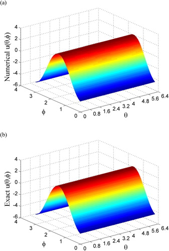
Let (47) $u=3r^2{\sin }^2\varphi -2r^2=x^2+y^2-2z^2$(47) be an exact solution of the Laplace equation in an ellipsoid with the lengths of semi-axes being a = 4, b = 3 and c = 2, which is given by (48) ${\rho }_o(\theta ,\varphi )=\frac{abc}{\sqrt{b^2{c}^2{\cos }^2\theta {\sin }^2\varphi +a^2{c}^2{\sin }^2\theta {\sin }^2\varphi +a^2{b}^2{\cos }^2\varphi }}.$(48) We take m = 8 (n = 165), $N_c=2250$, and $R_0=0.0001$, and a noise with $s=20\mathrm{\%}$. Under $\epsilon ={10}^{-5}$, the algorithm converges with 169 steps. Over the inner surface of a sphere with a radius 1.5, we plot the numerically recovered solution u in Figure 2(a), and plot the exact solution u in Figure 2(b). Upon comparing with the maximum value 4.5 of the exact solution, the maximum error $1.964\times {10}^{-1}$ is small. The value $e(u)=6.57\times {10}^{-4}$ is quite small.

Figure 2. For Example 5.1, comparing (a) numerically recovered and (b) exact boundary data on inner surface.

Example 5.2

We consider [35] (49) $\begin{array}{rl}u& =xyz+10(x+y+z)\\ & =\frac{r^3}{4}\sin (2\theta )\sin (2\varphi )\sin \varphi +10r[\cos \theta \sin \varphi +\sin \theta \sin \varphi +\cos \varphi ]\end{array}$(49) being an exact solution of the Laplace equation in a central hollow sphere, where the inner and outer radii of the spherical shell are, respectively, ${\rho }_i=1$ and ${\rho }_o=2$.

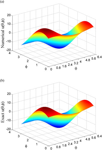
We take m = 9 (n = 220), $N_c=2250$, and $R_0=0.0001$, and a noise with $s=20\mathrm{\%}$. Under $\epsilon ={10}^{-5}$, the algorithm converges with 64 steps. Over the inner surface, we plot the numerically recovered solution u in Figure 3(a), while that of the exact solution in Figure 3(b). The maximum error 0.399 is small, upon comparing with the maximum value 17.48 of the exact solution. The value $e(u)=4.998\times {10}^{-4}$ is quite small.

Figure 3. For Example 5.2, comparing (a) numerically recovered and (b) exact boundary data on an inner sphere.

In Table 1 we list the maximum error (ME) of u on ${\mathrm{\Gamma }}_i$, $e(u)$, the CPU time and the number of steps (No. Steps) for different noise levels, where other parameters are fixed to be m = 9 (n = 220), $N_c=2250$, $R_0=0.0001$, and $\epsilon ={10}^{-5}$. It can be seen that the ME and $e(u)$ are stable and close, no matter what level of noise. The numerical method is very stable against all noises, and the CPU time is very saving, because the number of steps is small.

Table 1. For Example 5.2, comparing the maximum error (ME), $e(u)$, the CPU time and the number of steps (No. Steps) for different levels of noise.

Noise	$1\mathrm{\%}$	$5\mathrm{\%}$	$10\mathrm{\%}$	$15\mathrm{\%}$	$20\mathrm{\%}$
ME	0.374	0.379	0.386	0.393	0.399
$e(u)$	$4.970\times {10}^{-4}$	$4.975\times {10}^{-4}$	$4.981\times {10}^{-4}$	$4.989\times {10}^{-4}$	$4.998\times {10}^{-4}$
CPU time	5.85	5.79	5.65	5.65	5.60
No. Steps	51	56	60	63	64

To compare with the boundary element method (BEM) [35], Table 2 lists the ME and CPU time of the numerical results obtained by using the BEM and the present method with various noise levels. In the calculation, the BEM in conjunction with the truncated singular value decomposition-generalized cross validation (TSVD-GCV) regularization technique with 48 exact surface elements being used. We can see from Table 2 that the present method is slightly accurate than the BEM for higher noise levels. On the other hand, the BEM requires a high amount of CPU time, due to expensive numerical integration and regularization.

Table 2. For Example 5.2, comparing the ME and CPU time by using the BEM and the present method with various noise levels.

BEM [35]
Noise level	$1\mathrm{\%}$	$3\mathrm{\%}$	$5\mathrm{\%}$
ME	$3.28\times {10}^{-1}$	$5.36\times {10}^{-1}$	$5.15\times {10}^{-1}$
CPU time	112.23	112.11	112.57
Present method
ME	$3.74\times {10}^{-1}$	$3.77\times {10}^{-1}$	$3.79\times {10}^{-1}$
CPU time	5.85	5.41	5.79

Example 5.3

We give a 3D solution of the modified Helmholtz equation [37,55]: (50) $\begin{array}{rl}& \mathrm{\Delta }u-{\lambda }^{2}u=0,\\ & u(x,y,z)=\sinh (\lambda x)+\sinh (\lambda y)+\sinh (\lambda z),\end{array}$(50) which is defined in a domain Ω with the outer boundary being a sphere with a radius 2, and the inner surface is prescribed by the following spherical parametric equation: (51) $\begin{array}{rl}{\mathrm{\Gamma }}_i& =\{(x,y,z)|x={\rho }_i\cos \theta \sin \varphi ,y={\rho }_i\sin \theta \sin \varphi ,\\ z& ={\rho }_i\cos \varphi ,0\le \theta \le 2\pi ,0\le \varphi \le \pi \},\end{array}$(51) where (52) ${\rho }_i(\varphi )={[\cos (3\varphi )+\sqrt{8-{\sin }^2(3\varphi )}]}^{\frac{1}{3}}.$(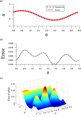52) Under $\lambda =0.5$, m = 6 (n = 84), $N_c=2250$, and $R_0=0.0001$, a noise with $s=20\mathrm{\%}$, and $\epsilon ={10}^{-5}$, 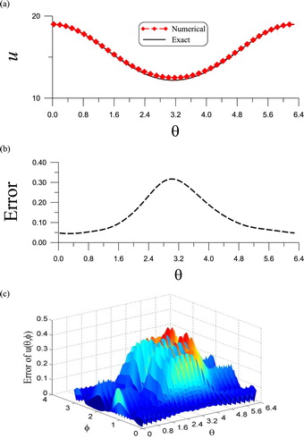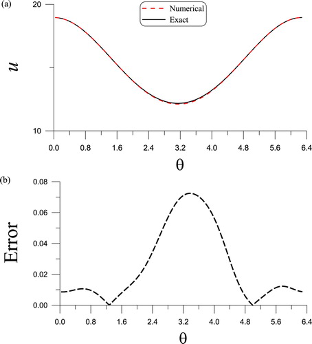the algorithm is convergence with 19 steps. Along a curve $\varphi =\pi /4$ on the inner surface, in Figure 4(a) we compare the numerically recovered and exact solutions of u, of which they are almost coincident, whose error is plotted in Figure 4(b). In Figure 4(c) we plot the error of numerically recovered solution u over the inner surface, whose maximum error is $2.926\times {10}^{-2}$, which is small, upon comparing with the maximum value 1.4 of the exact solution. The value $e(u)=3.878\times {10}^{-4}$ is quite small.

Figure 4. For Example 5.3, (a) comparing numerically recovered and exact boundary data on a curve, (b) showing error, and (c) showing error on inner surface.

In Table 3 we list the ME of u on ${\mathrm{\Gamma }}_i$, $e(u)$, the CPU time and the number of steps (No. Steps) for different noise levels, but other parameters are fixed to be m = 6 (n = 84), $N_c=2250$, $R_0=0.0001$, and $\epsilon ={10}^{-5}$.

Table 3. For Example 5.3, comparing the maximum error (ME), $e(u)$, the CPU time and the number of steps (No. Steps) for different levels of noise.

Noise	$1\mathrm{\%}$	$5\mathrm{\%}$	$10\mathrm{\%}$	$15\mathrm{\%}$	$20\mathrm{\%}$
ME	$3.079\times {10}^{-2}$	$2.987\times {10}^{-2}$	$3.964\times {10}^{-2}$	$2.944\times {10}^{-2}$	$2.926\times {10}^{-2}$
$e(u)$	$4.091\times {10}^{-4}$	$4.026\times {10}^{-4}$	$4.916\times {10}^{-4}$	$3.913\times {10}^{-4}$	$3.878\times {10}^{-4}$
CPU time	1.15	1.17	1.15	1.15	1.15
No. Steps	19	19	19	19	19

Example 5.4

We give a 3D solution of the Poisson equation: (53) $\begin{array}{rl}& \mathrm{\Delta }u=6z,\\ & u(x,y,z)=x^2+y^2-2z^2+z^3,\end{array}$(53) which is defined in a domain Ω with the outer boundary being an ellipsoid with the lengths of semi-axes being a = 5.5, b = 5.4 and c = 5.3, and the inner surface is prescribed by the following spherical parametric equation: (54) $\begin{array}{rl}{\mathrm{\Gamma }}_i& =\{(x,y,z)|x={\rho }_i\cos \theta \sin \varphi ,y={\rho }_i\sin \theta \sin \varphi ,\\ z& ={\rho }_i\cos \varphi ,0\le \theta \le 2\pi ,0\le \varphi \le \pi \},\end{array}$(54) where (55) ${\rho }_i(\theta ,\varphi )=(3.2+0.2\cos \theta ){[\cos (3\varphi )+\sqrt{8-{\sin }^2(3\varphi )}]}^{\frac{1}{3}}.$(55) Under m = 7 (n = 120), $N_c=2250$, and $R_0=0.001$, a noise with $s=20\mathrm{\%}$, and $\epsilon ={10}^{-5}$, the algorithm is convergence with 327 steps. 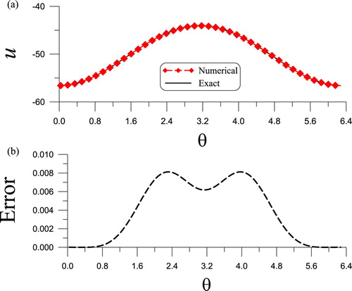Along a curve $\varphi =\pi /4$ on the inner surface, in Figure 5(a) we compare the numerically recovered and exact solutions of u, of which they are close and the error is plotted in Figure 5(b). In Figure 5(c) we plot the error of numerically recovered solution u over the inner surface, of which the ME 0.796 is small, upon comparing with the maximum value 106.44 of the exact solution. The value $e(u)=8.897\times {10}^{-5}$ is very small.

Figure 5. For Example 5.4, (a) comparing numerically recovered and exact boundary data on a curve, (b) showing error, and (c) showing error on inner surface.

The factor $R_0$ plays the role as a regularization parameter. In Table 4 we list the ME of u on ${\mathrm{\Gamma }}_i$, $e(u)$, and the number of steps (No. Steps) for different $R_0$, but other parameters are fixed to be m = 7 (n = 120), $N_c=2250$, and $\epsilon ={10}^{-5}$.

Table 4. For Example 5.4, comparing the maximum error (ME), $e(u)$, and the number of steps (No. Steps) for different values of $R_0$.

$R_0$	$s_{ijk}=1$	10	1	0.1	0.01	0.001
ME	1.228	0.808	0.808	0.808	0.808	0.796
$e(u)$	$1.270\times {10}^{-4}$	$9.007\times {10}^{-5}$	$9.007\times {10}^{-5}$	$9.007\times {10}^{-5}$	$9.007\times {10}^{-5}$	$8.897\times {10}^{-5}$
No. Steps	over 5000	538	485	436	409	327

From Table 4 we can see that the ME and $e(u)$ are stable, which are not sensitive to the value of $R_0$; however, smaller $R_0$ leads to faster convergence with the number of steps smaller. If we do not consider the regularization with $s_{ijk}=1$, the algorithm will lead to large numerical error and does not converge within 5000 steps.

Example 5.5

Under the same geometric configuration as that in Example 5.4, here we give a 3D solution of a strong convection diffusion equation: (56) $\begin{array}{rl}& \mathrm{\Delta }u-5u_r=5[4r-6r{\sin }^2\varphi ],\\ & u(x,y,z)=3r^2{\sin }^2\varphi -2r^2.\end{array}$(56) Under m = 9 (n = 220), $N_c=2250$, and $R_0=0.0001$, a noise with $s=20\mathrm{\%}$, and $\epsilon ={10}^{-5}$, the algorithm is convergence with 311 steps. 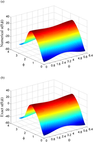Along a curve $\varphi =0$ on the inner surface, in Figure 6(a) we compare the numerically recovered and exact solutions of u, which are very close and the error is plotted in Figure 6(b).

Figure 6. For Example 5.5, (a) comparing numerically recovered and exact boundary data on a curve, and (b) showing error.

In Figures 7(a,b) we plot the numerically recovered solution and exact solution over the inner surface. The maximum error $3.738\times {10}^{-2}$ is very small, upon comparing with the maximum value 54.34 of the exact solution. The value $e(u)=1.371\times {10}^{-5}$ is very small.

Figure 7. For Example 5.5, comparing (a) numerically recovered and (b) exact boundary data on inner surface.

In Table 5 we list the ME of u on ${\mathrm{\Gamma }}_i$, $e(u)$, the CPU time and the number of steps (No. Steps) for different noise levels, and other parameters are fixed to be m = 9 (n = 220), $N_c=2250$, $R_0=0.0001$, and $\epsilon ={10}^{-5}$.

Table 5. For Example 5.5, comparing the maximum error (ME), $e(u)$, the CPU time and the number of steps (No. Steps) for different levels of noise.

Noise	$1\mathrm{\%}$	$5\mathrm{\%}$	$10\mathrm{\%}$	$15\mathrm{\%}$	$20\mathrm{\%}$
ME	$2.648\times {10}^{-2}$	$2.968\times {10}^{-2}$	$3.310\times {10}^{-2}$	$3.666\times {10}^{-2}$	$3.738\times {10}^{-2}$
$e(u)$	$1.046\times {10}^{-5}$	$1.099\times {10}^{-5}$	$1.169\times {10}^{-5}$	$1.272\times {10}^{-5}$	$1.371\times {10}^{-5}$
CPU time	25.56	25.67	25.58	25.50	25.34
No. Steps	317	317	319	319	311

From Table 5 we can see that the ME and $e(u)$ are stable, which are slightly increased when the level of noise is increased. The numerical method is very stable against all noises, and the CPU time is very saving, because the number of steps is small.

Example 5.6

We give a 3D solution of the Helmholtz equation: (57) $\begin{array}{rl}& \mathrm{\Delta }u+{\lambda }^{2}u=0,\\ & u(x,y,z)=\sin (\lambda x)+\sin (\lambda y)+\sin (\lambda z).\end{array}$(57) The domain Ω is same with that in Example 5.3.

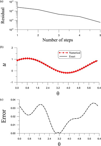
Under $\lambda =0.5$, m = 2 (n = 10), $N_c=2250$, and $R_0=0.0001$, a biased noise with $\sigma =20\mathrm{\%}$, and $\epsilon ={10}^{-5}$, the algorithm is convergence with 4 steps as shown in Figure 8(a). Along a curve $\varphi =\pi /4$ on the inner surface, in Figure 8(b) we compare the numerically recovered and exact solutions of u, of which the ME is $4.358\times {10}^{-2}$ and $e(u)$ is $8.345\times {10}^{-4}$. The numerical error is plotted in Figure 8(c). Upon imposing the biased noise with $\sigma =20\mathrm{\%}$, the ME is $5.172\times {10}^{-2}$ and $e(u)$ is $9.999\times {10}^{-4}$, which are slightly larger than that with uniform noise $s=20\mathrm{\%}$.

Figure 8. For Example 5.6, (a) convergence rate, (b) comparing numerically recovered and exact boundary data on a curve, and (c) showing error.

However, when λ is increased to 1.5, it needs 8 steps, the ME is also increased to $7.004\times {10}^{-1}$ and $e(u)$ is increased to $5.435\times {10}^{-3}$. For the inverse Cauchy problem with a higher wave number in the Helmholtz equation, it is very difficult to recover the unknown data on the inner surface.

Example 5.7

We give a 3D solution of the varying coefficient convection diffusion equation: (58) $\begin{array}{rl}& u_{xx}+u_{yy}+u_{zz}+xyz{u}_x+y{u}_y=6z+2x^{2}yz+2y^2,\\ & u(x,y,z)=x^2+y^2-2z^2+z^3,\end{array}$(58) of which the domain Ω is same with that in Example 5. 4.

Under m = 7 (n = 120), $N_c=2250$, and $R_0=0.001$, a noise with $s=20\mathrm{\%}$, and $\epsilon ={10}^{-5}$, the algorithm is convergence with 666 steps. Along a curve $\varphi =\pi /4$ on the inner surface, in Figure 9(a) we compare the numerically recovered and exact solutions of u, of which they are close and the error is plotted in Figure 9(b). The ME 0.243 is small, upon comparing with the maximum value 106.44 of the exact solution, while the value $e(u)=2.627\times {10}^{-5}$ is very small.

Figure 9. For Example 5.7, (a) comparing numerically recovered and exact boundary data on a curve, and (b) showing error.

In Table 6 we list the ME of u on ${\mathrm{\Gamma }}_i$, $e(u)$, and the number of steps (No. Steps) for different $R_0$, but other parameters are fixed to be m = 7 (n = 120), $N_c=2250$, and $\epsilon ={10}^{-5}$.

Table 6. For Example 5.7, comparing the maximum error (ME), $e(u)$, and the number of steps (No. Steps) for different values of $R_0$.

$R_0$	10	1	0.1	0.01	0.001	0.0001
ME	0.248	0.248	0.248	0.249	0.243	0.276
$e(u)$	$2.662\times {10}^{-5}$	$2.662\times {10}^{-5}$	$2.662\times {10}^{-5}$	$2.658\times {10}^{-5}$	$2.627\times {10}^{-5}$	$2.687\times {10}^{-5}$
No. Steps	1111	1048	1002	879	666	458

From Table 6 we can see that the ME and $e(u)$ are not sensitive to the value of $R_0$; however, smaller $R_0$ leads to faster convergence with the number of steps smaller.

6. Conclusions

In the paper, we have solved the 3D inverse Cauchy problems of the elliptic type linear PDEs in the closed walled shells to recover the unknown inner boundary data. A major novelty is setting up a new numerical method to solve the inverse Cauchy problems through the technique of homogenization function, which annihilates both the Dirichlet and Neumann data over-specified on the outer boundary. After a homogenization technique, the numerical solution of the transformed variable was expressed in terms of boundary functions as the bases, which automatically satisfy the homogeneous Cauchy boundary conditions on the outer boundary. The unknown data on the inner surface can be recovered fast by solving a linear equations system. The new method is quite simple and very time saving, because we have developed a direct collocation method to solve the inverse Cauchy problems, determining v by solving a direct problem and then determining the unknown boundary data by Equation (43(43) $u(\mathbf{x})=v(\mathbf{x})+B^0(r={\rho }_i,\theta ,\varphi ),\mathbf{x}\in {\mathrm{\Gamma }}_i.$(43) ). In doing so, the numerical solution of u automatically satisfies the over-specified Cauchy data on the outer surface. Several examples of the Laplace equation, the Helmholtz equation, the modified Helmholtz equation, the Poisson equation, a strong convection diffusion equation and a varying coefficient elliptic equation, confirmed the efficiency and accuracy of the presented numerical method. Although under a large noise up to $20\mathrm{\%}$, the new method was robust to achieve quite accurate solutions of the inner boundary data. The key point for the success of the presented homogenization/boundary function method in the solutions of the inverse Cauchy problems in the three-dimension domains is the derivation of a new homogenization function $B^0$ as shown by Equation (31(31) $B^0(r,\theta ,\varphi )=h(\theta ,\varphi )+[r-{\rho }_o(\theta ,\varphi )]u_{{\rho }_o}({\rho }_o,\theta ,\varphi ),$(31) ) in Theorem 3.2, and the boundary functions in Equation (37(37) $B^{ijk}(\mathbf{x})=x^{i-j}{y}^{j-k}{z}^k{E}^0(\mathbf{x}),i\ge 0,0\le j\le i,0\le k\le j,$(37) ), which are adopted as the bases of numerical solution. In order to accelerate the convergence, smaller regularization parameter $R_0$ is better than larger ones.

Acknowledgements

The authors highly appreciate the constructive comments from anonymous referees, which improved the quality of this paper.

Disclosure statement

No potential conflict of interest was reported by the authors.

References

- Belgacem FB. Why is the Cauchy problem severely ill-posed? Inverse Probl. 2007;23:823–836. doi: 10.1088/0266-5611/23/2/020
- Borachok I, Chapko R, Johansson BT. Numerical solution of an elliptic 3-dimensional Cauchy problem by the alternating method and boundary integral equations. J Inv Ill-posed Prob. 2016;24:711–725.
- Berntsson F, Eldén L. Numerical solution of a Cauchy problem for the Laplace equation. Inverse Probl. 2001;17:839–853. doi: 10.1088/0266-5611/17/4/316
- Qian Z, Fu CL, Li ZP. Two regularization methods for a Cauchy problem for the Laplace equation. J Math Anal Appl. 2008;338:479–489. doi: 10.1016/j.jmaa.2007.05.040
- Hao DN, Hien PM. Stability results for the Cauchy problem for the Laplace equation in a strip. Inverse Probl. 2003;19:833–844. doi: 10.1088/0266-5611/19/4/303
- Marin L, Elliott L, Heggs PJ, et al. The method of fundamental solutions for the Cauchy problem associated with two-dimensional Helmholtz-type equations. Comput Struct. 2005;83:267–278. doi: 10.1016/j.compstruc.2004.10.005
- Qin HH, Wei T. Modified regularization method for the Cauchy problem of the Helmholtz equation. Appl Math Model. 2009;33:2334–2348. doi: 10.1016/j.apm.2008.07.005
- Xiong XT. A regularization method for a Cauchy problem of the Helmholtz equation. J Comput Appl Math. 2010;233:1723–1732. doi: 10.1016/j.cam.2009.09.001
- Qian AL, Xiong XT, Wu YJ. On a quasi-reversibility regularization method for a Cauchy problem of the Helmholtz equation. J Comput Appl Math. 2010;233:1969–1979. doi: 10.1016/j.cam.2009.09.031
- Regi'nska T, Wakulicz A. Wavelet moment method for the Cauchy problem for the Helmholtz equation. J Comput Appl Math. 2009;223:218–229. doi: 10.1016/j.cam.2008.01.005
- Fu CL, Li HF, Qian Z, et al. Fourier regularization method for solving a Cauchy problem for the Laplace equation. Inv Prob Sci Eng. 2008;16:159–169. doi: 10.1080/17415970701228246
- Fu CL, Feng XL, Qian Z. The Fourier regularization for solving the Cauchy problem for the Helmholtz equation. Appl Numer Math. 2009;59:2625–2640. doi: 10.1016/j.apnum.2009.05.014
- Lesnic D, Elliott L, Ingham DB. An iterative boundary element method for solving numerically the Cauchy problem for the Laplace equation. Eng Anal Bound Elem. 1997;20:123–133. doi: 10.1016/S0955-7997(97)00056-8
- Mera NS, Elliott L, Ingham DB, et al. An iterative boundary element method for the solution of a Cauchy steady state heat conduction problem. Comput Model Eng Sci. 2000;1:101–106.
- Jin B, Zheng Y. A meshless method for some inverse problems associated with the Helmholtz equation. Comput Meth Appl Mech Eng. 2006;195:2270–2288. doi: 10.1016/j.cma.2005.05.013
- Chapko R, Kress R. A hybrid method for inverse boundary value problems in potential theory. J Inv Ill-Posed Prob. 2005;13:27–40. doi: 10.1515/1569394053583711
- Chakib A, Nachaoui A. Convergence analysis for finite element approximation to an inverse Cauchy problem. Inverse Probl. 2006;22:1191–1206. doi: 10.1088/0266-5611/22/4/005
- Rischette R, Baranger TN, Andrieux S. Regularization of the noisy Cauchy problem solution approximated by an energy-like method. Int J Numer Mthod. Eng. 2013;95:271–287. doi: 10.1002/nme.4501
- Liu CS, Wang F, Gu Y. A Trefftz/MFS mixed-type method to solve the Cauchy problem of the Laplace equation. Appl Math Lett. 2019;87:87–92. doi: 10.1016/j.aml.2018.07.028
- Liu CS, Cahng CW. An energy regularization of the MQ-RBF method for solving the Cauchy problems of diffusion-convection-reaction equations. Commun Nonlinear Sci Numer Simul. 2019;67:375–390. doi: 10.1016/j.cnsns.2018.07.002
- Payne LE. Improperly posed problems in partial differential equations. Regional Conference Series in Applied Mathematics, Vol.22, Philadelphia (PA): SIAM; 1975.
- Tikhonov AN, Goncharsky AV, Stepanov VV, et al. Numerical methods for the solution of Ill-posed Problems. Dordrecht: Kluwer Academic Publishers; 1995. (Mathematics and its Applications, Vol. 328).
- Wei T, Hon YC, Ling T. Method of fundamental solutions with regularization techniques for Cauchy problems of elliptic operators. Eng Anal Bound Elem. 2007;31:373–385. doi: 10.1016/j.enganabound.2006.07.010
- Jourhmane M, Nachaoui A. An alternating method for an inverse Cauchy problem. Num Algor. 1999;21:247–260. doi: 10.1023/A:1019134102565
- Jourhmane M, Nachaoui A. Convergence of an alternating method to solve the Cauchy problem for Poisson's equation. Appl Anal. 2002;81:1065–1083. doi: 10.1080/0003681021000029819
- Essaouini M, Nachaoui A, Hajji SE. Numerical method for solving a class of nonlinear elliptic inverse problems. J Comput Appl Math. 2004;162:165–181. doi: 10.1016/j.cam.2003.08.011
- Jourhmane M, Lesnic D, Mera NS. Relaxation procedures for an iterative algorithm for solving the Cauchy problem for the Laplace equation. Eng Anal Bound Elem. 2004;28:655–665. doi: 10.1016/j.enganabound.2003.07.002
- Marin L, Lesnic D. The method of fundamental solutions for the Cauchy problem associated with two-dimensional Helmholtz-type equations. Comput Struct. 2005;83:267–278. doi: 10.1016/j.compstruc.2004.10.005
- Marin L, Elliott L, Heggs PJ et al. Conjugate gradient-boundary element solution to the Cauchy problem for Helmholtz-type equations. Comput Mech. 2003;31:367–377. doi: 10.1007/s00466-003-0439-y
- Qin HH, Wen DW. Tikhonov type regularization method for the Cauchy problem of the modified Helmholtz equation. Appl Math Comput. 2008;203:617–628.
- Qin HH, Wei T. Quasi-reversibility and truncation methods to solve a Cauchy problem for the modified Helmholtz equation. Math Comput Simul. 2009;80:352–366. doi: 10.1016/j.matcom.2009.07.005
- Marin L, Elliott L, Heggs PJ, et al. BEM solution for the Cauchy problem associated with Helmholtz-type equations by the Landweber method. Eng Anal Bound Elem. 2004;28:1025–1034. doi: 10.1016/j.enganabound.2004.03.001
- Wei T, Hon YC, Cheng J. Computation for multidimensional Cauchy problem. SIAM J Contr Optim. 2003;42:381–396. doi: 10.1137/S0363012901389391
- Marin L. A meshless method for the numerical of the Cauchy problem associated with three-dimensional Helmholtz-type equations. Appl Math Comput. 2005;165:355–374.
- Wang F, Chen W, Qu W, et al. A BEM formulation in conjunction with parametric equation approach for three-dimensional Cauchy problems of steady heat conduction. Eng Anal Bound Elem. 2016;63:1–14. doi: 10.1016/j.enganabound.2015.10.007
- Liu CS. A simple Trefftz method for solving the Cauchy problems of three-dimensional Helmholtz equation. Eng Anal Bound Elem. 2016;63:105–113. doi: 10.1016/j.enganabound.2015.11.009
- Liu CS, Qu W, Chen W, et al. A novel Trefftz method of the inverse Cauchy problem for 3D modified Helmholtz equation. Inv Prob Sci Eng. 2017;25:1278–1298. doi: 10.1080/17415977.2016.1247449
- Liu CS, Wang F, Qu W. Fast solving the Cauchy problems of Poisson equation in an arbitrary three-dimensional domain. Comput Model Eng Sci. 2018;114:351–380.
- Lin J, Liu CS, Chen W et. al. A novel Trefftz method for solving the multi-dimensional direct and Cauchy problems of Laplace equation in an arbitrary domain. J Comput Sci. 2018;25:16–27. doi: 10.1016/j.jocs.2017.12.008
- Liu CS, Chang CW. Solving the 3D Cauchy problems of nonlinear elliptic equations by the superposition of a family of 3D homogenization functions. Eng Anal Bound Elem. 2019;105:122–128. doi: 10.1016/j.enganabound.2019.04.001
- Liu CS, Kuo CL. A multiple-scale Pascal polynomial triangle solving elliptic equations and inverse Cauchy problems. Eng Anal Bound Elem. 2016;62:35–43. doi: 10.1016/j.enganabound.2015.09.003
- Liu CS, Young DL. A multiple-scale Pascal polynomial for 2D Stokes and inverse Cauchy-Stokes problems. J Comput Phys. 2016;312:1–13. doi: 10.1016/j.jcp.2016.02.017
- Liu CS. A two-side equilibration method to reduce the condition number of an ill-posed linear system. Comput Model Eng Sci. 2013;91:17–42.
- Liu CS. An equilibrated method of fundamental solutions to choose the best source points for the Laplace equation. Eng Anal Bound Elem. 2012;36:1235–1245. doi: 10.1016/j.enganabound.2012.03.001
- Liu CS. Optimally scaled vector regularization method to solve ill-posed linear problems. Appl Math Comput. 2012;218:10602–10616.
- Liu CS. The pre/post equilibrated conditioning methods to solve Cauchy problems. Eng Anal Bound Elem. 2014;40:62–70. doi: 10.1016/j.enganabound.2013.11.017
- Ku CY, Kuo CL, Fan CM et al. Numerical solution of three-dimensional Laplacian problems using the multiple scale Trefftz method. Eng Anal Bound Elem. 2015;50:157–168. doi: 10.1016/j.enganabound.2014.08.007
- Lv H, Hao F, Wang Y, et al. The MFS versus the Trefftz method for the Laplace equation in 3D. Eng Anal Bound Elem. 2017;83:133–140. doi: 10.1016/j.enganabound.2017.06.006
- Liu CS, Liu D. Optimal shape parameter in the MQ-RBF by minimizing an energy gap functional. Appl Math Lett. 2018;86:157–165. doi: 10.1016/j.aml.2018.06.031
- Wang F, Liu CS, Qu W. Optimal sources in the MFS by minimizing a new merit function: Energy gap functional. Appl Math Lett. 2018;86:229–235. doi: 10.1016/j.aml.2018.07.002
- Liu CS, Chen YW, Chang JR. The Trefftz test functions method for solving the generalized inverse boundary value problems of Laplace equation. J Marine Sci Tech. 2018;26:638–647.
- Liu CS, Wang F. An energy method of fundamental solutions for solving the inverse Cauchy problems of the Laplace equation. Comput Math Appl. 2018;75:4405–4413. doi: 10.1016/j.camwa.2018.03.038
- Liu CS, Wang F, Gu Y. Trefftz energy method for solving the Cauchy problem of the Laplace equation. Appl Math Lett. 2018;79:187–195. doi: 10.1016/j.aml.2017.12.013
- Liu CS, Wang F. A meshless method for solving the nonlinear inverse Cauchy problem of elliptic type equation in a doubly-connected domain. Comput Math Appl. 2018;76:1837–1852. doi: 10.1016/j.camwa.2018.07.032
- Lin J, Chen CS, Liu CS. Fast solution of three-dimensional modified Helmholtz equations by the method of fundamental solutions. Commun Comput Phys. 2016;20:512–533. doi: 10.4208/cicp.060915.301215a