Reconstruction algorithm for 3D Compton scattering imaging with incomplete data

Abstract

Compton scattering describes the scattering of a photon after its collision with an electron. The recent developments of spectral cameras, able to collect photons in terms of energy, open the way to a new imaging concept: 3D Compton scattering imaging (CSI), which seeks to exploit the scattered radiation as a vector of information while a specimen of interest is illuminated by a monochromatic ionizing source. Focusing on modelling the first-order scattering, image reconstruction from CSI data remains a difficult challenge. In particular, physical constraints (detector and architecture of the scanner) lead to various incompleteness scenario within the data and thus streak artifacts when using filtered backprojection type formulas. This paper addresses the problem of recovering an object under study using CSI data subject to incompleteness and assuming only first-order scattering. The proposed method consists of suitably tuning the multiplicative Kaczmarz algorithm and is implemented and tested for two architectures of the scanner. Furthermore, the modality on CSI considered here presents the advantage of not requiring any rotation of the source or object.

Keywords:

• Compton scattering
• image reconstruction
• incomplete data
• expectation maximization
• total variation

2010 Mathematics Subject Classifications:

• 65R10
• 44A12

1. Introduction

Since the advent of Computerized Tomography (CT), many 3D imaging concepts have emerged and applications relying on imaging have grown. One can mention Single Photon Emission CT, Positron Emission Tomography or Cone-Beam CT for the standard 3D imaging systems based on an ionizing source. In these configurations, the energy discrimination has very limited use but the idea of exploiting it in order to enhance the image quality, optimize the acquisition processor to compensate for some limitations (such as limited angle issues) has led to various works [1–8]. However, the energy has been used to provide additional information in these imaging modalities (e.g. spectral or dual-energy CT).

The recent development of high-energy resolution cameras, i.e. able to bin detected photons in terms of energy, offers the possibility to consider the spectrum of the measured photons as a vector of information in the same way as the source/detector positions in classical CT. After many works in the two last decades, see [9–14], such cameras reach a spatial resolution of 1 mm and are able to detect with an energy resolution of 1% of its full width at half maximum (FWHM). Depending on the energy level and on the different materials, recent cameras can detect with a resolution $\mathrm{\Delta }E$ under 1 keV at 140 keV and around 5 keV at 600–700 keV. Below in the simulations, we consider energy resolutions and dimensions of the same order of magnitude for the camera.

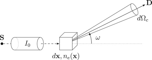
The Compton scattering is the collision between a photon (of a given energy $E_0$) and an electron. The photon gives a part of its energy to the electron producing its recoil and is then scattered with an angle ω with respect to its incident angle, see Figure 1. The Compton formula [15] gives the energy after collision in terms of the incoming energy $E_0$ and the scattering angle ω, (1) $E_{\omega }=\frac{E_0}{1+{\displaystyle \frac{E_0}{m_e{c}^2}}(1-\cos \omega )},$(1) where $\omega \in [0,\pi ]$ is the scattering angle and $m_e{c}^2=0.511$ MeV represents the energy of an electron at rest. This phenomenon is one of the interactions between photons and matter responsible for the attenuation of a photon beam crossing a medium and is dominant on the large range [26 keV, 26 MeV], see [16], varying with the type of materials under study. When the ionizing source is monochromatic, i.e. emitting essentially at one energy, the loss in energy of the emitted radiation can thus be related with the scattering angle as a consequence of the Compton effect.

Figure 1. Geometry of Compton scattering: the incident photon energy $E_0$ yields a part of its energy to an electron and is scattered with an angle ω.

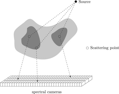
The use of the scattered radiation via suited spectral cameras opens the way to an innovative 3D imaging concept, Compton scattering imaging (abbreviated here by CSI). A general concept is depicted in Figure 2. A monochromatic ionizing source illuminates an object and a set of spectral cameras measure the spectrum of the measured photons for different positions. Although the technology involved in imaging the scattered radiation has not yet reached the same level of maturity as the one used in conventional imaging (CT, SPECT, PET), scientists have proposed and studied in the last decades different bi-dimensional systems, called Compton scattering tomography (CST), see, e.g. [17–32]. More recently, an important application was proposed in radiation oncology for treatment planning (the electron density is known as reliable information) and image guidance/patient setup for treatments, see [33,34]. It is also possible to consider interior sources, for instance via the insertion of radiotracers like in SPECT. Then considering collimated detectors, it is possible to model the scattered flux through conical Radon transforms, see for instance [35,36]. In this work, we consider only systems with external sources. However, one can notice many similarities to the imaging processes considered for internal source imaging (e.g. SPECT) where the source origin is unknown and scatter imaging with an external source (as discussed in this work) where the scatter origin is unknown.

Figure 2. Working principle of systems on 3D CSI.

Equation (1(1) $E_{\omega }=\frac{E_0}{1+{\displaystyle \frac{E_0}{m_e{c}^2}}(1-\cos \omega )},$(1) ) gives a geometric interpretation of the scattered radiation. This is depicted in Figure 3. Considering a monochromatic source S emitting photons of given energy $E_0$ and a detector D, then the Compton formula tells that the photons detected at a given energy $E_{\omega }$ were scattered by the illuminated medium at points M such that $\widehat{\mathbf{S}\mathbf{M}\mathbf{D}}=(\pi -\omega )$. This set of points characterizes a unique spindle torus, noted $\mathfrak{T}(\theta ,E_{\omega })$, in which $\theta =\overrightarrow{\mathbf{S}\mathbf{D}}/\parallel \overrightarrow{\mathbf{S}\mathbf{D}}\parallel$. More precisely, when $\omega \in [0,\frac{\pi }{2}]$ the manifold refers to the inside part – lemon – of the spindle torus and when $\omega \in [\frac{\pi }{2},\pi ]$ it refers to the outside part – apple – see Figure 3.

Figure 3. A complete spindle torus (left), its inside part often called lemon (middle) and its outside part often called apple (right) for a given scattering angle $\omega \in [0,\pi /2]$. The lemon (middle) represents the torus $\mathfrak{T}(\theta ,E_{\omega }),$ whereas the apple (right) represents the torus $\mathfrak{T}(\theta ,E_{\pi -\omega })$.

Multiple-order scattering, i.e. photons scattered more than once, occurs in practice and represents a major challenge. Indeed, the geometric representation described above assumes that the detected photons incoming with energy $E_{\omega }$ were scattered only once. Thereby, multiple-order scattering turns out to be difficult to model and thus to handle. In this paper, we focus on the first-order scattering by assuming that the multiple scattering was corrected. To do so, a prior information on the studied medium can be considered to compute the part of the multiple scattering and subtract it from the CSI measurement. The residual error would then be treated as a component of noise which is understood here as the whole perturbation and thus as a composition of noise (Poisson) and model uncertainty. In the same spirit, the multiple scattering shall be substantially reduced paradoxically by reducing that part of the Compton effect. One can imagine both the following configurations (see Section 5) in order to theoretically reduce the contribution of multiple scattering.

• In the first case, we exploit the dominance curve of the attenuation phenomena by considering an initial energy $E_0$ around the inflection point of the dominance photoelectric absorption/Compton scattering. In a medical/human body context, the energy $E_0$ could be chosen at <80 keV. This setting reduces the chance of Compton scattering but more specifically of multiple scattering. Indeed, the first-order scattered photons lose a part of their energy falling into the dominance part of the photoelectric absorption and reducing by the same way the occurrence of multiple scattering. The drawback of this approach is to sacrifice the number of scattered photons requiring a longer acquisition time in order to limit the share of multiple scattering and thus to ensure the toric representation. This configuration would fit with medical applications.

• The second configuration consists in increasing the emission energy $E_0$ for the purpose of favouring the scattered radiation considering slim objects to image leading to a reduction in the impact of the attenuation factor and thus the chance of multiple scattering. This configuration has the advantage to limit the photoelectric effect and thus to increase the detection ratio but also restrict the size and shape of the objects under study. This configuration would fit with non-destructive testing applications, for pre-clinical trials when studying small animals or as a complement to microscopy applications. It may also apply to radiation therapy applications (e.g. when using Cs137, or even potentially Co60 which is not monoenergetic but maybe close enough with only two-photon energies).

Both cases rely on the dominance of the attenuation curves regarding Compton scattering and photoelectric absorption. These curves are quite smooth and even though the transition is arbitrarily assumed to be at 80 keV, the relative probabilities will not actually vary greatly when choosing 70 keV vs. 90 keV for instance.

The measurement of the scattered radiation carries information of the scattering sites and thus of the density of electrons. Therefore, the development of 3D CSI modalities involves the following inverse problem: to model the acquisition step under the form $\mathcal{T}{n}_e=g$ and then recover the electron density map $n_e$. A closed-form inversion formula for such a family of operators does not exist to the best of our knowledge. However, in [37] we proposed the study of a generalized Radon transforms on a family of surfaces suited for the tori observed in CSI. In particular, we gave a reconstruction formula which was proven to preserve the contours of the electron density. The contours are the singularities of the object, i.e. where the object is not smooth. In most applications, the objects are piecewise constant or smooth and thus the contours or singularities represent its edges. They are simply displayed by application of some differential operators such as the gradient or the Laplacian. However, the reconstruction technique cannot handle incomplete data, see Figure 10. Indeed, we will see that the architectural and technological constraints will lead to limitations in the data. In order to circumvent the well-known streak artifacts like in the limited angle case in CT, we propose to apply an iterative algorithm. We selected a multiplicative Kaczmarz (also called ordered subset expectation maximum-likelihood ‘OSEM’ algorithm) algorithm first due to its robustness to Poisson noise but also due to its fast convergence. However, we will see that the forward operator $\mathcal{T}$ is strongly connected to the electron density and thence cannot be fully known. To solve this issue, we modified the OSEM algorithm to fit with the reconstruction problem in 3D CSI.

Section 2 shows how the data in CSI can be modelled by a weighted toric Radon transform neglecting or at least considering as noise the multiple scattering. In Section 3, we propose two architectures for CSI modalities and discuss incomplete data issues. We propose a designed algorithm for CSI data in Section 4. The algorithm corresponds to a modified multiplicative Kaczmarz algorithm combined with a step of total-variation regularization. The choice of these techniques is motivated by the systematic presence of Poisson noise due to the emission process and the scattering process. Finally, Section 5 deals with the simulation results on the different modalities with each configuration considering Poisson noise and incomplete data on two test phantoms. The first phantom is the classical Shepp–Logan phantom in 3D with low-contrast and the second one is a slim board symbolizing potential non-destructive testing applications. A conclusion ends the manuscript.

2. Modelling based on a weighted toric Radon transform

We consider a monochromatic ionizing source S and a detector D able to collect incoming photons in terms of energy. We also assume that the photons are scattered only once as discussed in the Introduction. We denote by $\mathbf{s}$, $\mathbf{d}$ and $\mathbf{x}$ the coordinates of the points S, D and M. Then, the variation of the number of photons $N_c$ detected at D and scattered at M in a solid angle $d{\mathrm{\Omega }}_c$ along a direction making an angle ω with the incoming flux, see Figure 1, can be quantified as (2) $\frac{{\mathrm{d}}^2{N}_c}{\mathrm{d}\mathbf{x}\mathrm{d}{\mathrm{\Omega }}_c}=\frac{I_0{r}_e^2}{4}P\left(\omega \right)\frac{A_0(\mathbf{s},\mathbf{x})A_{\omega }(\mathbf{x},\mathbf{d})}{\parallel \mathbf{s}-\mathbf{x}{\parallel }^2\parallel \mathbf{x}-\mathbf{d}{\parallel }^2}{n}_e(\mathbf{x}\mathbf{)},$(2) with $I_0$ the intensity of the emitted flux, $P\left(\omega \right)$ the Klein–Nishina probability [38], $r_e$ the classical radius of an electron, $n_e\left(\mathbf{x}\right)$ the electron density at point $\mathbf{x}$ and $A_0(\mathbf{s},\mathbf{x})$ (resp., $A_{\omega }(\mathbf{x},\mathbf{d})$) the attenuation factor with photometric dispersion before (resp., after) scattering. The attenuation factor between two points $\mathbf{x}$ and $\mathbf{y}$ can be expressed through the well-known Beer–Lambert law, i.e. $A_{\omega }(\mathbf{x},\mathbf{y})=\exp \left(-\parallel \mathbf{y}-\mathbf{x}\parallel {\int }_0^1{\mu }_{\omega }\left(\mathbf{x}+t\frac{(\mathbf{y}-\mathbf{x})}{\parallel \mathbf{y}-\mathbf{x}\parallel }\right)\mathrm{d}t\right)$ in which ${\mu }_{\omega }$ is the lineic attenuation at energy $E_{\omega }$. As seen in the Introduction, the set of point M for a given scattering angle ω belongs to the lemon (resp., apple) part of a spindle torus for $\omega <\pi /2$ (resp., $\omega >\pi /2$). In the following, we assume that D is a point detector, i.e. its size is sufficiently small to ensure that each point M (in practice each voxel) is uniquely determined for the scattering angles ω and has an open aperture sufficient to collect the scattered photons. Thereby, the intensity of detected scattered photons at D with energy $E_{\omega }$ is after integration along the torus $\mathfrak{T}$ proportional to ${\int }_{\mathbf{x}\in \mathfrak{T}}\frac{A_0(\mathbf{s},\mathbf{x})A_{\omega }(\mathbf{x},\mathbf{d})}{\parallel \mathbf{s}-\mathbf{x}{\parallel }^2\parallel \mathbf{x}-\mathbf{d}{\parallel }^2}{n}_e(\mathbf{x}\mathbf{)}\mathrm{d}\mathbf{x}.$ One recognizes the weighted Radon transform of the electron density $n_e$ along the lemon or apple part of the spindle torus $\mathfrak{T}$. 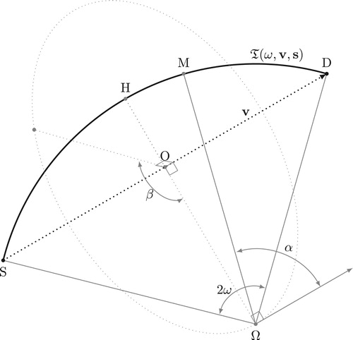We recall here some results from [37]. Let us define $\mathbf{v}=\mathbf{d}-\mathbf{s}\in \mathbb{V}$. Trigonometric identities lead to the surface illustrated in Figure 4 to be represented as the set (3) $\mathfrak{T}(\omega ,\mathbf{v},\mathbf{s})=\left\{\mathbf{s}+\frac{\parallel \mathbf{v}\parallel }{2\sin \omega }{R}_{\mathbf{v}}\mathbf{u}(\alpha ,\text{β}):\alpha \in [-\omega +\pi /2,\omega +\pi /2],\text{β}\in [0,2\pi ]\right\}$(3) with $\mathbf{u}(\alpha ,\text{β})=\left(\begin{array}{c}(\sin \alpha -\cos \omega )\cos \text{β}\\ (\sin \alpha -\cos \omega )\sin \text{β}\\ \cos \alpha +\sin \omega \end{array}\right)$ and $R_{\mathbf{v}}$ the rotation matrix induced by the vector $\mathbf{v}$ which using our convention is $R_{\mathbf{v}}=\left(\begin{array}{ccc}\cos \psi \cos \varphi & -\sin \varphi & \sin \psi \cos \varphi \\ \cos \psi \sin \varphi & \cos \varphi & \sin \psi \sin \varphi \\ -\sin \psi & 0& \cos \psi \end{array}\right)$ in which ψ and ϕ stand for the polar and azimuthal angles associated with $\mathbf{v}/\parallel \mathbf{v}\parallel$, i.e. $\frac{\mathbf{v}}{\parallel \mathbf{v}\parallel }=\left(\begin{array}{c}\sin \psi \cos \varphi \\ \sin \psi \sin \varphi \\ \cos \psi \end{array}\right).$ With the variables $(\omega ,\mathbf{v},\mathbf{s})$, the inverse problem associated to the measurement would be over-determined. This is why $\mathbf{s}$ and $\mathbf{v}$ will be related in a way such that the source S is fixed or the movements of S and D are synchronized, i.e. $\mathrm{d}\mathrm{i}\mathrm{m}\left(\mathbb{V}\right)=2$. Examples will be given in the following. For the sake of simplicity, we shall write $\mathbf{s}$ instead of $\mathbf{s}\left(\mathbf{v}\right)$ and $\mathbf{d}$ instead of $\mathbf{d}\left(\mathbf{v}\right)$. Therefore, the measurement in CSI of the first-order scattered radiation between a source $\mathbf{s}$ and a detector $\mathbf{d}$ incoming with an energy $E_{\omega }$ is given by the following operator: (4) $\begin{array}{rl}{\mathcal{T}}_w{n}_e(\omega ,\mathbf{v})& =\frac{I_0{r}_e^2}{4}P\left(\omega \right){\int }_0^{2\pi }{\int }_{\pi /2-\omega }^{\pi /2+\omega }{A}_0(\mathbf{s},\mathbf{x}(\alpha ,\text{β}\left)\right)A_{\omega }\left(\mathbf{x}\right(\alpha ,\text{β}),\mathbf{d})\\ & \times n_e\left(\mathbf{x}(\alpha ,\text{β})\right)\frac{\parallel \mathbf{v}{\parallel }^2}{4{\sin }^2\omega }|\sin \alpha -\cos \omega |\mathrm{d}\alpha \mathrm{d}\text{β}\end{array}$(4) with $\mathbf{x}(\alpha ,\text{β})=\mathbf{s}+\frac{\parallel \mathbf{v}\parallel }{2\sin \omega }{R}_{\mathbf{v}}\mathbf{u}(\alpha ,\text{β}).$ In the following, we will write the data by a more formal representation for our study and consider the energy $E_{\omega }$ as parameter, ${\mathcal{T}}_w{n}_e(E_{\omega },\mathbf{v})={\int }_{\mathrm{\Omega }}w(\mathbf{x},\omega ,\mathbf{v})n_e\left(\mathbf{x}\right)\delta (\omega -\phi (\mathbf{x},\mathbf{v},\mathbf{s}\left)\right)\mathrm{d}\mathbf{x},$ with the ‘level-set’ characteristic function of $\{x\in \mathfrak{T}(\omega ,\mathbf{v},\mathbf{s}\left)\right\}$ given by the following relation: $\omega =\arctan \left(\frac{\sqrt{\parallel \mathbf{v}{\parallel }^2\parallel \mathbf{x}-\mathbf{s}{\parallel }^2-\left(\right(\mathbf{x}-\mathbf{s})\cdot \mathbf{v}{)}^2}}{(\mathbf{x}-\mathbf{s})\cdot \mathbf{v}-\parallel \mathbf{x}-\mathbf{s}{\parallel }^2}\right)\triangleq \phi (\mathbf{x},\mathbf{v},\mathbf{s}).$ In the different setups presented below, the analytical inversion of the operator ${\mathcal{T}}_w$ is unknown to the best of our knowledge. Iterative methods should thus constitute the best way to solve the inverse problem ${\mathcal{T}}_w{n}_e=g$. In the next section, we depict potential architectures which could be considered for concrete 3D CSI systems.

3. Two architectures in 3D CSI and incomplete data issues

In order to solve the inverse problem ${\mathcal{T}}_w{n}_e=g$ regarding the electron density $n_e$, it is necessary to provide data g for a sufficient number of scattered energies $E_{\omega }$ and for sufficient detector positions $\mathbf{v}$.

Figure 4. A geometric representation of the parametrization of the torus.

The formulation given above is independent of the choice of $\mathbb{V}$ given that $dim\left(\mathbb{V}\right)=2$. Within the aim to develop CSI systems, we consider two different architectures with practical advantages and possibilities depicted in Figure 5( a,b). In both cases, the ionizing source S is fixed. This will have the advantage to avoid any rotation of the source or of the object under study. In the first modality, called here CSI${}_1$, the set of detectors are uniformly distributed on a sphere. For practical reason, the source S is fixed as a given point on the sphere. However, it could also be considered inside the sphere. The set $\mathbb{V}$ can thus be represented by the vector $\mathbf{v}=\left\{D\cos \psi \left(\begin{array}{c}\cos \varphi \sin \psi \\ \sin \varphi \sin \psi \\ \cos \psi \end{array}\right),\psi \in (0,\pi /2),\varphi \in [0,2\pi ]\right\}$ with D the diameter of the sphere and S the origin of the Euclidean basis.

Figure 5. Two configurations for CSI modalities. (a) CSI${}_1$; (b) CSI${}_2$.

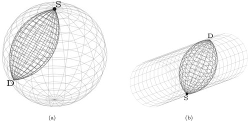
In the second modality, called here CSI${}_2$, the set of detectors are uniformly distributed on a cylinder also passing through S. Like above S could be placed inside the cylinder. The set $\mathbb{V}$ can here be represented by the vector $\mathbf{v}=\left\{R\left(\begin{array}{c}\rho \\ \cos \varphi \\ (1-\sin \varphi )\end{array}\right),\rho \in [-2,2],\varphi \in [0,2\pi ]\right\}$ with R the radius of the cylinder and S the origin of the Euclidean basis.

The object has to be placed strictly inside the sphere (respectively, the cylinder) and shall be centred to maximize the quantity of information in the data. The advantage of these approaches is to decrease the acquisition time by avoiding the rotation of the source.

However, incomplete data issues shall occur due to energetic resolution of the detector and due to non-closedness of set $\mathbb{V}$ depending on the architecture of the CSI scanner.

• The modality CSI${}_1$ is subject only to the issue on energetic resolution. Indeed, the size of the torus will increase too fast as the scattering energy/angle decrease. Its size can be symbolized by the distance between the equator of the torus and the segment SD symbolized by the segment OH on Figure 4 and given as the function $d\left(\omega \right)=\overline{\mathrm{S}\mathrm{D}}\left(\frac{1}{\sin \omega }-\frac{1}{\tan \omega }\right).$Its derivative is depicted in Figure 6 for $\overline{\mathrm{S}\mathrm{D}}=1$. The behaviour of $d^{\mathrm{\prime }}\left(\omega \right)$ shows roughly the evolution of the sampling of the tori as the scattering angle increases (resp., as the detected scattering energy decreases). This means that for given energy or angular resolution, the distance between two successive tori will be much larger for low energies than for high energies. Therefore, the information encoded in the data for low energies or high scattering angles may be irrelevant due to a lack of accuracy of the detector; one can speak of the inconsistency of the back-scattered part in the CSI data. Consequently, the sampling is inconsistent between low and high energies leading to artifacts in analytical reconstruction methods. This part of the data brings less information and can lead to artifacts in the reconstruction when using filtered backprojection type techniques. A solution could also consist in considering a nonlinear sampling for the energy in order to compensate this phenomenon, but this would lead to energetic resolution much too high to be technologically achievable. To avoid confusion, we include this phenomenon to the class of incompleteness considered here.

• In the case of the modality CSI${}_2$, the shape of the cylinder brings limited angle issues in addition to the ones seen above. Indeed, the cylinder would require an infinite length in order to get the full measurement. This is unrealistic and this is why the data in CSI${}_2$ will suffer from incomplete data, including limited angle issues.

Instead of a cylinder or a sphere, $\mathbb{V}$ could also be made for example of detector planes to facilitate the examination of large objects or for the sake of detector conception. Without a loss of generality, any surface could be considered in the choice of $\mathbb{V}$.

Figure 6. $d^{\mathrm{\prime }}\left(\omega \right)$ for $\overline{\mathrm{S}\mathrm{D}}=1$.

4. A modified multiplicative Kaczmarz algorithm for 3D CSI

When one wishes to solve an inverse problem $Ax=y\in {\mathbb{R}}^n$ as an optimization problem, the EM (expectation maximum-likelihood) algorithm searches for maximizing the likelihood functional $\sum _{i=1}^n\left(y_i\log (Ax{)}_i-(Ax{)}_i\right).$ The existence of a maximizer x is certain if and only if the Kuhn–Tucker conditions are satisfied [39]. The gradient of the likelihood leads then to the EM algorithm $x^{k+1}=x^k{A}^T\frac{y}{A{x}^k},k=0,1,\dots .$ We refer to [40,41] for standard works on the convergence and applications in imaging. The EM algorithm is notoriously slow to converge. To circumvent this issue, the ordered subset EM (OSEM) splits A and y into submatrices $A_j$ and subvectors $y_j$, $j=1,\dots ,n_p$. This approach was proposed by Hudson and Larkin [42] and can be understood as a multiplicative version of the Karzmarz method for the solution Ax = y.

In this part, we propose an iterative reconstruction method based on the OSEM algorithm, to solve the inverse problem ${\mathcal{T}}_w{n}_e=g$ under the discrete form $T_w\overline{n_e}=\overline{g}$. Section 2 models the measurement process in CSI as a linear system of equations with $T_w=\left(\begin{array}{c}{T}_{w,1}\\ ⋮\\ T_{w,P}\end{array}\right),\overline{g}=\left(\begin{array}{c}{g}_1\\ ⋮\\ g_P\end{array}\right),\overline{n_e}=\left(\begin{array}{c}{n}_1\\ ⋮\\ n_N\end{array}\right)$ with P the number of detector positions and N the number of voxels representing the electron density. The matrix $T_w$ is called the projection matrix and is split into submatrices $T_{w,j}:{\mathbb{R}}^Q\times {\mathbb{R}}^N\to {\mathbb{R}}^P$ with Q the total number of detected energies. The data $g_j\in {\mathbb{R}}^Q$ with $j=1,\dots ,P$ stands then for the data for a given detector position j and is a function of the energy $E_{\omega }$. The detected energies are equally sampled and represented by the vector $E=\left(\begin{array}{c}{E}_1\\ ⋮\\ E_Q\end{array}\right).$ The corresponding scattering angles are noted ${\omega }_k$ with $k=1,\dots ,Q$.

4.1. Computation of the projection matrix

The entries of the projection matrix are computed as the weighted toric Radon transform of a corresponding basis function with centroids noted ${\mathbf{x}}_i,i=1,\dots ,N$. Rectangular pulses (voxels) are often a standard choice to sample the 3D Euclidean space. Instead, we consider a smoother basis function with ${\delta }_i\left(\mathbf{x}\right)=\exp \left(-\frac{\parallel \mathbf{x}-{\mathbf{x}}_i\parallel }{2{\gamma }^2}\right)$ with γ a given constant, i.e. $n_e\left(\mathbf{x}\right)\approx \sum _{i=1}^N{n}_i{\delta }_i\left(\mathbf{x}\right).$ Therefore, $T_{w,j}(k,i)={\int }_{\mathrm{\Omega }}w(\mathbf{x},{\omega }_k,{\mathbf{v}}_j){\delta }_i\left(\mathbf{x}\right)\delta ({\omega }_k-\phi (\mathbf{x},{\mathbf{v}}_j,\mathbf{s}\left)\right)\mathrm{d}\mathbf{x}.$ In order to save computation time, we can assume that the weight function w varies slowly in the neighbourhood of each points ${\mathbf{x}}_i$ and get using the previous section $\begin{array}{rl}{T}_{w,j}(k,i)& \approx w(\mathbf{x},{\omega }_k,{\mathbf{v}}_j){\int }_{\mathrm{\Omega }}{\delta }_i\left(\mathbf{x}\right)\delta ({\omega }_k-\phi (\mathbf{x},{\mathbf{v}}_j,\mathbf{s}\left)\right)\mathrm{d}\mathbf{x}\\ & \approx w(\mathbf{x},{\omega }_k,{\mathbf{v}}_j){\int }_0^{2\pi }{\int }_{\pi /2-{\omega }_k}^{\pi /2+{\omega }_k}{\delta }_i\left(\mathbf{s}+\frac{\parallel {\mathbf{v}}_j\parallel }{2\sin {\omega }_k}{R}_{{\mathbf{v}}_j}\mathbf{u}(\alpha ,\text{β})\right)\\ & \times \frac{\parallel {\mathbf{v}}_j{\parallel }^2}{4{\sin }^2{\omega }_k}|\sin \alpha -\cos {\omega }_k|\mathrm{d}\alpha \mathrm{d}\text{β}.\end{array}$ Since the voxel basis $\left\{{\delta }_i\right\}$ is essentially local (a different basis could be selected to ensure the locality and the smoothness such as bump functions), the computation of the integral can be tremendously reduced by computing the angles ${\alpha }_{i,j,k},{\text{β}}_{i,j,k}$ such that ${\mathbf{x}}_i=\mathbf{s}+\frac{\parallel {\mathbf{v}}_j\parallel }{2\sin {\omega }_k}{R}_{{\mathbf{v}}_j}\mathbf{u}({\alpha }_{i,j,k},{\text{β}}_{i,j,k}),$ and then by integrating over a small neighbourhood of the pair $({\alpha }_{i,j,k},{\text{β}}_{i,j,k})$.

4.2. Poisson noise

In order to model the statistical nature of the emission and scattering of photons, we consider a Poisson process. This noise is characteristic for the emission of an ionizing source and of scattering. It is characterized by the Poisson distribution $\mathrm{P}\mathrm{r}(x=k)=\frac{{\lambda }^k}{k!}{e}^{-\lambda }$ with λ the average number of events per interval. Thus, when we consider noisy data, $\overline{g}$ will be replaced by $g^{ϵ}$ where the values $g_{jk}^{ϵ}$ are drawn following the Poisson distribution with $\lambda =g_{jk}$.

For the simulations, we have considered two phantoms: one with low contrast and for which the noise level is set to 0.5%; and one with high contrast and for which the noise level is set to 5%. To calibrate the level of noise, we tune the quantity of photons emitted by the source, noted previously $I_0$, to $\sim {10}^9$ photons in the first scenario and $\sim {10}^7$ photons in the second scenario. The error is a posteriori computed following the mean absolute error and are chosen accordingly with the contrast of each test images.

4.3. Reconstruction algorithm

The EM algorithm (Expectation–Maximization) is known to be particularly suited to deal with data corrupted by Poisson noise. This is why we focus on this approach. More precisely, we consider the ordered-subset EM algorithm (OSEM) which accelerates considerably the convergence of the EM algorithm.

However, we cannot apply strictly these algorithms given that the attenuation map remains partially unknown as pointed out in the Introduction. We propose the following adaptation of the OSEM algorithm to our case.

In the algorithm, L stands for the number of loops, $rand(1,\dots ,P)$ draws without replacement a number from 1 to P randomly following a uniform distribution, $f^{0,0}$ and $w^0$ are the initial ‘prior’ conditions. The lack of knowledge of the weight function w comes actually down to the one of the attenuation map ${\mu }_{\omega }$ since w is a function of the attenuation map. From Stonestrom et al. [43], the attenuation map is written as ${\mu }_{\omega }\left(\mathbf{x}\right)=E_{\omega }^{-3}{\mu }_{pe}\left(\mathbf{x}\right)+{\sigma }_c\left(E_{\omega }\right)n_e\left(\mathbf{x}\right)$ with ${\sigma }_c\left(E\right)$ the Klein–Nishina function [38] and ${\mu }_{PE}$ a characteristic map of the attenuating medium and $n_e$ the electron density map. The first part describes the effect of photoelectric absorption, whereas the second one gives the attenuation due to Compton scattering. The total cross-section is ${\sigma }^c=\frac{3{\sigma }_0}{4}\left(\frac{2(1+ϵ{)}^2}{{ϵ}^2(1+2ϵ)}+\frac{\ln (1+2ϵ)}{ϵ}\left(\frac{1}{2}-\frac{1+ϵ}{{ϵ}^2}\right)-\frac{1+3ϵ}{(1+2ϵ{)}^2}\right),$ with $ϵ=E_{\omega }/m{c}^2$, ${\sigma }_0=8\pi r_e^2/3$ the cross-section of the Thomson scattering, and $r_e=e^2/m_e{c}^2=2.818\times {10}^{-13}$ cm the classical electron radius. In this paper, we consider two types of applications with different energy $E_0$.

• With a low energy $E_0$ in order to limit the scattering of order higher than 2. In this case, the photoelectric absorption becomes dominant and ${\mu }_{\omega }\left(\mathbf{x}\right)\approx E_{\omega }^{-3}{\mu }_{pe}\left(\mathbf{x}\right)$. Then, the update of $w^l$ in the reconstruction algorithm can be performed via a segmentation of $f^{l+1}$, for instance K-means, assuming we know the kind of materials in the object, i.e. we know the potential values in ${\mu }_{pe}$. Such an assumption is not really restrictive in practice.

• With a high energy $E_0$ but a thin object also in order to limitate the scattering of order higher than 2. In this case, the Compton effect is dominant and thus ${\mu }_{\omega }\left(\mathbf{x}\right)\approx {\sigma }_c\left(E_{\omega }\right)n_e\left(\mathbf{x}\right)$. Then, the update of $w^l$ consists in computing ${\mu }_{\omega }^l\left(\mathbf{x}\right)={\sigma }_c\left(E_{{\omega }^l}\right)f^{l+1}\left(\mathbf{x}\right)$.

In the next section, we will see that the proposed OSEM algorithm provides satisfactory results and remains stable with Poisson noise. However, the algorithm does not denoise the reconstructed image. For this purpose, we add at the end of the algorithm a denoising step based on total variation. A standard method, see [44], consists in finding a minimizer $f^{†}$ of the functional $J\left(f\right)=\frac{1}{2}\parallel f-f^n{\parallel }_{L_2\left(\mathrm{\Omega }\right)}^2+\lambda \parallel \left|\mathrm{\nabla }f\right|{\parallel }_{L_1\left(\mathrm{\Omega }\right)}$ with $f^n$ the noisy 3D image, λ a regularization parameter and Ω the compact domain of the 3D object under study. The construction of the minimizer can be expressed as the following gradient descent flow: $\frac{\mathrm{d}f}{\mathrm{d}t}=(f^n-f)+\lambda \cdot \mathrm{d}\mathrm{i}\mathrm{v}\left(\frac{\mathrm{\nabla }f}{ϵ+|\mathrm{\nabla }f|}\right),$ where the parameter ε apodizes the singularity when $|\mathrm{\nabla }f|=0$. For the simulation results, we computed 1000 steps with $\mathrm{d}t=0.1$, $\lambda =0.5$ and $ϵ=0.1$.

A proof of the convergence of the proposed algorithm remains a mathematical challenge. The reconstruction technique as well as the measurement process in 3D CSI is illustrated in the next section via various architectures in 3D CSI and simulation results.

5. Simulation results

We consider two phantoms with specific setup and for both modalities proposed above, see Figures 7 and 8.

Figure 7. Industrial toy object. First row: central slices of $n_e\left(\mathbf{x}\right)/(6.68\times {10}^{-23})$. Second row: central slices of the prior attenuation map used to initialize the projection matrix in cm${}^{-1}$.

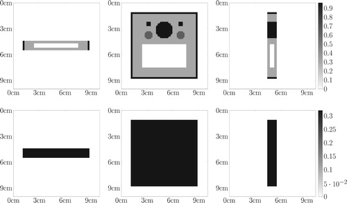
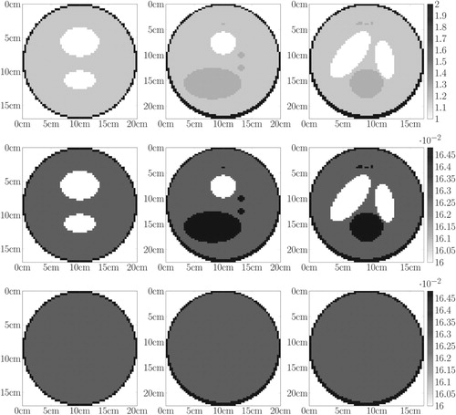
Figure 8. Medical toy object. First row: central slices of $n_e\left(\mathbf{x}\right)/(3.34\times {10}^{-23})$. Second row: central slices of the exact attenuation map in cm${}^{-1}$. Third row: central slices of the prior attenuation map in cm${}^{-1}$ used to initialize the projection matrix.

With the first phantom, we intend to illustrate industrial applications (non-destructive testing). In order to favour the scattering, the source emits with energy of 662 keV, is monochromatic and isotropic. It could correspond to the Cs-137 source. As explained in the Introduction, the toy object is flat with dimensions: $1\mathrm{c}\mathrm{m}\times 8\mathrm{c}\mathrm{m}\times 8\mathrm{c}\mathrm{m}$. A cavity is located inside as well as cylinders of different sizes. The attenuation coefficients ${\mu }_{662}\left(\mathbf{x}\right)$ are

• 0.32 cm${}^{-1}$ for the main material,

• 0.64 cm${}^{-1}$ for the two medium cylinders and

• 0.96 cm${}^{-1}$ for the others cylinders and the borders.

The electron densities are scaled according to the formula ${\mu }_E\left(\mathbf{x}\right)\approx {\sigma }_c\left(E\right)n_e\left(\mathbf{x}\right)$ evaluated in E = 662 keV. Due to the high energy $E_0$, the photoelectric absorption is neglected. The outside support is assumed to be known and is used as prior attenuation map.

With the second phantom, we intend to illustrate medical applications. In this case, the source is monochromatic and isotropic and emits with an energy of 140 keV in order to limitate multiple scattering. This could correspond to the widely used Tc99m with 98.6% of its emitted photons having energy 140 keV. The toy object is composed of spheres and ellipsoids and represents the well-known Shepp–Logan phantom in 3D. The dimensions of the main ellipsoid are $22.5\mathrm{c}\mathrm{m}\times 20\mathrm{c}\mathrm{m}\times 17\mathrm{c}\mathrm{m}$. The electron densities are obtained by multiplying the modified Shepp–Logan intensities by $3.34\times {10}^{-23}{\mathrm{c}\mathrm{m}}^{-3}$ and the attenuation coefficients ${\mu }_{140}\left(\mathbf{x}\right)$ are obtained by $0.16(1+\mathrm{S}\mathrm{L}){\mathrm{c}\mathrm{m}}^{-1}$ on the support of the object, in which $\mathrm{S}\mathrm{L}$ is the intensity map for the 3D modified Shepp–Logan. The support of the Shepp–Logan with the border part are assumed known and are used as the prior attenuation map.

5.1. Simulation results for the CSI${}_1$

This paragraph describes the simulation results for both phantoms and for the modality CSI${}_1$. The sphere is composed of 12800 ‘point’ spectral occupying $1\times 1{\mathrm{m}\mathrm{m}}^2$ regions.

• For the board phantom, we have the following parameters:

  	-	The radius of the sphere is D = 20 cm.
  	-	The source emits at 662 keV.
  	-	The energy resolution of the cameras (sampling step of the vector E) is 4.8 keV.
  	-	Also, we consider a Poisson noise of 5% (mean absolute error).
  	-	The resolution of the final image is 1 mm.

• For the Shepp–Logan phantom, we have the following parameters:

  	-	The radius of the sphere is D = 50 cm.
  	-	The source emits at 140 keV.
  	-	The energy resolution of the cameras (sampling step of the vector E) is 0.3 keV.
  	-	Also, we consider a Poisson noise of 0.5% (mean absolute error). The noise has to be low in this case as the contrast of the object is very low.
  	-	The resolution of the final image is 2.5 mm.

The 3D-CSI${}_1$ data are depicted in Figure 9. Due to the energy resolution, a part of the measurement (back-scattering) is inconsistent. As mentioned in the Introduction, the contour-based reconstruction technique proposed in [37] leads to streaks artifacts for incomplete data. This is illustrated in Figure 10. We can note that the artifacts are important and hinder the detection of the contours.

Figure 9. 3D CSI${}_1$ Data – First row depicts the data for the board phantom: (first column) 3D visualization via parallel slices, (columns 2,3,4) corresponding parallel slices. Second row depicts the data for the Shepp–Logan phantom: (first column) 3D visualization via parallel slices, (columns 2,3,4) corresponding parallel slices The greyscale (colourbar) indicates the number of detected photons, the more, the darker.

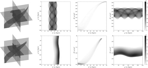
Figure 10. Central slices of the 3D contour reconstruction for the board phantom: first row – with full data, second row – with incomplete data. The intensities are rescaled dividing by $(6.68\times {10}^{-23})$.

We now apply our algorithm to the board phantom and to the Shepp–Logan phantom. The central slices of the reconstructions after one sweep for the board and after three sweeps for the Shepp–Logan phantom are, respectively, depicted on Figures 11 and 12. Figure 11 shows on the first row, the reconstruction obtained from the algorithm and on the second row, the same reconstruction after a TV-denoising step. The contrast and complexity of the Shepp–Logan phantom require less noise and more iterations to deliver a satisfactory reconstruction as depicted by Figure 12. More generally, we observe the proposed algorithm succeeds to provide a reconstruction without artifacts in spite of the incompleteness of the data and remains robust to handle the complexity of the Poisson noise (as expected from the OSEM).

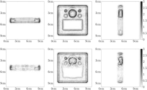
Figure 11. Central slices of the 3D reconstruction $f^{LP}$ for the board phantom: first row – before the TV-denoising step, second row – after the TV-denoising step. The intensities are rescaled dividing by $(6.68\times {10}^{-23})$.

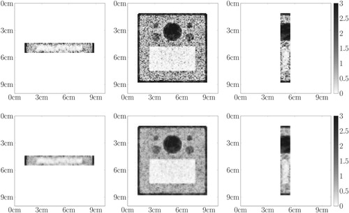
Figure 12. Central slices of the 3D reconstruction $f^{LP}$ for the Shepp–Logan phantom: first row – first iteration of the modified OSEM algorithm after the TV-denoising step, second row – third iteration of the modified OSEM algorithm after the TV-denoising step. The intensities are rescaled dividing by $(3.34\times {10}^{-23})$.

5.2. Simulation results for the CSI${}_2$

This paragraph describes the simulation results for both phantoms and for the modality CSI${}_2$. The cylinder is composed of 25600 ‘point’ spectral cameras occupying $1\times 1{\mathrm{m}\mathrm{m}}^2$ regions.

• For the board phantom, we have the following parameters:

  	-	The radius of the cylinder is R = 20 cm.
  	-	The source emits at 662 keV.
  	-	The energy resolution of the cameras (sampling step of the vector E) is 2.4 keV.
  	-	Also, we consider a Poisson noise of 5%.
  	-	The resolution of the final image is 1 mm.

• For the Shepp–Logan phantom, we have the following parameters:

  	-	The radius of the cylinder is R = 50 cm.
  	-	The source emits at 140 keV.
  	-	The energy resolution of the cameras (sampling step of the vector E) is 0.3 keV.
  	-	Also, we consider a Poisson noise of 0.5%. The noise has to be low in this case as the contrast of the object is very low.
  	-	The resolution of the final image is 2.5 mm.

The 3D-CSI${}_2$ data are depicted in Figure 13. One can observe the limited data on the third column. The data are cut or missing due to the limited energy resolution of the spectral camera and to the finite size of the cylinder. The 3D reconstructions are represented in Figures 14 and  15 via the central slices. The analysis for CSI${}_1$ still holds for the data on CSI${}_2$. One can remark that in this case the part of missing data is more important than for the previous simulations on CSI${}_1$ which explained why one needs more sweeps of the algorithm to obtain satisfactory reconstructions, respectively, five sweeps for the board phantom and three sweeps for the Shepp–Logan phantom.

Figure 13. 3D CSI${}_2$ Data – First row depicts the data for the board phantom: (first column) 3D visualization via parallel slices, (columns 2,3,4) corresponding parallel slices. Second row depicts the data for the Shepp–Logan phantom: (first column) 3D visualization via parallel slices, (columns 2,3,4) corresponding parallel slices The greyscale (colourbar) indicates the number of detected photons, the more, the darker.

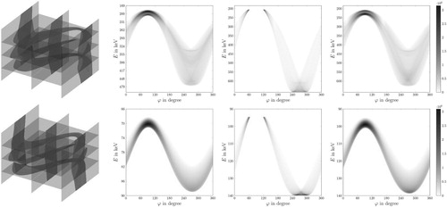
Figure 14. Central slices of the 3D reconstruction $f^{LP}$ for the board phantom: first row – first iteration of the modified OSEM algorithm before the TV-denoising step, second row – fifth iteration of the modified OSEM algorithm before the TV-denoising step, third row – fifth iteration of the modified OSEM algorithm after the TV-denoising step. The intensities are rescaled dividing by $(6.68\times {10}^{-23})$.

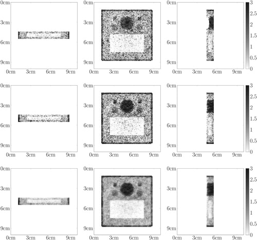
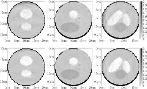
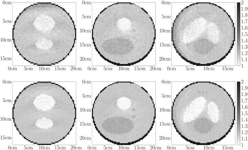
Figure 15. Central slices of the 3D reconstruction $f^{LP}$ for the Shepp–Logan phantom: first row – first iteration of the modified OSEM algorithm after the TV-denoising step, second row – third iteration of the modified OSEM algorithm after the TV-denoising step. The intensities are rescaled dividing by $(3.34\times {10}^{-23})$.

6. Discussion

In this section, we address two important aspects that have been neglected until now, namely the multiple scattering and the photoelectric absorption.

• The multiple scattering corresponds to the photons that are scattered more than once and represents a substantial part of the measured spectrum, around 50%. In [45], the author studied the impact of the second scattering and showed that the second scattering has a smoother contribution than the first scattering within the spectrum. Due to its smoothness, the variations of the multiple scattering turn out to be very low. Therefore, a reasonable a priori of the object is sufficient to compute and compensate for the multiple scattering.

• As discussed before, the attenuation can be expressed as the sum of the photoelectric absorption and the Compton scattering contribution, ${\mu }_{\omega }\left(\mathbf{x}\right)=E_{\omega }^{-3}{\mu }_{pe}\left(\mathbf{x}\right)+{\sigma }_c\left(E_{\omega }\right)n_e\left(\mathbf{x}\right).$In order to simplify, the modelling and the algorithm, we neglected the first term. Although such an assumption is reasonable for high energies and soft materials, the photoelectric absorption is not negligible for low energies (for instance in the case $E_0=140$ keV in our simulations above). However, one can proceed as in [46], i.e. use clustering techniques (such as K-means) to segment the electron density in terms of materials at each iteration. Thereby, one can deduce an approximation of ${\mu }_{pe}$ and update adequately the attenuation coefficient used in the forward operator $T_w$. More generally, since the outside isosurface of the object can be deduced from the spectral data using support theorems, the support of the object can be used to initialize the algorithm. Also, corresponding CT-scans could be used to initialize the algorithm if the type of application implies existing large databases.

We would also like to emphasize that additional considerations such as the detector material efficiency varying with the energy or detector response are not considered here but could be inserted in the forward model using a corresponding operator. Otherwise, considering a more realistic model for the camera could be treated as model uncertainty. The latter will be the focus of future research.

7. Conclusion

Following on from [37], this paper proposes a modified OSEM algorithm to deal with incomplete data issues in 3D CSI modalities. After a description of the forward modelling and of the proposed reconstruction algorithm, simulation results were proposed and applied on data corrupted with Poisson noise. The results are convincing and succeed to provide a satisfactory reconstruction after few numbers of iterations (maximum of 5 iterations), in particular giving the considered modalities have the massive advantage to require no rotation of source or object in comparison with other imaging modalities. Part of future works is to prove the convergence of the proposed algorithm and to test the algorithm on real data or at least on ground truth data obtained, for instance, by Monte-Carlo simulations.

Disclosure statement

No potential conflict of interest was reported by the author(s).

Additional information

Funding

This work was supported by the Deutsche Forschungsgemeinschaft (DFG) under the grants RI 2772/2-1 and HA 8176/1-1.

References

- Hounsfield GN. Computerized transverse axial scanning (tomography). I. Description of system. Br J Radiol. 1973;46:1016–1022. doi: 10.1259/0007-1285-46-552-1016
- Alvarez RE , Macovski A. Energy-selective reconstructions in X-ray computerized tomography. Phys Med Biol. 1976;21:733–744. doi: 10.1088/0031-9155/21/5/002
- Primak AN , Ramirez Giraldo JC , Liu X , et al. Improved dual-energy material discrimination for dual-source CT by means of additional spectral filtration. Med Phys. 2009;36:1359–1369. doi: 10.1118/1.3083567
- Shefer E , Altman A , Behling R , et al. State of the art of CT detectors and sources: a literature review. Curr Radiol Rep. 2013;1:76–91. doi: 10.1007/s40134-012-0006-4
- Tracey B , Miller E. Stabilizing dual-energy X-ray computed tomography reconstructions using patch-based regularization. Inverse Probl. 2015;31:05004. doi: 10.1088/0266-5611/31/10/105004
- McCollough CH , Leng S , Lifeng Y , et al. Dual- and multi-energy CT: principles, technical approaches, and clinical applications. Radiology. 2015;276:637–653. doi: 10.1148/radiol.2015142631
- Goo HW , Goo JM. Dual-Energy CT: new Horizon in medical imaging. Korean J Radiol. 2017;18:555–569. doi: 10.3348/kjr.2017.18.4.555
- Fredenberg E. Spectral and dual-energy X-ray imaging for medical applications. Nucl Instrum Methods Phys Res Sect A. 2018;878:74–87. doi: 10.1016/j.nima.2017.07.044
- Griesmer JJ , Kline B , Grosholz J , et al. Performance evaluation of a new CZT detector for nuclear medicine: solstice. Proceedings of the 2001 IEEE Nuclear Science Symposium Conference Record, Vol. 2; San Diego, CA, USA. IEEE; 2001. p. 1050–1054.
- Qiang L , Beilicke M , Lee K , et al. Study of thick CZT detectors for X-ray and gamma-ray astronomy. Astropart Phys. 2011;34:769–777. doi: 10.1016/j.astropartphys.2011.01.013
- Watanabe S , Ishikawa S , Aono H , et al. High energy resolution hard X-ray and gamma-ray imagers using CdTe diode devices. IEEE Trans Nucl Sci. 2009;56:777–782. doi: 10.1109/TNS.2008.2008806
- Campbell DL , Hull EL , Peterson TE. Evaluation of a compact, general-purpose Germanium Gamma camera. Proceedings of the 2013 IEEE Nuclear Science Symposium and Medical Imaging Conference; Seoul. IEEE; 2013. p. 1–6.
- Kishimoto A , Kataoka J , Koide A , et al. Development of a compact scintillator-based high-resolution Compton camera for molecular imaging. Nucl Instrum Methods Phys Res Sect A. 2017;845:656–659. doi: 10.1016/j.nima.2016.06.056
- Cherry SR , Sorenson J , Phelps M. Physics in nuclear medicine. Philadelphia : Elsevier Inc.; 2012; Available from: https://doi.org/10.1016/C2009-0-51635-2 .
- Compton AH. A quantum theory of the scattering of X-rays by light elements. Phys. Rev. 1923;21:483–502. doi: 10.1103/PhysRev.21.483
- Gibbons JP. Khan's the physics of radiation therapy. Philadelphia : Lippincott Williams & Wilkins (LWW); 2019.
- Lale PG. The examination of internal tissues, using gamma-ray scatter with a possible extension to megavoltage radiography. Phys Med Biol. 1959;4:159–167. doi: 10.1088/0031-9155/4/2/305
- Norton SJ. Compton scattering tomography. J Appl Phys. 1994;76:2007–2015. doi: 10.1063/1.357668
- Cesareo R , Cappio Borlino C , Brunetti A , et al. A simple scanner for Compton tomography. Nucl Instrum Methods Phys Res A. 2002;487:188–192. doi: 10.1016/S0168-9002(02)00964-6
- Adejumo OO , Balogun FA , Egbedokun GGO. Developing a Compton scattering tomography system for soil studies: theory. J Sustainable Dev Environ Prot. 2011;1:73–81.
- Anghaie S , Humphries LL , Diaz NJ. Material characterization and flaw detection, sizing, and location by the differential gamma scattering spectroscopy technique. part 1: development of theoretical basis. Nucl Technol. 1990;91:361–375. doi: 10.13182/NT90-A34457
- Balogun FA , Cruvinel PE. Compton scattering tomography in soil compaction study. Nucl Instrum Methods Phys Res A. 2003;505:502–507. doi: 10.1016/S0168-9002(03)01133-1
- Brunetti A , Cesareo R , Golosio B , et al. Cork quality estimation by using Compton tomography. Nucl Instrum Methods Phys Res B. 2002;196:161–168. doi: 10.1016/S0168-583X(02)01289-2
- Clarke RL , Van Dyk G. A new method for measurement of bone mineral content using both transmitted and scattered beams of gamma-rays. Phys Med Biol. 1973;18:532–539. doi: 10.1088/0031-9155/18/4/005
- Evans BL , Martin JB , Burggraf LW , et al. Nondestructive inspection using Compton scatter tomography. IEEE Trans Nucl Sci. 1998;45:950–956. doi: 10.1109/23.682682
- Farmer FT , Collins MP. A new approach to the determination of anatomical cross-sections of the body by Compton scattering of gamma-rays. Phys Med Biol. 1971;16:577–586. doi: 10.1088/0031-9155/16/4/001
- Gorshkov VA , Kroening M , Anosov YV , et al. X-Ray scattering tomography. Nondestr Test Eval. 2005;20:147–157. doi: 10.1080/10589750500191026
- Harding G , Harding E. Compton scatter imaging: a tool for historical exploitation. Appl Radiat Isot. 2010;68:993–1005. doi: 10.1016/j.apradiso.2010.01.035
- Meneley DA , Hussein EMA , Banerjee S. On the solution of the inverse problem of radiation scattering imaging. Nucl Sci Eng. 1986;92:341–349. doi: 10.13182/NSE86-A17524
- Arendtsz NV , Hussein EMA. Energy-spectral Compton scatter imaging – part 1: theory and mathematics. IEEE Trans Nucl Sci. 1995;42:2155–2165. doi: 10.1109/23.489441
- Guzzardi R , Licitra G. A critical review of Compton imaging. CRC Crit Rev Biomed Imaging. 1988;15:237–268.
- Rigaud G. Compton scattering tomography: feature reconstruction and rotation-free modality. SIAM J Imaging Sci. 2017;10:2217–2249. doi: 10.1137/17M1120105
- Redler G , Jones KC , Templeton A , et al. Compton scatter imaging: a promising modality for image guidance in lung stereotactic body radiation therapy. Med Phys. 2018;45:1233–1240. doi: 10.1002/mp.12755
- Jones KC , Redler G , Templeton A , et al. Characterization of Compton-scatter imaging with an analytical simulation method. Phys Med Biol. 2018;63:025016.
- Nguyen MK , Truong TT , Morvidone M , et al. Scattered radiation emission imaging: principles and applications. Int J Biomed Imaging. 2011;2011:913893. doi: 10.1155/2011/913893
- Prado PG , Nguyen MK , Dumas L , et al. Three-dimensional imaging of flat natural and cultural heritage objects by a Compton scattering modality. J Electron Imaging. 2017;26:011026.
- Rigaud G , Hahn B. 3D Compton scattering imaging and contour reconstruction for a class of Radon transforms. Inverse Probl. 2018;34:075004. doi: 10.1088/1361-6420/aabf0b
- Klein I , Nishina Y. Über die streuung von strahlung durch freie elektronen nach der neuen relativistischen quantendynamik von dirac. Z Phys. 1929;52:853–869. doi: 10.1007/BF01366453
- Kuhn HW , Tucker AW. Nonlinear programming. In: Neyman J, editor. Proceedings of the 2nd Berkeley Symposium on Mathematical Statistics and Probability. Berkeley, CA: University of California Press; 1951. p. 481–492.
- Shepp LA , Vardi Y. Maximum likelihood reconstruction for emission tomography. IEEE Trans Med Imaging. 1982;1:113–122. doi: 10.1109/TMI.1982.4307558
- Vardi Y , Shepp LA , Kaufman L. A statistical model for positron emission tomography. J Amer Stat Assoc. 1985;80:8–20. doi: 10.1080/01621459.1985.10477119
- Hudson HM , Larkin RS. Accelerated EM reconstruction using ordered subsets of projection data. IEEE Trans Med Imaging. 1994;13:601–609. doi: 10.1109/42.363108
- Stonestrom JP , Alvarez RE , Macovski A. A framework for spectral artifact corrections in X-ray CT. IEEE Trans Biomed Eng. 1981;28:128–141. doi: 10.1109/TBME.1981.324786
- Rudin LI , Osher S , Fatemi E. Nonlinear total variation based noise removal algorithms. Physica D. 1992;60:259–268. doi: 10.1016/0167-2789(92)90242-F
- Rigaud G. 3D Compton scattering imaging: study of the spectrum and contour reconstruction; 2019. arXiv:1908.03066.
- Rigaud G , Régnier R , Nguyen MK , et al. Combined modalities of Compton scattering tomography. IEEE Trans Nucl Sci. 2013;60:1570–1577. doi: 10.1109/TNS.2013.2252022