Recovering space-dependent source for a time-space fractional diffusion wave equation by fractional Landweber method

Abstract

In this paper, we consider a problem of recovering a space-dependent source for a time fractional diffusion wave equation by the fractional Landweber method. The inverse problem has been transformed into an integral equation by using the final measured data. We use the fractional Landweber regularization method for overcoming the ill-posedness. We discuss an a-priori regularization parameter choice rule and an a-posteriori regularization parameter choice rule, and we also prove the conditional stability and convergence rates for the inverse problem. Numerical experiments for four examples in one-dimensional and two-dimensional cases are provided to show the effectiveness of the proposed method.

Keywords:

• Fractional diffusion wave equation
• inverse problem
• fractional Landweber method
• convergence estimates
• numerical calculation

2010 Mathematics Subject Classification:

• Inverse Problem

1. Introduction

Let Ω be a bounded domain in ${\mathbb{R}}^d$ with sufficiently smooth boundary $\mathrm{\partial }\mathrm{\Omega }$. Suppose $d\le 3$, consider the following time-space fractional diffusion wave equation: (1) $\begin{array}{rl}{\mathrm{\partial }}_{0+}^{\alpha }u(x,t)+(-\mathrm{\Delta }{)}^{\frac{\beta }{2}}u(x,t)=f(x),x& \in \mathrm{\Omega },0<t\le T,\\ u(x,0)& =a(x),x\in \mathrm{\Omega },\\ u_t(x,0)& =b(x),x\in \mathrm{\Omega },\\ u(x,t)& =0,x\in \mathrm{\partial }\mathrm{\Omega },0<t\le T,\end{array}$(1) where $\alpha \in (1,2),\beta \in (1,2)$ are fractional orders of the time and space derivatives, respectively, T>0 is a fixed-final time.

The Caputo fractional left-sided derivative of order α with respect to t defined by ${\mathrm{\partial }}_{0+}^{\alpha }u(x,t)=\frac{1}{\mathrm{\Gamma }(2-\alpha )}{\int }_0^t\frac{{\mathrm{\partial }}_{ss}u(x,s)}{(t-s{)}^{\alpha -1}}\mathrm{d}s,$ in which $\mathrm{\Gamma }(\cdot )$ is the Gamma function.

The fractional Laplacian operator $(-\mathrm{\Delta }{)}^{\beta /2}$ of order β is defined by using spectral decomposition of the Laplace operator. The definition is summarized in Definition 2.1.

Denote $g(x)=u(x,T)$ as the final time data. Since the measurement is noise-contaminated inevitably, we denote the noisy measurement of g as $g^{\delta }$ which satisfies (2) $\Vert g^{\delta }-g\Vert \le \delta ,$(2) where $\Vert \cdot \Vert$ is the $L^2(\mathrm{\Omega })$ norm throughout this paper.

In this paper, we consider the following inverse problems:

(IP:) Suppose $a(x),b(x)$ are known, we reconstruct $f(x)$ from the measurement $g^{\delta }(x)$.

The physical background for a time-space fractional diffusion wave equation can be seen in [1]. Recently, the direct problems for time-fractional diffusion wave equations have been investigated, such as [2–9]. However, as we know, the inverse problems for fractional wave equations have not been investigated widely. An inverse initial value problem [10–14], an inverse time-dependent source problem [15–18], the uniqueness of inverse coefficients [19]. An inverse space-dependent source by the Landweber method [20].

As we known, recovering the space-dependent coefficient problems have not been investigated widely in a time-fractional diffusion wave equation. We just found a few papers. Yan and Wei [21] have proved the uniqueness of inverse space-dependent source problem by the part of Dirichlet boundary data. In this paper, we provide the fractional Landweber method [11,22,23] to solve this inverse space-dependent source problem for time-space fractional diffusion equation. Since the uniqueness for inverse problem may not hold, we have to consider the approximate solution. We consider the conditional stability for the inverse problem and present the convergence rate of the fractional Landweber regularized solution approach to the approximate solution under an a priori assumption by using an a-priori parameter choice rule and an a-posteriori parameter choice rule, respectively. Four numerical examples are presented to show the efficiency of the proposed approach.

The remainder of this paper is composed of six sections. In Section 2, we present some preliminaries used in Sections 3, 4 and 5. In Section 3, we show the conditional stability of the inverse problem. In Sections 4 and 5, we propose the fractional Landweber regularization method and give two convergence estimates under an a priori assumption for exact solution and two regularization parameter choice rules. In Section 6, we test some numerical examples. Finally, we give a conclusion in Section 7.

2. Preliminary

Throughout this paper, we use the following definitions and propositions.

Definition 2.1

[24–26]

Suppose $\{{\lambda }_k,{\phi }_k\}$ be the eigenvalues and corresponding eigenvectors of the Laplacian operator $-\mathrm{\Delta }$ in Ω with Dirichlet boundary condition on $\mathrm{\partial }\mathrm{\Omega }$: (3) $\begin{array}{ll}-\mathrm{\Delta }{\phi }_k={\lambda }_k{\phi }_k,& \mathrm{in}\mathrm{\Omega },\\ {\phi }_k=0,& \mathrm{on}\mathrm{\partial }\mathrm{\Omega }.\end{array}$(3) Counting according to the multiplicities, we can assume (4) $0<{\lambda }_1\le {\lambda }_2\le \cdots \le {\lambda }_n\le \cdots ,\underset{n\to \mathrm{\infty }}{lim}{\lambda }_n=+\mathrm{\infty }.$(4) Let $H_0^{\beta }(\mathrm{\Omega }):=\{u=\sum _{n=1}^{\mathrm{\infty }}{a}_n{\phi }_n:\Vert u{\Vert }_{H_0^{\beta }(\mathrm{\Omega })}^2=\sum _{n=1}^{\mathrm{\infty }}{a}_n^2{{\lambda }_n}^{\beta }<\mathrm{\infty }\},$ we define the operator $(-\mathrm{\Delta }{)}^{\beta /2}$ by $(-\mathrm{\Delta }{)}^{\frac{\beta }{2}}u=\sum _{n=1}^{\mathrm{\infty }}{a}_n{{\lambda }_n}^{\frac{\beta }{2}}{\phi }_n,$ which maps $H_0^{\beta /2}(\mathrm{\Omega })$ onto $L^2(\mathrm{\Omega }),$ with the following equivalence: $\Vert u{\Vert }_{H_0^{\beta }}=\Vert (-\mathrm{\Delta }{)}^{\frac{\beta }{2}}u{\Vert }_{L^2(\mathrm{\Omega })}.$ Note that if α tends to 2 and β tends to 2, the fractional derivative ${\mathrm{\partial }}_{0+}^{\alpha }$ tends to the second-order derivative $u_{tt}$ and the fractional Laplacian operator $(-\mathrm{\Delta }{)}^{\beta /2}$ tends to the Laplacian operator $-\mathrm{\Delta },$ and thus model (1(1) $\begin{array}{rl}{\mathrm{\partial }}_{0+}^{\alpha }u(x,t)+(-\mathrm{\Delta }{)}^{\frac{\beta }{2}}u(x,t)=f(x),x& \in \mathrm{\Omega },0<t\le T,\\ u(x,0)& =a(x),x\in \mathrm{\Omega },\\ u_t(x,0)& =b(x),x\in \mathrm{\Omega },\\ u(x,t)& =0,x\in \mathrm{\partial }\mathrm{\Omega },0<t\le T,\end{array}$(1) ) reproduces the standard diffusion wave equation.

Definition 2.2

[27,28]

The generalized Mittag-Leffler function is defined by $E_{\alpha ,\beta }(z)=\sum _{k=0}^{\mathrm{\infty }}\frac{z^k}{\mathrm{\Gamma }(\alpha k+\beta )},z\in \mathbb{C},$ where $\alpha >0,\beta \in \mathbb{R}$.

Lemma 2.3

[12]

For $1<\alpha <2$ and $\{{\lambda }_n\}$ are given in (4(4) $0<{\lambda }_1\le {\lambda }_2\le \cdots \le {\lambda }_n\le \cdots ,\underset{n\to \mathrm{\infty }}{lim}{\lambda }_n=+\mathrm{\infty }.$(4) ), there exist positive constants $\underset{\_}{C},\overline{C}$ depending on $\alpha ,T$ and finite eigenvalues ${\lambda }_n$ such that $\frac{\underset{\_}{C}}{{\lambda }_n^{\frac{\beta }{2}}}\le |E_{\alpha ,\alpha +1}(-{\lambda }_n^{\frac{\beta }{2}}{T}^{\alpha })|\le \frac{\overline{C}}{{\lambda }_n^{\frac{\beta }{2}}},n\in \mathbb{N}.$

Lemma 2.4

For $\frac{1}{2}<\gamma <1,m\ge 1,0<\mu T^{\alpha }{E}_{\alpha ,\alpha +1}(-{\lambda }_n^{\beta /2}{T}^{\alpha })<1,$ we have $\underset{n\in \mathbb{N}}{sup}{(1-\mu T^{2\alpha }{E}_{\alpha ,\alpha +1}^2(-{\lambda }_n^{\frac{\beta }{2}}{T}^{\alpha }))}^m{(T^{\alpha }{E}_{\alpha ,\alpha +1}(-{\lambda }_n^{\frac{\beta }{2}}{T}^{\alpha }))}^p\le C(\mu ,p)m^{\frac{-p}{2}},$ where the constant $C(\mu ,p)$ is given by $C(\mu ,p)=(\frac{p}{2\mu }{)}^{p/2}$.

Proof.

We introduce a new variable $x:=T^{2\alpha }{E}_{\alpha ,\alpha +1}^2(-{\lambda }_n^{\beta /2}{T}^{\alpha })<\frac{1}{\mu }$ and define a function $q(x)=(1-\mu x{)}^m{x}^{p/2}$. It is easy to verify that there exists a unique $x_0=\frac{s}{\mu (s+m)}<\frac{1}{\mu }$ with $s=\frac{p}{2}$ such that $q^{\prime }(x_0)=0$. We then have $\begin{array}{rl}q(x)& \le q(x_0)\le {(1-\frac{s}{s+m})}^m{\left(\frac{s}{\mu (s+m)}\right)}^s<\left(\frac{s}{\mu }\right){\left(\frac{1}{s+m}\right)}^s\\ & <{\left(\frac{s}{\mu }\right)}^s{\left(\frac{1}{m}\right)}^s:=C(\mu ,p)m^{\frac{-p}{2}}.\end{array}$

Lemma 2.5

[29]

Let $K:X\to Y$ be bounded linear operator.

1. $x\in X$ is called a least-squares solution of Kx = y if $\Vert Kx-y\Vert =inf\{\Vert Kz-y\Vert |z\in X\}.$

2. $x\in X$ is called a best-approximate solution of Kx = y if x is a least-squares solution of Kx = y and $\Vert x\Vert =inf\{\Vert z\Vert |z\mathit{\text{is the least-squares solution of}}Kx=y\}$ holds.

3. The conditional stability of the inverse problem

From [2], we have the following result.

Theorem 3.1

Let $a\in H^{\beta }(\mathrm{\Omega }),b\in H^{-1}(\mathrm{\Omega })$ and $f\in L^2(\mathrm{\Omega }),$ then there exists a unique weak solution $u\in C([0,T];L^2(\mathrm{\Omega }))\cap L^2(0,T;H_0^{\beta }(\mathrm{\Omega }))$ and the solution for (1(1) $\begin{array}{rl}{\mathrm{\partial }}_{0+}^{\alpha }u(x,t)+(-\mathrm{\Delta }{)}^{\frac{\beta }{2}}u(x,t)=f(x),x& \in \mathrm{\Omega },0<t\le T,\\ u(x,0)& =a(x),x\in \mathrm{\Omega },\\ u_t(x,0)& =b(x),x\in \mathrm{\Omega },\\ u(x,t)& =0,x\in \mathrm{\partial }\mathrm{\Omega },0<t\le T,\end{array}$(1) ) is given by (5) $\begin{array}{rl}u(x,t)& =\sum _{n=1}^{\mathrm{\infty }}\{(a,{\phi }_n)E_{\alpha ,1}(-{\lambda }_n^{\frac{\beta }{2}}{t}^{\alpha })+(b,{\phi }_n)t{E}_{\alpha ,2}(-{\lambda }_n^{\frac{\beta }{2}}{t}^{\alpha })+(f,{\phi }_n)t^{\alpha }{E}_{\alpha ,\alpha +1}\\ & (-{\lambda }_n^{\frac{\beta }{2}}{t}^{\alpha })\}{\phi }_n(x),\end{array}$(5) where $(a,{\phi }_n),(b,{\phi }_n)$ and $(f,{\phi }_n)$ are the Fourier coefficients.

Proof.

The proof of this theorem is similar to the proof of Theorem 3.2 of Literature [30]

Let t = T in (5(5) $\begin{array}{rl}u(x,t)& =\sum _{n=1}^{\mathrm{\infty }}\{(a,{\phi }_n)E_{\alpha ,1}(-{\lambda }_n^{\frac{\beta }{2}}{t}^{\alpha })+(b,{\phi }_n)t{E}_{\alpha ,2}(-{\lambda }_n^{\frac{\beta }{2}}{t}^{\alpha })+(f,{\phi }_n)t^{\alpha }{E}_{\alpha ,\alpha +1}\\ & (-{\lambda }_n^{\frac{\beta }{2}}{t}^{\alpha })\}{\phi }_n(x),\end{array}$(5) ), we have $\begin{array}{rl}u(x,T)& =\sum _{n=1}^{\mathrm{\infty }}\{(a,{\phi }_n)E_{\alpha ,1}(-{\lambda }_n^{\frac{\beta }{2}}{T}^{\alpha })+(b,{\phi }_n)T{E}_{\alpha ,2}(-{\lambda }_n^{\frac{\beta }{2}}{T}^{\alpha })\\ & +(f,{\phi }_n)T^{\alpha }{E}_{\alpha ,\alpha +1}(-{\lambda }_n^{\frac{\beta }{2}}{T}^{\alpha })\}{\phi }_n(x)=g(x).\end{array}$ Denote $h(x)=\sum _{n=1}^{\mathrm{\infty }}\{(a,{\phi }_n)E_{\alpha ,1}(-{\lambda }_n^{\frac{\beta }{2}}{T}^{\alpha })+(b,{\phi }_n)T{E}_{\alpha ,2}(-{\lambda }_n^{\frac{\beta }{2}}{T}^{\alpha })\}{\phi }_n(x)$ and $J(x)=g(x)-h(x),$ then we have (6) $\sum _{n=1}^{\mathrm{\infty }}(f,{\phi }_n)T^{\alpha }{E}_{\alpha ,\alpha +1}(-{\lambda }_n^{\frac{\beta }{2}}{T}^{\alpha }){\phi }_n(x)=J(x).$(6) The inverse problem (IP) becomes the following integral equation: (7) $Kf(\xi )={\int }_{\mathrm{\Omega }}K(x,\xi )f(\xi )\mathrm{d}\xi =J(x),$(7) where the integral kernel is (8) $K(x,\xi )=\sum _{n=1}^{\mathrm{\infty }}{T}^{\alpha }{E}_{\alpha ,\alpha +1}(-{\lambda }_n^{\frac{\beta }{2}}{T}^{\alpha }){\phi }_n(x){\phi }_n(\xi ).$(8) By Theorem 3.1, we known if $f\in L^2(\mathrm{\Omega }),Kf\in H_0^{\beta }(\mathrm{\Omega })$. And due to the compact embedding into $L^2(\mathrm{\Omega }),$ we known the linear operators K are compact from $L^2(\mathrm{\Omega })$ into $L^2(\mathrm{\Omega })$. The inverse problems (IP) is ill-posed.

Let $K^{\ast }$ be the adjoint of K. Since $\{{\phi }_n{\}}_{n=1}^{\mathrm{\infty }}$ are orthonormal in $L^2(\mathrm{\Omega }),$ it is easy to verify $K^{\ast }K{\phi }_n(\xi )={\left(T^{\alpha }{E}_{\alpha ,\alpha +1}(-{\lambda }_n^{\frac{\beta }{2}}{T}^{\alpha })\right)}^2{\phi }_n(\xi ).$ Hence, the singular values of K are ${\sigma }_n^{(1)}=|T^{\alpha }{E}_{\alpha ,\alpha +1}(-{\lambda }_n^{\beta /2}{T}^{\alpha })|$. Define ${\psi }_n^{(1)}(x)=\{\begin{array}{l}{\phi }_n(x),E_{\alpha ,\alpha +1}(-{\lambda }_n^{\frac{\beta }{2}}{T}^{\alpha })\ge 0,\\ -{\phi }_n(x),E_{\alpha ,\alpha +1}(-{\lambda }_n^{\frac{\beta }{2}}{T}^{\alpha })<0.\end{array}$ It is clear that $\{{\psi }_n^{(1)}{\}}_{n=1}^{\mathrm{\infty }}$ are orthonormal in $L^2(\mathrm{\Omega }),$ we can verify (9) $\begin{array}{rl}K{\phi }_n(\xi )& ={\sigma }_n^{(1)}{\psi }_n^{(1)}(x)=T^{\alpha }{E}_{\alpha ,\alpha +1}(-{\lambda }_n^{\frac{\beta }{2}}{T}^{\alpha }){\phi }_n(x),\end{array}$(9) (10) $\begin{array}{rl}{K}^{\ast }{\psi }_n^{(1)}(x)& ={\sigma }_n^{(1)}{\phi }_n(\xi )=T^{\alpha }{E}_{\alpha ,\alpha +1}(-{\lambda }_n^{\frac{\beta }{2}}{T}^{\alpha }){\psi }_n^{(1)}(x).\end{array}$(10) Therefore, the singular system of K is $({\sigma }_n^{(1)};{\phi }_n,{\psi }_n^{(1)})$.

On the properties of the singular value, we give the following lemma.

Lemma 3.2

[12]

For $1<\alpha <2$ and any fixed $T>0,$ there is at most a finite index set $I=\{n_1,n_2,\dots ,n_N\}$ such that $E_{\alpha ,\alpha +1}(-{\lambda }_n^{\beta /2}{T}^{\alpha })=0$ for $n\in I$ and $E_{\alpha ,\alpha +1}(-{\lambda }_n^{\beta /2}{T}^{\alpha })\ne 0$ for $n\notin I$.

Remark 3.1

The index sets I may be empty, that means the singular values for the operators K are not zeros. Here and below, all the results for $I=\varnothing$ is regarded as special cases.

In the following, the integral kernels given in (8(8) $K(x,\xi )=\sum _{n=1}^{\mathrm{\infty }}{T}^{\alpha }{E}_{\alpha ,\alpha +1}(-{\lambda }_n^{\frac{\beta }{2}}{T}^{\alpha }){\phi }_n(x){\phi }_n(\xi ).$(8) ) is rewritten as (11) $K(x,\xi )=\sum _{n=1,n\notin I}^{\mathrm{\infty }}{T}^{\alpha }{E}_{\alpha ,\alpha +1}(-{\lambda }_n^{\frac{\beta }{2}}{T}^{\alpha }){\phi }_n(x){\phi }_n(\xi ).$(11) The kernel spaces of operators K is $N(K)=\mathrm{span}\{{\phi }_n;n\in I\}\mathrm{for}I\ne \varnothing ,N(K)=\{0\}\mathrm{for}I=\varnothing ,$ and the ranges of the operators K is $R(K)=\{J\in L^2(\mathrm{\Omega })|(J,{\phi }_n)=0,n\in I;\sum _{n=1,n\notin I}^{\mathrm{\infty }}{\left(\frac{(J,{\phi }_n)}{T^{\alpha }{E}_{\alpha ,\alpha +1}(-{\lambda }_n^{\frac{\beta }{2}}{T}^{\alpha })}\right)}^2<\mathrm{\infty }\}.$ Therefore, we have the following existence of the solution for the integral equation.

Theorem 3.3

If $I=\varnothing ,$ for any $J\in R(K),$ there exists a unique solution in $L^2(\mathrm{\Omega })$ for the integral Equation (7(7) $Kf(\xi )={\int }_{\mathrm{\Omega }}K(x,\xi )f(\xi )\mathrm{d}\xi =J(x),$(7) ) given by $f^{+}(x)=\sum _{n=1}^{\mathrm{\infty }}\frac{(J,{\phi }_n)}{T^{\alpha }{E}_{\alpha ,\alpha +1}(-{\lambda }_n^{\frac{\beta }{2}}{T}^{\alpha })}{\phi }_n(x).$ If $I\ne \varnothing ,$ for any $J\in R(K),$ there exist infinitely many solutions for the integral Equation (7(7) $Kf(\xi )={\int }_{\mathrm{\Omega }}K(x,\xi )f(\xi )\mathrm{d}\xi =J(x),$(7) ), but exists only one best-approximate solution in $L^2(\mathrm{\Omega })$ as (12) $f^{+}(x)=\sum _{n=1,n\notin I}^{\mathrm{\infty }}\frac{(J,{\phi }_n)}{T^{\alpha }{E}_{\alpha ,\alpha +1}(-{\lambda }_n^{\frac{\beta }{2}}{T}^{\alpha })}{\phi }_n(x).$(12)

Proof.

Suppose $f^{+}(\xi )=\sum _{n=1}^{\mathrm{\infty }}{f}_n{\phi }_n,$ putting into (7(7) $Kf(\xi )={\int }_{\mathrm{\Omega }}K(x,\xi )f(\xi )\mathrm{d}\xi =J(x),$(7) ) with $J=\sum _{n=1,n\notin I}(J,{\phi }_n){\phi }_n,$ according to the orthonormality of $\{{\phi }_n\},$ it is not hard to obtain the results.

Now, we give conditional stabilities in the following theorem.

Theorem 3.4

For any $f(x)\in H^{\beta p}\cap N(K{)}^{\perp }$ satisfying an a priori bound condition (13) $\Vert f{\Vert }_{H^{\beta p}}\le E,p>1,$(13) then we have $\Vert f\Vert \le C_3{E}^{\frac{1}{p+1}}\Vert Kf{\Vert }^{\frac{p}{p+1}},p>1,$ where $C_3=C(\alpha ,T,p)$ is positive constant.

Proof.

The proof of this theorem is similar to the proof of Theorem 3.2 of Literature [10].

4. Convergence estimate under an a priori regularization parameter choice rule

In this section, we use the fractional Landweber method to solve the inverse problem (IP) and give the fractional Landweber regularized solutions. The iterative implementation of the fractional Landweber method can be found in [22].

Denote the fractional Landweber regularization solution with the exact data by (14) $f_m(x)=\sum _{n=1,n\notin I}^{\mathrm{\infty }}\frac{{[1-{(1-\mu T^{2\alpha }{E}_{\alpha ,\alpha +1}^2(-{\lambda }_n^{\frac{\beta }{2}}{T}^{\alpha }))}^m]}^{\gamma }}{T^{\alpha }{E}_{\alpha ,\alpha +1}(-{\lambda }_n^{\frac{\beta }{2}}{T}^{\alpha })}{J}_n{\phi }_n(x),\frac{1}{2}\le \gamma \le 1,$(14) and the fractional Landweber regularization solution with the noisy data by (15) $f_m^{\delta }(x)=\sum _{n=1,n\notin I}^{\mathrm{\infty }}\frac{{[1-{(1-\mu T^{2\alpha }{E}_{\alpha ,\alpha +1}^2(-{\lambda }_n^{\frac{\beta }{2}}{T}^{\alpha }))}^m]}^{\gamma }}{T^{\alpha }{E}_{\alpha ,\alpha +1}(-{\lambda }_n^{\frac{\beta }{2}}{T}^{\alpha })}{J}_n^{\delta }{\phi }_n(x),\frac{1}{2}\le \gamma \le 1,$(15) respectively, where $J^{\delta }=g^{\delta }-\sum _{n=1}^{\mathrm{\infty }}[(a,\phi )E_{\alpha ,1}(-{\lambda }_n^{\beta /2}{T}^{\alpha })+(b,{\phi }_n)T{E}_{\alpha ,2}(-{\lambda }_n^{\beta /2}{T}^{\alpha })]{\phi }_n(x),m>0$ plays the role of regularization parameter, μ is an accelerated factor satisfying $0<\mu <\frac{1}{T^{2\alpha }{E}_{\alpha ,\alpha +1}^2(-{\lambda }_n^{\beta /2}{T}^{\alpha })},$ and γ is called the fractional parameter. When $\gamma =1,$ it is the classic Landweber iterative method.

Theorem 4.1

Let $m=\lfloor {\left(\frac{E}{\delta }\right)}^{2/(p+1)}\rfloor$. If the a priori condition (13(13) $\Vert f{\Vert }_{H^{\beta p}}\le E,p>1,$(13) ) and the noise assumption (2(2) $\Vert g^{\delta }-g\Vert \le \delta ,$(2) ) hold, we have the following convergence estimate: $\Vert f_m^{\delta }-f^{+}\Vert \le (c_1+c_2)E{}^{\frac{1}{p+1}}{\delta }^{\frac{p}{p+1}},$ where $\lfloor m\rfloor$ denotes the largest smaller than or equal to m and $c_1,c_2$ are positive constants depending on $\mu ,p,\gamma$ and $\underset{\_}{C}$.

Proof.

By the triangle inequality, we know (16) $\Vert f_m^{\delta }-f^{+}\Vert \le \Vert f_m^{\delta }-f_m\Vert +\Vert f_m-f^{+}\Vert =I_1+I_2.$(16) We need to estimate $I_1$ firstly, by (2(2) $\Vert g^{\delta }-g\Vert \le \delta ,$(2) ) we have (17) $\begin{array}{rl}{I}_1& =\Vert f_m^{\delta }-f_m\Vert \\ & =\Vert \sum _{n=1,n\notin I}^{\mathrm{\infty }}\frac{{[1-{(1-\mu T^{2\alpha }{E}_{\alpha ,\alpha +1}^2(-{\lambda }_n^{\frac{\beta }{2}}{T}^{\alpha }))}^m]}^{\gamma }}{T^{\alpha }{E}_{\alpha ,\alpha +1}(-{\lambda }_n^{\frac{\beta }{2}}{T}^{\alpha })}(J_n^{\delta }-J_n){\phi }_n(x)\Vert \\ & \le \delta \underset{n\ne I}{sup}\frac{{[1-{(1-\mu T^{2\alpha }{E}_{\alpha ,\alpha +1}^2(-{\lambda }_n^{\frac{\beta }{2}}{T}^{\alpha }))}^m]}^{\gamma }}{T^{\alpha }{E}_{\alpha ,\alpha +1}(-{\lambda }_n^{\frac{\beta }{2}}{T}^{\alpha })}.\end{array}$(17) Let ${\xi }^2=\mu T^{2\alpha }{E}_{\alpha ,\alpha +1}^2(-{\lambda }_n^{\beta /2}{T}^{\alpha })$ and $\varphi (\xi )={\xi }^{-2}[1-(1-{\xi }^2{)}^m{]}^{2\gamma }.$ Since $0<\mu <\frac{1}{T^{2\alpha }{E}_{\alpha ,\alpha +1}^2(-{\lambda }_n^{\beta /2}{T}^{\alpha })},n\notin I,$ we have $0<\mu T^{2\alpha }{E}_{\alpha ,\alpha +1}^2(-{\lambda }_n^{\beta /2}{T}^{\alpha })<1,n\notin I$. Hence, the function is continuous when $\xi \in (0,1)$.

For $\gamma \in (\frac{1}{2},1)$ and $\xi \in (0,1),$ using Lemma 3.3 in [22] $\varphi (\xi )\le m,$ then $\underset{n\ne I}{sup}{\frac{{[1-{(1-\mu T^{2\alpha }{E}_{\alpha ,\alpha +1}^2(-{\lambda }_n^{\frac{\beta }{2}}{T}^{\alpha }))}^m]}^{\gamma }}{T^{\alpha }{E}_{\alpha ,\alpha +1}(-{\lambda }_n^{\frac{\beta }{2}}{T}^{\alpha })}\le \mu }^{\frac{1}{2}}{m}^{\frac{1}{2}}.$ So we have (18) $\Vert f_m^{\delta }-f_m\Vert \le \delta {\mu }^{\frac{1}{2}}{m}^{\frac{1}{2}}.$(18) For the second item on the right-hand side of (16(16) $\Vert f_m^{\delta }-f^{+}\Vert \le \Vert f_m^{\delta }-f_m\Vert +\Vert f_m-f^{+}\Vert =I_1+I_2.$(16) ), by Proposition 3.5 in [22],

(19) $\begin{array}{rl}& \Vert f_m-f^{+}\Vert \\ & =\Vert \sum _{n\notin I}^{\mathrm{\infty }}[1-{[1-{(1-\mu T^{2\alpha }{E}_{\alpha ,\alpha +1}^2(-{\lambda }_n^{\frac{\beta }{2}}{T}^{\alpha }))}^m]}^{\gamma }]\frac{J_n}{T^{\alpha }{E}_{\alpha ,\alpha +1}(-{\lambda }_n^{\frac{\beta }{2}}{T}^{\alpha })}{\phi }_n(x)\Vert \\ & \le \Vert \sum _{n=1,n\notin I}^{\mathrm{\infty }}{(1-\mu T^{2\alpha }{E}_{\alpha ,\alpha +1}^2(-{\lambda }_n^{\frac{\beta }{2}}{T}^{\alpha }))}^m{\lambda }_n^{\frac{-\beta p}{2}}\frac{{\lambda }_n^{\frac{\beta p}{2}}{J}_n}{T^{\alpha }{E}_{\alpha ,\alpha +1}(-{\lambda }_n^{\frac{\beta }{2}}{T}^{\alpha })}{\phi }_n(x)\Vert \\ & =\Vert \sum _{n=1,n\notin I}^{\mathrm{\infty }}{(1-\mu T^{2\alpha }{E}_{\alpha ,\alpha +1}^2(-{\lambda }_n^{\frac{\beta }{2}}{T}^{\alpha }))}^m{\lambda }_n{}^{\frac{-\beta p}{2}}{\lambda }_n{}^{\frac{\beta p}{2}}{f}_n{\phi }_n(x)\Vert \\ & \le E\underset{n\notin I}{sup}{(1-\mu T^{2\alpha }{E}_{\alpha ,\alpha +1}^2(-{\lambda }_n^{\frac{\beta }{2}}{T}^{\alpha }))}^m{\lambda }_n^{\frac{-\beta p}{2}}.\end{array}$(19) Denote $S(n)={(1-\mu T^{2\alpha }{E}_{\alpha ,\alpha +1}^2(-{\lambda }_n^{\frac{\beta }{2}}{T}^{\alpha }))}^m{\lambda }_n^{\frac{-\beta p}{2}}.$ By Lemma 2.3, we get $S(n)\le {(1-\mu T^{2\alpha }{E}_{\alpha ,\alpha +1}^2(-{\lambda }_n^{\frac{\beta }{2}}{T}^{\alpha }))}^m{\left(T^{\alpha }{E}_{\alpha ,\alpha +1}(-{\lambda }_n^{\frac{\beta }{2}}{T}^{\alpha })\right)}^p.$ Let $H(s)=(1-\mu s{)}^m{s}^{\frac{p}{2}},s=T^{2\alpha }{E}_{\alpha ,\alpha +1}^2(-{\lambda }_n^{\frac{\beta }{2}}{T}^{\alpha }).$ By Lemma 2.4, we have $h(s)\le EC(\mu ,p)m^{\frac{-p}{2}}.$ Combining the above two inequalities, we obtain $\Vert f_m^{\delta }(x)-f(x)\Vert \le {\mu }^{\frac{1}{2}}{m}^{\frac{1}{2}}\delta +EC(\mu ,p)m^{\frac{-p}{2}}.$ Choosing the regularization parameter m by $m=\lfloor (\frac{E}{\delta }{)}^{2/(p+1)}\rfloor ,$ we then obtain the following convergence estimate $\Vert f_m^{\delta }(x)-f(x)\Vert \le (c_1+c_2)E^{\frac{1}{p+1}}{\delta }^{\frac{p}{p+1}}.$

5. Convergence estimate under an a posteriori regularization parameter choice rule

Define an orthogonal project operator $Q:L^2(\mathrm{\Omega })\to \overline{R(K)}$. Then by (2(2) $\Vert g^{\delta }-g\Vert \le \delta ,$(2) ), we have $\Vert Q{J}^{\delta }-QJ\Vert \le \Vert J^{\delta }-J\Vert =\Vert g^{\delta }-g\Vert \le \delta .$ In this section, we give an a-posteriori parameter choice rule for the fractional Landweber method from which the rate of convergence for the regularized solution (15(15) $f_m^{\delta }(x)=\sum _{n=1,n\notin I}^{\mathrm{\infty }}\frac{{[1-{(1-\mu T^{2\alpha }{E}_{\alpha ,\alpha +1}^2(-{\lambda }_n^{\frac{\beta }{2}}{T}^{\alpha }))}^m]}^{\gamma }}{T^{\alpha }{E}_{\alpha ,\alpha +1}(-{\lambda }_n^{\frac{\beta }{2}}{T}^{\alpha })}{J}_n^{\delta }{\phi }_n(x),\frac{1}{2}\le \gamma \le 1,$(15) ) under this parameter choice rule can be derived. It is well known that the general a-posteriori rule is the Morozov's discrepancy principle [29] which can be formulated as (20) $\Vert K{f}_m^{\delta }-Q{J}^{\delta }\Vert \le \tau \delta ,$(20) where $\tau >1$ is a constant.

Lemma 5.1

Let $\vartheta (m)=\Vert K{f}_m^{\delta }-Q{J}^{\delta }\Vert$. We have the results:

1. $\vartheta (m)$ is a continuous function;

2. $\underset{m\to 0}{lim}\vartheta (m)=\Vert Q{J}^{\delta }(\cdot )\Vert ;$

3. $\underset{m\to \mathrm{\infty }}{lim}\vartheta (m)=0;$

4. $\vartheta (m)$ is strictly decreasing function over $(0,+\mathrm{\infty })$.

Proof.

From (15(15) $f_m^{\delta }(x)=\sum _{n=1,n\notin I}^{\mathrm{\infty }}\frac{{[1-{(1-\mu T^{2\alpha }{E}_{\alpha ,\alpha +1}^2(-{\lambda }_n^{\frac{\beta }{2}}{T}^{\alpha }))}^m]}^{\gamma }}{T^{\alpha }{E}_{\alpha ,\alpha +1}(-{\lambda }_n^{\frac{\beta }{2}}{T}^{\alpha })}{J}_n^{\delta }{\phi }_n(x),\frac{1}{2}\le \gamma \le 1,$(15) ), we obtain $\vartheta (m)={(\sum _{n=1,n\notin I}^{\mathrm{\infty }}{(1-{(1-{(1-\mu T^{2\alpha }{E}_{\alpha ,\alpha +1}^2(-{\lambda }_n^{\frac{\beta }{2}}{T}^{\alpha }))}^m)}^{\gamma })}^2(J_n^{\delta }{)}^2)}^{\frac{1}{2}},$ from the expression of $\vartheta (m)$ above, we can easily obtain the results.

Lemma 5.2

If m make (20(20) $\Vert K{f}_m^{\delta }-Q{J}^{\delta }\Vert \le \tau \delta ,$(20) ) hold at the first time, we have the following inequality: $m\le {\overline{C}}^{\frac{2}{p+1}}\left(\frac{p+1}{\mu \underset{\_}{C^2}}\right){\left(\frac{E}{(\tau -1)\delta }\right)}^{\frac{2}{p+1}}.$

Proof.

From the definition of m, we obtain (21) $\begin{array}{rl}\tau \delta & \le \Vert K{f}_{m-1}^{\delta }-Q{J}^{\delta }\Vert \\ & =\Vert \sum _{n=1,n\notin I}^{\mathrm{\infty }}[1-{[1-{(1-\mu T^{2\alpha }{E}_{\alpha ,\alpha +1}^2(-{\lambda }_n^{\frac{\beta }{2}}{T}^{\alpha }))}^{m-1}]}^{\gamma }]J_n^{\delta }{\phi }_n\Vert \\ & \le \Vert \sum _{n=1,n\notin I}^{\mathrm{\infty }}{(1-\mu T^{2\alpha }{E}_{\alpha ,\alpha +1}^2(-{\lambda }_n^{\frac{\beta }{2}}{T}^{\alpha }))}^{m-1}(J_n^{\delta }-J_n){\phi }_n\Vert \\ & +\Vert \sum _{n=1,n\notin I}^{\mathrm{\infty }}{(1-\mu T^{2\alpha }{E}_{\alpha ,\alpha +1}^2(-{\lambda }_n^{\frac{\beta }{2}}{T}^{\alpha }))}^{m-1}{J}_n{\phi }_n\Vert .\end{array}$(21) Hence, we have $\tau \delta \le \delta +E\underset{n\notin I}{sup}\frac{{(1-\mu T^{2\alpha }{E}_{\alpha ,\alpha +1}^2(-{\lambda }_n^{\frac{\beta }{2}}{T}^{\alpha }))}^{m-1}\left|T^{\alpha }{E}_{\alpha ,\alpha +1}(-{\lambda }_n^{\frac{\beta }{2}}{T}^{\alpha })\right|}{{\lambda }_n^{\frac{\beta p}{2}}}$ where $A(n)=\frac{{(1-\mu T^{2\alpha }{E}_{\alpha ,\alpha +1}^2(-{\lambda }_n^{\frac{\beta }{2}}{T}^{\alpha }))}^{m-1}\left|T^{\alpha }{E}_{\alpha ,\alpha +1}(-{\lambda }_n^{\frac{\beta }{2}}{T}^{\alpha })\right|}{{\lambda }_n^{\frac{\beta p}{2}}}.$ From Lemma 2.3, we have $A(n)\le {(1-\mu \frac{{\underset{\_}{C}}^2}{{\lambda }_n^{\beta }})}^{m-1}{\lambda }_n^{\frac{-\beta p-\beta }{2}}\overline{C}.$ Let $Z(s)={(1-\mu \frac{{\underset{\_}{C}}^2}{s^{\beta }})}^{m-1}{s}^{\frac{-\beta p-\beta }{2}}\overline{C},s={\lambda }_n.$ Assume $s^{\ast }$ satisfies $Z^{\prime }(s^{\ast })=0,$ then, we have $s^{\ast }={\left(\frac{\mu {\underset{\_}{C}}^2(2m+p-1)}{p+1}\right)}^{\frac{1}{\beta }},$ so (22) $\begin{array}{rl}Z(s)\le Z(s^{\ast })& ={(1-\frac{p+1}{2m+p-1})}^{m-1}{\left(\frac{\mu \underset{\_}{C}(2m+p-1)}{p+1}\right)}^{-\frac{p+1}{2}}\overline{C}\\ & \le \overline{C}{\left(\frac{p+1}{m\mu {\underset{\_}{C}}^2}\right)}^{\frac{p+1}{2}}.\end{array}$(22) Thus, we have $(\tau -1)\delta \le \overline{C}{\left(\frac{p+1}{\mu {\underset{\_}{C}}^2}\right)}^{\frac{p+1}{2}}{m}^{-\frac{p+1}{2}}E.$ So, we have $m\le {\overline{C}}^{\frac{2}{p+2}}\left(\frac{p+1}{\mu \underset{\_}{C}}\right){\left(\frac{E}{(\tau -1)\delta }\right)}^{\frac{2}{p+1}}.$

Theorem 5.3

Suppose an a priori conditions (13(13) $\Vert f{\Vert }_{H^{\beta p}}\le E,p>1,$(13) ) and (2(2) $\Vert g^{\delta }-g\Vert \le \delta ,$(2) ) hold. Regularization parameter m is given by (20(20) $\Vert K{f}_m^{\delta }-Q{J}^{\delta }\Vert \le \tau \delta ,$(20) ). We can get the error estimate as follows: $\Vert f_m^{\delta }-f^{+}\Vert \le (C_3(\tau +1{)}^{\frac{p}{p+1}}+C_4)E^{\frac{1}{p+1}}{\delta }^{\frac{p}{p+1}},$ where $C_4={\left(\frac{p+1}{\underset{\_}{C^2}}\right)}^{1/2}{\left(\frac{{\overline{C}}^2}{\tau -1}\right)}^{1/(p+1)}$.

Proof.

By the triangle inequality, we have (23) $\Vert f_m^{\delta }-f^{+}\Vert \le \Vert f_m^{\delta }-f_m\Vert +\Vert f_m-f^{+}\Vert .$(23) Using (18(18) $\Vert f_m^{\delta }-f_m\Vert \le \delta {\mu }^{\frac{1}{2}}{m}^{\frac{1}{2}}.$(18) ) and Lemma 5.2, we have $\Vert f_m^{\delta }-f_m\Vert \le {\mu }^{\frac{1}{2}}{m}^{\frac{1}{2}}\delta \le C_4{E}^{\frac{1}{p+1}}{\delta }^{\frac{p}{p+1}},$ where $C_4=(\frac{p+1}{\underset{\_}{C^2}}{)}^{1/2}(\frac{{\overline{C}}^2}{\tau -1}{)}^{1/(p+1)}$.

For the second item on the right-hand side of (23(23) $\Vert f_m^{\delta }-f^{+}\Vert \le \Vert f_m^{\delta }-f_m\Vert +\Vert f_m-f^{+}\Vert .$(23) ), we know (24) $\begin{array}{rl}\Vert K(f_m-f^{+})\Vert & =\Vert \sum _{n=1,n\notin I}(1-{(1-{(1-\mu T^{2\alpha }{E}_{\alpha ,\alpha +1}^2(-{\lambda }_n^{\frac{\beta }{2}}{T}^{\alpha }))}^m)}^{\gamma })J_n{\phi }_n(x)\Vert \\ & \le \Vert \sum _{n=1,n\notin I}{(1-\mu T^{2\alpha }{E}_{\alpha ,\alpha +1}^2(-{\lambda }_n^{\frac{\beta }{2}}{T}^{\alpha }))}^m{J}_n{\phi }_n(x)\Vert \\ & \le \Vert \sum _{n=1,n\notin I}^{\mathrm{\infty }}{(1-\mu T^{2\alpha }{E}_{\alpha ,\alpha +1}(-{\lambda }_n^{\frac{\beta }{2}}{T}^{\alpha }))}^m(J_n-J_n^{\delta }){\phi }_n(x)\Vert \\ & +\Vert \sum _{n=1,n\notin I}^{\mathrm{\infty }}{(1-\mu T^{2\alpha }{E}_{\alpha ,\alpha +1}(-{\lambda }_n^{\frac{\beta }{2}}{T}^{\alpha }))}^m{J}_n^{\delta }{\phi }_n(x)\Vert \\ & \le (\tau +1)\delta .\end{array}$(24) We also have (25) $\begin{array}{rl}& \Vert f_m-f^{+}{\Vert }_{H^{\beta p}}\\ & =\Vert \sum _{n=1,n\notin I}\frac{(1-{(1-{(1-\mu T^{2\alpha }{E}_{\alpha ,\alpha +1}(-{\lambda }_n^{\frac{\beta }{2}}{T}^{\alpha }))}^m)}^{\gamma })}{T^{\alpha }{E}_{\alpha ,\alpha +1}(-{\lambda }_n^{\frac{\beta }{2}}{T}^{\alpha })}{J}_n{\lambda }_n^{\frac{\beta p}{2}}{\phi }_n(x)\Vert \\ & \le \Vert \sum _{n=1,n\notin I}^{\mathrm{\infty }}\frac{J_n{\lambda }_n^{\frac{\beta p}{2}}{\phi }_n(x)}{T^{\alpha }{E}_{\alpha ,\alpha +1}(-{\lambda }_n^{\frac{\beta }{2}}{T}^{\alpha })}\Vert \\ & \le E.\end{array}$(25) From Theorem 3.4, we have $\Vert f_m-f^{+}\Vert \le C(\tau +1{)}^{\frac{p}{p+1}}{E}^{\frac{1}{p+1}}{\delta }^{\frac{p}{p+1}}.$ So we have $\Vert f_m^{\delta }-f^{+}\Vert \le (C_3(\tau +1{)}^{\frac{p}{p+1}}+C_4)E^{\frac{1}{p+1}}{\delta }^{\frac{p}{p+1}}.$

6. Numerical experiments

In this section, we solve the forward problem (1(1) $\begin{array}{rl}{\mathrm{\partial }}_{0+}^{\alpha }u(x,t)+(-\mathrm{\Delta }{)}^{\frac{\beta }{2}}u(x,t)=f(x),x& \in \mathrm{\Omega },0<t\le T,\\ u(x,0)& =a(x),x\in \mathrm{\Omega },\\ u_t(x,0)& =b(x),x\in \mathrm{\Omega },\\ u(x,t)& =0,x\in \mathrm{\partial }\mathrm{\Omega },0<t\le T,\end{array}$(1) ) by a finite difference method given in [3,31] to obtain the ‘exact’ $g(x)$. For the inverse problem (IP), we use the Fourier series (15(15) $f_m^{\delta }(x)=\sum _{n=1,n\notin I}^{\mathrm{\infty }}\frac{{[1-{(1-\mu T^{2\alpha }{E}_{\alpha ,\alpha +1}^2(-{\lambda }_n^{\frac{\beta }{2}}{T}^{\alpha }))}^m]}^{\gamma }}{T^{\alpha }{E}_{\alpha ,\alpha +1}(-{\lambda }_n^{\frac{\beta }{2}}{T}^{\alpha })}{J}_n^{\delta }{\phi }_n(x),\frac{1}{2}\le \gamma \le 1,$(15) ) for obtaining the regularized solutions. When solving the direct problem for one-dimensional case, we use the discrete grids over Ω as 40 and on $(0,T)$ as 40. We take the number of truncation terms in computing the regularized solution as 15. When solving the direct problem for two-dimensional case, we use the discrete grids over Ω as $40\times 40$ and on $(0,T)$ as 40, take the number of truncation terms in computing the regularized solution as $10\times 10$.

The noisy data are generated by adding a random perturbation, i.e. $g^{\delta }=g+\epsilon g\cdot (2\cdot rand(size(g))-1).$ The corresponding noise level is calculated by $\delta =\Vert g^{\delta }-g\Vert$.

In our computation, we always set $T=1,\mathrm{\Omega }=(0,1)$ for the one-dimensional case, and for the two-dimensional case, we use a rectangular region $\mathrm{\Omega }=(0,1)\times (0,1)$. M represents the number of iteration steps in all figures.

To show the accuracy of numerical solution, we compute the absolute error as $e(f,\epsilon )=\Vert f(x)-f_m^{\delta }(x)\Vert ,$ and the relative error in $L^2(\mathrm{\Omega })$ norm denoted by $E(f,\epsilon )=\Vert f(x)-f_m^{\delta }(x)\Vert /\Vert f(x)\Vert ,$ where $f_m^{\delta }(x)$ is the source term reconstructed at the mth iteration, and $f(x)$ is the exact solution.

Example 6.1

Let $d=1,\mu =6,\gamma =0.6$. For this case, we know that ${\lambda }_n=n^2{\pi }^2$ and ${\phi }_n=\sqrt{2}\sin (n\pi x)$. Take $a(x)=x^{1+\alpha +\beta }(1-x{)}^{1+\alpha +\beta },b(x)=x^{2+\alpha +\beta }(1-x{)}^{2+\alpha +\beta },f(x)=e^x\sin (6\pi x),$ the final data $g(x)$ is obtain by finite difference.

The numerical results for Example 6.1 with various noise levels $\epsilon =0.01,0.05,0.10$ in the case of $\alpha =1.3,1.7$, $\beta =1.2,1.6$. It can be seen from Figure 1. that different α, β and ε have different fitting effects.

Figure 1. Exact solution and numerical solution $f(x)$ for Example 6.1 with different α, β and ε. (a) Numerical solution for $\alpha =1.3$, $\beta =1.2$. (b) Numerical solution for $\alpha =1.7$, $\beta =1.2$. (c) Numerical solution for $\alpha =1.3$, $\beta =1.6$. (d) Numerical solution for $\alpha =1.7$, $\beta =1.6$.

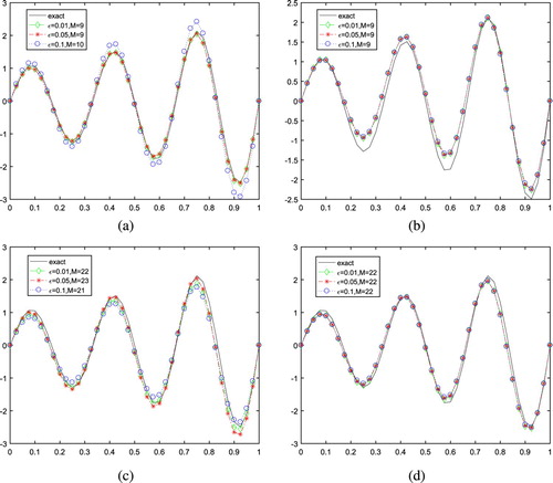
When $\gamma =0.6,$ it is the fractional Landweber regularization method, the numerical results are in very agreement with the exact shape and the iteration steps are few with the noise level $\epsilon =0.01$ and accelerated factor $\mu =6$. When $\gamma =1,$ it is the Landweber regularization method, the numerical results are not in agreement with the exact shape and there are many iterative steps with the noise level $\epsilon =0.01$ and accelerated factor $\mu =6$. The fractional Tikhonov regularization method and the Tikhonov regularization method are also valid for this problem, you can see Figure 2.

Figure 2. Exact solution and numerical solution $f(x)$ of Example 6.1 for various value of γ with fixed $\mu =6$, $\epsilon =0.01$. (a) Numerical solution for $\alpha =1.3$, $\beta =1.2$. (b) Numerical solution for $\alpha =1.7$, $\beta =1.2$. (c) Numerical solution for $\alpha =1.3$, $\beta =1.6$. (d) Numerical solution for $\alpha =1.7$, $\beta =1.6$.

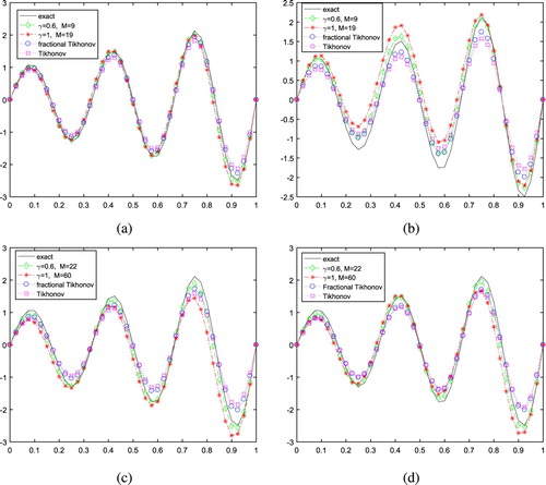
Example 6.2

Let $d=1,\mu =6,\gamma =0.6$. For this case, we know that ${\lambda }_n=n^2{\pi }^2$ and ${\phi }_n=\sqrt{2}\sin (n\pi x)$. Take $a(x)=x^{1+\alpha +\beta }(1-x{)}^{1+\alpha +\beta },b(x)=x^{2+\alpha +\beta }(1-x{)}^{2+\alpha +\beta },f(x)=3\sin (5\pi x)+x^{1+\alpha +\beta }(1-x{)}^{\alpha +\beta },$ the final data $g(x)$ is obtain by finite difference.

The numerical results for Example 6.2 with various noise levels $\epsilon =0.01,0.05,0.10$ in the case of $\alpha =1.3,1.7,\beta =1.2,1.6$. It can be seen from Figure 3 that different α, β and ε have different fitting effects.

Figure 3. Exact solution and numerical solution $f(x)$ for Example 6.2 with different $\alpha ,\beta$ and ε. (a) Numerical solution for $\alpha =1.3$, $\beta =1.2$. (b) Numerical solution for $\alpha =1.7$, $\beta =1.2$. (c) Numerical solution for $\alpha =1.3$, $\beta =1.6$. (d) Numerical solution for $\alpha =1.7$, $\beta =1.6$.

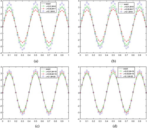
Example 6.3

Let $d=2,\mu =6,\gamma =0.6$. For this case, we know that ${\lambda }_{mn}=(m^2+n^2){\pi }^2$ and ${\phi }_{mn}=2\sin (m\pi x)\sin (n\pi y)$. Take $a(x,y)=x^{1+\alpha }(1-x{)}^{1+\alpha }{y}^{1+\alpha }(1-y{)}^{1+\alpha },b(x,y)=x^{1+\alpha }(1-x{)}^{1+\alpha }{y}^{1+\alpha }(1-y{)}^{1+\alpha },f(x,y)=\sin (3\pi x)\sin (3\pi y)+x^{1+\alpha }(1-x{)}^{1+\alpha }{y}^{1+\alpha }(1-y{)}^{1+\alpha },$ the final data $g(x,y,T)$ is obtain by finite difference.

Figure 4 present the exact solution and the regularized solutions for Example 6.3 with a noise level $\epsilon =0.01$ in the case of $\alpha =1.3,1.7$, $\beta =1.2,1.6$. Figure 5 present the absolute error with $\alpha =1.3,1.7$, $\beta =1.2,1.6$. It can be observed that the proposed method gives the accurate numerical reconstructions.

Figure 4. Exact solution and numerical solution $f(x)$ for Example 6.3 with different α and β. (a) Numerical solution for $\alpha =1.3$, $\beta =1.2$. (b) Numerical solution for $\alpha =1.7$, $\beta =1.2$. (c) Numerical solution for $\alpha =1.3$, $\beta =1.6$. (d) Numerical solution for $\alpha =1.7$, $\beta =1.6$. (e) Exact solution.

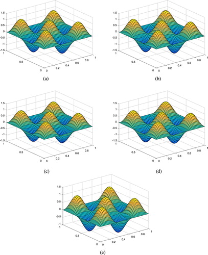
Figure 5. The absolute error for Example 6.3 with different α and β. (a) $\alpha =1.3$, $\beta =1.2$. (b) $\alpha =1.7$, $\beta =1.2$. (c) $\alpha =1.3$, $\beta =1.6$. (d) $\alpha =1.7$, $\beta =1.6$.

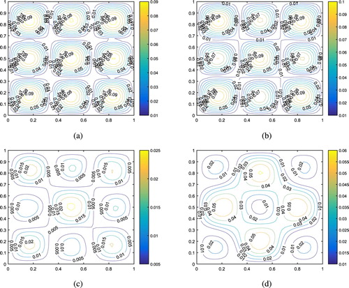
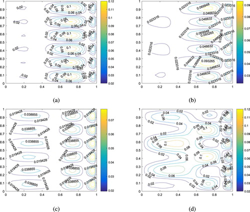
Example 6.4

Let d = 2, $\mu =6$, $\gamma =0.6$. For this case, we know that ${\lambda }_{mn}=(m^2+n^2){\pi }^2$ and ${\phi }_{mn}=2\sin (m\pi x)\sin (n\pi y)$. Take $a(x,y)=x^{1+\alpha }(1-x{)}^{1+\alpha }{y}^{1+\alpha }(1-y{)}^{1+\alpha },b(x,y)=x^{1+\alpha }(1-x{)}^{1+\alpha }{y}^{1+\alpha }(1-y{)}^{1+\alpha },f(x,y)=5\sin (6\pi x)e^{3y}{y}^2(1-y{)}^2,$ the final data $g(x,y,T)$ is obtain by finite difference.

Figure 6 present the exact solution and the regularized solutions for Example 6.4 with a noise level $\epsilon =0.01$ in the case of $\alpha =1.3,1.7$, $\beta =1.2,1.6$. Figure 7 present the absolute error with $\alpha =1.3,1.7$, $\beta =1.2,1.6$. It can be observed that the proposed method gives the accurate numerical reconstructions.

Figure 6. Exact solution and numerical solution $f(x)$ for Example 6.4 with different α and β. (a) Numerical solution for $\alpha =1.3$, $\beta =1.2$. (b) Numerical solution for $\alpha =1.7$, $\beta =1.2$. (c) Numerical solution for $\alpha =1.3$, $\beta =1.6$. (d) Numerical solution for $\alpha =1.7$, $\beta =1.6$. (e) Exact solution.

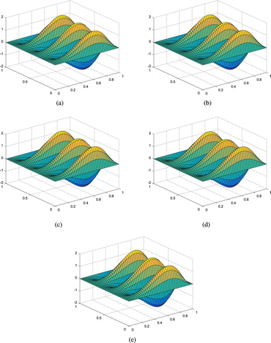
Figure 7. The absolute error for Example 6.4 with different α and β. (a) $\alpha =1.3$, $\beta =1.2$. (b) $\alpha =1.7$, $\beta =1.2$. (c) $\alpha =1.3$, $\beta =1.6$. (d) $\alpha =1.7$, $\beta =1.6$.

In Table 1, we display the relative error E and iteration steps for Example 6.1 with various value of μ in which we fixed $\alpha =1.1$, $\beta =1.6$, $\epsilon =0.01$. From Table 1, we can draw some conclusions. When accelerated factor $\mu \in (0,20),$ as accelerated factor increases, the fractional Landweber regularization method converges faster (iterative steps decrease). When accelerated factor $\mu \in (20,75),$ the number of iteration steps have a smaller change with the various μ. When accelerated factor $\mu \in (75,\mathrm{\infty }),$ after iterate one step, the fractional Landweber regularization method will not converge. Through experiments, about other Examples 6.2–6.4, we also reached the same conclusion.

Table 1. The relative errors E and iteration steps of Example 6.1 for various value of μ with fixed $\alpha =1.1$, $\beta =1.6$, $\gamma =0.6$, $\epsilon =0.01$.

$\epsilon \setminus \mu$	0.01	0.1	1	10	20	70	75
0.01	0.039(249)	0.039(104)	0.037(44)	0.033(18)	0.031(14)	0.032(9)	0.231(1)

In Tables 2–5, we display the relative error E and iteration steps for Examples 6.1–6.4 with various value of β and γ in which we fixed $\alpha ,\mu =6,\epsilon =0.01$. From Tables 2–5, we can draw some conclusions. The numerical results are good and the iteration steps are few with $\gamma =0.6$. The numerical results are not good and there are many iterative steps with $\gamma =1$. When $\gamma =0.6$ or $\gamma =1,$ the number of iteration steps increase with the increase of β, but different α and β have different relative errors.

Table 2. The relative errors E and iteration steps of Example 6.1 for various value of β and γ with fixed $\alpha =1.1$, $\mu =6$, $\epsilon =0.01$.

β	1.1	1.3	1.5	1.7	1.9
$\gamma =0.6$	0.051(7)	0.060(11)	0.083(17)	0.061(27)	0.064(42)
$\gamma =1$	0.0105(15)	0.093(27)	0.097(44)	0.098(79)	0.10(157)

Table 3. The relative errors E and iteration steps of Example 6.2 for various value of β and γ with fixed $\alpha =1.3$, $\mu =6$, $\epsilon =0.01$.

β	1.1	1.3	1.5	1.7	1.9
$\gamma =0.6$	0.094(6)	0.052(10)	0.037(15)	0.045(22)	0.032(34)
$\gamma =1$	0.147(11)	0.0768(21)	0.0798(36)	0.0935(62)	0.1184(107)

Table 4. The relative errors E and iteration steps of Example 6.3 for various value of β and γ with fixed $\alpha =1.7$, $\mu =6$, $\epsilon =0.01$.

β	1.1	1.3	1.5	1.7	1.9
$\gamma =0.6$	0.086(6)	0.019(9)	0.045(12)	0.066(18)	0.083(27)
$\gamma =1$	0.083(11)	0.041(19)	0.056(26)	0.196(47)	0.287(76)

Table 5. The relative errors E and iteration steps of Example 6.4 for various value of β and γ with fixed $\alpha =1.5$, $\mu =6$, $\epsilon =0.01$.

β	1.1	1.3	1.5	1.7	1.9
$\gamma =0.6$	0.086(7)	0.051(12)	0.054(18)	0.048(29)	0.048(45)
$\gamma =1$	0.088(14)	0.065(27)	0.086(49)	0.113(87)	0.10(157)

In Tables 6–9, we display the relative error E and iteration steps for Examples 6.1–6.4 with various value of α and γ in which we fixed $\beta ,\mu =6,\epsilon =0.01$. From Tables 6–9, we can draw some conclusions. The numerical results are good and the iteration steps are few with $\gamma =0.6$. The numerical results are not good and there are many iterative steps with $\gamma =1$. When $\gamma =0.6$ or $\gamma =1,$ the number of iteration steps have a smaller change with the increase of α, but different α and β have different relative errors.

Table 6. The relative errors E and iteration steps of Example 6.1 for various value of α and γ with fixed $\beta =1.9$, $\mu =6$, $\epsilon =0.01$.

α	1.1	1.3	1.5	1.7	1.9
$\gamma =0.6$	0.064(43)	0.063(43)	0.045(45)	0.0448(45)	0.064(43)
$\gamma =1$	0.96(142)	0.082(143)	0.0804(143)	0.0684(144)	0.1013(172)

Table 7. The relative errors E and iteration steps of Example 6.2 for various value of α and γ with fixed $\beta =1.7$, $\mu =6$, $\epsilon =0.01$.

α	1.1	1.3	1.5	1.7
$\gamma =0.6$	0.0534(22)	0.0437(22)	0.0328(22)	0.0504(23)
$\gamma =1$	0.1341(62)	0.0935(62)	0.0755(64)	0.0109(64)

Table 8. The relative errors E and iteration steps of Example 6.3 for various value of α and γ with fixed $\beta =1.5$, $\mu =6$, $\epsilon =0.01$.

α	1.1	1.3	1.5	1.7	1.9
$\gamma =0.6$	0.024(12)	0.018(12)	0.0177(12)	0.045(12)	0.031(13)
$\gamma =1$	0.042(28)	0.093(29)	0.096(29)	0.084(28)	0.115(29)

Table 9. The relative errors E and iteration steps of Example 6.4 for various value of α and γ with fixed $\beta =1.3$, $\mu =6$, $\epsilon =0.01$.

α	1.1	1.3	1.5	1.7	1.9
$\gamma =0.6$	0.050(12)	0.053(12)	0.055(12)	0.053(11)	0.060(14)
$\gamma =1$	0.063(26)	0.1156(25)	0.1140(25)	0.0946(26)	0.1135(31)

7. Conclusion

In this paper, we consider the recovering space-dependent source problem for the time-space fractional diffusion wave equation defined in a bounded domain. The inverse problem has been transformed into an integral equation. The conditional stability for the inverse problem is discussed. We use the fractional Landweber regularization method for overcoming the ill-posedness. The convergence rates are obtained for the inverse problem under an a priori and an a posteriori regularization parameter choice rulers, respectively. The numerical experiments for four examples show that our proposed method is effective.

Disclosure statement

No potential conflict of interest was reported by the author(s).

Additional information

Funding

This paper was supported by the National Natural Science Foundation (NSF) of China [grant number 11471150].

References

- Chen W, Holm S. Physical interpretation of fractional diffusion wave equation via Lossy media obeying frequency power law; 2003. Available from: https://arxiv.org/abs/math-ph/0303040.
- Sakamoto K, Yamamoto M. Initial value/boundary value problems for fractional diffusion-wave equations and applications to some inverse problems. J Math Anal Appl. 2011;382:426–447. doi: 10.1016/j.jmaa.2011.04.058
- Du R, Cao WR, Sun ZZ. A compact difference scheme for the fractional diffusion-wave equation. Appl Math Model. 2010;34:2998–3007. doi: 10.1016/j.apm.2010.01.008
- Agrawal OP. Solution for a fractional diffusion wave equation defined in a bounded domain. Nonlinear Dyn. 2002;29:145–155. doi: 10.1023/A:1016539022492
- Jiang H, Liu F, Turner I, et al. Analytical solutions for the multi-term time fractional diffusion wave/diffusion equations in a finite domain. Comput Math Appl. 2012;64:3377–3388. doi: 10.1016/j.camwa.2012.02.042
- Chen A, Li C. Numerical solution of fractional diffusion wave equation. Numer Funct Anal Optim. 2016;37:19–39. doi: 10.1080/01630563.2015.1078815
- Dai H, Wei L, Zhang X. Numerical algorithm based on an implicit fully discrete local discontinuous Galerkin method for the fractional diffusion wave equation. Numer Algorithms. 2014;67:845–862. doi: 10.1007/s11075-014-9827-y
- Zhou Y, He JW, Ahmad B, et al. Existence and regularity results of a backward problem for fractional diffusion equations. Math Methods Appl Sci. 2019;42(18):6775–6790. doi: 10.1002/mma.5781
- Tuan NH, Huynh LN, Ngoc TB, et al. On a backward problem for nonlinear fractional diffusion equations. Appl Math Lett. 2019;92:76–84. doi: 10.1016/j.aml.2018.11.015
- Wei T, Zhang Y. The backward problem for a time-fractional diffusion-wave equation in a bounded domain. Comput Math Appl. 2018;75:3632–3648. doi: 10.1016/j.camwa.2018.02.022
- Huynh LN, Zhou Y, Oregan D, et al. Fractional Landweber method for an initial inverse problem for time-fractional wave equation. Appl Anal. 2019; Available From: https://doi.org/10.1080/00036811.2019.1622682.
- Yang F, Zhang Y, Li XX. Landweber iterative method for identifying the initial value problem of the time-space fractional diffusion wave equation. Numer Algorithms. 2020;83:1509–1530. doi: 10.1007/s11075-019-00734-6
- Jiang SZ, Liao KF, Wei T. Inversion of the initial value for a time-fractional diffusion wave equation by boundary data. Comput Methods Appl Math. 2020;20:109–120. doi: 10.1515/cmam-2018-0194
- Xian J, Wei T. Determination of the initial data in a time fractional diffusion wave problem by a final time data. Comput Math Appl. 2019;78(8):2525–2540. doi: 10.1016/j.camwa.2019.03.056
- Liao KF, Li YS, Wei T. The identification of the time dependent source term in time fractional diffusion wave equations. East Asian J Appl Math. 2019;9(2):330–354. doi: 10.4208/eajam.250518.170119
- Gong X, Wei T. Reconstruction of a time-dependent source term in a time fractional diffusion equation. Inverse Probl Sci Eng. 2019;27:1577–1594. doi: 10.1080/17415977.2018.1539481
- Siskova K, Slodicka M. Recognition of a time-dependent source in a time fractional diffusion wave equation. Appl Numer Math. 2017;121:1–17. doi: 10.1016/j.apnum.2017.06.005
- Lopushansky A, Lopushanska H. Inverse source Cauchy problem for a time fractional diffusion wave equation with distributions. Electron J Differ Equ. 2017;2017:1–14. doi: 10.1186/s13662-016-1057-2
- Kian Y, Oksanen L, Soccorsi E, et al. Global uniqueness in an inverse problem for time fractional diffusion equations. J Differ Equ. 2018;264(2):1146–1170. doi: 10.1016/j.jde.2017.09.032
- Yang F, Liu X, Li XX, et al. Landweber iterative regularization method for identifying the unknown source of the time fractional diffusion equation. Adv Differ Equ. 2017;2017:149. doi: 10.1186/s13662-017-1205-3
- Yan XB, Wei T. Determine a space-dependent source term in a time fractional diffusion wave equation. Acta Appl Math. 2020;165:163–181. doi: 10.1007/s10440-019-00248-2
- Klann E, Ramlau R. Regularization by fractional filter methods and data smoothing. Inverse Prob. 2008;24(2):045005. doi: 10.1088/0266-5611/24/2/025018
- Han YZ, Xiong XT, Xue XM. A fractional Landweber method for solving backward time fractional diffusion problem. Comput Math Appl. 2019;78:81–91. doi: 10.1016/j.camwa.2019.02.017
- Tatar S, Tnaztepe R, Ulusoy S. Determination of an unknown source term in a space-time fractional diffusion equation. Fract Calc Appl Anal. 2015;6(1):83–90.
- Tatar S, Tnaztepe R, Ulusoy S. Simultaneous inversion for the exponents of the fractional time and space derivative in the space-time fractional diffusion equation. Appl Anal. 2016;95(1):1–23. doi: 10.1080/00036811.2014.984291
- Tatar S, Ulusoy S. An inverse source problem for a one-dimensional space-time fractional diffusion equation. Appl Anal. 2015;94(11):2233–2244. doi: 10.1080/00036811.2014.979808
- Podlubny I. Fractional differential equations. San Diego (CA): Academic Press; 1999.
- Kilbas A, Srivastava H, Trujillo J. Theory and applications of fractional differential equations. Vol. 204. Amsterdam: Elsevier; 2006. p. 2453–2461.
- Engl HW, Hanke M, Neubauer A. Regularization of inverse problems, mathematics and its applications. Dordrecht: Kluwer Academic Publishers Group; 1996.
- Li YS, Wei T. An inverse time dependent source problem for a time space fractional diffusion equation. Appl Math Comput. 2018;336:257–271.
- Zhang Y, Sun Z. Alternating direction implicit schemes for the two-dimensional fractional sub-diffusion equation. J Comput Phys. 2011;230(24):8713–8728. doi: 10.1016/j.jcp.2011.08.020